Optimal Configurations in Coverage Control with Polynomial Costs

Abstract

We revisit the static coverage control problem for placement of vehicles with simple motion on the real line, under the assumption that the cost is a polynomial function of the locations of the vehicles. The main contribution of this paper is to demonstrate the use of tools from numerical algebraic geometry, in particular, a numerical polynomial homotopy continuation method that guarantees to find all solutions of polynomial equations, in order to characterize the global minima for the coverage control problem. The results are then compared against a classic distributed approach involving the use of Lloyd descent, which is known to converge only to a local minimum under certain technical conditions.

1 Introduction

Vehicle placement to provide optimal coverage has received lot of attention, especially in the past two decades. The goal is to determine where to place vehicles in order to optimize a specified cost that is a function of the locations of the vehicles. This paper addresses the characterization of the global minima for a vehicle placement problem under the assumption that this cost function is polynomial in the locations of the vehicles. It is well known that polynomials can be used as building blocks to describe several realistic functions. Applications of this work are envisioned in border patrol wherein unmanned vehicles are placed to optimally intercept moving targets that cross a region under surveillance (cf. Girard et al. (2004); Szechtman et al. (2008)).

Vehicle placement problems are analogous to geometric location problems, wherein given a set of static points, the goal is to find supply locations that minimize a cost function of the distance from each point to its nearest supply location (cf. Zemel (1985)). For a single vehicle, the expected distance to a point that is randomly generated via a probability density function, is given by the continuous $1$–median function. The $1$–median function is minimized by a point termed as the median (cf. Fekete et al. (2005)). For multiple distinct vehicle locations, the expected distance between a randomly generated point and one of the locations is known as the continuous multi-median function (cf. Drezner and Hamacher (2001)). For more than one location, the multi-median function is non-convex and thus determining locations that minimize the multi-median function is hard in the general case. Cortes et al. (2004) addressed a distributed version of a partition and gradient based procedure, known as the Lloyd algorithm, for deploying multiple robots in a region to optimize a multi-median cost function. Schwager et al. (2009) provided an adaptive control law to enable robots to approximate the density function from sensor measurements. Martínez and Bullo (2006) presented motion coordination algorithms to steer a mobile sensor network to an optimal placement. Kwok and Martínez (2010) presented a coverage algorithm for vehicles in a river environment. Related forms of the cost function have also appeared in disciplines such as vector quantization, signal processing and numerical integration (cf. Gray and Neuhoff (1998); Du et al. (1999)).

In this paper, we consider the static coverage control problem for placement of vehicles with simple motion on the real line. We assume that the cost is a polynomial function of the locations of the vehicles. This structure implies that the set of all candidate optima is finite. The main contribution of this paper is to demonstrate the use of tools from numerical algebraic geometry, in particular, a numerical polynomial homotopy continuation method that guarantees to find all solutions of the polynomial equations (cf. Sommese and Wampler (2005) and Bates et al. (2013)). Such methods have been used in a variety of problems, e.g., computing all finite and infinite equilibria for constructing one-dimensional slow invariant manifolds of dynamical systems (cf.  Al-Khateeb et al. (2009)) and finding all equilibria of the Kuramoto model (cf. Mehta et al. (2015)). Upon computing the finite set of candidate optima, we can evaluate the cost function at these points to obtain the global minimum for the coverage control problem. The results are then compared numerically using two examples with a classic distributed approach involving the use of Lloyd descent, which is known to converge only to a local minimum under certain technical conditions. We observe that in one of the examples, both methods lead to the same global minimizer, while in the second example, the Lloyd descent converges to only a local minimum if initialized from particular configurations.

This paper is organized as follows. The problem is formulated in Section 2. The multiple vehicle scenario is addressed in Section 3. The polynomial homotopy method is reviewed and its application to the coverage problem is presented in Section 4. Numerical simulation results are presented in Section 5.

2 Problem Statement

We consider vehicles modeled with single integrator dynamics having unit speed. A static target is generated at a random position $x\in[A,B]$ on the segment $G:=[A,B]$, via a specified probability density function $\phi:[A,B]\rightarrow{\mathbb{R}}_{\geq 0}$. We assume that the density $\phi$ is bounded, and therefore integrable over a compact domain. The goal is to determine vehicle placements that minimize the expected time for the nearest vehicle to reach a target. We consider the both the single and multiple vehicle cases.

2.1 Single Vehicle Case

We determine a vehicle location $p\in[A,B]$ that minimizes ${C}_{\textup{exp}}:[A,B]\rightarrow{\mathbb{R}}$ given by

$${C}_{\textup{exp}}(p):=\int_{A}^{B}C(p,x)\phi(x)dx,$$ (1)

where $C:[A,B]\times[A,B]\rightarrow{\mathbb{R}}_{\geq 0}$ is an appropriately defined cost of the vehicle position $p$ and the target location $x$. In what follows, we consider costs with the following properties.

(i) Polynomial dependence on $p$: We assume that for any $p\in[A,B]$, the cost function $C$ is polynomial in $p$.

(ii) Homogeneity: We assume that the function $C$ satisfies

$$C(p,x)=\frac{1}{2}f((p-x)^{2}),$$

where $f(\cdot)\geq 0$ is a polynomial and is monotonic with respect to its argument.

2.2 Multiple Vehicles Case

Given $m\geq 2$ vehicles, the goal is to determine a set of vehicle locations $p_{i}$, for every $i\in\{1,\dots,m\}$, that minimizes the expected cost given by

$${C}_{\textup{exp}}(p_{1},\dots,p_{m}):=\int_{A}^{B}\min_{i\in\{1,\dots,m\}}C(p_{i},x)\phi(x)dx,$$ (2)

where $C(p_{i},x)$ satisfies the same properties that are assumed in Section 2.1. The single vehicle case shall then follow as a special case of multiple vehicles.

3 The Case of Multiple Vehicles

Consider the multiple vehicle case from Section 2.2 with assumptions (i) and (ii) from Section 2.1. We will require the concept of dominance regions. For the $i$-th vehicle, the dominance region $\mathcal{V}_{i}$ is defined as

$$\mathcal{V}_{i}:=\{x\in[A,B]\,:\,C(p_{i},x)\leq C(p_{j},x),\forall j\neq i\}.$$

In other words, $\mathcal{V}_{i}$ is the set of all points $x$ for which an assignment of any point in that set to vehicle $i$ provides the least cost over assignment to any other vehicle. The following proposition provides a simple approach to computing the dominance regions.

Proposition 3.1

Under Assumption (ii), the dominance region of the $i$-th vehicle is the Euclidean Voronoi partition corresponding to the $i$-th vehicle, i.e.,

$$\mathcal{V}_{i}=\{x\in[A,B]\,:\,|p_{i}-x|\leq|p_{j}-x|,\forall j\neq i\}.$$

Proof: From the definition of $\mathcal{V}_{i}$, we have

$$C(p_{i},x)\leq C(p_{j},x)\\ \Rightarrow(p_{i}-x)^{2}\leq(p_{j}-x)^{2}\Rightarrow|p_{i}-x|\leq|p_{j}-x|,$$

from the monotonicity in Assumption (ii).   

Without any loss of generality, let the vehicles be placed with their indices in ascending order on $[A,B]$. Then,

$$\mathcal{V}_{i}=\begin{cases}[A,(p_{1}+p_{2})/2],&i=1,\\ [(p_{i-1}+p_{i})/2,(p_{i}+p_{i+1})/2],&i\in\{2,\dots,m-1\},\\ [(p_{m-1}+p_{m})/2,B],&i=m.\end{cases}$$

3.1 Minimizing the Expected Constrained Travel Time

For distinct vehicle locations, (2) can be written as

$${C}_{\textup{exp}}(p_{1},\dots,p_{m})=\sum_{i=1}^{m}\int_{\mathcal{V}_{i}}C(p_{i},x)\phi(x)dx,$$ (3)

where $\mathcal{V}_{i}$ is the dominance region of the $i$-th vehicle. The gradient of ${C}_{\textup{exp}}$ is computed using the following formula, which allows each vehicle to compute the gradient of ${C}_{\textup{exp}}$ by integrating the gradient of $C$ over $\mathcal{V}_{i}$.

Proposition 3.2 (Gradient computation)

For all vehicle configurations such that no two vehicles are at coincident locations, the gradient of the expected time with respect to vehicle location $p_{i}$ is

$$\frac{\partial{C}_{\textup{exp}}}{\partial p_{i}}=\int_{\mathcal{V}_{i}}\frac{\partial C}{\partial p_{i}}(p_{i},x)\phi(x)dx.$$

Proof: Akin to similar results in Bullo et al. (2009), the following involves writing the gradient of ${C}_{\textup{exp}}$ as a sum of two contributing terms. The first is the final expression, while the second is a number of terms which cancel out due to continuity of $C$ at the boundaries of dominance regions.

Let $p_{j}$ be termed as a neighbor of $p_{i}$, i.e., $j\in$ neigh$(i)$, if $\mathcal{V}_{i}\cap\mathcal{V}_{j}$ is non-empty. Then,

$$\frac{\partial{C}_{\textup{exp}}}{\partial p_{i}}=\frac{\partial}{\partial p_{i}}\int_{\mathcal{V}_{i}}C(p_{i},x)\phi(x)dx\\ +\sum_{j\text{ neigh }(i)}\frac{\partial}{\partial p_{i}}\int_{\mathcal{V}_{j}}C(p_{j},x)\phi(x)dx,$$ (4)

Now, from the expression of $\mathcal{V}_{i}$, there arise three cases:

1. $i\in\{2,\dots,m-1\}$: In this case, all boundary points $(p_{i-1}+p_{i})/2$ and $(p_{i}+p_{i+1})/2$ are differentiable with respect to $p_{i}$. Therefore, by Leibnitz’s Rule,

$$\frac{\partial}{\partial p_{i}}\int_{\mathcal{V}_{i}}C(p_{i},x)\phi(x)dx-\int_{\mathcal{V}_{i}}\frac{\partial C}{\partial p_{i}}\phi(x)dx$$

$$=\frac{1}{2}\left(C\left(p_{i},\frac{p_{i}+p_{i+1}}{2}\right)-C\left(p_{i},\frac{p_{i}+p_{i-1}}{2}\right)\right)$$

$$=\frac{1}{2}\left(f\left(\left(\frac{p_{i+1}-p_{i}}{2}\right)^{2}\right)-f\left(\left(\frac{p_{i}-p_{i-1}}{2}\right)^{2}\right)\right),$$

where the second step follows from Assumption (ii).

Using the same steps by applying the Leibnitz rule, we conclude that

$$\frac{\partial}{\partial p_{i}}\int_{\mathcal{V}_{i-1}}C(p_{i-1},x)\phi(x)dx =\frac{1}{2}f\left(\left(\frac{p_{i}-p_{i-1}}{2}\right)^{2}\right)$$

$$\frac{\partial}{\partial p_{i}}\int_{\mathcal{V}_{i+1}}C(p_{i+1},x)\phi(x)dx =-\frac{1}{2}f\left(\left(\frac{p_{i+1}-p_{i}}{2}\right)^{2}\right).$$

Therefore, combining these three expressions into (4), we conclude that for this case,

$$\frac{\partial{C}_{\textup{exp}}}{\partial p_{i}}=\int_{\mathcal{V}_{i}}\frac{\partial C}{\partial p_{i}}(p_{i},x)\phi(x)dx.$$

2. $i=1$: In this case, the lower limit of the integral below is $A$ and is a constant. Therefore, applying the Leibnitz rule, we obtain

$$\frac{\partial}{\partial p_{1}}\int_{\mathcal{V}_{1}}C(p_{1},x)\phi(x)dx=\int_{\mathcal{V}_{1}}\frac{\partial C}{\partial p_{1}}\phi(x)dx+\frac{1}{2}f\left(\left(\frac{p_{2}-p_{1}}{2}\right)^{2}\right).$$

Applying the Leibnitz rule for the corresponding term involving the neighbor $p_{2}$, we obtain

$$\frac{\partial}{\partial p_{1}}\int_{\mathcal{V}_{2}}C(p_{2},x)\phi(x)dx=-\frac{1}{2}f\left(\left(\frac{p_{2}-p_{1}}{2}\right)^{2}\right)$$

Therefore, combining these two expressions into (4), we conclude that for this case,

$$\frac{\partial{C}_{\textup{exp}}}{\partial p_{1}}=\int_{\mathcal{V}_{1}}\frac{\partial C}{\partial p_{1}}(p_{1},x)\phi(x)dx.$$

The third case of $i=m$ is very similar to the case of $i=1$ and the conclusion analogous to that of $i=1$ can be verified. Therefore, the claim is verified for each case.   

Remark 3.3 (Infinite interval)

The formulation can easily be extended to the case when the domain for the vehicles is unbounded, i.e., ${\mathbb{R}}$. In that case, we will require an extra assumption on the weight function $\phi$ which would be that as $x\to\pm\infty$, $\phi(x)\to 0^{+}$ while $C(x)$ remains bounded.

The expressions for the gradient can then be used within the Lloyd descent algorithm (see for example Bullo et al. (2009)) to derive a control scheme for each vehicle to move, beginning with an initial arbitrary, non-degenerate configuration using the following steps iteratively: while a given number of iterations are not reached,

1. Each vehicle computes its Voronoi partition $\mathcal{V}_{i}$,

2. Each vehicle computes the gradient of the cost function using Proposition 3.2,

3. Each vehicle computes its step size using backtracking line search, and

4. Each vehicle uses gradient descent to compute its new position.

In the following subsection, we will address computing the global optima by posing the set of equations that need to be solved in order to compute the candidate points.

3.2 Optimal Placement

The optimal vehicle placement problem is cast as

$$\min_{\{p_{1},\dots,p_{n}\}\in[A,B]^{m}}{C}_{\textup{exp}}(p_{1},\dots,p_{m})$$

$$\text{subject to }p_{i}\in[A,B],\forall i\in\{1,\dots,m\}.$$

Without loss of generality, we assume that the vehicles are located such that $p_{i-1}<p_{i}<p_{i+1}$. Then, the candidate global minima are:

1. $p_{1}^{*}=A$ and the set of all points $p_{i}^{*},i=2,\dots,m$, for which

   $$\frac{\partial{C}_{\textup{exp}}}{\partial p_{i}}(p_{1}^{*},\dots,p_{m}^{*})=0,$$

2. $p_{m}^{*}=B$ and the set of all points $p_{i}^{*},i=1,\dots,m-1$, for which

   $$\frac{\partial{C}_{\textup{exp}}}{\partial p_{i}}(p_{1}^{*},\dots,p_{m}^{*})=0,$$

   or,

3. the set of all points $p_{i}^{*},i=1,\dots,m$, for which

   $$\frac{\partial{C}_{\textup{exp}}}{\partial p_{i}}(p_{1}^{*},\dots,p_{m}^{*})=0,$$

along with the additional condition on the Hessian

$$\frac{\partial^{2}{C}_{\textup{exp}}}{\partial\mathbf{p}^{2}}(p_{1}^{*},\dots,p_{m}^{*})\succ 0,$$

where $\mathbf{p}:=[p_{1},\dots,p_{m}]$. Proposition 3.2 provides a simple expression for the computation of the partial derivatives of ${C}_{\textup{exp}}$. The set of all candidate can be characterized by

$$\int_{A}^{\frac{p_{1}+p_{2}}{2}}f^{\prime}\left((p_{1}-x)^{2}\right)(p_{1}-x)\phi(x)dx =0,$$

$$\int_{\frac{p_{m-1}+p_{m}}{2}}^{B}f^{\prime}\left((p_{m}-x)^{2}\right)(p_{m}-x)\phi(x)dx =0,$$

and, for $2\leq i\leq m-1$,

$$\int_{\frac{p_{i-1}+p_{i}}{2}}^{\frac{p_{i}+p_{i+1}}{2}}f^{\prime}\left((p_{i}-x)^{2}\right)(p_{i}-x)\phi(x)dx =0$$

Now let us call the integral

$$F(p,b,a):=\int_{a}^{b}f^{\prime}\left((p-x)^{2}\right)(p-x)\phi(x)dx$$

Notice that under Assumption (ii), $F(p,b,a)$ is also a polynomial in $p$. Then, the candidates for global minima are given by the set of polynomial equations:

$$F\left(p_{1},\frac{p_{1}+p_{2}}{2},A\right) =0$$

$$F\left(p_{i},\frac{p_{i+1}+p_{i}}{2},\frac{p_{i}+p_{i-1}}{2}\right) =0\quad\forall i\in\{2,\dots,m-1\},$$

$$F\left(p_{m},B,\frac{p_{m-1}+p_{m}}{2}\right) =0,$$ (5)

with the additional possibility that $p_{1}=A$ or $p_{m}=B$. In the next section, we will review techniques from numerical algebraic geometry to explore the full spectrum of solutions for (3.2) and therefore compute the global optimum.

4 Polynomial system of equations through Algebraic Geometry

Typically, performing an exhaustive search of solutions of systems of nonlinear equations such as (3.2) is a prohobitively difficult task. However, in this paper, by restricting ourselves to polynomial conditions, this becomes feasible. Furthermore, though in the original formulation only requires computing real solutions of the system, we expand our search space to complex space, i.e., instead of $\textbf{p}\in\mathbb{R}^{n}$ we take $\textbf{p}\in\mathbb{C}^{n}$. The purpose of the complexification of the variables is to enable us to use some of the powerful mathematical and computational tools from algebraic geometry, i.e., in mathematical terms, $\mathbb{C}^{n}$ is the algebraic closure of $\mathbb{R}^{n}$. In particular, we utilize the numerical algebraic geometric computational technique called the numerical polynomial homotopy continuation (NPHC) method which guarantees (in the probability 1 sense) to compute all complex isolated solutions of a well-constrained system of multivariate polynomial equations. More details are provided in the books by Sommese and Wampler (2005) and Bates et al. (2013).

For a well-constrained system of polynomial equations (also called a square system which has the same number of equations and variables) $\textbf{F}(\textbf{p})=\textbf{0}$, classical NPHC method uses a single homotopy that starts with an upper bound on the number of isolated complex solutions. One standard upper bound is the classical Bézout bound (CBB) which is simply the product of the degrees of the polynomials, namely $\prod_{i=1}^{n}d_{i}$ where $d_{i}=\deg{\bf F}_{i}$ and $n$ is the number of polynomials in ${\bf F}$. Although the CBB is trivial to compute, it does not take structure (such as sparsity or sparsity) of the system into account. There are tighter bounds such as the multihomogeneous Bézout bound and the polyhedral, also called the Bernshtein-Kushnirenko-Khovanskii (BKK), bound can exploit some structure in the system to provide a tighter upper bound using possibly significant additional computations.

Each such upper bound yields a corresponding system $\textbf{G}(\textbf{p})=\textbf{0}$, called a start system, where the bound is sharp. For example, the CBB yields

$$\textbf{G}(\textbf{p})=[p_{1}^{d_{1}}-1,\dots,p_{n}^{d_{n}}-1]={\bf 0}$$

which clearly has $\prod_{i=1}^{n}d_{i}$ isolated solutions. For other upper bounds, the procedure of constructing a start system may be more involved. Once a start system is constructed, a homotopy between $\textbf{F}(\textbf{p})$ and $\textbf{G}(\textbf{p})$ is constructed as

$$\textbf{H}(\textbf{p},t)=(1-t)\textbf{F}(\textbf{p})+e^{\theta\sqrt{-1}}\,t\,\textbf{G}(\textbf{p})=\textbf{0}$$

where $\theta\in[0,2\pi)$. One tracks the solution path defined by ${\bf H}={\bf 0}$ from a known solution of ${\bf G}={\bf 0}$ at $t=1$ to $t=0$. For all but finitely many $\theta\in[0,2\pi)$, all solution paths are smooth for $t\in(0,1]$ and the set of isolated solutions of ${\bf F}={\bf 0}$ is contained in the set of limit points of the paths that converge at $t\rightarrow 0^{+}$. Since each path can be tracked independent of each other, the NPHC method is embarrassingly parallelizeable.

To exploit some of the structure in the system (3.2), we first factor each polynomial ${\bf F}_{i}$, say ${\bf F}_{i}=q_{i1}^{r_{i1}}\cdots q_{ik_{i}}^{r_{ik_{i}}}$ where $q_{ij}$ are polynomials and $r_{ij}$ are positive integers. Thus, we can replace each ${\bf F}_{i}$ with a square-free factorization $q_{i1}\cdots q_{ik_{i}}$ to remove trivial singularities caused by $r_{ij}>1$ thereby improving the numerical conditioning of the homotopy paths. Thus, the solutions of ${\bf F}={\bf 0}$ is equal to the union of the solutions of

$${\bf Q}_{j_{1},\dots,j_{n}}=[q_{1j_{1}},\dots,q_{nj_{n}}]={\bf 0}$$

where $1\leq j_{i}\leq k_{i}$ for $i=1,\dots,n$. There are several benefits from such an approach. First, we again improve numerical conditioning of the homotopy paths by solving lower degree systems and with the removal of trivial singularities that arise from solutions that simultaneously solve two or more such systems. Second, this produces additional parallelization opportunity, e.g., by solving each subsystem independently. Rather than having a completely independent solving, we could utilize ideas of regeneration developed by Hauenstein et al. (2011) based on bootstrapping from solving subsystems. To highlight the potential, suppose that one has found that the subsystem ${\bf Q}_{j_{1},\dots,j_{s}}=[q_{1j_{1}},\dots,q_{sj_{s}}]={\bf 0}$ has no solutions, then one immediately knows that ${\bf Q}_{j_{1},\dots,j_{s},j_{s+1},\dots,j_{n}}={\bf 0}$ has no solutions for every $1\leq j_{i}\leq k_{i}$ for $i=s+1,\dots,n$.

For the regeneration approach, fix indices $j_{1},\dots,j_{n}$ such that $1\leq j_{i}\leq k_{i}$ and we aim to solve ${\bf Q}_{j_{1},\dots,j_{n}}={\bf 0}$. Let $\ell_{iu}$ be general linear polynomials for $i=1,\dots,n$ and $u=1,\dots,D_{i}$ where $D_{i}=\deg q_{ij_{i}}$. Consider the polynomial systems

$${\bf G}^{s}_{u_{s+1},\dots,u_{n}}=[q_{1j_{1}},\dots,q_{sj_{s}},\ell_{s+1,u_{s+1}},\dots,\ell_{nu_{n}}].$$

Using linear algebra, we solve ${\bf G}^{0}_{1,\dots,1}={\bf 0}$. Regeneration using a two-stage approach to use the solutions, say $S_{1}$, of ${\bf G}^{s}_{1,\dots,1}={\bf 0}$ to compute the solutions of ${\bf G}^{s+1}_{1,\dots,1}={\bf 0}$ as follows. The first stage, for each $u=2,\dots,D_{s+1}$, uses the homotopy

$$(1-t){\bf G}^{s}_{u,1,\dots,1}+t{\bf G}^{s}_{1,\dots,1}={\bf 0}$$

with start points $S_{1}$ at $t=1$ to compute the solutions $S_{u}$ of ${\bf G}^{s}_{u,1,\dots,1}={\bf 0}$ at $t=0$. By genericity, every path in this homotopy is smooth for $t\in[0,1]$ so that $\#S_{1}=\#S_{u}$. Let $S=\cup_{i=1}^{D_{s+1}}S_{i}$ which are the solutions of

$${\bf K}^{s}_{1,\dots,1}=\left[q_{1j_{1}},\dots,q_{sj_{s}},\prod_{\alpha=1}^{D_{s+1}}\ell_{s+1,\alpha},\ell_{s+2,1},\dots,\ell_{n1}\right]={\bf 0}.$$

Then, the second stage uses the homotopy

$$(1-t){\bf G}^{s+1}_{1,\dots,1}+t{\bf K}^{s}_{1,\dots,1}={\bf 0}$$

with start points $S$ at $t=1$ to compute the solutions of ${\bf G}^{s+1}_{1,\dots,1}={\bf 0}$ as desired. Iterating this process produces the solutions to ${\bf Q}_{j_{1},\dots,j_{n}}={\bf 0}$.

A regeneration-based approach can be advantageous over using a single homotopy when the subsystems have far fewer solutions than the selected upper bound would predict. When the upper bound is not sharp, this causes paths to diverge to infinity resulting in wasted extra computation. This is reduced in regeneration by performing a sequence of homotopies. Likewise, if the upper bound is sharp, then regeneration is not advantageous due to the extra tracking through this sequence. Nonetheless, we can produce all isolated complex solutions using either the classic single homotopy or regeneration which allows us to always compute the global optimum.

5 Simulations

In this section, we numerically evaluate the proposed method and compare it with the classic Lloyd descent algorithm for two choices of the density functions $\phi$. The first scenario is selected in such a way that, for almost all initial configurations, the Lloyd algorithm tends to the global optimum. The second scenario is one in which, from some special initial conditions, the Lloyd algorithm tends to only a particular local optimum.

For the first scenario, we take the interval $[A,B]$ to be $[0,W]$ for $W>0$, $C(p,x)=f\left((p-x)^{2}\right)=(p-x)^{2}$, and the weight function $\phi(x):=x(W-x)$. Then, we have

$$6F(p,b,a)=12\int_{a}^{b}(p-x)x(W-x)dx=\\ \Big{(}b^{2}(6pW-4pb-4Wb+3b^{2})-a^{2}(6pW-4pa-4Wa+3a^{2})\Big{)}.$$

Substituting into the system of equations (3.2), we obtain

$$\Big{(}\frac{p_{1}+p_{2}}{2}\Big{)}^{2}\Big{(}6p_{1}W-4p_{1}\Big{(}\frac{p_{1}+p_{2}}{2}\Big{)}-4W\Big{(}\frac{p_{1}+p_{2}}{2}\Big{)}+3\Big{(}\frac{p_{1}+p_{2}}{2}\Big{)}^{2}\Big{)}=0,$$

$$\Big{(}\frac{p_{3}+p_{2}}{2}\Big{)}^{2}\Big{(}6p_{2}W-4p_{2}\Big{(}\frac{p_{3}+p_{2}}{2}\Big{)}-4W\Big{(}\frac{p_{3}+p_{2}}{2}\Big{)}+3\Big{(}\frac{p_{3}+p_{2}}{2}\Big{)}^{2}\Big{)}$$

$$=\Big{(}\frac{p_{2}+p_{1}}{2}\Big{)}^{2}\Big{(}6p_{2}W-4p_{2}\Big{(}\frac{p_{2}+p_{1}}{2}\Big{)}-4W\Big{(}\frac{p_{2}+p_{1}}{2}\Big{)}+3\Big{(}\frac{p_{2}+p_{1}}{2}\Big{)}^{2}\Big{)},$$

$$W^{2}\Big{(}6p_{3}W-4p_{3}W-4W^{2}+3W^{2}\Big{)}$$

$$=\Big{(}\frac{p_{2}+p_{3}}{2}\Big{)}^{2}\Big{(}6p_{3}W-4p_{3}\Big{(}\frac{p_{2}+p_{3}}{2}\Big{)}-4W\Big{(}\frac{p_{2}+p_{3}}{2}\Big{)}+3\Big{(}\frac{p_{2}+p_{3}}{2}\Big{)}^{2}\Big{)}.$$ (6)

The system (6) consists of three polynomial equations in three unknowns $p_{1},p_{2},p_{3}$ with the added possibilities of $p_{1}=0$ or $p_{3}=W$. Taking $W=1$, solving all three possibilities following Section 4 yields a total of 44 solutions in $\mathbb{C}^{3}$, of which $32$ are in $\mathbb{R}^{3}$. Testing the objective function yields that the global optimal solution is approximately $(0.235,0.5,0.765)$. For randomly generated initial vehicle locations, we applied the well-known Lloyd descent algorithm and observe that the vehicle locations converge to the same configuration as illustrated in Figure 1.

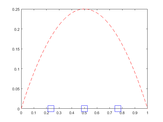
Figure 1: Final configuration of vehicle locations obtained by running the Lloyd descent algorithm. The red dashed line shows the density function $\phi(x)=x(1-x)$, while the blue squares denote the three vehicles.

In the second scenario, we consider the weight function $\phi(x):=x^{2}-x^{4}$ in the interval $[A,B]=[-W,W]$. Then, the polynomial $F(p,b,a)$ is given by

$$F(p,b,a)=\int_{a}^{b}(p-x)(x^{2}-x^{4})dx\\ =\frac{p}{3}(b^{3}-a^{3})-\frac{1}{4}(b^{4}-a^{4})-\frac{p}{5}(b^{5}-a^{5})+\frac{1}{6}(b^{6}-a^{6}).$$

Substituting into the system of equations (3.2), for the interval $[-W,W]$, we obtain

$$\frac{p_{1}}{3}\Big{(}\Big{(}\frac{p_{1}+p_{2}}{2}\Big{)}^{3}+W^{3}\Big{)}-\frac{1}{4}\Big{(}\Big{(}\frac{p_{1}+p_{2}}{2}\Big{)}^{4}-W^{4}\Big{)}$$

$$-\frac{p_{1}}{5}\Big{(}\Big{(}\frac{p_{1}+p_{2}}{2}\Big{)}^{5}+W^{5}\Big{)}+\frac{1}{6}\Big{(}\Big{(}\frac{p_{1}+p_{2}}{2}\Big{)}^{6}-W^{6}\Big{)}=0,$$

$$\frac{p_{2}}{3}\Big{(}\Big{(}\frac{p_{2}+p_{3}}{2}\Big{)}^{3}-\Big{(}\frac{p_{1}+p_{2}}{2}\Big{)}^{3}\Big{)}-\frac{1}{4}\Big{(}\Big{(}\frac{p_{2}+p_{3}}{2}\Big{)}^{4}-\Big{(}\frac{p_{1}+p_{2}}{2}\Big{)}^{4}\Big{)}$$

$$-\frac{p_{2}}{5}\Big{(}\Big{(}\frac{p_{2}+p_{3}}{2}\Big{)}^{5}-\Big{(}\frac{p_{1}+p_{2}}{2}\Big{)}^{5}\Big{)}+\frac{1}{6}\Big{(}\Big{(}\frac{p_{2}+p_{3}}{2}\Big{)}^{6}-\Big{(}\frac{p_{1}+p_{2}}{2}\Big{)}^{6}\Big{)}=0,$$

$$\frac{p_{3}}{3}\Big{(}W^{3}-\Big{(}\frac{p_{2}+p_{3}}{2}\Big{)}^{3}\Big{)}-\frac{1}{4}\Big{(}W^{4}-\Big{(}\frac{p_{2}+p_{3}}{2}\Big{)}^{4}\Big{)}$$

$$-\frac{p_{3}}{5}\Big{(}W^{5}-\Big{(}\frac{p_{2}+p_{3}}{2}\Big{)}^{5}\Big{)}+\frac{1}{6}\Big{(}W^{6}-\Big{(}\frac{p_{2}+p_{3}}{2}\Big{)}^{6}\Big{)}=0.$$ (7)

The system (7) also consists of three polynomial equations in three unknowns $p_{1},p_{2},p_{3}$. Using the technique from Section 4, we obtain a total of 122 solutions in $\mathbb{C}^{3}$, of which 30 are in $\mathbb{R}^{3}$. This computation yields that the global optimal solution is approximately $(-0.626,0.431,0.762)$. However, for this problem, from a class of initial configurations of the type $(-a,0,a)$, where $a\in(0,W)$, the Lloyd descent algorithm leads the vehicles toward a local minimum approximately at $(-0.66,0,0.66)$ as illustrated in Figure 2.

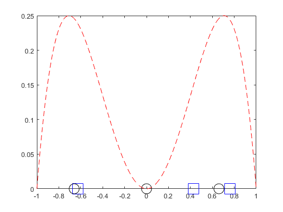
Figure 2: Final configuration of vehicle locations obtained by running the Lloyd descent algorithm. The red dashed line shows the density function $\phi(x)=-x^{4}+x^{2}$. The black circles denote the final output of the Lloyd algorithm when initialize from (-a, 0, a), while the blue squares denote the final output when the vehicles are initialized with a random initial configuration.

6 Conclusions and Future Directions

This paper considered the static coverage control problem for placement of vehicles with simple motion on the real line. We assumed that the cost is a polynomial function of the locations of the vehicles. Our main contribution was to demonstrate the use of a numerical polynomial homotopy continuation method that guarantees to find all solutions of polynomial equations, in order to characterize the global minima for the coverage control problem. The results were compared numerically using two examples with a classic distributed approach involving the use of Lloyd descent, known to converge only to a local minimum under certain technical conditions. We observed that in one of the examples, both methods lead to the same global minimizer, while in the second example, the Lloyd descent converges to only a local minimum when initialized from a particular class of configurations.

Future work is expected to center around fully distributed implementations of the polynomial homotopy method based on exploiting the structure of polynomials. We also plan to explore the complexity of this polynomial homotopy method in higher dimensional spaces.

References

- Al-Khateeb et al. (2009) Ashraf N. Al-Khateeb, Joseph M. Powers, Samuel Paolucci, Andrew J. Sommese, Jeffrey A. Diller, Jonathan D. Hauenstein, and Joshua D. Mengers. One-dimensional slow invariant manifolds for spatially homogenous reactive systems. The Journal of Chemical Physics, 131(2):024118, 2009.
- Bates et al. (2013) Daniel J. Bates, Jonathan D. Hauenstein, Andrew J. Sommese, and Charles W. Wampler. Numerically solving polynomial systems with Bertini, volume 25 of Software, Environments, and Tools. Society for Industrial and Applied Mathematics (SIAM), Philadelphia, PA, 2013.
- Bullo et al. (2009) Francesco Bullo, Jorge Cortes, and Sonia Martinez. Distributed control of robotic networks: a mathematical approach to motion coordination algorithms. Princeton University Press, 2009.
- Cortes et al. (2004) Jorge Cortes, Sonia Martinez, Timur Karatas, and Francesco Bullo. Coverage control for mobile sensing networks. IEEE Transactions on robotics and Automation, 20(2):243–255, 2004.
- Drezner and Hamacher (2001) Zvi Drezner and Horst W Hamacher. Facility location: applications and theory. Springer Science & Business Media, 2001.
- Du et al. (1999) Qiang Du, Vance Faber, and Max Gunzburger. Centroidal voronoi tessellations: Applications and algorithms. SIAM review, 41(4):637–676, 1999.
- Fekete et al. (2005) Sándor P Fekete, Joseph SB Mitchell, and Karin Beurer. On the continuous fermat-weber problem. Operations Research, 53(1):61–76, 2005.
- Girard et al. (2004) Anouck R Girard, Adam S Howell, and J Karl Hedrick. Border patrol and surveillance missions using multiple unmanned air vehicles. In Decision and Control, 2004. CDC. 43rd IEEE Conference on, volume 1, pages 620–625. IEEE, 2004.
- Gray and Neuhoff (1998) Robert M. Gray and David L. Neuhoff. Quantization. IEEE transactions on information theory, 44(6):2325–2383, 1998.
- Hauenstein et al. (2011) Jonathan D. Hauenstein, Andrew J. Sommese, and Charles W. Wampler. Regeneration homotopies for solving systems of polynomials. Math. Comp., 80(273):345–377, 2011.
- Kwok and Martínez (2010) Andrew Kwok and Sonia Martínez. A coverage algorithm for drifters in a river environment. In American Control Conference (ACC), 2010, pages 6436–6441. IEEE, 2010.
- Martínez and Bullo (2006) Sonia Martínez and Francesco Bullo. Optimal sensor placement and motion coordination for target tracking. Automatica, 42(4):661–668, 2006.
- Mehta et al. (2015) Dhagash Mehta, Noah S. Daleo, Florian Dörfler, and Jonathan D. Hauenstein. Algebraic geometrization of the Kuramoto model: equilibria and stability analysis. Chaos, 25(5):053103, 7, 2015.
- Schwager et al. (2009) Mac Schwager, Daniela Rus, and Jean-Jacques Slotine. Decentralized, adaptive coverage control for networked robots. The International Journal of Robotics Research, 28(3):357–375, 2009.
- Sommese and Wampler (2005) Andrew J. Sommese and Charles W. Wampler, II. The numerical solution of systems of polynomials arising in engineering and science. World Scientific Publishing Co. Pte. Ltd., Hackensack, NJ, 2005.
- Szechtman et al. (2008) Roberto Szechtman, Moshe Kress, Kyle Lin, and Dolev Cfir. Models of sensor operations for border surveillance. Naval Research Logistics (NRL), 55(1):27–41, 2008.
- Zemel (1985) Eitan Zemel. Probabilistic analysis of geometric location problems. SIAM Journal on Algebraic Discrete Methods, 6(2):189–200, 1985.