Two-dimensional vortex quantum droplets

Abstract

It was recently found that the Lee-Huang-Yang (LHY) correction to the mean-field Hamiltonian of binary atomic boson condensates suppresses the collapse and creates stable localized modes (two-component “quantum droplets”, QDs) in two and three dimensions (2D and 3D). In particular, the LHY effect modifies the effective Gross-Pitaevskii equation (GPE) in 2D by adding a logarithmic factor to the usual cubic term. In the framework of the accordingly modified two-component GPE system, we construct 2D self-trapped modes in the form of QDs with vorticity $S$ embedded into each component. Due to the effect of the logarithmic factor, the QDs feature a flat-top shape, which expands with the increase of $S$ and norm $N$. An essential finding, produced by a systematic numerical investigation and analytical estimates, is that the vortical QDs are stable (which is a critical issue for vortex solitons in nonlinear models) up to $S=5$, for $N$ exceeding a certain threshold value, which is predicted to scale as $N_{\mathrm{th}}\sim S^{4}$ for large $S$ (for three-dimensional QDs, the scaling is $N_{\mathrm{th}}\sim S^{6}$). The prediction is corroborated by numerical findings. Pivots of QDs with $S\geq 2$ are subject to structural instability, as specially selected perturbations can split the single pivot in a set of $S$ or $S+2$ pivots  corresponding to unitary vortices; however, the structural instability remains virtually invisible, as it occurs in a broad central “hole” of the vortex soliton, where values of fields are very small, and it does not cause any dynamical instability. In the condensate of ³⁹K atoms, in which QDs with $S=0$ and a quasi-2D shape were created recently, the vortical droplets may have radial size $\lesssim 30$ $\mathrm{\mu}$m, with the number of atoms in the range of $10^{4}-10^{5}$. The role of three-body losses is considered too, demonstrating that they do not prevent the creation of the vortex droplets, but may produce a noteworthy effect, leading to sudden splitting of “light” droplets. In addition, hidden-vorticity states in QDs, with topological charges $S_{+}=-S_{-}=1$ in their components, which are prone to strong instability in other settings, have their stability region too. Unstable HV states tend to spontaneously merge into zero-vorticity solitons. Collisions of QDs, which may lead to their merger, and dynamics of elliptically deformed QDs (which form rotating elongated patterns or ones with oscillations of the eccentricity) are briefly considered too.

I Introduction

The mean-field approximation GP1 ; GP2 offers an extremely accurate description of one-, two, and three-dimensional (1D, 2D, 3D) matter-wave patterns in atomic Bose-Einstein condensates (BECs), provided that the multidimensional states are not made unstable by the occurrence of the collapse review . However, the usual cubic nonlinearity, which represents attractive interactions between atoms, gives rise to the critical and supercritical collapse in the 2D and 3D geometries, respectively Berge' ; Fibich , which makes search for physically relevant mechanisms stabilizing 2D and 3D solitons and solitary vortices a challenging problem review ; review2 . If the physical setting admits the inclusion of repulsive quintic nonlinearity in addition to the cubic self-focusing, the balance of these terms stabilizes 2D and 3D fundamental solitons, with vorticity $S=0$, as well as a part of 2D and 3D vortex-soliton families, with $S\geq 1$ Spain ; Pego ; Kiev and $S=1$ 3D-vortex , respectively. The stabilization of fundamental 2D solitons by the cubic-quintic nonlinearity has been experimentally demonstrated in optics Cid , while quasi-stable solitary vortices were demonstrated only as transient modes, using the instability-suppressing effect of the cubic loss (two-photon absorption) Cid2 . However, the relevance of the cubic-quintic nonlinearity in the context of BEC is doubtful. A recently found possibility to create 2D vortex solitons, which are stable, at least, up to $S=5$, was predicted in the framework of the binary BEC with its two components coupled by a microwave field Jqing2016 . Stabilization of higher-order vortices with $S>1$ is an especially interesting issue in this and other contexts.

It was also recently found that the spin-orbit coupling in binary BECs with the cubic attraction makes otherwise unstable 2D solitons an absolutely stable ground state BenLi ; Luca ; Yongyao2017 , and creates metastable solitons in 3D HanPu ; SKA . However, all modes with overall vorticity $S\geq 1$ added to them are completely unstable in the spin-orbit-coupled system BenLi . Thus far, no truly stable bright vortex solitons have been created experimentally in any uniform physical medium or in free space review ; review2 (it may be easier to create 3D modes with embedded vorticity in deeply structured media, such as quasi-discrete “optical bullets” in a 2D waveguiding array Jena ).

A new approach to the creation of stable self-trapped 2D and 3D states in the BEC was recently elaborated in Refs. Petrov2015 ; Petrov2016 in a binary BEC, with self-repulsion in each component and dominating inter-component attraction. In this setting, the stability against the collapse is provided by the Lee-Huang-Yang (LHY) correction to the mean-field dynamics, originating from quantum fluctuations around the mean-field states LHY1957 . In terms of the respective 3D Gross-Pitaevskii equations (GPEs), the LHY correction is represented by quartic self-repulsive terms, which arrest the collapse induced by the cross-attraction between the components Petrov2015 (or by the three-body attraction in 1D Sekino2018 ). The analysis predicts stable quantum droplets (QDs) of an ultradilute superfluid, while traditional solitons in BEC were created as quantum-gas clouds Randy -Aspect . A variant of this system, which includes the linear Rabi coupling between the components, was considered too Luca2 . The interplay of the LHY and spin-orbit-coupling effects was addressed in Refs. Zhengwei2013 , Yongyao2017 , and new (the latter work applied these ingredients to a Bose-Fermi mixture).

Beyond the framework of the corrected mean-field theory, the zero-vorticity QDs and their stability were recently explored, by means of the quantum Monte-Carlo method in Ref. Boronat , and the stability of uniform media filling broad “droplets” was studied, by means of nonperturbative treatment of correlations, in Ref. Zillich . Further, beyond-the-mean-field theory valid at finite temperature was recently developed too Chiquillo .

QDs have been created in the binary BEC composed of $10^{4}-10^{5}$ atoms of ³⁹K, kept in two different states, with appropriate signs of the inter- and intra-component interactions Cabrera2017 -Inguscio (the corresponding scattering lengths in ³⁹K may be adjusted by the Feshbach resonance FR1 ; FR2 ). In particular, in works Cabrera2017 and Cabrera2 the QDs were produced  with a quasi-2D (“pancake”) shape, imposed by the strong confining potential applied perpendicular to the pancake’s plane. On the other hand, the QDs reported in Ref. Inguscio were nearly isotropic (spherically symmetric), as they were not essentially compressed by the confining potential.

Another possibility for the creation of QDs was realized in dipolar BEC, where the balance of attractive dipole-dipole interactions and LHY repulsion makes it possible to create single-component QD states, as demonstrated, using ¹⁶⁴Dy and ¹⁶⁶Er condensates, in Refs. Barbut2016 and Schmitt2016 , respectively. The dynamics of QDs in dipolar BECs was analyzed in detail in recent works PRX -Sadhan .

The availability of QDs in the current experiments suggests to analyze a possibility of the creation of such states with embedded vorticity. In single-component dipolar condensates, the vortex states were recently found to be unstable, because deformation of the vortex embedded in the QD may lower its energy Macri . On the other hand, it was demonstrated, also very recently, that two-component QDs supported by the contact interactions in 3D may readily carry stable embedded vorticities with winding number $S=1$, and the QDs with very large norms may also support stable embedded vorticity $S=2$ Leticia .

The objective of the present work is to construct families of stable QDs with embedded vorticity in the effectively 2D setting. The reduction of the dimension from 3 to 2 changes the form of the nonlinearity in the underlying Gross-Pitaevskii equations (GPEs) including the LHY correction Petrov2016 , and thus gives rise to a specific model in the framework of which the analysis produces vortex solitons. A remarkable fact is that conspicuous stability regions are found for the solitons with vorticities up to $S=5$.

The paper is structured as follows. The model is introduced in Sec. II. Basic results for QDs with explicit and “hidden” vorticities are presented in Sec. III [“hidden” means that two components of the QD have equal norms and opposite vorticities, see Eq. (30) below]. In addition to systematically collected numerical findings, essential analytical results are reported too. They include estimates for the size of the inner “hole” of the QDs, induced by the vorticity, and threshold (minimum) value of the norm necessary for the stability of the vortex QDs, in the form of $N_{\mathrm{th}}\sim S^{4}$ [for three-dimensional vortex QDs, it is replaced by $N_{\mathrm{th}}(S)\sim S^{6}$]. Another feature predicted by the analytical approach and confirmed numerically is the effect of the structural instability of the multiple vortices, with $S>1$: while the vortex QD as a whole remains stable, small perturbations, with their own intrinsic vorticities $s=+1$ and $s=-1$, split the pivot of the multiple vortex in a set of unitary ones, with the number of secondary pivots being, respectively, $S$ or $S+2$. The split pivots stay close to each other, without initiating the growth of a dynamical instability. Estimates for experimentally relevant parameters of the predicted stable modes, along with analysis an effect of cubic loss, which may also be an experimentally relevant factor, are given in Sec. V. Collisions between QDs, as well as dynamics of elliptically deformed ones, are briefly addressed in Sec. VI. The paper is concluded by Sec. VII.

II The model

The binary BEC in 3D is governed by the GPE system with the cubic terms, supplemented by the above-mentioned LHY-induced quartic self-repulsion Petrov2016 . For the quasi-2D BEC, strongly confined in the transverse direction, the GPE-LHY system reduces to a 2D form Petrov2016 , which essentially simplifies for modes with lateral size $l\gg\sqrt{a_{\pm}a_{\perp}}$, where $a_{\pm}$ and $a_{\perp}$ are, respectively, the self-repulsion scattering lengths of each component, and the transverse-confinement length Yongyao2017 . This condition definitely holds for values relevant to the current experiments, $l\sim 10$ $\mathrm{\mu}$m, $a_{\pm}\sim 3$ nm, $a_{\perp}\lesssim 1$ $\mathrm{\mu}$m Cabrera2017 ; Inguscio ; Cabrera2 , leading to the reduced 2D system for scaled wave functions $\psi_{\pm}$ of the two components Petrov2016 ; Yongyao2017 , with coordinates and time additionally rescaled by $\left(x,y\right)\rightarrow\left(g/2\sqrt{\pi}\right)\left(x,y\right),t\rightarrow\left(g^{2}/4\pi\right)t$:

$$i\frac{\partial\psi_{\pm}}{\partial t}=-\frac{{1}}{2}\nabla^{2}\psi_{\pm}+\frac{4\pi}{g}(|\psi_{\pm}|^{2}-|\psi_{\mp}|^{2})\psi_{\pm}$$

$$+\left(|\psi_{+}|^{2}+|\psi_{-}|^{2}\right)\psi_{\pm}\ln(|\psi_{+}|^{2}+|\psi_{-}|^{2})-iL_{3}|\psi_{\pm}|^{4}\psi_{\pm},$$ (1)

where $g>0$ is the coupling constant, and the symmetry between the components is assumed, $a_{+}=a_{-}$. In the experimental situation, the latter condition holds only approximately (in particular, in the setting reported in Ref. Cabrera2017 , the relative difference between $a_{+}$ and $a_{-}$ is $\simeq 20\%$ at magnetic fields close to $55.5$ G). Here, we focus on the symmetric system as the simplest one which may be close enough to the experiment (cf. Refs. Petrov2015 and Petrov2016 ), while the detailed analysis of the asymmetric system should be a subject for a separate work. Further, $L_{3}$ in Eq. (1) is the scaled rate of three-body losses, which should be taken into account in the realistic situation Cabrera2017 ; Inguscio ; Cabrera2 .

For symmetric states with

$$\psi_{+}=\psi_{-}\equiv\psi/\sqrt{2},$$ (2)

system (1) admits reduction to a single equation,

$$i\frac{\partial\psi}{\partial t}=-\frac{{1}}{2}\nabla^{2}\psi+|\psi|^{2}\psi\ln(|\psi|^{2})-i\frac{L_{3}}{4}|\psi|^{4}\psi.$$ (3)

The symmetric states are characterized by the total norm, $N=\int\int|\psi(\mathbf{r})|^{2}dxdy$ (it is subject to slow decay under the action of the loss, if the latter is present). In the case of $L_{3}=0$, the Hamiltonian (energy) corresponding to Eq. (3) is

$$E=\frac{{1}}{2}\int\int\left[\left|\nabla\psi\right|^{2}+|\psi|^{4}\ln\left(\frac{|\psi|^{2}}{\sqrt{e}}\right)\right]dxdy$$ (4)

($e$ is the base of natural logarithms). Equation (3) with $L_{4}=0$ also conserves the linear and angular momenta: $\mathbf{P}=i\int\int\psi^{\ast}\nabla\psi dxdy$, and

$$M=i\int\int\psi^{\ast}\left(y\frac{\partial\psi}{\partial x}-x\frac{\partial\psi}{\partial y}\right)dxdy\equiv i\int\int\psi^{\ast}\frac{\partial\psi}{\partial\theta}dxdy,$$ (5)

where $\ast$ stands for the complex conjugation, and $\left(r,\theta\right)$ is the set of the polar coordinates in the $\left(x,y\right)$ plane.

Our first objective is to construct 2D self-trapped modes with embedded vorticity, and explore their stability, in the lossless model with $L_{3}=0$ (previously, only zero-vorticity 2D solutions, whose stability is obvious, were addressed in the context of the QD models Petrov2016 ); then, the effect of the three-body loss will be considered. This objective is relevant as the droplets created in recent works Cabrera2017 ; Cabrera2 feature a strongly oblate form, with the ratio of the radial and transverse sizes $\gtrsim 10$.

QD solutions to Eq. (3), with vorticities $S=0,1,2,...$ , are looked for, in the polar coordinates, as

$$\psi(\mathbf{r},t)=\phi(r)\exp\left(-i\mu t+iS\theta\right),$$ (6)

where $\mu<0$ is a chemical potential, and real amplitude function $\phi(r)$ obeys a radial equation (with $L_{3}=0$),

$$\mu\phi=-\frac{1}{2}\left(\frac{d^{2}\phi}{dr^{2}}+\frac{1}{r}\frac{d\phi}{dr}-\frac{S^{2}}{r^{2}}\phi\right)+\phi^{3}\ln\left(\phi^{2}\right).$$ (7)

Note that, as it follows from Eq. (5), the angular momentum of QD (6) (its “spin momentum”) is proportional to its integral norm,

$$M_{\mathrm{spin}}=SN.$$ (8)

The same equation (7) describes the radial structure of two-component QDs with hidden vorticity (HV), in the form of $\psi_{\pm}(\mathbf{r},t)=\phi(r)\exp\left(-i\mu t\pm iS\theta\right)$ hidden , although their stability is completely different, as shown below, and their total angular momentum is zero (hence the name of “hidden vorticity”).

Localized solutions of Eq. (7) with fixed $N$ and $S$ were obtained by means of the imaginary-time-integration method (which may work for vortex configurations as well as for ground states IT1 ; IT2 ), applied to Eq. (3) with $L_{3}=0$ and input $\phi_{0}(\mathbf{r})=Cr^{S}\exp(-\alpha r^{2}+iS\theta),$ $\alpha>0$. The stability of the stationary modes was analyzed by means of the linearized Bogoliubov - de Gennes (BdG) equations GP1 ; GP2 for perturbed wave functions, taken as

$$\psi_{\pm}=\left[\phi_{\pm}(r)+w_{\pm}e^{-i\Lambda t+im\theta}+v_{\pm}^{\ast}e^{i\Lambda^{\ast}t-im\theta}\right]e^{-i\mu t+iS\theta},$$ (9)

where $w_{\pm}$ and $v_{\pm}$ are perturbation eigenmodes with integer azimuthal index $m$, and the imaginary part of eigenvalue $\Lambda$ determines the instability growth rate, if any (see, e.g., Ref. VS ). Note that perturbations which break the symmetry of the underlying states [see Eq. (2)] are admitted by Eq. (9). The system of BdG equations was derived in a straightforward manner, by the substitution of perturbed wave functions (9) in Eq. (1) and subsequent linearization. Numerical solution of the linearized equations produces a spectrum of eigenfrequencies $\Lambda$, the stability condition being that they all must be real. The so predicted (in)stability was then verified by direct simulations of the perturbed evolution in the framework of Eq. (1), again admitting perturbations which may break the symmetry relation imposed by Eq. (2).

III Results

III.1 Zero-vorticity solitons and the flat-top state

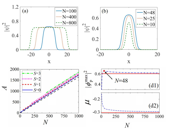
Figure 1: (a) Cross-sections of density patterns $|\phi(\mathbf{r})|^{2}$ for the QDs of the flat-top type with $S=0$ (the system’s ground state) and norms $N=100$ (solid curve), $400$ (dot curve), and $800$ (dash curve). (b) Cross-sections of density patterns $|\phi(\mathbf{r})|^{2}$ for the QDs of the Gaussian type with $S=0$ (the system’s ground state) and norms $N=10$ (dash curve), $25$ (dot curve), and $48$ (solid curve). (c) The effective area (10) for QDs with embedded vorticities $S=0$ (solid line) ,1 (short dash line),2 (dot line),3 (dash-dot line), vs. $N$. The long dashed line represents the TF prediction, $A=N/n_{\mathrm{p}}^{\mathrm{(TF)}}$ for $S=0$, see Eq. (11). (d1,d2) The largest (peak) local density, $|\phi_{\mathrm{p}}|^{2}\equiv n_{\mathrm{p}}$ [dash-dot curve in panel (d1)], and chemical potential $\mu$ [dash-dot curve in penal (d2)] vs. $N$. Solid lines in these two panels show the TF limit values, $n_{\mathrm{p}}^{\mathrm{(TF)}}=1/\sqrt{e}$ and $\mu_{\mathrm{TF}}=-1/\left(2\sqrt{e}\right)$, see Eqs. (13) and (14), respectively. The rhombus in panel (d1) designates the border between the QD profiles of the Gaussian and flat-top types.

The analysis demonstrates that all the QDs with $S=0$, which represent the ground state of the system, are stable. Similar to the situation with 1D QDs Grisha , they feature quasi-Gaussian and flat-top shapes at relatively small and larger norms ($N<48$  and $N>48$, respectively), as shown in Fig. 1. Their effective area,

$$A\equiv\left[\int|\phi(\mathbf{r})|^{4}d\mathbf{r}\right]^{-1}\left(\int|\phi(\mathbf{r})|^{2}d\mathbf{r}\right)^{2},$$ (10)

is displayed, as a function of norm $N$, along with the peak local density, $|\psi\left(\mathbf{r}=0\right)|^{2}$, and chemical potential $\mu$, in Fig. 1. The border between the quasi-Gaussian and flat-top shapes [designated by the the red rhombus at $N=48$ in Fig. 1(d1)] corresponds to the maximum of the peak density. In this and other figures,the length and time units correspond to $\sim 1$ $\mathrm{\mu}$m and $\sim 1$ ms respectively, with $N=100$ corresponding to $\sim 5000$ atoms, in terms of the ³⁹K condensate Cabrera2017 ; Cabrera2 . Note that the $\mu(N)$ curve satisfies the necessary stability condition in the form of the Vakhitov-Kolokolov criterion VK ; Berge' ; Fibich , $d\mu/dN<0$.

The flat-top structure of fundamental and vortical solitons (for norms which are not too small) is demonstrated by models which include competing self-attraction and repulsion terms, such as the nonlinear Schrödinger equations with cubic-quintic Pushka ; Enns ; Spain ; Pego , cubic-quartic Leticia and quadratic-cubic Grisha nonlinearities. This feature is demonstrated by the solitons in one Pushka ; Enns ; Grisha ; Luca3 , two Spain ; Pego and three Leticia dimensions alike. However, in the present system the reason is different, as Eq. (7) includes a single nonlinear term, $\phi^{3}\ln\left(\phi^{2}\right)$. This term switches its sign from attraction to repulsion due to the reversal of the sign of $\ln\left(\phi^{2}\right)$ as its argument changes from $\phi^{2}<1$ to $\phi^{2}>1$. This mechanism arrests the critical collapse Berge' ; Fibich in the present 2D system, driven by the cubic self-attraction, and, thus, it suggests the possibility of the existence of stable solitons.

The flat-top states may be analyzed, first, by means of the Thomas-Fermi (TF) approximation, which neglects the derivatives in Eq. (7) with $S=0$. The respective energy density of the flat field, which carries the peak (largest) density, $n_{\mathrm{p}}\equiv|\phi_{\mathrm{p}}|^{2}$, of the QD profile [see Fig. 1(a)] is $\epsilon(n_{\mathrm{p}})=n_{\mathrm{p}}^{2}\ln(n_{\mathrm{p}}/\sqrt{e})$, as per Eq. (4). With area

$$A\approx N/n_{\mathrm{p}}$$ (11)

of the flat-top QD, its bulk energy, which dominates the total energy (4), is

$$E_{\mathrm{bulk}}\approx A\epsilon(n_{\mathrm{p}})=Nn_{\mathrm{p}}\ln(n_{\mathrm{p}}/\sqrt{e}).$$ (12)

Then, $n_{\mathrm{p}}$ is determined by the minimization of the energy for the given norm: $dE/dn_{\mathrm{p}}=0$, yielding

$$n_{\mathrm{p}}^{\mathrm{(TF)}}=1/\sqrt{e}\approx 0.6065,$$ (13)

which is very close to the numerically found values, see Fig. 1(c) [and Fig. 3(b1) below]. The respective chemical potential is

$$\mu_{\mathrm{TF}}=n_{\mathrm{p}}^{\mathrm{(TF)}}\ln(n_{\mathrm{p}}^{\mathrm{(TF)}})=-1/\left(2\sqrt{e}\right)\approx-0.3033,$$ (14)

in agreement with numerical data displayed in Figs. 1(d2) and 3(b2).

The same results for the peak density and chemical potential can also be obtained in a different way. Indeed, for broad flat-top QDs, radial equation (7) becomes quasi-one-dimensional,

$$\mu\phi=-\frac{1}{2}\frac{d^{2}\phi}{dr^{2}}+\phi^{3}\ln\left(\phi^{2}\right).$$ (15)

The respective formal Hamiltonian, which remains constant in the course of the spatial evolution of the field along $r$, is

$$h=\frac{\mu}{2}\phi^{2}+\frac{1}{4}\left(\frac{d\phi}{dr}\right)^{2}-\frac{1}{4}\phi^{4}\ln\left(\frac{\phi^{2}}{\sqrt{e}}\right).$$ (16)

For localized QDs with $\phi(r=\infty)=0$, one should set $h=0$ in Eq. (16). Finally, in the limit of very broad QDs the derivative terms in Eqs. (15) and (16) may be dropped, which yields an algebraic system, $\mu=\phi^{2}\ln\left(\phi^{2}\right),~{}\mu=(1/2)\phi^{2}\ln\left(\phi^{2}/\sqrt{e}\right)$. A solution of this system is identical to the values given by Eqs. (13) and (14).

III.2 Vortex solitons

III.2.1 The shape

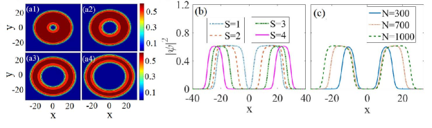
Figure 2: Panels (a1)-(a4) display density patterns of vortex QDs with $S=1$,$2$, $3$, $4$ and norm $N=1000$. The first three QDs are stable, while the one corresponding to $S=4$ is not, see Fig. 3(a2). (b) Cross-sections of the density patterns from panels (a1)-(a4) (dot, dash, dash-dot, and solid curves represent $S=1$, 2, 3, and 4, respectively). (c) The same as in (b), for $S=1$ and different values of $N$ (solid, dot and dash curves represent $N=300$, 700, and 1000, respectively). All vortex QDs shown in (c) are stable.

Typical examples of numerically found vortex QDs with $N=1000$ are displayed in Figs. 2(a,b), which shows that they are flat-top rings, with inner and outer radii growing with the increase of $S$. The inner radius can be roughly predicted using the TF approximation (which may be relevant for vortices Feder ), applied to Eq. (7). This yields either $\phi=0$ or

$$\mu-\phi^{2}\ln\left(\phi^{2}\right)=\frac{S^{2}}{2r^{2}}.$$ (17)

Equation (17) shows that $\phi(r)$ keeps decreasing, following the decrease of $r$ towards $r=0$, up to $\phi_{\min}=1/\sqrt{e}$. Substituting here $\phi=\phi_{\min}$ and $\mu=\mu_{\mathrm{TF}}$ from Eq. (14), we find that $\phi=\phi_{\min}$ is attained at

$$r_{\min}=\sqrt{e/(2-\sqrt{e})}S\approx 2.8S.$$ (18)

At $r<r_{\min}$, the TF solution given by Eq. (17) cannot be used, hence it jumps to $\phi=0$. Thus, $r_{\min}$ can be used as an estimate for the radius of the inner “hole” of the vortex soliton.

The area of the vortex QDs, defined as per Eq. (10), is shown, as a function of $N$, in Fig. 1(c), which implies that it is well estimated, as above, by relation $A=\sqrt{e}N$, that directly follows from Eqs. (11) and (13). Further, Figs. 2 and 3(a1) demonstrates that the vortex’ internal radius grows quasi-linearly with $S$ and does not depend on $N$, as predicted by Eq. (18), the numerically found values of the radius being relatively close to those given by Eq. (18). Figures 3(b1,b2) demonstrate that, with the increase of $N$, the peak density of vortex rings quickly tends to the TF limit value given by Eq. (13), while the chemical potential approaches the respective limit, given by Eq. (14), much slower, due to the contribution of the vorticity.

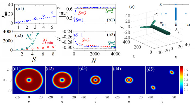
Figure 3: (a1) The numerically found radius of the vortex’ inner hole vs. $S$ [each point corresponds to $N_{\mathrm{th}}(S)$ in panel (a2)], the dashed line showing the prediction given by the TF approximation, according to Eq. (18). (a2) Minimum norms, $N_{\min}$, necessary for the existence of the vortex QDs (circles), and threshold values of the norm necessary for their stability, $N_{\mathrm{th}}$ (triangles), vs $S$. The dashed curve shows the fit to analytically predicted scaling (24), $N_{\mathrm{th}}=6S^{4}$. Numerically exact values of $N_{\min}(S)$ and $N_{\mathrm{th}}(S)$ are additionally produced in Table 1. (b1,b2) The peak density and chemical potential of QDs with different vorticities, vs. $N$ (dash-dot, dash, and solid curves represent $S=1$, 3, and 5, respectively ). Horizontal dot lines show the TF-predicted limit values $n_{\mathrm{p}}^{\mathrm{(TF)}}$ and $\mu_{\mathrm{TF}}$, see Eqs. (13) and (14), respectively. (c) The evolution of an unstable QD with $(N,S)=(30,1)$. The inset shows the respective spectrum of stability eigenvalues $\Lambda$. The above panels pertain to $L_{3}=0$ (no three-body loss). (d) The evolution of the density pattern of the QD with $S=1$ and initial norm $N=1000$, produced by simulations of Eq. (3) with $L_{3}=0.01$, starting from $t=0$ (d1). Other plots pertain to $t=464$ (d2), $1584$ (d3), $3008$ and $3120$ (d4,d5).

III.2.2 Dynamical stability: numerical results and analytical estimates

To address the stability of the vortices, we first note that, if they are shaped as relatively narrow annuli (see Fig. 2), it is possible to produce an estimate based on the consideration of the azimuthal modulational instability (MI) in the 1D reduction of Eq. (1) for the narrow ring; we stress that this consideration admits perturbations violating the equality between the components, see Eq. (2). The result is that MI does not occur if the density is large enough, $n\equiv|\psi|^{2}>1/e\approx 0.6~{}n_{\mathrm{p}}^{\mathrm{(TF)}}$. Coupling constant $g$ from Eq. (1) does not appear in this condition, suggesting that the full stability may be insensitive to $g$. For the HV states the analysis produces a more restrictive condition for the absence of MI, which includes $g$: $\left(n-\pi gS^{2}/R^{2}\right)\ln\left(en\right)>\left(2\pi S/R\right)^{2}$, where $R$ is the ring’s radius, suggesting that HV modes are more prone to instability, depending on the value of $g$. These qualitative predictions are confirmed by numerical results reported below.

Data produced by the numerical solution of the linearized equations for eigenmodes of small perturbations, and fully confirmed by direct simulations of the perturbed evolution (not shown here in detail), reveal that vortex QDs in the system without the three-body loss exist above a minimum value of the norm, $N>N_{\min}$ [which is not surprising, as, in the framework of the cubic GPE, (unstable) 2D solitons with each value of $S$ exist at a single value of $N$ Berge' ; Fibich ], and they are stable above a certain threshold  value, i.e., at $N>N_{\mathrm{th}}>N_{\min}$, see Fig. 3(a2), which shows that $N_{\mathrm{th}}$ steeply grows with $S$. As a result, stable vortices were found up to $S=5$, but not for $S\geq 6$. In this connection, it is relevant to mention that the recent analysis of the three-dimensional QD model has revealed stability solely for $S=1$ and $2$, with an extremely large  $N_{\mathrm{th}}(S=2)$ Leticia . In addition to Fig. 3(a2), numerically exact values of $N_{\min}$ and $N_{\mathrm{th}}$ are collected in Table 1.

$S$	$1$	$2$	$3$	$4$	$5$
$N_{\min}$	$25$	$100$	$260$	$340$	$450$
$N_{\mathrm{th}}$	$60$	$200$	$510$	$1380$	$3550$

Table 1: numerically exact values of lower boundaries in terms of the norm, necessary for the existence ($N_{\min}$) and stability ($N_{\mathrm{th}}$) of vortex QDs with winding number $S$. The same data are displayed graphically in Fig. 3(a2).

In the interval of $N_{\min}<N<N_{\mathrm{th}}$, unstable vortices with winding number $S$ split, typically, into $S+1$ fragments, see an example for $S=1$ (splitting into a pair of fragments, each being, approximately. a zero-vorticity soliton) in Fig. 3(c). Splitting is a typical outcome of the evolution of unstable vortex solitons in previously studied models Spain -Kiev , hidden .

We stress that, although the full GPE-LHY system (1) contains coupling constant $g$, the stability boundary, $N_{\mathrm{th}}(S)$, does not depend on $g$ (in agreement with the above-mentioned prediction produced by the azimuthal-MI analysis), i.e., $N_{\mathrm{th}}(S)$ is determined by the analysis performed in the framework of Eq. (3), from which $g$ was scaled out, while perturbations breaking the symmetry constraint (2), which reduces Eq. (1) to Eq. (3), do not introduce additional instabilities.

The dependence of $N_{\mathrm{th}}$ on $S$ can be explained by means of an analytical approximation, based on the energy estimate for the vortex QDs of a large radius, $R$ (i.e., with a large norm, $N$), cf. a similar estimate for the 3D vortical QDs developed in Ref. Leticia . Indeed, the splitting of the flat-top vortical QD in two or several fundamental solitons, which also feature the flat-top shape, in the first approximation does not alter the bulk energy, which is proportional to the conserved total norm of the solitons, as per Eq. (12). Then, the stability against the splitting is determined by the balance of three other terms: the surface energy, $E_{\mathrm{surf}}$, the vortical (phase-gradient) energy of the unsplit vortex, $E_{\mathrm{vort}}$, and the kinetic energy of the splinters, $E_{\mathrm{kin}}$, which is determined by the conservation of the angular momentum.

First, taking into regard that radius $r_{\min}$ of the inner “hole” in the first approximation does not depend on the outer radius, $R$, the contribution of the hole’s edge to $E_{\mathrm{surf}}$ is negligible in comparison with that of the outer edge, for $R\gg r_{\min}$. Thus, one concludes that, in the simplest case of the splitting of the vortical soliton of radius $R$ in two fundamental ones [as in Fig. 3(c)], radii of the splinters are determined by the conservation of the total norm:

$$R_{\mathrm{splinter}}=R/\sqrt{2}.$$ (19)

Then, the resultant splitting-induced increase of the surface energy is

$$\Delta E_{\mathrm{surf}}=2\pi\sigma\left(\sqrt{2}-1\right)R,$$ (20)

where $\sigma$ is an efficient surface tension, which is a fixed constant for flat-top solitons with the fixed density, close to one given by Eq. (13).

The vortical-energy term in total Hamiltonian (4) may be readily estimated as

$$E_{\mathrm{vort}}=\pi\int_{0}^{\infty}\left|\frac{\partial\psi}{\partial\theta}\right|^{2}\frac{dr}{r}\approx\pi S^{2}n_{\mathrm{p}}\ln\left(\frac{R}{r_{\min}}\right).$$ (21)

Lastly, assuming that the two splinters emerge being separated by distance equal to their diameter, i.e., $2R_{\mathrm{splinter}}=\sqrt{2}R$, pursuant to Eq. (19), and they start to move with velocities $\pm V$ in opposite directions, $V$ can be estimated by equating the respective orbital momentum, $M_{\mathrm{orbit}}=\sqrt{2}RVN$ (the soliton’s dynamical mass is equal to its norm) to the original “spin” momentum (8): $V=S/\left(\sqrt{2}R\right)$. Thus, the kinetic energy of the emerging soliton pair is

$$E_{\mathrm{kin}}=\frac{1}{2}NV^{2}\equiv\frac{\pi}{4}n_{\mathrm{p}}S^{2},$$ (22)

where the norm was substituted by

$$N=\pi R^{2}n_{\mathrm{p}},$$ (23)

as per Eq. (11). Analyzing the energy balance for the possible splitting of the vortex solitons with large $R$, in the lowest approximation one may neglect $R$-independent term (22) in comparison with those given by Eqs. (20) and (21), which are growing functions of $R$.

Thus, the stability against the splitting may be predicted for (large) values of $R$ at which, for given (sufficiently large) $S$, the splitting-induced increase of the surface energy, estimated by Eq. (20), exceeds the energy drop due to the disappearance of the vortical energy, which is given by Eq. (21): $\Delta E_{\mathrm{surf}}(R)\geq E_{\mathrm{vort}}(R)$. Substituting here expressions (20) and (21), and taking into regard that $\ln\left(R/r_{\min}\right)$ is a slowly varying function of its argument, the stability boundary (threshold value of the norm) corresponds to the following scaling relation:

$$N\geq N_{\mathrm{th}}\simeq\mathrm{const}\cdot S^{4},$$ (24)

where Eq. (23) was used to eliminate $R$ in favor of $N$. As shown in Fig. (3(a2), Eq. (24), with a properly adjusted value of $\mathrm{const}$, provides quite an accurate fit to the numerically found dependence $N_{\mathrm{th}}(S)$. It is worthy to mention that this consideration is quite general, and the asymptotic scaling given by Eq. (24) should apply to other 2D models which support stable vortex solitons with the flat-top shape. For three-dimensional QDs with embedded vorticity, a similar approximation, which extends that developed in Ref. Leticia for $S=1$, yields $N_{\mathrm{th}}^{\mathrm{(3D)}}\simeq\mathrm{const}\cdot S^{6}$. This very steep dependence explains why the stability for three-dimensional vortex QDs was found only for $S=1$, and also for $S=2$ with extremely large values of $N$, but not for $S>2$.

Profiles of vortex QDs with $S=1,2,3,4$, selected precisely at the stability boundary, are displayed in Fig. 4. It is observed that their shape indeed develops towards the flat-top pattern with the increase of $S$, cf. typical patterns of the vortex states found in the depth of the stability area, which are displayed in Fig. 2 [except for the state with $S=4$ in Figs. 2(a,b), which is still unstable, as its norm falls slightly below $N_{\mathrm{th}}(S=4)$].

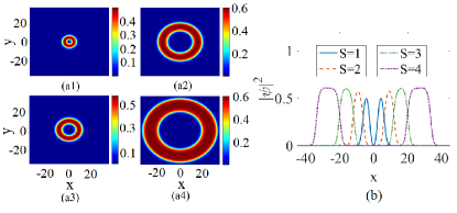
Figure 4: Panels (a1)-(a4) display density patterns of vortex QDs with $S=1$,$2$,$3$ and $4$ and norms $N=60$, $200$, $510$ and $1380$, respectively, which are selected from the stability boundary of the QDs, see Fig. 3(a2). (b) Cross-sections of the density patterns from panels (a1)-(a4).

III.2.3 Structural instability of higher-order vortex solitons

While, as shown above, solutions for QDs with multiple vorticity, up to $S=5$, can be easily found as stable ones, that are actually very robust against relatively strong perturbations, it is relevant to mention that all the higher-order vortices, with $S>1$, demonstrate structural instability, which implies that a specially selected small perturbation, without causing any dynamical instability, may split the pivot of the $S$-multiple vortex into sets of $S$ or $S+2$ pivots corresponding to unitary vortices, although the splitting remains almost invisible, as it occurs in the broad central “hole” induced by the multiple vorticity, where values of the wave fields remain extremely small. In fact, this structural instability is not specific to the current model, but is quite a generic effect, therefore we aim to briefly present it here in an explicit form.

In a small vicinity of the pivot of  a multiple vortex with $S\geq 2$, placed at the origin ($x=y=0$), a small disturbance with relative amplitude $-\varepsilon$ (generally, a complex one), which carries vorticity $s=1$, may be added, producing a perturbed configuration,

$$\psi_{\mathrm{pert}}\left(x,y\right)\approx\left(x+iy\right)^{S}-\varepsilon\left(x+iy\right)$$

$$\equiv \left(x+iy\right)\left[\left(x+iy\right)^{S-1}-\varepsilon\right].$$

Pivots of individual (unitary) vortices, into which the small disturbance splits the multiple vortex, are zeros of $\left|\psi_{\mathrm{pert}}\left(x,y\right)\right|$.  As seen from Eq. (9), these are points

$$x_{\mathrm{piv}}^{(1)}=y_{\mathrm{piv}}^{(1)}=0,$$ (26)

and $\left(S-1\right)$ additional points, determined as $\left(S-1\right)$ branches of the root of degree $1/\left(S-1\right)$:

$$x_{\mathrm{piv}}^{(1+j)}+iy_{\mathrm{piv}}^{(1+j)}=\varepsilon^{1/(S-1)},$$ (27)

where $j$ takes values $1,...,S-1$.

Another possibility is to consider a small disturbance with vorticity $s=-1$ (rather than $+1$, as considered above):

$$\psi_{\mathrm{pert}}\left(x,y\right)=\left(x+iy\right)^{S}-\varepsilon\left(x-iy\right).$$ (28)

In this case, the pivots are located at points defined by equation $\left(x+iy\right)^{S}=\varepsilon\left(x-iy\right)$, i.e., $\left(x+iy\right)^{S+1}=\varepsilon r^{2}$. After simple manipulations, the latter equation yields a set of $S+2$ pivots:

$$x_{\mathrm{piv}}^{(k)}+iy_{\mathrm{piv}}^{(k)}=\varepsilon^{1/(S+1)}\left|\varepsilon\right|^{2/\left(S^{2}-1\right)},$$ (29)

where $k$ takes values $1,...,S+1$, plus the central pivot defined by Eq. (26).

These simple arguments were verified by direct simulations, as shown in Fig. 5. Strong magnification of numerical data in the nearly empty area of the central “hole” precisely confirms the splitting of the $S$-multiple pivot into $S$ or $S+2$ sets of unitary-vortex pivots, under the action of the small initial perturbation with its own vorticity $s=+1$ or $s=-1$, respectively. Note that the original vortex with $S=1$ is not subject to the splitting in either case. It is also relevant to stress that the splitting remains virtually invisible on the normal scale of $\left|\psi\left(x,y\right)\right|$, hence it does not imply any conspicuous instability of the solitons carrying the multiple vorticity.

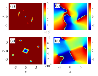
Figure 5: (a) A zoom (in domain $\left|x,y\right|\leq 8$) of the density pattern, $\left|\psi\left(x,y\right)\right|^{2}$, for a QD with $(S,N)=(3,1000)$, which was initially perturbed as per Eq. (III.2.3), with $s=+1$ and $\varepsilon=0.0013+0.0023i$. The pattern is produced by the simulation of Eq. (3) up to $t=5000$. (b) The corresponding phase pattern clearly identifies three unitary vortices, whose pivots are located at zeros of the local amplitude. (c) and (d): The same as in (a) and (b), but with the initial perturbation carrying vorticity $s=-1$, as per Eq. (28). In this case, the amplitude and phase patterns demonstrate splitting into a set of five pivots: one with winding number $-1$ located in the middle, surrounded by four satellites with winding numbers $+1$. Note the extremely small scale of the local amplitude, $\left|\psi\left(x,y\right)\right|\sim 10^{-7}$ in (a) and (c). On the normal scale, such as one in Figs. 2 and 4, these splitting patterns remain invisible.

III.3 Hidden-vorticity (HV) modes

On the contrary to the modes with explicit vorticity, the stability of those carrying the HV, viz.,

$$S_{+}=-S_{-}=1,$$ (30)

strongly depends on interaction constant $g$ in Eq. (1), making it necessary to the use the full system, given by Eq. (1), for the identification of the corresponding stability area, see Fig. 6(a). As a result, it is found that the stability is restricted to sufficiently large values of $g$, viz.,

$$4\pi/g<0.13,$$ (31)

and to values of the norm which are bounded both from above and below:

$$N_{\mathrm{th}}^{\mathrm{(low)}}<N<N_{\mathrm{th}}^{\mathrm{(upp)}},$$ (32)

with $N_{\mathrm{th}}^{\mathrm{(low)}}\approx 112$ being nearly constant in almost entire interval (31), as seen in the inset to Fig. 6(a). However, at extremely large values of $g$, namely, $2\pi/g\lesssim 10^{-3}$, $N_{\mathrm{th}}^{\mathrm{(low)}}$ drops from $112$ to $60$. Note that the latter value exactly coincides with the stability boundary, $N_{\mathrm{th}}$, for the corresponding state with the explicit vorticity, $S_{+}=S_{-}=1$ [cf. Eq. (30)], as seen in Table 1. Further, Fig. 6(a) identifies an optimum value of the coupling constant, $g\approx\allowbreak 114$, at which the stability region of the HV modes extends to extremely large values of the norm. A typical example of a stable mode, with HV defined as per Eq. (30), and large $N$ is displayed in Fig. 6(b) for $(N,g)=(8000,114)$. A caveat is that the applicability of the underlying model to so large values of $g$ is not obvious, but the possibility of the existence of stable HV states is worth noting (in particular, because such stable states were not revealed by the recent analysis of three-dimensional vortex droplets Leticia ). All higher-order HV states, with $S_{+}=-S_{-}\geq 2$, were found to be unstable.

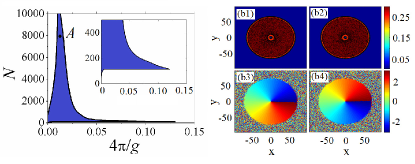
Figure 6: (a) The stability area of HV modes, defined as per Eq. (30), in the plane of $(N,4\pi/g)$, in the model based on Eq. (1) with $L_{3}=0$. The indigo (medium gray) area is bounded by the lower and upper limit values, see Eq. (32), with nearly constant values of $N_{\mathrm{th}}^{\mathrm{(low)}}$, as seen in the inset. (b) Density and phase plots showing opposite vorticities of the two components of a stable HV mode, with $(N,4\pi/g)=(8000,0.11)$, which corresponds to point A in (a), as a result of the evolution simulated up to $t=10000$.

Simulations of the perturbed evolution of unstable HV states (not shown here in detail) demonstrate that vortex cores in their two components split and start drifting in different directions, being eventually expelled from the pattern. The final outcome is, in many cases, merger of the unstable HV state into a zero-vorticity soliton.

IV Physical estimates

Translating the scaled units into physical ones (in particular, as per Refs. Cabrera2017 ; Cabrera2 ), we conclude that the predicted vortex modes may have radial size $R$ up to $\lesssim 30$ $\mathrm{\mu}$m and transverse thickness $\lesssim 1$ $\mathrm{\mu}$m, containing $10^{4}-10^{5}$ atoms, with density $\sim 10^{14}$ cm^-3. The radial size may be essentially larger than observed in recent experiments for zero-vorticity oblate droplets Cabrera2017 ; Cabrera2 , as they tend to swell under the action of the embedded vorticity, as seen in Figs. 2(a,b) and 2.

To address the role of the three-body loss, we note that the loss rate in physical units for ³⁹K is $\simeq 10^{-27}$ cm⁶/s Shlyap . With the above-mentioned typical densities, $n\sim 10^{14}$ cm³, this implies the decay time $t_{\mathrm{decay}}\simeq 10\left(Kn^{2}\right)^{-1}\sim 1$ s, which is $t\sim 1000$ in terms of our scaled notation. Then, the respective estimate for the scaled loss coefficient is $L_{3}\sim 0.01$. Figure 3(d) displays the simulated evolution, in the framework of Eq. (3), of the density pattern for an originally stable vortex QD with $(S,L_{3})=(1,0.01)$ and initial norm $N_{0}=1000$. The loss gives rise to shrinkage of the QD, which keeps the flat-top shape, with the fixed density, $|\psi|^{2}\approx n_{\mathrm{p}}^{\mathrm{(TF)}}$, as per Eq. (13), until the slowly decaying norm drops below the stability threshold, $N_{\mathrm{th}}$ [see Fig.. 3(a2)], causing quick spitting of the vortex mode. Similarly, sudden splitting into $S+1$ fragments, on the experimentally relevant time scale, is caused by the loss-induced evolution of originally stable droplets with $S>1$, provided that $N_{0}$ is not too large.

The loss-induced shrinkage of the flat-top droplets can be easily predicted analytically. As follows from the full equation (3), the total norm decays in time as

$$\frac{dN}{dt}=\frac{L_{3}}{2}\int\int|\psi|^{6}dxdy.$$ (33)

Further, it follows from here that external radius $R$ of the flat-top QD with inner density $n_{\mathrm{p}}$ given by Eq. (13), which is related to $N$ according to Eq. (23), shrinks in the course of the loss-induced evolution as

$$R(t)=R_{0}\exp\left(-\frac{{L_{3}}t}{4e}\right),$$ (34)

where $R_{0}$ is the initial radius, the corresponding decay law of the norm being

$$N(t)=\left(\frac{\pi}{\sqrt{e}}\right)R_{0}^{2}\exp\left(-\frac{{L_{3}}t}{2e}\right).$$ (35)

Predictions produced by Eqs. (34) and (35) are well corroborated by the numerical simulations.

The present analysis is performed in the zero-temperature limit (the condensation point in the experimentally relevant setting is $T_{\mathrm{BEC}}\simeq 150$ nK K-39 ). Finite-$T$ effects for zero-vorticity droplets were recently studied in Ref. T , by means of the Hartree-Fock-Bogoliubov-Popov Nick theory, with a conclusion that the thermal component forms a halo around the droplets. A similar prediction is expected for the vortex QDs, with some density of thermal atoms to be found in the droplet’s inner hole too. Detailed studies of the finite-$T$ setting should be a subject for a separate work.

V Interactions between quantum droplets and dynamics of elliptically deformed ones

Collisions between effectively one-dimensional QDs were recently analyzed in Ref. Grisha , where both quasi-elastic interactions and strongly inelastic outcomes, in the form of merger of colliding QDs, were reported. These results suggest to simulate collisions in the 2D setting too. Here, we aim to briefly consider this issue, while a detailed analysis will be a subject of a separate work.

Simulations, performed in the framework of Eq. (3) with ${L_{3}=0}$, demonstrate that the interaction between initially separated fundamental ($S=0$) QDs with zero phase difference leads, in the lossless model, to their merger into a single prolate droplet (which is a natural outcome for the fluid phase), that performs strong oscillations of eccentricity, as shown in Fig. 7(a1)-(a4). This excited mode resembles eccentricity oscillations performed by elliptically deformed circular kinks in the 2D sine-Gordon model Denmark .

Another option is the merger of two fundamental QDs, with opposite kicks initially applied to them in the transverse ($y$) direction (in other words, with torque applied to the QD pair), as shown in Fig. 7(b1)-(b4). This pair merges into a rotating prolate droplet. A different dynamical regime revealed by the simulations is rotation of an oval-shaped vortex with embedded vorticity $S=\pm 1$, see Fig. 7(c1)-(c4). The sign of embedded $S=+1$ or $-1$ correlates with the counter-clockwise or clockwise direction of the rotation. The consideration of these rotational regimes is suggested by recent studies of spinning helium nanodroplets Science ; PRB .

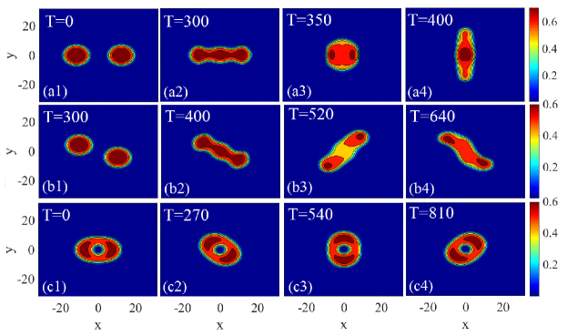
Figure 7: (a1)-(a4) Merger of two zero-vorticity QDs into a single droplet with strongly oscillating eccentricity, initiated by $\psi(\mathbf{r},t=0)=\phi(x-x_{0},y)+\phi(x+x_{0},y)$, with $x_{0}=12$ and norm $N=100$ of each QD. (b1)-(b4) Merger of two transversely kicked zero-vorticity QDs, with $S=0$, into a rotating elongated droplet, initiated by $\psi(\mathbf{r},t=0)=\phi(x-x_{0},y)e^{-iky}+\phi(x+x_{0},y)e^{iky}$, with $x_{0}=12$, $N=100$, and kick $k=0.015$. (c1)-(c4) Steady rotation of an oval-shaped vortex QD with vorticity $S=1$ and $N=200$. These results are produced by simulations of Eq. (3) with $L_{3}=0$.

Collisions between moving QDs were investigated too. The conclusions are similar to what is known about other nonintegrable models Spain ; BenLi , including the above-mentioned model for one-dimensional QDs Grisha : fast moving QDs pass through each other quasi-elastically, while slowly moving ones collide inelastically (not shown here). In particular, slowly colliding QDs with $S=0$ merge into a single droplet, while slowly colliding vortices suffer destruction.

VI Conclusion

The objective of this work is to investigate possibilities for the creation of effectively two-dimensional self-trapped QDs (quantum droplets) in the model based on nonlinearly coupled GPEs (Gross-Pitaevskii equations) for the binary BEC, with self-repulsion in each component and dominating attraction between them, the stabilization against the collapse being provided by the LHY (Lee-Huang-Yang) effect. As recently demonstrated, the nonlinearity in such an effective two-dimensional system takes the form of cubic terms multiplied by the additional logarithmic factor. We have constructed families of two-component QDs, with equal vorticities $S$, or opposite ones $\pm S$, embedded in each component, the latter species being called the HV (hidden-vorticity) mode. While the entire family with $S=0$ is stable, an essential finding is the stability region for the modes with the explicit vorticity (identical in both components), $1\leq S\leq 5$ (while the recent consideration of the vortex QDs in the 3D model reveals their stability solely for $S=1$ and $2$ Leticia ). All the modes with $S\geq 6$ are unstable in the region of norms, $N$, which are accessible for the analysis. Both the existence and stability boundaries for the vortex QDs have been identified, respectively, as $N_{\max}(S)$ and $N_{\mathrm{th}}(S)$. The steep growth of the latter value, $N_{\mathrm{th}}(S)\sim S^{4}$, and a still steeper scaling, $N_{\mathrm{th}}(S)\sim S^{6}$, predicted for three-dimensional QDs, has been explained analytically, considering the energy balance between the vortex mode and a set of fragments which may be produced by its splitting. At the stability boundary, the modes with $S=1,2,3$ seem as usual solitons with embedded vorticities, but deeper into the stability area, all vortex QDs develop a flat-top shape. While this feature may look similar to that known in models with competing self-focusing and defocusing nonlinear terms (e.g., the cubic-quintic NLS equation in two dimensions), the present system is essentially different, as it contains the single nonlinear term, $\sim|\psi|^{2}\psi\ln\left(|\psi|^{2}\right)$, as mentioned above.

It was demonstrated here too that pivots of all modes with multiple vorticities, $S\geq 2$, are subject to the structural instability, in the sense that specially selected small perturbations may split the single pivot into sets of $S$ or $S+2$ ones representing unitary vortices. However, the structural instability remains virtually invisible, as it occurs in the broad central “hole” of the multiple-$S$ vortex, where values of the fields are extremely small, and it does not cause any dynamical instability of the states with $S\geq 2$.

The nearly-constant value of the density in the flat-top area, and radius $r_{\min}$ of the central “hole” of the vortex mode (which is asymptotically independent of $S$) have been identified in the approximate analytical form, $r_{\min}$ being found by means of the Thomas-Fermi approximation. The role of the three-body loss, which may be an essential factor in the real experiment, was explored too, showing that it does not preclude the possibility of the creation and observation of stable vortex droplets (ones with relatively low initial norms may suddenly split under the action of the loss). The existence and stability boundaries for the QDs with all values of the explicit vorticity do not depend on the value of the coupling constant, $g$, of the GPE system. A possible stability region is also identified for HV modes, with vorticities $+1$ and $-1$ in its two components. Unlike the QDs with the explicit vorticity, stability of the HV states strongly depends on $g$, all states with $S_{+}=-S_{-}\geq 2$ being unstable. More complex robust dynamical modes were constructed and briefly considered too, viz., elliptically deformed QDs, with $S=0$ and $S=1$, which exhibit, severally, either strong eccentricity oscillations or steady rotation.

These results may find realizations in the ongoing experiments with QDs, some of which actually address nearly-2D configurations Cabrera2017 ; Cabrera2 . This possibility is quite important as, thus far, no stable bright vortex solitons have been created experimentally in free space or in any uniform physical medium. The vorticity may be imparted to the QD by a laser beam carrying an orbital optical momentum impart . The necessary condition for that is that the droplet’s size must be essentially larger than the wavelength of light, which definitely holds in the present setting.

In addition to the vortex states studied in this work, it may be relevant to address excited 2D states with a more complex radial structure. It may be also interesting to extend the systematic analysis to asymmetric two-component systems, with unequal scattering lengths accounting for the self-repulsion in the two components, and/or with unequal atomic masses (heteronuclear mixtures preprint ), as well as with unequal numbers of atoms in the two components. In particular, at finite temperature, the imbalance may imitate a controllable thermal bath Cabrera2 .

- (1) L. P. Pitaevskii and S. Stringari, Bose-Einstein Condensation (Oxford University Press: Oxford, 2003).
- (2) C. J. Pethick and H. Smith, Bose–Einstein Condensation in Dilute Gases (Cambridge University Press: Cambridge, 2008).
- (3) B. A. Malomed, D. Mihalache, F. Wise, and L. Torner, Spatiotemporal optical solitons, J. Optics B: Quant. Semicl. Opt. 7, R53-R72 (2005);Viewpoint: On multidimensional solitons and their legacy in contemporary Atomic, Molecular and Optical physics, J. Phys. B: At. Mol. Opt. Phys. 49, 170502 (2016).
- (4) L. Bergé, Wave collapse in physics: principles and applications to light and plasma waves, Phys. Rep. 303, 259-370 (1998).
- (5) G. Fibich, The Nonlinear Schrödinger Equation: Singular Solutions and Optical Collapse (Springer: Heidelberg, 2015).
- (6) B. A. Malomed, Multidimensional solitons: Well-established results and novel findings, Eur. Phys. J. Special Topics 225, 2507-2532 (2016).
- (7) M. Quiroga-Teixeiro and H. Michinel, Stable azimuthal stationary state in quintic nonlinear media, J. Opt. Soc. Am. B 14, 2004-2009 (1997).
- (8) R. L. Pego and H. A. Warchall, Spectrally stable encapsulated vortices for nonlinear Schrödinger equations, J. Nonlinear Sci. 12, 347-394 (2002).
- (9) T. A. Davydova and A. I. Yakimenko, Stable multicharged localized optical vortices in cubic-quintic nonlinear media, J. Opt. A: Pure Appl. Opt. 6, S197-S201 (2004).
- (10) D. Mihalache, D. Mazilu, L.-C. Crasovan, I. Towers, A. V. Buryak, B. A. Malomed, L. Torner, J. P. Torres, and F. Lederer, Stable spinning optical solitons in three dimensions, Phys. Rev. Lett. 88, 073902 (2002).
- (11) E. L. Falcão-Filho, and C. B. de Araújo, G. Boudebs, H. Leblond, and V. Skarka, Robust two-dimensional spatial solitons in liquid carbon disulfide, Phys. Rev. Lett. 110, 013901 (2013).
- (12) A. S. Reyna, G. Boudebs, B. A. Malomed, and C. B. de Araújo, Robust self-trapping of vortex beams in a saturable optical medium, Phys. Rev. A 93, 013840 (2016).
- (13) J. Qin, G. Dong, and B. A. Malomed, Stable giant vortex annuli in microwave-coupled atomic condensates, Phys. Rev. A 94, 053611 (2016).
- (14) H. Sakaguchi, B. Li, and B. A. Malomed, Creation of two-dimensional composite solitons in spin-orbit-coupled self-attractive Bose-Einstein condensates in free space, Phys. Rev. E 89, 032920 (2014).
- (15) L. Salasnich, W. B. Cardoso, and B. A. Malomed, Localized modes in quasi-two-dimensional Bose-Einstein condensates with spin-orbit and Rabi couplings, Phys. Rev. A 90, 033629 (2014).
- (16) Y. Li, Z. Luo, Y. Liu, Z. Chen, C. Huang, S. Fu, H. Tan, and B. A. Malomed, Two-dimensional solitons and quantum droplets supported by competing self- and cross-interactions in spin-orbit-coupled condensates, New. J. Phys. 19, 113043 (2017).
- (17) Y.-C. Zhang, Z.-W. Zhou, B. A. Malomed, and H. Pu, Stable solitons in three dimensional free space without the ground state: Self-trapped Bose-Einstein condensates with spin-orbit coupling, Phys. Rev. Lett. 115, 253902 (2015).
- (18) S. Gautam and S. K. Adhikari, Three-dimensional vortex-bright solitons in a spin-orbit-coupled spin-1 condensate, Phys. Rev. A 97, 013629 (2018).
- (19) F. Eilenberger, K. Prater, S. Minardi, R. Geiss, U. Röpke, J. Kobelke, K. Schuster, H. Bartelt, S. Nolte, A. Tünnermann, and T. Pertsch, Observation of discrete, vortex light bullets, Phys. Rev. X 3, 041031 (2013).
- (20) D. S. Petrov, Quantum Mechanical Stabilization of a collapsing Bose-Bose mixture, Phys. Rev. Lett. 115, 155302 (2015).
- (21) D. S. Petrov and G. E. Astrakharchik, Ultradilute Low-Dimensional Liquids, Phys. Rev. Lett 117, 100401 (2016).
- (22) T. D. Lee, K. Huang, and C. N. Yang, Eigenvalues and eigenfunctions of a Bose system of hard spheres and its low-temperature properties, Phys. Rev. 106, 1135 (1957).
- (23) Y. Sekino and Y. Nishida, Quantum droplet of one-dimensional bosons with a three-body attraction, Phys. Rev. A 97, 011602(R) (2018).
- (24) K. E. Strecker, G. B. Partridge, A. G. Truscott, and R. G. Hulet, Formation and propagation of matter-wave soliton trains, Nature 417, 150-153 (2002).
- (25) L. Khaykovich, F. Schreck, G. Ferrari, T. Bourdel, J. Cubizolles, L. D. Carr, Y. Castin, and C. Salomon, Formation of a matter-wave bright soliton, Science 296, 1290-1293 (2002).
- (26) K. E. Strecker, G. B. Partridge, A. G. Truscott, and R. G. Hulet, Bright matter wave solitons in Bose–Einstein condensates, New J. Phys. 5, 73 (2003).
- (27) S. L. Cornish, S. T. Thompson, and C. E. Wieman, Formation of bright matter-wave solitons during the collapse of attractive Bose-Einstein condensates, Phys. Rev. Lett. 96, 170401 (2006).
- (28) P. Medley, M. A. Minar, N. C. Cizek, D. Berryrieser, and M. A. Kasevich, Evaporative production of bright atomic solitons, Phys. Rev. Lett. 112, 060401 (2014).
- (29) P. J. Everitt, M. A. Sooriyabandara, G. D. McDonald, K. S. Hardman, C. Quinlivan, P. Manju, P. Wigley, J. E. Debs, J. D. Close, C. C. N. Kuhn, and N. P. Robins, Observation of breathers in an attractive Bose gas, arXiv:1509.06844
- (30) S. Lepoutre, L. Fouché, A. Boissé, G. Berthet, G. Salomon, A. Aspect, and T. Bourdel, Production of strongly bound 39K bright solitons, Phys. Rev. A 94, 053626 (2016).
- (31) A. Cappellaro, T. Macrí, G. F. Bertacco, and L. Salasnich, Equation of state and self-bound droplet in Rabi-coupled Bose mixtures, Sci. Rep. 7, 13358 (2017).
- (32) C. R. Cabrera, L. Tanzi, J. Sanz, B. Naylor, P. Thomas, P. Cheiney, L. Tarruell, Quantum liquid droplets in a mixture of Bose-Einstein condensates, Science 359, 301-304 (2018).
- (33) I. Ferrier-Barbut and T. Pfau, Quantum liquids get thin, Science 359, 274-275 (2018).
- (34) P. Cheiney, C. R. Cabrera, J. Sanz, B. Naylor, L. Tanzi, and L. Tarruell, Bright soliton to quantum droplet transition in a mixture of Bose-Einstein condensates, Phys. Rev. Lett. 120, 135301 (2018).
- (35) G. Semeghini, G. Ferioli, L. Masi, C. Mazzinghi, L. Wolswijk, F. Minardi, M. Modugno, G. Modugno, M. Inguscio, and M. Fattori, Self-bound quantum droplets in atomic mixtures, Phys. Rev. Lett. 120, 235301 (2018).
- (36) C. D’Errico, M. Zaccanti, M. Fattori, G. Roati, M. Inguscio, G. Modugno, and A. Simoni, Feshbach resonances in ultracold 39K, New J. Phys. 9, 223 (2007).
- (37) M. Lysebo and L. Veseth, Feshbach resonances and transition rates for cold homonuclear collisions between 39K and 41K atoms, Phys. Rev. A 81, 032702 (2010).
- (38) I. Ferrier-Barbut, H. Kadau, M. Schmitt, M. Wenzel, and T. Pfau, Observation of quantum droplets in a strongly dipolar Bose gas, Phys. Rev. Lett. 116, 215301 (2016).
- (39) M. Schmitt, M. Wenzel, F. Böttcher, I. Ferrier-Barbut, and T. Pfau, Self-bound droplets of a dilute magnetic quantum liquid, Nature 539, 259-262 (2016).
- (40) L. Chomaz, S. Baier, D. Petter, M. J. Mark, F. Wächtler, L. Santos, and F. Ferlaino, Quantum-fluctuation-driven crossover from a dilute Bose-Einstein condensate to a macrodroplet in a dipolar quantum fluid, Phys. Rev. X 6, 041039 (2016).
- (41) A. R. P. Lima, and A. Pelster, Quantum fluctuations in dipolar Bose gases, Phys. Rev. A 84, 041604(R) (2011).
- (42) H. Saito, Path-integral Monte Carlo study on a droplet of a dipolar Bose-Einstein condensate stabilized by quantum fluctuation, J. Phys. Soc. Jpn. 85, 053001 (2016).
- (43) K.-T. Xi and H. Saito, Droplet formation in a Bose-Einstein condensate with strong dipole-dipole interaction, Phys. Rev. A 93, 011604(R) (2016).
- (44) R. N. Bisset, R. M. Wilson, D. Baillie, and P. B. Blakie, Ground-state phase diagram of a dipolar condensate with quantum fluctuations, Phys. Rev. A 94, 033619 (2016).
- (45) F. Wächtler and L. Santos, Quantum filaments in dipolar Bose-Einstein condensate, Phys. Rev. A 93, 061603(R) (2016).
- (46) V. Pastukhov, Beyond mean-field properties of binary dipolar Bose mixtures at low temperatures, Phys. Rev. A 95, 023614 (2017)
- (47) F. Cinti and M. Boninsegni, Classical and quantum filaments in the ground state of trapped dipolar Bose gases, Phys. Rev. A 96, 013627 (2017).
- (48) D. Edler, C. Mishra, F. Wächtler, R. Nath, S. Sinha, and L. Santos, Quantum fluctuations in quasi-one-dimensional dipolar Bose-Einstein condensates, Phys. Rev. Lett. 119, 050403 (2017).
- (49) S. K. Adhikari, Statics and dynamics of a self-bound dipolar matter-wave droplet, Laser Phys. Lett. 14, 025501 (2017).
- (50) A. Cidrim, F. E. A. dos Santos, E. A. L. Henn, and T. Macrí, Vortices in self-bound dipolar droplets, Phys. Rev. A 98, 023618 (2018).
- (51) Y. V. Kartashov, B. A. Malomed, L. Tarruell, and L. Torner, Three-dimensional droplets of swirling superfluids, Phys. Rev. A 98, 013612 (2018).
- (52) W. Zheng, Z. Yu, X. Cui, and H. Zhai, Properties of Bose gases with the Raman-induced spin-orbit coupling, J. Phys. B: At. Mol. Opt. Phys. 46, 134007 (2013).
- (53) M. Brtka, A. Gammal, and B. A. Malomed, Hidden vorticity in binary Bose-Einstein condensates, Phys. Rev. A 82, 053610 (2010).
- (54) D. L. Feder, M. S. Pindzola, L. A. Collins, B. I. Schneider, and C. W. Clark, Dark-soliton states of Bose-Einstein condensates in anisotropic traps, Phys. Rev. A 62, 053606 (2000).
- (55) W. Z. Bao and Q. Du, Computing the ground state solution of Bose-Einstein condensates by a normalized gradient flow, SIAM J. Scientific Computing 25, 1674-1697 (2004).
- (56) D. Mihalache, D. Mazilu, B. A. Malomed, and F. Lederer, Vortex stability in nearly-two-dimensional Bose-Einstein condensates with attraction, Phys. Rev. A 73, 043615 (2006).
- (57) M. Vakhitov and A. Kolokolov, Stationary solutions of the wave equation in a medium with nonlinearity saturation, Radiophys. Quantum Electron. 16, 783-789 (1973).
- (58) Kh. I. Pushkarov, D. I. Pushkarov, and I. V. Tomov, Self-action of light beams in nonlinear media: soliton solutions, Opt. Quantum Electron. 11, 471-478 (1979).
- (59) S. Cowan, R. H. Enns, S. S. Rangnekar, and S. S. Sanghera, Quasi-soliton and other behavior of the nonlinear cubic-quintic Schrödinger equation, Can. J. Phys. 64, 311-315 (1986).
- (60) G. E. Astrakharchik and B. A. Malomed, Dynamics of one-dimensional quantum droplets, Phys. Rev. A 98, 013631 (2018).
- (61) A. Cappellaro, T. Macrì, and L. Salasnich1, Collective modes across the soliton-droplet crossover in binary Bose mixtures, Phys. Rev. A 97, 053623 (2018).
- (62) X. Cui, Spin-orbit-coupling-induced quantum droplet in ultracold Bose-Fermi mixtures, Phys. Rev. A 98, 023630 (2018).
- (63) V. Cikojević, K. Dželalija, P. Stipanović, and L. Vranješ Markić, Ultradilute quantum liquid drops, Phys. Rev. B 97, 140502(R) (2018).
- (64) C. Staudinger, F. Mazzanti, and R. E. Zillich, Self-bound Bose mixtures, Phys. Rev. A 98, 023633 (2018).
- (65) E. Chiquillo, Equation of state of the one- and three-dimensional Bose-Bose gases, Phys. Rev. A 97, 063605 (2018).
- (66) A. L. Fetter, Rotating trapped Bose-Einstein condensates, Rev. Mod. Phys. 81, 647-691 (2009).
- (67) Y. Kagan, B. V. Svistunov, and G. V. Shlyapnikov, Effect of Bose condensation on inelastic processes in gases, JETP Lett. 42, 209-212 (1985).
- (68) A. Boudjemâa, Quantum dilute droplets of dipolar bosons at finite temperature, Ann. Phys. (N.Y.) 381, 69-79 (2017).
- (69) Quantum Gases: Finite Temperature and Non-Equilibrium Dynamics, ed. by N. Proukakis, S. Gardiner, M. Davis, and M. Szymańska (Imperial College Press: London, 2013).
- (70) G. Modugno, G. Ferrari, G. Roati, R. J. Brecha, A. Simoni, and M. Inguscio, Bose-Einstein condensation of potassium atoms by sympathetic cooling, Science 294, 1320-1322 (2001).
- (71) P. L. Christiansen, N. Grønbech-Jensen, P. S. Lomdahl, and B. A. Malomed, Oscillations of eccentric pulsons, Physica Scripta 55, 131-134 (1997).
- (72) L. F. Gomez, K. R. Ferguson, J. P. Cryan, C. Bacellar, R. M. P. Tanyag, C. Jones, S. Schorb, D. Anielski, A. Belkacem, C. Bernando, R. Boll, J. Bozek, S. Carron, G. Chen, T. Delmas, L. Englert, S. W. Epp, B. Erk, L. Foucar, R. Hartmann, A. Hexemer, M. Huth, J. Kwok, S. R. Leone, J. H. S. Ma, F. R. N. C. Maia, E. Malmerberg, S. Marchesini, D. M. Neumark, B. Poon, J. Prell, D. Rolles, B. Rudek, A. Rudenko, M. Seifrid, K. R. Siefermann, F. P. Sturm, M. Swiggers, J. Ullrich, F. Weise, P. Zwart, C. Bostedt, O. Gessner, and A. F. Vilesov, Shapes and vorticities of superfluid helium nanodroplets, Science 345, 906-909 (2014).
- (73) F. Ancilotto, M. Barranco, and M. Pi, Spinning superfluid 4 He nanodroplets, Phys. Rev. B 97, 184515 (2018).
- (74) M. F. Andersen, C. Ryu, P. Cladé, V. Natarajan, A. Vaziri, K. Helmerson, and W. D. Phillips, Quantized rotation of atoms from photons with orbital angular momentum, Phys. Rev. Lett. 97, 170406 (2006); R. Pugatch, M. Shuker, O. Firstenberg, A. Ron, and N. Davidson, Topological stability of stored optical vortices ibid. 98, 203601 (2007).
- (75) F. Ancilotto, M. Barranco, M. Guilleumas, and M. Pi, Self-bound ultra dilute Bose mixtures within local density approximation, arXiv:1808.09197.