Multivariate Specification Tests Based on a Dynamic Rosenblatt Transform

Abstract

This paper considers parametric model adequacy tests for nonlinear multivariate dynamic models. It is shown that commonly used Kolmogorov-type tests do not take into account cross-sectional nor time-dependence structure, and a test, based on multi-parameter empirical processes, is proposed that overcomes these problems. The tests are applied to a nonlinear LSTAR-type model of joint movements of UK output growth and interest rate spreads. A simulation experiment illustrates the properties of the tests in finite samples. Asymptotic properties of the test statistics under the null of correct specification and under the local alternative, and justification of a parametric bootstrap to obtain critical values, are provided.

Keywords: Diagnostic test, joint distribution, multivariate modeling, Rosenblatt transform, LSTAR model.

JEL classification: C12, C22, C52.

1 Introduction

Robust nonparametric methods are hard to implement in a multidimensional case, and parametric modeling is often called for. For example, linear and nonlinear VAR models with Gaussian innovations are often used in macroeconometrics, while multivariate volatilities, which can be described by different types of multivariate GARCH (MGARCH) or copula-based models, are popular in financial econometrics. The use of a misspecified parametric model may result in misleading conclusions, in particular, biased estimates of monetary policy effects and underestimation of the risk in financial models. Thus it is crucial to develop specification testing procedures for these models. In a multidimensional context, it is important to know not only the time structure of the random vectors but also the dependence between contemporaneous variables, and this dependence should be used, for example, for portfolio diversification. Hence, we should be able to test for the correct specification of the joint multivariate distribution conditional on past information.

There is a huge literature on testing multivariate normality, see Mecklin and Mundform (2004). For testing a general type of distribution in a dynamic setup, a dynamic version of the Rosenblatt Transform (cf. Rosenblatt 1952), which is also a type of a Probability Integral Transform, PIT, allows us to approach all kinds of distributions in a unified manner. The idea is that, given the true conditional distribution, one can transform the data to independent and identically distributed (i.i.d.) uniform random variables and possibly further to normal i.i.d. Then, instead of testing the shape of the initial distribution, the uniformness and independence of the transformed data can be evaluated with histograms and correlograms, as suggested by Diebold et al. (1999) and Clements and Smith (2002) for multivariate density forecast evaluation. In practice, however, the distribution is known only up to parameters; therefore the method of Diebold et al. (1999) can not be applied. The reason is that, when estimates are plugged in, the (dynamic) Rosenblatt Transform delivers only approximately i.i.d. uniforms; moreover, the asymptotic distribution may change, and even become model and case dependent, see Durbin (1973). Ignoring parameter uncertainty introduces severe size distortions in such tests, as documented in simulations by Kalliovirta and Saikkonen (2010). The problem usually is solved by either transforming the statistics of interest to make them convergent to a known distribution (Khmaladze 1981, Wooldridge 1990, Delgado and Stute 2008, and many others) or by approximating critical values by the parametric bootstrap (Andrews 1997). For nonparametric testing of multivariate GARCH models, Bai and Chen (2008) developed a Kolmogorov-type testing procedure based on the dynamic Rosenblatt Transform. They applied a Khmaladze (1991) martingale transformation (K-transformation) to the empirical process to obtain a limiting distribution of statistics. However, in a univariate setup, Corradi and Swanson (2006) noted that Kolmogorov-type tests, based on a one-parameter empirical process, may not distinguish some important alternatives to the conditional distribution. In an i.i.d. setup with conditioning on covariates, Delgado and Stute (2008) proposed a consistent test using a two-parameter empirical process coupled with a Khmaladze martingale transformation. In a time series setup, where a Kolmogorov-type test does not capture misspecification in the dynamics, Kheifets (2015) proposed a test based on a multi-parameter empirical process and used a bootstrap to obtain critical values.

In this paper, we consider nonparametric testing of a multivariate distribution specification. We study the consequences of using a Kolmogorov-type test in this setup. We find that Kolmogorov-type tests result in missing both dynamic and cross-section dependence. To overcome this problem, we consider tests based on a multivariate empirical process, adapting the weak convergence results of Kheifets (2015) to a multivariate case. As well as a Kolmogorov test, our PIT-based procedure can test nonlinear models and capture deviations in marginal distribution. Besides that, our test includes two ingredients: a dynamic check (similar to Kheifets 2015) and a cross-section check. Thus our technique may be used not only for testing but also for investigating sources of misspecification. Our test complements the parametric tests of Kalliovirta and Saikkonen (2010) and Gonzalez-Rivera and Yoldas (2012). We avoid bandwidth selection, and our test statistics have a parametric rate of convergence, unlike the smoothing techniques of Hong and Li (2005), Li and Tkacz (2011), and Chen and Hong (2014), who use kernels to estimate the conditional distribution function and spectrum.

The contribution of the paper is the following: We develop the test and apply it to a model of UK growth and interest spreads and perform a set of Monte Carlo experiments to study the performance of the test in finite samples, where we observe results similar to Kolmogorov tests’ in some cases and improvement in others. We derive asymptotic properties of the test under the null and the local alternative, taking into account the parameter estimation effect, and justify the use of bootstrapped critical values.

The rest of the paper is organized as follows. Section 2 introduces specification test statistics, based on the dynamic Rosenblatt Transform. The empirical application is in Section 3. Monte Carlo experiments are shown in Section 4. Section 5 concludes. Asymptotic properties of the test are listed in the Appendix.

2 The Test Statistics

2.1 Our proposal

We now explain our methodology in detail. Suppose that a sequence of $d\times 1$ vectors $Y_{1},Y_{2},\ldots,Y_{T}$, where $Y_{t}=(Y_{t1},Y_{t2},\ldots,Y_{td})^{\prime},t=1,...,T,$ is given. Let $\Omega_{t}$ be the information set at time $t$ (not including $Y_{t}$), i.e., the $\sigma$-field of $\{Y_{t-1},Y_{t-2},\ldots\}$.

We consider a family of joint distributions $F_{t}(y|\Omega_{t},\theta)$, conditional on the past information, parameterized by $\theta\in\Theta$, where $\Theta\subseteq R^{L}$ is a finite dimensional parameter space. Apart from allowing the conditional (information) set $\Omega_{t}$ to change with time, we permit change in the functional form of the distribution using subscript $t$ in $F_{t}$. Our null hypothesis of correct specification is:

$H_{0}$ : The multivariate distribution of $Y_{t}$ conditional on $\Omega_{t}$ is in the parametric family $F_{t}(y|\Omega_{t},\theta)$ for some $\theta_{0}\in\Theta$.

Note that by specifying the multivariate conditional distribution, we specify many properties of the data simultaneously, such as multivariate and univariate marginal distributions, univariate conditional distributions, time and cross-section dependence, symmetry, all existing moments, kurtosis, etc. Many dynamic models can be written in the form of a conditional distribution. Examples include (non)linear vector autoregressive (VAR) and MGARCH models with i.i.d. parametric innovations, copula-based models with parametric marginals and possibly time-varying copula functions, and discretely sampled continuous-time models represented by a stochastic differential equation.

We now describe how to use PIT. In a simple univariate unconditional testing, we have that if $Y\sim F(\cdot)$, then $U=F(Y)$ is uniform, which is the base of the Kolmogorov test. More precisely, the null hypothesis of the Kolmogorov test is that $F(Y)$ is uniform. If we are interested in conditional distribution testing, which is the case when we have covariates or dynamics, we use the fact that if $Y_{t}|\Omega_{t}\sim F_{t}(\cdot|\Omega_{t})$, then $U_{t}=F(Y_{t}|\Omega_{t})$ is uniform and i.i.d. The distribution needs to be absolutely continuous. For a discrete distribution, one may use a different transform, see Kheifets and Velasco (2013, 2017).

In multivariate setup, $F(Y),$ which seems to be an obvious generalization of the PIT, is not generally uniform for a vector $Y\sim F(\cdot)$. $F(Y)$ is related to copula functions, which describe multivariate dependence without specifying marginals. The properties of $F(Y)$ were studied in Genest and Rivest (2001). In this paper we want to check the specification of the multivariate distribution; therefore, testing the specification of the copula function is not sufficient. For a multivariate PIT, we need to define the conditioning sets properly. Following Rosenblatt (1952) and Diebold et al. (1999), construct a long univariate series by stacking sequentially $Y_{t}$ to get a $n=Td$ long univariate series, which we denote

$$\{Z_{k}\}_{k=1}^{n}:=\{...,Y_{t1},Y_{t2},...,Y_{td},...\}_{t=1}^{T}.$$ (1)

In other words, $Z_{k}=Y_{t\ell}$ for $t=\lceil k/d\rceil$ and $\ell=k-td$, where $k=1,...,n$, $t=1,...,T$, $\ell=1,...,d$, and $\lceil x\rceil$ denotes the smallest integer not less than $x$. There are many ways to order and stack $Y_{t\ell}$; for example, $\{...,Y_{t2},Y_{t1},...,Y_{td},...\}$ is another possibility. Although the ordering determines the test statistics, in practice we are not able to test all possible orderings. In our Monte Carlo experiments, we study how the choice of a particular order affects the performance of the test. From the null multivariate conditional distributions $F_{t}(y|\Omega_{t},\theta_{0})$, we can obtain univariate conditional distributions $F_{Z_{k}}(z|\Omega_{k}^{Z},\theta_{0})$, where $\Omega_{k}^{Z}$ is a $\sigma$-field of $\{Z_{1},Z_{2},...,Z_{k-1}\}$. To do this, for each $t$, apply to the joint distribution $d$ times the factorization $F\left(y_{1},y_{2}\right)=F\left(y_{1}\right)F\left(y_{2}|y_{1}\right)$. Now apply $n$ times PIT

$$U_{k}=F_{Z_{k}}(Z_{k}|\Omega_{k}^{Z},\theta_{0}),$$

which are uniform and i.i.d. This is a dynamic analog of a multivariate Rosenblatt (1952) transform. Explicit formulas of such transforms for VAR models with possible MGARCH innovations can be found in Bai and Chen (2008) and Kalliovirta and Saikkonen (2010); for copula-based models see Patton (2013), see also A.2 for an example.

Under the null, $\{U_{k}\}_{k=1}^{n}$ are uniform and i.i.d. Diebold et al. (1999) use this fact for density forecast evaluation by looking at histograms and correlograms of $U_{t}$. In this paper, we use the ideas of Delgado and Stute (2008) and Kheifets (2015) to make a formal testing procedure for $H_{0}$ that requires us to check simultaneously uniformness and independence. For $k=2,...,n$, using pairwise independence and uniformness, we have

$$\Pr({U}_{k}\leq r_{1},{U}_{k-1}\leq r_{2})=r_{1}r_{2},$$

for $r\in{[0,1]}^{2},$ which motivates us to consider the following empirical processes

$${V}_{2T}(r)=\frac{1}{\sqrt{n-1}}\sum_{k=2}^{n}\left[I({U}_{k}\leq r_{1})I({U}_{k-1}\leq r_{2})-r_{1}r_{2}\right].$$ (2)

If we do not know $\theta_{0}$, we approximate $U_{k}$ with

$$\hat{U}_{k}=F_{Z_{k}}(Z_{k}|\Omega^{Z}_{k},{\hat{\theta}}),$$

where ${\hat{\theta}}$ is an estimator of $\theta_{0}$, so that

$$\hat{V}_{2T}(r)=\frac{1}{\sqrt{n-1}}\sum_{k=2}^{n}\left[I(\hat{U}_{k}\leq r_{1})I(\hat{U}_{k-1}\leq r_{2})-r_{1}r_{2}\right].$$ (3)

To obtain a test statistic, define

$$D_{2T}=\Gamma(\hat{V}_{2T}(r)),$$

for any continuous functional $\Gamma(\cdot)$ from $\ell^{\infty}([0,1]^{2})$, the set of uniformly bounded real functions on $[0,1]^{2}$, to $R$. In particular, we consider Cramer-von Mises (CvM) and Kolmogorov-Smirnov (KS) statistics

$$D_{2T}^{CvM}=\int_{[0,1]^{2}}\hat{V}_{2T}(r)^{2}dr\text{ and }D_{2T}^{KS}=\sup_{[0,1]^{2}}\left|\hat{V}_{2T}(r)\right|.$$ (4)

The choice of the measure is an interesting question in itself; it may make the test more powerful for some particular alternatives. Here we stick just to these two.

To check $p$-wise independence in a similar way to Delgado (1996), we can base test statistics on the $p$-parameter process

$${V}_{pT}(r)=\frac{1}{\sqrt{n-p}}\sum_{k=p}^{n}\left[\prod_{j=1}^{p}I({U}_{k-j+1}\leq r_{j})-r_{1}r_{2}\ldots r_{p}\right],$$

using norms on $[0,1]^{p},$ say,

$$D_{pT}^{CvM}=\int_{[0,1]^{p}}\hat{V}_{pT}(r)^{2}dr\text{ and }D_{pT}^{KS}=\sup_{[0,1]^{p}}\left|\hat{V}_{pT}(r)\right|.$$ (5)

The test based on the process with $p=1$ does not have power against many important alternatives, e.g., omitted autoregressive terms in mean or variance. Such alternatives are captured by tests with $p=2$. In the rest of the paper we consider such tests.

To test other than one-lag pairwise dependence, for $j=1,2,...$ define the process

$$\hat{V}_{2T,j}(r)=\frac{1}{\sqrt{n-j}}\sum_{k=j+1}^{n}\left[I(\hat{U}_{k}\leq r_{1})I(\hat{U}_{k\text{-}j}\leq r_{2})-r_{1}r_{2}\right],$$

with test statistics,

$$D_{2T,j}^{CvM}=\int_{[0,1]^{2}}\hat{V}_{2T,j}(r)^{2}dr\text{ and }D_{2T,j}^{KS}=\sup_{[0,1]^{2}}\left|\hat{V}_{2T,j}(r)\right|.$$ (6)

In order to provide some guidance for a practitioner, we propose the following interpretation of the test statistics above. For example, for linear bivariate model $D_{2T,1}$ controls cross-sectional dependence, while $D_{2T,2}$ controls dynamic specification. In DGP-A1, DGP-C5 and DGP-C6 in the Monte Carlo section below, cross-sectional dependence is misspecified. Such alternatives are captured by $D_{2T,1}$. In DGP-A3, the dynamics in the first variable is misspecified, hence $D_{2T,2}$ catches it. Marginal checks are included in both statistics, i.e., misspecification of the marginal distribution will result in high values for all test statistics. To test the null hypothesis against an unknown alternative, aggregate information from these statistics. Following the notation of Kheifets (2015), define for $k=1,...,n-1$ the test statistics

$$ADJ_{kT}=\sum_{j=1}^{k}D_{2T,j}^{CvM}\text{ and }MDJ_{kT}=\max_{j=1,...,k}D_{2T,j}^{KS},$$

and

$$ADJ_{kT}^{0}=D_{1T}^{CvM}+ADJ_{kT}\text{ and }MDJ_{kT}^{0}=\max\left(D_{1T}^{KS},MDJ_{kT}\right).$$

Test statistics $ADJ_{kT}$ and $MDJ_{kT}$ summarize the information from different lags, in the spirit of a Ljung-Box (1978) test, for which choosing small $k$ may miss higher order dependence, while choosing large $k$ reduces overall power. Test statistics $ADJ_{kT}^{0}$ and $MDJ_{kT}^{0}$ additionally take into account the marginal distribution of the data explicitly.

Since, under $H_{0}$, we know (up to the parameter value) the parametric conditional distribution, we apply a parametric bootstrap to mimic the $H_{0}$ distribution based on $F_{t}(\cdot|\cdot,\hat{\theta})$. This will require additional computational time; however, note that even in the case of asymptotic distribution free tests, bootstrap critical values may be preferred to asymptotic ones in terms of finite sample performance, see Kilian and Demiroglu (2000). We introduce the algorithm now.

1. Estimate the model with the original data $Y_{t}$, $t=1,2,...,T$ to get parameter estimator $\hat{\theta}$ and test statistic $\Gamma(\hat{V})$.

2. Simulate $Y_{t}^{\ast}$ with $F_{t}(\cdot|\Omega_{t}^{\ast},\hat{\theta})$ recursively for $t=1,2,...,T$, where $\Omega_{t}^{\ast}=(Y_{t-1}^{\ast},Y_{t-2}^{\ast},...)$.

3. Estimate the model with simulated data $Y_{t}^{\ast}$ to get $\theta^{\ast}$ and bootstrapped statistics $\Gamma(\hat{V}^{\ast})$.

4. Repeat 2-3 $B$ times, and compute the percentiles of the empirical distribution of the $B$ bootstrapped statistics.

5. Reject $H_{0}$ if $\Gamma(\hat{V})$ is greater than the $(1-\alpha)$ th percentile of the empirical distribution.

We recommend setting $B$ to at least $1000$, the number used in this paper. Bootstrapping critical values takes 15 minutes for the bivariate LSTAR model considered in Section 3, see A.4 for further computational details. For some bootstrap samples the estimation routine may fail. For example, when an explicit solution to a model exists, numerical methods may not be able to invert an ill-conditioned matrix. In case of highly nonlinear models, extremum estimation procedures may take a long time to converge or even to return an error. In these cases, $B$ should be larger so that the bias in the bootstrapped quantiles, which may appear after omitting those samples, is acceptable to a researcher.

Theoretical properties of the procedure developed in this paper rely on 1) the dynamic extension of the Rosenblatt transform and 2) the weak convergence result in Kheifets (2015). The latter proposes a specification test for univariate models based on multi-parameter empirical processes and studies the convergence of such processes, which allows us to justify the use of the bootstrapped critical values. These theoretical results can be employed for our needs because the Rosenblatt transforms are univariate (and uniformly and independently distributed under the null hypothesis). In order to do so, we need to verify high-level assumptions of Kheifets (2015) under the dynamic extension of the Rosenblatt transform, please see A.3 for details.

2.2 Comparison with Bai and Chen (2008) and related tests

Most of the tests for $H_{0}$ use some particular properties of the null distribution, such as skewness, kurtosis or correlation, whether of the initial data or of that of transformed variables (i.e., residuals, PITs or composition of PITs, and transforms to normal random variables). One exception is the test of Bai and Chen (2008), which is a nonsmooth omnibus-type test for multivariate GARCH models. In fact, they can test our $H_{0}$. Their test statistic is based on a combination of empirical processes

$${J}_{T,\ell}(r)=\frac{1}{\sqrt{T}}\sum_{t=1}^{T}\left[I({U}_{(t-1)d+\ell}\leq r)-r\right],$$

for $r\in[0,1]$, $\ell=1,\ldots,d$. In particular, they propose three combinations: taking the maximum, $\max_{\ell=1,\ldots,d}\sup_{r\in[0,1]}|{J}_{T,\ell}(r)|$, taking the sum, $\sum_{\ell=1,\ldots,d}\sup_{r_{\ell}\in[0,1]}|{J}_{T,\ell}(r_{\ell})|$, and pooling $\sup_{r\in[0,1]}|\frac{1}{\sqrt{d}}\sum_{\ell=1,\ldots,d}{J}_{T,\ell}(r)|$, corresponding to $D_{1T}^{KS}$ in our notation. They further apply a K-transformation to obtain the convergence to the supremum of a standard Brownian motion, even in the presence of parameter estimation. However, these types of processes miss the dynamic check in $U_{k}$, i.e., the critique raised by Corradi and Swanson (2006) for univariate tests applies in a multivariate case as well. The key element of our procedure is to use the test statistics based on the multivariate processes $D_{pT}$, $p>1$. In the next section, we compare the performance of the test statistics $D_{1T}$ and $D_{2T}$ using Monte Carlo simulations.

Another common strategy is to bootstrap CvM or KS statistics based on the following “row-wise” empirical process (e.g., Patton 2013, Section 4.1, but note a typo in the standardization, should be $\frac{1}{\sqrt{T}}$ instead of $\frac{1}{{T}}$)

$${S}_{pT}(r)=\frac{1}{\sqrt{T}}\sum_{t=1}^{T}\left[\prod_{\ell=1}^{d}I({U}_{(t-1)d+\ell}\leq r_{j})-r_{1}r_{2}\ldots r_{d}\right],$$

for $r\in[0,1]^{d}$. Unlike the tests based on $J_{T,\ell}$, tests based on this empirical process do take some dynamics in $U_{k}$ into account, but not all. In particular, independence is controlled within, but not between, the rows $U^{t}=({U}_{(t-1)d+1},{U}_{(t-1)d+2},\ldots,{U}_{(t-1)d+d})$. For instance, in a bivariate case, (cross-sectional) independence between $U_{2t-1}$ and $U_{2t}$, $t=1,\ldots,T$ is controlled, while (dynamic-cross) independence between $U_{2t}$ and $U_{2t+1}$ and (pure dynamic) independence between $U_{2t-1}$ and $U_{2t+1}$ and between $U_{2t}$ and $U_{2t+2}$ are not. The empirical process $V_{pT}$, suggested in our paper, overcomes these problems.

We calculate critical values using a parametric bootstrap. In a similar (although univariate) situation, Corradi and Swanson (2006) suggest the use of a block bootstrap, which delivers correct critical values under dynamic misspecification. Our approach is different in two respects. First, we do not require strict stationarity, while their block bootstrap approximation relies on it. Second, in our case dynamic misspecification is not allowed under the null and must be detected if present. For example, predictions of output growth and spreads considered in our empirical application are based on all available information. That is why the conditional set in our null hypothesis is $\Omega_{t}$ and not $Y_{t-1}$.

Bai and Chen (2008) apply K-transformation to obtain a distribution-free test. Extending these kinds of transformations to our case is non-trivial because the empirical processes are multivariate and the same variables enter different dimensions, introducing dependence among dimensions. A parametric bootstrap is an attractive alternative to such techniques because it requires repeated simulation and estimation of the null model, while implementing a K-transform requires one to derive analytically the transform for each model under consideration, which is not straightforward (see examples in Bai and Chen, 2008).

3 Empirical Application

We test a model for joint movement of output growth and the interest rate spread in the UK, plotted on Figure 1 and suggested by Anderson, Athanasopoulos, and Vahid (2007, AAV hereafter). Output growth ($Y_{t1}$) is calculated as $100$ $\times$ the difference of logarithms of seasonally adjusted real DGP, and the spread ($Y_{t2}$) is the difference between the interest rates on 10 Year Government Bonds and 3 Month Treasury Bills. The sample consists of $159$ quarterly time series observations, dating from 1960:3 to 1999:4 and available, together with the GAUSS programs, at the AAV accompanying webpage (http://qed.econ.queensu.ca/jae/2007-v22.1/anderson-athanasopoulos-vahid/).

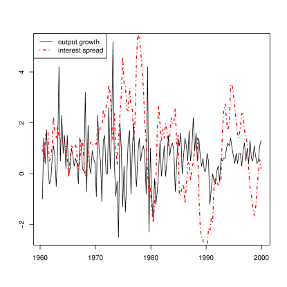
Figure 1: UK output growth and interest spread, quarterly data from 1960:3 to 1999:4

AAV suggested the following model for the conditional mean of $Y_{t}$, $\mu_{t}=\left(\mu_{t1},\mu_{t2}\right)^{\prime}$ as a function of unknown parameters $b=\left(b_{1},\ldots,b_{11}\right)^{\prime}$

$$\mu_{t1} = b_{1}+b_{2}Y_{t-2,1}+b_{3}Y_{t-3,2}+b_{4}Y_{t-1,2}+w_{t}\left(-b_{5}Y_{t-1,2}\right),$$

$$\mu_{t2} = b_{8}+b_{9}Y_{t-3,1}+b_{10}Y_{t-1,2}+b_{11}Y_{t-2,2},$$

$$\text{where }w_{t} = \left(1+\exp\left(-b_{6}(Y_{t-2,1}-b_{7})\right)\right)^{-1}.$$

The logistic smooth transition autoregressive specification for output growth incorporates different regimes and smooth transitions between them.

AAV estimated the model by ML and obtained predicted values by simulation, using (conditional) normality of errors. This motivates us to test the following null hypothesis

$$H_{0}:Y_{t}|\Omega_{t}\sim N(\mu_{t},\Sigma),\text{ where $\Sigma$ is independent of $\Omega_{t}$.}$$ (7)

Assuming (7), we obtain $\hat{b}=\left(0.35,0.21,0.15,0.32,-0.52,2.56,0.68,0.20,-0.14,1.14,-0.26\right)^{\prime}$ and $\Sigma=\left(0.95,-0.02;-0.02,0.45\right)$. AAV report only the estimate of $b$, not $\Sigma$. Our estimate of $b$ is close to theirs. Tests’ $p$-values are reported in Table 1. As in AAV, we detect no remaining serial correlation. However, the nonlinear procedure proposed in our paper suggests that the null hypothesis (7) can be rejected at the $1\%$ confidence level.

Table 1: $100$ $\times$ $p$-values of tests for the null hypothesis defined in Section 3 applied to the UK data. Both Cramer-von Mises and Kolmogorov-Smirnov norms are used. Tests based on the one-parameter process, the two-parameter process with 1st lag for cross sectional dependence, and the two-parameter process with 2d lag for time dependence, as well as Ljung-Box (Box et al., 1994) test statistics with $1$, $2$, $3$, $20$, and $25$ lags, are considered. Sample size is $T=156$.

		$D_{1}^{CvM}$	$D_{2,1}^{CvM}$	$D_{2,2}^{CvM}$	$D_{1}^{KS}$	$D_{2,1}^{KS}$	$D_{2,2}^{KS}$	$LBQ_{1}$	$LBQ_{2}$	$LBQ_{3}$	$LBQ_{20}$	$LBQ_{25}$
		$0.2$	$0.5$	$0.0$	$0.0$	$0.0$	$0.0$	$31.3$	$54.9$	$68.1$	$31.4$	$48.3$

Monte Carlo experiments conducted in the next section show that the empirical size of our tests is close to nominal. Simulations C2, C3, and C4 in the next section also suggest that alternative models with Student-$t$ distribution and the same dynamics as in (7) can hardly be captured by serial correlation checks, while our tests have power for sample size $T=100$.

4 Monte Carlo Experiments

We study the performance of our procedure under the null and alternative hypotheses using Monte Carlo experiments discussed in Giacomini, Politis and White (2013). We also show the rejection rates for parametric tests Ljung and Box (1978) and Jarque and Bera (1980) (for Part C). For comparison purposes, their distributions are obtained using bootstrap. We start with a simple linear null hypothesis and linear DGP, where model estimation is simple and estimators converge fast, allowing us to see the finite sample behavior of the proposed statistics; then we proceed to a nonlinear model motivated by our empirical example and calibrated to real data. All DGPs are listed in Table 2. The number of Monte Carlo repetitions is set to $1000$.

Table 2: The list of DGP used in Monte Carlo simulations

1. DGP-A1: $Y_{t}|\Omega_{t}\sim N\left(\left(0,0\right)^{\prime},\left(2,\alpha;\alpha,1\right)\right)$

2. DGP-A2: $Y_{t}|\Omega_{t}\sim t_{5}\left(\left(0,0\right)^{\prime},\left(2,\alpha;\alpha,1\right)\right)$

3. DGP-A3: time series with lag-$1$ dependence are normally distributed $Y_{t}|\Omega_{t}\sim N\left(A_{1}Y_{t-1},(1,0;0,1)\right)$, where $A_{1}=(\alpha,0;0,0)$.

4. DGP-B1: $Y_{t}|\Omega_{t}\sim N\left(\left(0,0\right)^{\prime},\left(1,0.5;0.5,1\right)\right)$,

5. DGP-B2: $Y_{t}|\Omega_{t}\sim N\left(\left(0,0\right)^{\prime},\left(1,0.5;0.5,2\right)\right)$,

6. DGP-B3: $Y_{t}|\Omega_{t}\sim N\left(\left(0,0\right)^{\prime},\left(2,0.5;0.5,1\right)\right)$,

7. DGP-B4: $Y_{t}|\Omega_{t}\sim t_{5}\left(\left(0,0\right)^{\prime},\left(1,0.5;0.5,1\right)\right)$,

8. DGP-B5: $Y_{t}|\Omega_{t}\sim t_{5}\left(\left(0,0\right)^{\prime},\left(1,0.5;0.5,2\right)\right)$,

9. DGP-B6: $Y_{t}|\Omega_{t}\sim t_{5}\left(\left(0,0\right)^{\prime},\left(2,0.5;0.5,1\right)\right)$,

10. DGP-C1: $Y_{t}$ is generated by the model considered in Section 3, with $b$ and $\Sigma$ equal to the estimate obtained therein.

11. DGP-C2: $Y_{t}$ as in DGP-C1, but with conditional distribution Student $t_{7}$ instead of normal.

12. DGP-C3: $Y_{t}$ as in DGP-C1, but with conditional distribution Student $t_{5}$ instead of normal.

13. DGP-C4: $Y_{t}$ as in DGP-C1, but with conditional distribution Student $t_{3}$ instead of normal.

14. DGP-C5: $Y_{t}$ as in DGP-C1, but with conditional mean for the output $\tilde{\mu}_{t1}=\mu_{t1}+0.5Y_{t-2,2}$.

15. DGP-C6: $Y_{t}$ as in DGP-C1, but with conditional mean for the output $\tilde{\mu}_{t1}=\mu_{t1}+0.9Y_{t-2,2}$.

4.1 Part A

In this subsection, we study the finite sample performance of the test statistics to test the null hypothesis that the series is identically multivariate normally distributed and is time and cross-section independent,

$$H_{0}:Y_{t}|\Omega_{t}\sim N(\mu,\Sigma),\text{ where $\mu,\Sigma$ are independent of $\Omega_{t},$ and $\Sigma$ is diagonal}.$$ (8)

We study this null hypothesis under three types of alternatives:

1. DGP-A1: series are cross-section dependent, normally distributed,

2. DGP-A2: series are cross-section dependent, $t_{5}$ distributed, and

3. DGP-A3: series are time dependent, normally distributed,

where in all cases the parameter $\alpha$ takes values $0,0.1,...,0.9.$ The value $\alpha=0$ generates data under the null in DGP-A1 and DGP-A3, so empirical power should be around nominal. Increasing $\alpha$ makes deviation from the null stronger, so the power should increase.

We study empirical power of the tests $D_{1}$, $D_{2,1}$ and $D_{2,2}$, defined in (5) and (6). In Figure 2(a), $5\%$ rejection rates of Cramer von Misses tests for DGP-A1 are plotted. We see that both $D_{1}$ and $D_{2,2}$ have near nominal $5\%$ power for all $\alpha$. Test $D_{2,1}$, on the contrary, is able to detect alternatives starting from small power at $\alpha=0.2$ and increasing up to almost $80\%$ for $\alpha=0.9$. In Figure 2(c), Cramer von Misses tests for DGP-A2 are plotted. All tests have at least $50\%$ rejection rates for all $\alpha$. In Figure 2(e), Cramer von Misses tests for DGP-A3 are plotted. We see that both $D_{1}$ and $D_{2,1}$ have near $5\%$ power for all $\alpha$. Test $D_{2,2}$, on the contrary, is able to detect alternatives starting from small power at $\alpha=0.2$ and increasing up to more than $90\%$ for $\alpha=0.9$. The picture does not change if we use a KS-norm.

In sum, we have observed that $D_{2,1}$ captures cross-sectional misspecification and $D_{2,2}$ is able to capture misspecification in dynamics, while $D_{1}$ detects neither. All three tests perform equally well when the marginal distribution is misspecified.

(a) CvM against DGP-A1

(b) KS against DGP-A1

(c) CvM against DGP-A2

(d) KS against DGP-A2

(e) CvM against DGP-A3

(f) KS against DGP-A3

Figure 2: Rejection proportions of tests for Normal time and cross-section independent null hypothesis (8). Panel (a) shows the performance of the Cramer-von Mises tests for cross-section dependent normal DGP-A1. Panel (b) shows the performance of the Kolmogorov-Smirnov test for the same GDP. Panels (c) and (d) show the performance of the corresponding tests for Student-t with 5 degrees of freedom $t_{5}$ DGP-A2. Panels (e) and (f) show the performance of the corresponding tests for cross-section independent normal VAR(1) DGP-A3. Tests based on one-parameter process (circle markers), two-parameter process with the first lag for cross sectional dependence (triangular markers) and two-parameter process with the second lag for time dependence (cross markers) are considered. Rejections at $5\%$ are plotted with a dotted line. Sample sizes are $T=100$.

4.2 Part B

We study the finite sample performance of the test statistics to test the null hypothesis that the series is multivariate normal,

$$H_{0}:Y_{t}|\Omega_{t}\sim N(\mu,\Sigma),\quad\text{where}\ \mu\ \text{and}\ \Sigma\ \text{are independent of}\ \Omega_{t}.$$ (9)

Note that now $\Sigma$ need not be diagonal, so we allow cross-sectional dependence but not temporal. DGP-B1 to DGP-B3 generate data under the parametric family null hypothesis (9) and deliver the empirical size of the test. DGP-B4 to DGP-B6 simulate data under the $t_{5}$ distribution, a popular alternative to normality that accounts for fat tails, and deliver the empirical power of the test. DGP-B1 and DGP-B4 were considered also in Bai and Chen (2008). DGP-B2, DGP-B3, DGP-B5, and DGP-B6 are taken to assess the influence of the order choice in (1). We consider the cases both when the distribution is symmetric with respect to the coordinates and when it is not. When the distribution is not symmetric, exchanging the coordinates is equivalent to changing the order in (1), and we want to know if, and how, it affects the performance of the test. In the normal case, this symmetry is reflected by the restriction on the covariance matrix $\Sigma_{t11}=\Sigma_{t22}$, case DGP-B1,4.

We study the performance of tests $D_{1}$, $D_{2,1}$, and $D_{2,2}$, as defined in (5) and (6) and Ljung-Box (Box et al., 1994) test statistics with $1$, $2$, $3$, $20$, and $25$ lags. In Table 3, sample sizes are $T=100$. DGP-B1 to DGP-B3 are contained in the null hypothesis and deliver empirical size, which is slightly under nominal size almost for all process-based tests. If we increase sample size up to $T=300$, see Table 4, the situation improves, and we even get a light oversize for DGP-B3. In general, empirical size looks satisfactory. In DGP-B4 and DGP-B5, the data is generated under $t_{5}$, and this is captured very well for both $T=100$ and $T=300$. DGP-B3 is symmetric to DGP-B2, and DGP-B6 is symmetric to DGP-B5, and here we can not see a difference in the performance by alternating the order in (1). There is not much difference in using KS or CvM norms.

Table 3: Rejection rates of tests for the Normal independent in time composite null hypothesis defined in (9) and DGP-B1 - DGP-B6. Both Cramer-von Mises and Kolmogorov-Smirnov norms are used. Tests based on the one-parameter process, the two-parameter process with $1$ and $2$ lags, as well as Ljung-Box (Box et al., 1994) test statistics with $1$, $2$, $3$, $20$, and $25$ lags, are considered. Sample sizes are $T=100$.

		$D_{1}^{CvM}$	$D_{2,1}^{CvM}$	$D_{2,2}^{CvM}$	$D_{1}^{KS}$	$D_{2,1}^{KS}$	$D_{2,2}^{KS}$	$LBQ_{1}$	$LBQ_{2}$	$LBQ_{3}$	$LBQ_{20}$	$LBQ_{25}$
B1	$10\%$	$5.6$	$8.2$	$8.6$	$7.6$	$8.6$	$8.6$	$7.2$	$10.0$	$7.0$	$7.8$	$9.6$
	$5\%$	$1.2$	$2.0$	$3.8$	$2.0$	$4.2$	$4.0$	$2.8$	$4.0$	$2.8$	$4.0$	$4.2$
	$1\%$	$0.4$	$0.0$	$1.2$	$0.2$	$0.2$	$0.2$	$0.8$	$1.2$	$1.0$	$0.6$	$0.4$
B2	$10\%$	$8.2$	$7.8$	$7.4$	$8.0$	$9.4$	$6.4$	$6.6$	$7.8$	$10.8$	$12.0$	$12.6$
	$5\%$	$3.4$	$3.2$	$3.2$	$3.4$	$4.0$	$3.6$	$3.4$	$4.6$	$6.2$	$8.2$	$5.8$
	$1\%$	$0.2$	$0.4$	$0.2$	$0.4$	$0.4$	$1.4$	$1.2$	$1.4$	$0.8$	$1.0$	$1.8$
B3	$10\%$	$8.2$	$8.0$	$9.0$	$8.4$	$6.8$	$9.0$	$6.6$	$11.2$	$11.6$	$9.8$	$9.2$
	$5\%$	$3.4$	$2.2$	$3.8$	$3.0$	$2.4$	$3.6$	$3.6$	$6.0$	$6.0$	$6.0$	$5.0$
	$1\%$	$0.8$	$0.8$	$0.2$	$0.4$	$0.4$	$0.0$	$1.0$	$0.6$	$1.0$	$1.8$	$2.0$
B4	$10\%$	$73.2$	$70.4$	$59.0$	$62.8$	$63.8$	$55.8$	$18.0$	$13.2$	$12.6$	$9.4$	$9.0$
	$5\%$	$63.0$	$61.0$	$49.2$	$52.4$	$49.6$	$43.4$	$8.4$	$6.6$	$6.4$	$6.4$	$5.4$
	$1\%$	$43.8$	$37.4$	$30.0$	$33.0$	$26.2$	$23.8$	$2.4$	$0.4$	$2.0$	$1.0$	$1.6$
B5	$10\%$	$72.0$	$69.8$	$63.6$	$61.8$	$64.4$	$61.6$	$18.6$	$14.2$	$12.2$	$10.6$	$10.4$
	$5\%$	$63.8$	$61.0$	$53.8$	$45.2$	$55.2$	$44.8$	$9.4$	$6.0$	$8.0$	$5.8$	$4.6$
	$1\%$	$38.6$	$38.0$	$25.2$	$32.0$	$29.8$	$27.6$	$3.0$	$3.4$	$1.2$	$0.8$	$0.8$
B6	$10\%$	$70.2$	$68.6$	$65.8$	$59.4$	$64.4$	$55.4$	$15.4$	$15.4$	$15.2$	$12.2$	$11.2$
	$5\%$	$60.4$	$53.4$	$52.2$	$46.8$	$50.4$	$50.4$	$11.4$	$8.8$	$8.8$	$5.2$	$7.6$
	$1\%$	$45.6$	$36.2$	$24.4$	$25.0$	$29.6$	$39.8$	$5.8$	$2.6$	$1.2$	$2.2$	$1.0$

Table 4: Rejection rates of tests for the Normal independent in time composite null hypothesis defined in (9) and DGP-B1 - DGP-B6. Both Cramer-von Mises and Kolmogorov-Smirnov norms are used. Tests based on the one-parameter process, the two-parameter process with the $1$ and $2$ lags, as well as Ljung-Box (Box et al., 1994) test statistics with $1$, $2$, $3$, $20$, and $25$ lags, are considered. Sample sizes are $T=300$.

		$D_{1}^{CvM}$	$D_{2,1}^{CvM}$	$D_{2,2}^{CvM}$	$D_{1}^{KS}$	$D_{2,1}^{KS}$	$D_{2,2}^{KS}$	$LBQ_{1}$	$LBQ_{2}$	$LBQ_{3}$	$LBQ_{20}$	$LBQ_{25}$
B1	$10\%$	$10.2$	$9.6$	$8.0$	$7.8$	$10.0$	$11.0$	$12.4$	$10.6$	$13.8$	$16.2$	$13.6$
	$5\%$	$4.4$	$4.0$	$4.2$	$3.2$	$5.6$	$4.0$	$7.8$	$5.2$	$6.4$	$7.0$	$5.0$
	$1\%$	$0.6$	$0.8$	$0.4$	$0.0$	$0.8$	$0.2$	$1.6$	$0.2$	$0.4$	$0.4$	$1.0$
B2	$10\%$	$9.0$	$10.2$	$10.0$	$7.6$	$9.2$	$8.4$	$9.6$	$6.4$	$8.4$	$8.4$	$10.0$
	$5\%$	$4.0$	$4.2$	$4.6$	$2.8$	$4.0$	$4.0$	$3.4$	$3.6$	$4.8$	$5.2$	$3.8$
	$1\%$	$0.2$	$1.0$	$0.6$	$0.4$	$1.6$	$0.6$	$0.8$	$0.8$	$1.0$	$1.6$	$1.2$
B3	$10\%$	$9.4$	$9.2$	$11.0$	$11.2$	$10.6$	$11.2$	$7.4$	$10.2$	$11.0$	$10.2$	$9.8$
	$5\%$	$6.0$	$8.0$	$7.0$	$5.0$	$6.4$	$7.0$	$3.6$	$4.8$	$4.8$	$5.4$	$7.6$
	$1\%$	$1.8$	$2.0$	$0.6$	$0.8$	$1.0$	$1.0$	$1.0$	$1.6$	$0.6$	$0.4$	$1.6$
B4	$10\%$	$98.4$	$97.6$	$97.2$	$96.2$	$98.6$	$95.8$	$24.2$	$16.2$	$16.2$	$12.0$	$11.6$
	$5\%$	$97.8$	$97.0$	$95.0$	$94.8$	$95.4$	$91.4$	$17.4$	$8.0$	$9.2$	$4.2$	$4.8$
	$1\%$	$95.2$	$90.6$	$90.2$	$83.6$	$87.8$	$80.8$	$5.4$	$1.8$	$1.0$	$1.2$	$0.2$
B5	$10\%$	$99.6$	$99.2$	$97.6$	$97.2$	$97.4$	$95.4$	$18.2$	$13.8$	$12.0$	$11.8$	$10.2$
	$5\%$	$99.0$	$98.0$	$95.6$	$95.0$	$93.6$	$91.6$	$12.0$	$5.8$	$6.8$	$5.8$	$4.6$
	$1\%$	$94.4$	$89.0$	$86.4$	$72.4$	$79.8$	$78.0$	$7.2$	$1.8$	$0.6$	$0.4$	$0.4$
B6	$10\%$	$99.0$	$99.0$	$96.8$	$98.2$	$97.6$	$95.6$	$19.4$	$15.8$	$14.2$	$12.6$	$10.4$
	$5\%$	$98.0$	$97.6$	$95.0$	$94.4$	$95.4$	$90.6$	$13.0$	$8.2$	$9.0$	$5.4$	$4.4$
	$1\%$	$91.4$	$92.2$	$86.0$	$79.2$	$86.4$	$84.6$	$5.2$	$2.8$	$1.2$	$1.8$	$0.8$

4.3 Part C

We study the finite sample performance of the test statistics to test the null hypothesis that the series is a bivariate nonlinear in mean model, as considered in our empirical application in Section 3. The results are presented for sample sizes $T=100$ in Table 5 and $T=300$ in Table 6.

Table 5: Rejection rates of tests for the null hypothesis defined in (7) and DGP-C1 - DGP-C6. Both Cramer-von Mises and Kolmogorov-Smirnov norms are used. Tests based on the one-parameter process, the two-parameter process with $1$ and $2$ lags, as well as Ljung-Box test statistics with $1$, $2$, $3$, $20$, and $25$ lags and Jarque-Bera test statistics, are considered. Sample sizes are $T=100$.

		$D_{1}^{CvM}$	$D_{2,1}^{CvM}$	$D_{2,2}^{CvM}$	$D_{1}^{KS}$	$D_{2,1}^{KS}$	$D_{2,2}^{KS}$	$LBQ_{1}$	$LBQ_{2}$	$LBQ_{3}$	$LBQ_{20}$	$LBQ_{25}$	$JB$
C1	$10\%$	$8.9$	$10.7$	$10.1$	$9.3$	$11.4$	$9.7$	$9.2$	$9.6$	$8.3$	$9.3$	$8.5$	$10.9$
	$5\%$	$4.8$	$4.2$	$5.3$	$5.9$	$4.6$	$5.5$	$4.2$	$4.2$	$3.5$	$4.5$	$4.0$	$6.4$
	$1\%$	$1.2$	$0.7$	$1.0$	$1.5$	$1.2$	$0.5$	$0.7$	$0.4$	$0.3$	$0.9$	$0.6$	$1.3$
C2	$10\%$	$37.3$	$36.2$	$32.5$	$29.2$	$32.2$	$28.5$	$9.9$	$11.0$	$11.6$	$9.6$	$8.1$	$64.7$
	$5\%$	$27.7$	$24.8$	$22.7$	$20.3$	$21.9$	$19.3$	$4.6$	$5.6$	$5.1$	$4.9$	$4.5$	$56.6$
	$1\%$	$15.2$	$9.9$	$10.2$	$6.7$	$9.0$	$10.0$	$1.6$	$1.5$	$0.6$	$0.4$	$0.7$	$32.2$
C3	$10\%$	$62.1$	$57.0$	$48.7$	$51.0$	$53.0$	$46.5$	$18.5$	$19.1$	$16.3$	$13.8$	$12.3$	$83.6$
	$5\%$	$49.1$	$44.1$	$41.5$	$37.9$	$41.3$	$35.9$	$11.4$	$11.7$	$8.8$	$6.9$	$5.5$	$80.2$
	$1\%$	$29.8$	$28.8$	$23.9$	$13.1$	$23.8$	$16.7$	$4.7$	$2.1$	$2.9$	$2.8$	$2.3$	$62.9$
C4	$10\%$	$93.9$	$91.3$	$90.8$	$86.6$	$87.1$	$85.8$	$29.2$	$26.5$	$21.9$	$16.1$	$13.9$	$97.5$
	$5\%$	$89.4$	$87.3$	$85.4$	$79.6$	$81.6$	$79.4$	$22.0$	$19.2$	$14.6$	$8.0$	$7.6$	$97.1$
	$1\%$	$79.0$	$79.3$	$73.6$	$60.1$	$66.3$	$59.7$	$13.0$	$9.9$	$6.5$	$2.7$	$1.3$	$92.3$
C5	$10\%$	$11.2$	$30.2$	$10.1$	$10.0$	$23.2$	$8.3$	$81.6$	$68.5$	$47.7$	$26.1$	$24.7$	$11.6$
	$5\%$	$4.4$	$19.3$	$5.8$	$4.6$	$13.2$	$4.1$	$71.0$	$52.9$	$34.0$	$17.7$	$15.0$	$4.6$
	$1\%$	$1.1$	$7.6$	$1.0$	$1.2$	$4.3$	$0.9$	$52.3$	$23.6$	$9.5$	$5.8$	$3.8$	$1.0$
C6	$10\%$	$10.4$	$60.4$	$8.6$	$10.4$	$38.7$	$9.2$	$99.9$	$97.2$	$93.2$	$61.8$	$54.1$	$10.8$
	$5\%$	$6.3$	$44.0$	$4.5$	$5.3$	$26.3$	$5.3$	$99.2$	$94.9$	$84.8$	$48.8$	$41.8$	$5.0$
	$1\%$	$0.7$	$22.7$	$0.7$	$1.2$	$6.5$	$0.7$	$96.0$	$82.1$	$56.4$	$21.7$	$13.1$	$1.2$

Table 6: Rejection rates of tests for the null hypothesis defined in (7) and DGP-C1 - DGP-C6. Both Cramer-von Mises and Kolmogorov-Smirnov norms are used. Tests based on the one-parameter process, the two-parameter process with $1$ and $2$ lags, as well as Ljung-Box test statistics with $1$, $2$, $3$, $20$, and $25$ lags and Jarque-Bera test statistics, are considered. Sample sizes are $T=300$.

		$D_{1}^{CvM}$	$D_{2,1}^{CvM}$	$D_{2,2}^{CvM}$	$D_{1}^{KS}$	$D_{2,1}^{KS}$	$D_{2,2}^{KS}$	$LBQ_{1}$	$LBQ_{2}$	$LBQ_{3}$	$LBQ_{20}$	$LBQ_{25}$	$JB$
C1	$10\%$	$8.3$	$10.4$	$8.7$	$8.3$	$9.0$	$7.8$	$11.5$	$9.8$	$8.8$	$12.3$	$11.6$	$8.3$
	$5\%$	$5.2$	$6.3$	$4.3$	$4.8$	$4.1$	$4.0$	$6.7$	$4.0$	$4.9$	$4.8$	$6.4$	$3.6$
	$1\%$	$0.6$	$0.8$	$0.7$	$0.9$	$0.8$	$0.5$	$1.0$	$1.2$	$1.1$	$1.3$	$1.9$	$0.8$
C2	$10\%$	$85.1$	$83.1$	$76.5$	$74.2$	$74.7$	$70.3$	$10.5$	$10.2$	$10.5$	$13.2$	$11.3$	$96.6$
	$5\%$	$77.4$	$73.2$	$66.4$	$61.7$	$63.5$	$63.4$	$6.3$	$5.2$	$5.5$	$7.3$	$6.6$	$94.7$
	$1\%$	$58.5$	$43.3$	$43.5$	$35.8$	$37.7$	$32.1$	$2.6$	$1.0$	$1.9$	$1.7$	$0.9$	$88.7$
C3	$10\%$	$97.3$	$97.0$	$96.0$	$93.0$	$94.5$	$93.0$	$23.0$	$21.5$	$15.4$	$11.8$	$13.0$	$99.5$
	$5\%$	$95.6$	$95.1$	$93.2$	$87.4$	$91.0$	$85.5$	$15.6$	$11.5$	$9.2$	$6.9$	$7.7$	$99.3$
	$1\%$	$89.6$	$90.0$	$83.4$	$69.1$	$75.6$	$64.6$	$6.0$	$3.3$	$2.4$	$3.2$	$1.7$	$98.3$
C4	$10\%$	$100.0$	$100.0$	$100.0$	$100.0$	$100.0$	$100.0$	$40.7$	$36.1$	$31.2$	$17.9$	$17.8$	$100$
	$5\%$	$100.0$	$100.0$	$100.0$	$100.0$	$100.0$	$100.0$	$34.2$	$28.8$	$22.4$	$12.8$	$10.0$	$100$
	$1\%$	$100.0$	$100.0$	$100.0$	$99.8$	$100.0$	$99.7$	$22.6$	$18.1$	$10.3$	$3.9$	$3.4$	$100$
C5	$10\%$	$11.1$	$73.6$	$11.2$	$10.0$	$44.6$	$10.7$	$99.8$	$99.0$	$97.4$	$77.9$	$73.9$	$9.2$
	$5\%$	$6.4$	$61.9$	$6.0$	$5.7$	$31.3$	$4.8$	$99.4$	$97.8$	$94.8$	$66.3$	$59.0$	$4.2$
	$1\%$	$1.6$	$33.8$	$0.7$	$1.7$	$16.0$	$0.9$	$97.6$	$88.7$	$81.6$	$40.9$	$37.1$	$0.7$
C6	$10\%$	$9.1$	$99.5$	$9.5$	$9.0$	$84.4$	$8.5$	$100.0$	$100.0$	$100.0$	$99.8$	$99.7$	$8.7$
	$5\%$	$5.1$	$98.6$	$4.8$	$5.3$	$71.3$	$4.3$	$100.0$	$100.0$	$100.0$	$99.5$	$99.3$	$3.9$
	$1\%$	$2.0$	$90.6$	$0.9$	$2.1$	$49.5$	$0.3$	$100.0$	$100.0$	$100.0$	$98.7$	$97.4$	$0.5$

In DGP-C1, $Y_{t}$ is generated by the model considered in Section 3, with $b$ and $\Sigma$ equal to the estimate obtained therein. Rejection rates deliver the empirical size of the tests, which is close to nominal for both sample sizes.

The power of the tests is studied against Student-$t$ models with the same dynamics. The closest to normal, $t_{7}$ model is rejected between $19.3\%$ for KS-test with lag $2$ and $27.7\%$ for CvM-test with no lags for sample size $T=100$. The rejected rates are doubled for $t_{5}$ and $4$ times larger for $t_{3}$. For $T=300$, rejection rates are between $61.7\%$ and $77.4\%$ for $t_{7}$, around $90\%$ for $t_{5}$, and $100\%$ for $t_{3}$. Note that linear correlation tests are unlikely to reject any of these alternatives. If one knew that the misspecification comes solely from the skewed marginals, then a moment-based test would be enough. Indeed, the Jarque-Bera test rejects $97\%$ even for $t_{7}$ with $T=300$.

We also consider power in case of the dynamic misspecification. Let $Y_{t}$ be generated by the model considered in Section 3, with $b$ and $\Sigma$ equal to the estimates obtained therein, except that the conditional mean for the output has an additional lag $\tilde{\mu}_{t1}=\mu_{t1}+\alpha Y_{t-2,2}$, where $\alpha=0.5$ for DGP-C5 and $\alpha=0.9$ for DGP-C6. For $T=100$, the linear correlation tests behave very well, while the empirical process-based tests require more data: the rejection rate is only $44\%$ for the CvM-test based on the $1$-lag two-parameter process. The rejection rates become $98.6\%$ for $T=300$ for CVM and $71.3\%$ for the KS-test. Note, that the one-parameter empirical process-based tests do not have power against dynamic misspecification.

Based on the simulation results in this section, we suggest to practitioners that they first perform standard tests (e.g., correlation and moment-based). If the model is rejected, then the source of the misspecification is identified as usual. If the model is not rejected, it could be that the standard tests do not have power. Then they should complement the analysis with the tests proposed in this paper.

5 Conclusion

In this paper we discuss how to test a multivariate conditional distribution against a wide set of alternatives. Our method is a formalization of the approach for density forecast evaluation proposed by Diebold et al. (1999), and is based on certain empirical processes of random variables obtained by applying the dynamic Rosenblatt transform. We discuss the importance of cross-sectional and dynamic checks and compare our strategy to other commonly used nonparametric tests. We state the asymptotic properties of the tests under the null and local alternatives and present a bootstrap justification. We study the size and power properties of the test in finite samples for basic bilinear dynamic models. For $T=100$ the tests are slightly undersized, but for $T=300$ the situation improves. From power experiments, we can confirm the importance of using tests based in multi-parameter empirical processes if we want to cover different alternatives. Finally, the tests are applied to the real UK macroeconomic data.

6 Acknowledgments

I am grateful to Pentti Saikkonen, Timo Terasvirta and Carlos Velasco for important suggestions, and to Miguel Delgado, Manuel Dominguez, Jesus Gonzalo, Ignacio Lobato, Juan Mora, Stefan Sperlich, Abderrahim Taamouti and the anonymous referees for helpful comments. I thank Oxana Budjko, Patrick Kelly, Dmitry Makarov and Anton Suvorov for their hospitality during my visits to the New Economic School and Higher School of Economics in Moscow. Financial support from the Spanish Ministerio de Economia y Competitividad (grants ECO2017-86009-P and ECO2014-57007p) is gratefully acknowledged.

Appendix A Appendix

A.1 Asymptotic properties

In this section we formulate the asymptotic properties of the proposed test statistics. We start with the simple case of when we know parameters, then we study how the asymptotic distribution changes if we estimate parameters. We provide the analysis under the null and under the local and fixed alternatives. We will need assumptions on conditional dfs, the form of the parametric family of dfs, and on the estimator. The theory relies on the weak convergence result for multivariate empirical processes proved in Kheifets (2015), which notation we use. Extension from a univariate case to a multivariate case is obtained by noting that under the null we obtain, in both cases, a series of univariate i.i.d. standard uniform random variables and results on the parameter estimation effect are due to smoothness of the conditional distribution with respect to the parameter. Therefore we omit the proofs.

Assumption 1. The conditional distributions $F_{t}(y|\Omega_{t},\theta)$ are absolutely continuous.

The following proposition provides the main result about the PIT. The idea goes back to Rosenblatt (1952).

Proposition 1.

Suppose Assumption 1 holds. Then, under $H_{0}$, the random variables $\{U_{k}\}_{k=1}^{n}$ are i.i.d. standard uniform.

We first describe the asymptotic behavior of the process $V_{2T}$ under $H_{0}$. Denote by “$\implies$”weak convergence of stochastic processes as random elements of the Skorokhod space $D\left([0,1]^{2}\right)$. Since dimension $d$ is fixed, all the asymptotic results $T\rightarrow\infty$ can be formulated in terms of $n\rightarrow\infty.$

Proposition 2.

Suppose Assumption 1 holds. Then, under $H_{0}$,

$$V_{2T}\implies V_{2\infty},$$

where $V_{2\infty}({r})$ is bi-parameter zero-mean Gaussian process with covariance

$$\mathop{\mathrm{C}ov}\nolimits_{V_{2\infty}}({r},{s})=(r_{1}\wedge s_{1})(r_{2}\wedge s_{2})+(r_{1}\wedge s_{2})r_{2}s_{1}+(r_{2}\wedge s_{1})r_{1}s_{2}-3r_{1}r_{2}s_{1}s_{2}.$$ (10)

By applying the Continuous Mapping Theorem, we can obtain the asymptotic distribution of $D_{2T}$ and other statistics, with critical values that can be simulated by Monte Carlo and tabulated.

In case of a composite null hypothesis, estimating the parameter may affect the asymptotic distribution under the null, see Durbin (1973). We will take this into account, i.e., we derive the difference between $\hat{V}_{2T}({r})$ and $V_{2T}({r})$. Let $\|\cdot\|$ denote the Euclidean norm for matrices, i.e., $\|A\|=\sqrt{\mathop{\mathrm{t}r}\nolimits(A^{\prime}A)}$, and for $\varepsilon>0,$ $B(a,\varepsilon)$ is an open ball in $R^{L}$ with the center at point $a$ and radius $\varepsilon$. In particular, for some $M>0$, denote $B_{T}=B\left(\theta_{0},MT^{-1/2}\right)=\{\theta:||\theta-\theta_{0}||\leq MT^{-1/2}\}$. Let $\eta_{k}\left(r,u,v\right)=F_{Z_{k}}\left(F_{Z_{k}}^{-1}\left(r|u\right)|v\right)$. The following assumption from Kheifets (2015) ensures smoothness of the distribution and is stated in terms of $Z_{k}$.

Assumption 2.

• $$E\sup_{t=1,..,n}\sup_{u\in B_{n}}\sup_{r\in[0,1]}\left|\eta_{t}\left(r,u,\theta_{0}\right)-r\right|=O\left(n^{-1/2}\right).$$

• $\forall M\in(0,\infty)$, $\forall M_{2}\in(0,\infty)$, and $\forall\delta>0$,

  $$\sup_{r\in[0,1]}\frac{1}{\sqrt{n}}\sum_{t=1}^{n}\sup_{||u-v||\leq M_{2}n^{-1/2-\delta}}\left|{\eta}_{t}\left(r,u,\theta_{0}\right)-{\eta}_{t}\left(r,v,\theta_{0}\right)\right|=o_{p}\left(1\right).$$

• $\forall M\in(0,\infty)$, $\forall M_{2}\in(0,\infty)$, and $\forall\delta>0$,

  $$\sup_{|r-s|\leq M_{2}n^{-1/2-\delta}}\frac{1}{\sqrt{n}}\sum_{t=1}^{n}\sup_{u\in B_{n}}\left|{\eta}_{t}\left(r,u,\theta_{0}\right)-{\eta}_{t}\left(s,u,\theta_{0}\right)\right|=o_{p}\left(1\right).$$

• $\forall M\in(0,\infty)$, there exists a uniformly continuous (vector) function $h(r)$ from $[0,1]^{2}$ to $R^{L}$ such that

  $$\sup_{u,v\in B_{n}}\sup_{r\in[0,1]^{2}}\left|\frac{1}{\sqrt{n}}\sum_{t=2}^{n}h_{t}-h(r)^{\prime}{\sqrt{n}\left(u-v\right)}\right|=o_{p}(1),$$

  where

  $$h_{t}=\left(\eta_{t-1}\left(r_{2},u,v\right)-r_{2}\right)r_{1}+\left(\eta_{t}\left(r_{1},u,v\right)-r_{1}\right)I\left(U_{t-1}\leq\eta_{t-1}\left(r_{2},u,v\right)\right).$$

If the cdf $F_{Z_{k}}\left(x|\theta\right)$ is continuously differentiable with respect to $\theta$ (uniformly in $k$ and $x$), with bounded derivatives, then the mean value theorem will guarantee Assumption 2 under some additional regularity conditions; see the discussion in Kheifets (2015).

We need to assume the existence of a linear expansion of the estimator.

Assumption 3. When the sample is generated by the null $F_{t}(y|\Omega_{t},\theta_{0})$, the estimator $\hat{\theta}$ admits a linear expansion

$$\sqrt{T}(\hat{\theta}-\theta_{0})=\frac{1}{\sqrt{T}}\sum_{t=1}^{T}\psi(\Omega_{t})l(U_{t})+o_{p}(1),$$ (11)

with $E_{F_{t}}\left(l(U_{t})|\Omega_{t}\right)=0$ and

$$\frac{1}{T}\sum_{t=1}^{T}\psi(\Omega_{t})\psi(\Omega_{t})^{\prime}l^{2}(U_{t})\overset{p_{F_{t}}}{\rightarrow}\Psi.$$

This assumption is satisfied for ML and nonlinear least square (NLS) estimators under minor additional conditions. It will allow application of the CLT for vector r.v. $({V_{2T}(r),}\frac{1}{\sqrt{T}}\sum_{t=1}^{T}\psi(\Omega_{t})l(U_{t}))^{\prime}$. Define

$$C_{T}(r,s,\theta)=E\left(\begin{array}[]{c}{V_{2T}(r)}\\ \frac{1}{\sqrt{T}}\sum_{t=1}^{T}\psi(\Omega_{t})l(U_{t})\end{array}\right)\left(\begin{array}[]{c}{V_{2T}(s)}\\ \frac{1}{\sqrt{T}}\sum_{t=1}^{T}\psi(\Omega_{t})l(U_{t})\end{array}\right)^{\prime}$$

and let $(V_{2\infty}(r),\psi_{\infty}^{\prime})^{\prime}$ be a zero-mean Gaussian process with covariance function $C(r,s,\theta_{0})=\lim_{T\rightarrow\infty}C_{T}(r,s,\theta_{0})$. Dependence on $\theta$ on the right-hand side (rhs) comes through $U_{t}$, since they are obtained with PIT. Let “$\overset{d}{\rightarrow}$” denote convergence in distribution. The following proposition establishes the limiting distribution of our test statistics.

Proposition 3.

Suppose Assumptions 1-3 hold. Then, under $H_{0}$,

$$\Gamma(\hat{V}_{2T})\overset{d}{\rightarrow}\Gamma(\hat{V}_{2\infty}),$$

where

$$\hat{V}_{2\infty}({r})=V_{2\infty}(r)-h(r)^{\prime}\psi_{\infty}.$$

We now study the asymptotics under the sequence of local alternatives. Suppose the conditional distribution function $H_{t}(y|\Omega_{t})$ is not in the parametric family $F_{t}(y|\Omega_{t},\theta)$, i.e., for each $\theta\in\Theta$ there exists $y\in R$ and one $\Omega_{t_{0}}$ that occurs with positive probability, and $H_{t_{0}}(y|\Omega_{t_{0}})\neq F_{t_{0}}(y|\Omega_{t_{0}},\theta)$. For any $0<\delta/\sqrt{T}<1$, define the conditional cdf

$$G_{Tt}(y|\Omega_{t},\theta)=\left(1-\frac{\delta}{\sqrt{T}}\right)F_{t}(y|\Omega_{t},\theta)+\frac{\delta}{\sqrt{T}}H_{t}(y|\Omega_{t}).$$

Now we define the local alternatives.

$H_{1T}$: The conditional df of $Y_{t}$ is equal to $G_{Tt}(y|\Omega_{t},\theta_{0})$ .

To derive the asymptotic distribution of our test statistics under the sequence of local alternatives, we need an assumption on $H_{t}(y|\Omega_{t})$ similar to Assumption 1.

Assumption 4. The conditional dfs $H_{t}(y|\Omega_{t})$ are continuous and strictly increasing in $y$.

Under Assumptions 1 and 2, we also have that the conditional dfs $G_{Tt}(y|\Omega_{t},\theta)$ are continuously differentiable with respect to $\theta$, and continuous and strictly increasing in $y$. Under the alternative, we will require that the estimator converges in probability.

Assumption 5. $\hat{\theta}\overset{p}{\rightarrow}\theta_{1}$ for some $\theta_{1}\in\Theta.$

Under the null, together with Assumption 3, this would imply $\theta_{1}=\theta_{0}$. Otherwise this is not necessary true, and $\theta_{1}$ is often referred a “pseudo-true” value. In the next proposition we provide the asymptotic distribution of our statistics under local and fixed alternatives.

Proposition 4.

Suppose Assumptions 1-5 hold. Then, under $H_{1T}$,

$$\Gamma(\hat{V}_{2T}(r))\overset{d}{\rightarrow}\Gamma(\hat{V}_{2\infty}(r)+\delta k(r)-\delta h(r)^{\prime}\mu),$$

where the drift is

$$k(r) = \mathop{\mathrm{p}lim}\frac{1}{n}\sum_{k=2}^{n}\left\{\left[H_{Z_{k-1}}(F_{Z_{k-1}}^{-1}(r_{2}|\Omega^{Z}_{k-1},\theta_{0})|\Omega^{Z}_{k-1})-r_{2}\right]r_{1}\right.$$

$$\left.+\left[H_{Z_{k}}(F_{Z_{k}}^{-1}(r_{1}|\Omega^{Z}_{k},\theta_{0})|\Omega^{Z}_{k})-r_{1}\right]I\left(U_{k-1}\leq H_{Z_{k-1}}(F_{Z_{k-1}}^{-1}(r_{2}|\Omega^{Z}_{k-1},\theta_{0})|\Omega^{Z}_{k-1})\right)\right\},$$

and

$$\mu=\mathop{\mathrm{p}lim}\frac{1}{n}\sum_{k=1}^{n}\psi(\Omega_{k})l(U_{k}).$$

The first part of the drift is nonzero only if marginals do not coincide, while the second part checks dependence structure.

Assumption 6. For all nonrandom sequences $\{\theta_{T}:T\geq 1\}$ for which $\theta_{T}\rightarrow\theta_{0}$, we have

$$\sqrt{T}(\hat{\theta}-\theta_{T})=\frac{1}{\sqrt{T}}\sum_{t=1}^{T}\psi\left(Y_{Tt},\Omega_{Tt},\theta_{T}\right)+o_{p}(1),$$

under $\{\theta_{T}:T\geq 1\}$, where

$$\frac{1}{T}\sum_{t=1}^{T}\psi\left(Y_{Tt},\Omega_{Tt},\theta_{T}\right)\psi\left(Y_{Tt},\Omega_{Tt},\theta_{T}\right)^{\prime}\stackrel{{\scriptstyle p}}{{\rightarrow}}\Psi.$$

The next proposition states that the bootstrap is first-order asymptotically valid, since the asymptotic distribution of the test statistics under $\{\theta_{T}:T\geq 1\}$ coincides with that of under the null, see Corollary 1 in Andrews (1997).

Proposition 5.

Suppose Assumptions 1-6 hold. Then, under $H_{1T}$, for any nonrandom sequence $\{\theta_{T}:T\geq 1\}$ for which $\theta_{T}\rightarrow\theta_{0}$, under $\{\theta_{T}:T\geq 1\}$,

$$\Gamma(\hat{V}_{2T}({r}))\stackrel{{\scriptstyle d}}{{\rightarrow}}\Gamma(\hat{V}_{2\infty}({r})).$$

A.2 Rosenblatt transforms

We now show how to obtain the explicit formulas for the Rosenblatt transform. Consider bivariate independent across-time series that are not necessary identically distributed, i.e., $Y_{t}\in R^{2}$ with mean $\mu_{t}=\left(\mu_{t1},\mu_{t2}\right)^{\prime}$ and covariance matrix

$$\Sigma_{t}=\left(\begin{array}[]{cc}\Sigma_{t11}&\Sigma_{t12}\\ \Sigma_{t12}&\Sigma_{t22}\end{array}\right).$$

Project $Y_{t2}$ on $Y_{t1}$, $Y_{t2}$ $=\beta Y_{t1}+Y_{t1}^{\perp}$. The least square estimator gives $\beta=\frac{\Sigma_{t12}}{\Sigma_{t11}}$, $Y_{t1}\perp Y_{t1}^{\perp}$, $E\left(Y_{t1}^{\perp}\right)=\mu_{t2}-\frac{\Sigma_{t12}}{\Sigma_{t11}}\mu_{t1},\$and $Var\left(Y_{t1}^{\perp}\right)=\Sigma_{t22}-\frac{\Sigma_{t22}^{2}}{\Sigma_{t11}}$. Under normality, one-dimensional unconditional and conditional distributions are also normal, orthogonality coincides with independence, and the distribution of the projection $Y_{t1}^{\perp}$ gives us the desired conditional distribution $Y_{t2}$ on $Y_{t1}$ and all the past $\Omega_{t}$. Then

$$U_{2\left(t-1\right)+1} = \Phi\left(\frac{Y_{t1}-\mu_{t1}}{\sqrt{\Sigma_{t11}}}\right)$$

$$\ U_{2\left(t-1\right)+2} = \Phi\left(\frac{Y_{t1}^{\perp}-E\left(Y_{t1}^{\perp}\right)}{\sqrt{Var\left(Y_{t1}^{\perp}\right)}}\right)=\Phi\left(\frac{\left(Y_{t2}-\frac{\Sigma_{t12}}{\Sigma_{t11}}Y_{t1}\right)-\left(\mu_{t2}-\frac{\Sigma_{t12}}{\Sigma_{t11}}\mu_{t1}\right)}{\sqrt{\Sigma_{t22}-\frac{\Sigma_{t22}^{2}}{\Sigma_{t11}}}}\right)$$

are uniform i.i.d. under the null, where $\Phi\left(\cdot\right)$ is normal cdf. These formulas also simplify the likelihood calculation and can be used for estimation purposes (see Tsay 2010, Section 10.3.2, and Bai and Chen 2008, Equation (16)). Another multivariate distribution often used to model macro/finance data is a multivariate $t$-distribution. Since conditional and subvector distributions belong to the same class for the multivariate $t$-distribution, formulas for the Rosenblatt transform can be derived in similar way, see Bai and Chen (2008, Equation (20)) for details.

A.3 Verifying assumptions

Explicit formulas for the Rosenblatt transform derived in A.2 show that the conditional distribution of $Z_{k}$, $F_{Z_{k}}(z|\Omega_{k}^{Z},\theta)$ is normal with its mean and variance being simple transformations of the conditional variables and parameters. Then, if the model is smooth with respect to the argument and parameter, so is the conditional distribution of $Z_{k}$; in particular, for the multivariate normal models considered in the paper, $\sup_{\theta,z,k}||\nabla_{\theta}F_{Z_{k}}(z|\Omega_{k}^{Z},\theta)||=O_{p}(1)$ and $\sup_{\theta,z,k}f_{Z_{k}}(z|\Omega_{k}^{Z},\theta)=O_{p}(1)$. The first bound is sufficient for Assumptions (2.1) and (2.2), while the second bound is sufficient for Assumptions 1 and (2.3). Assumption (2.4) follows from the uniform law of large numbers for stationary and ergodic time series since the models are continuous in the parameter. Assumptions 3, 5, and 6 are standard and are satisfied for MLE (see Andrews 2002). Finally, for alternatives considered in Section 4, either for dynamic or marginal misspecification, Assumption 4 holds.

Establishing conditions under which there exists a stationary and ergodic solution to the bivariate LSTAR system considered here is beyond the scope of this paper; however, the results of Saikkonen (2008) may be useful to achieve this goal.

A.4 Computational details

It takes 15 minutes to calculate bootstrapped critical values for the nonsimulated bivariate series of length $T=159$ with $B=1000$ bootstrap repetitions for the LSTAR model considered in Section 3. Test statistics proposed in the paper are calculated in C. All other calculations are implemented in R version 3.1.1, R Core Team (2017). In particular, functions mclapply() from the parallel package and optim() from the stats package were used. The calculations are made on a 3.6 GHz Intel Core i7-4790 under Debian 3.16.

References

- [1] Anderson, H. M., Athanasopoulos, G. and Vahid, F. (2007), Nonlinear autoregressive leading indicator models of output in G-7 countries. Journal of Applied Econometrics 22, 63–87.
- [2] Andrews, D.W.K. (1997). A conditional Kolmogorov test, Econometrica, 65, 1097- 1128.
- [3] Bai J. and Z. Chen (2008). Testing multivariate distributions in GARCH models. Journal of Econometrics 143, 19-36.
- [4] Box, G.E.P., G.M. Jenkins, and G.C. Reinsel (1994). Time Series Analysis: Forecasting and Control, 3d edition, Prentice Hall.
- [5] Clements, M.P. and J. Smith (2002) Evaluating multivariate forecast densities: a comparison of two approaches. International Journal of Forecasting 18, 397-407.
- [6] Chen Z. and Y. Hong (2014). A Unified Approach to Validating Univariate and Multivariate Conditional Distribution Models in Time Series. Journal of Econometrics 178, 22-44.
- [7] Corradi, V. and R. Swanson (2006). Bootstrap conditional distribution test in the presence of dynamic misspecification. Journal of Econometrics 133, 779-806.
- [8] Delgado, M. (1996) Testing serial independence using the sample distribution function, Journal of Time Series Analysis 17, 271-285.
- [9] Delgado, M. and W. Stute (2008). Distribution-free specification tests of conditional models. Journal of Econometrics 143, 37-55.
- [10] Diebold, F.X., Hahn, J. and A.S. Tay (1999). Multivariate density forecast evaluation and calibration in financial risk management: high frequency returns on foreign exchange. Review of Economics and Statistics 81, 661-673
- [11] Durbin, J. (1973). Weak convergence of sample distribution functions when parameters are estimated. Annals of Statistics, 1, 279-290.
- [12] Genest C. and L.-P. Rivest (2001). On the multivariate probability integral transformation. Statistics and Probability Letters 53, 391-399.
- [13] Giacomini, R., D. Politis and H. White (2013). A warp-speed method for conducting Monte Carlo experiments involving bootstrap estimators. Econometric Theory 29, 567-89.
- [14] Gonzalez-Rivera, G. and E. Yoldas (2012). Multivariate autocontours for specification testing in multivariate GARCH models. International Journal of Forecasting 28, 328-342.
- [15] Hong, Y. and H. Li (2005). Nonparametric specification testing for continuous-time models with applications to term stucture of interest rates. Review of Financial Studies 18, 37-84.
- [16] Jarque, C. M. and A. K. Bera (1980) Efficient test for normality, homoscedasticity and serial independence of residuals, Economic Letters, 6, 255-259.
- [17] Kalliovirta, L. and P. Saikkonen (2010). Reliable Residuals for Multivariate Nonlinear Time Series Models. Working Paper. Kheifets, I. L. (2015), Specification tests for nonlinear dynamic models. The Econometrics Journal, 67–94.
- [18] Kheifets, I. and C. Velasco (2013) Model Adequacy Checks for Discrete Choice Dynamic Models, in Recent Advances and Future Directions in Causality, Prediction, and Specification Analysis Essays in Honor of Halbert L. White Jr. Chen, Xiaohong; Swanson, Norman R. (eds.), 363-382.
- [19] Kheifets, I. and C. Velasco (2017) New goodness-of-fit diagnostics for conditional discrete response models. Journal of Econometrics 200, 135-149.
- [20] Khmaladze, E.V. (1981). Martingale approach in the theory of goodness-of-tests. Theory of Probability and its Applications 26, 240-257.
- [21] Kilian, L. and U. Demiroglu (2000). Residual-Based Tests for Normality in Autoregressions: Asymptotic Theory and Simulation Evidence, Journal of Business and Economic Statistics 18, 40-50.
- [22] Li, F. and G. Tkacz (2011). A Consistent Test for Multivariate Conditional Distributions. Econometric Reviews 30, 123–138.
- [23] Ljung, G. M. and G. E. P. Box (1978). On a measure of lack of fit in time series models. Biometrika 65, 297-303.
- [24] Mecklin, C.J. and D.J. Mundfrom (2004). An appraisal and bibliography of tests for multivariate normality. International Statistical Review 72, 123–138.
- [25] Patton A. (2013) Copula methods for forecasting multivariate time series. In G. Elliott and A. Timmermann (eds.) Handbook of Economic Forecasting 2, Springer, 899-960.
- [26] R Core Team (2017). R: A language and environment for statistical computing. R Foundation for Statistical Computing, Vienna, Austria. URL https://www.R-project.org/.
- [27] Rosenblatt, M. (1952). Remarks on a Multivariate Transformation. Annals of Mathematical Statistics 23, 470-72.
- [28] Saikkonen, P. (2008). Stability of regime switching error correction models under linear cointegration. Econometric Theory 24, 294-318.
- [29] Tsay R. (2010). Analysis of financial time series, Wiley.