Data-Driven Search-based Software Engineering

Abstract.

This paper introduces Data-Driven Search-based Software Engineering (DSE), which combines insights from Mining Software Repositories (MSR) and Search-based Software Engineering (SBSE). While MSR formulates software engineering problems as data mining problems, SBSE reformulate Software Engineering (SE) problems as optimization problems and use meta-heuristic algorithms to solve them. Both MSR and SBSE share the common goal of providing insights to improve software engineering. The algorithms used in these two areas also have intrinsic relationships. We, therefore, argue that combining these two fields is useful for situations (a) which require learning from a large data source or (b) when optimizers need to know the lay of the land to find better solutions, faster.

This paper aims to answer the following three questions: (1) What are the various topics addressed by DSE?, (2) What types of data are used by the researchers in this area?, and (3) What research approaches do researchers use? The paper briefly sets out to act as a practical guide to develop new DSE techniques and also to serve as a teaching resource.

This paper also presents a resource (tiny.cc/data-se) for exploring DSE. The resource contains 89 artifacts which are related to DSE, divided into 13 groups such as requirements engineering, software product lines, software processes. All the materials in this repository have been used in recent software engineering papers; i.e., for all this material, there exist baseline results against which researchers can comparatively assess their new ideas.

1. Introduction

The MSR community has benefited enormously from widely shared datasets. Such datasets document the canonical problems in a field. They serve to cluster together like-minded researchers while allowing them to generate reproducible results. Also, such datasets can be used by newcomers to learn the state-of-the-art methods in this field. Further, they enable the mainstay of good science: reputable, repeatable, improvable, and even refutable results. At the time of this writing, nine of the 50 most cited papers in the last 5 years at IEEE Transactions of Software Engineering all draw their case studies from a small number of readily available defect prediction datasets.

As a field evolves, so too should its canonical problems. One reason for the emergence of MSR in 2004 was the existence of a new generation of widely-available data mining algorithms that could scale to interestingly large problems. In this paper, we pause to reflect on what other kinds of algorithms are widely available and could be applied to MSR problems. Another take on the emergence of MSR is that underlying datasets became much more readily available with the emergence of large scale, online SE platforms (SourceForge in 1999, Launchpad in 2004, Google Code Project in 2006, StackOverflow and GitHub in 2008). Specifically, we focus on search-based software engineering (SBSE) algorithms. Whereas:

• An MSR researcher might deploy a data miner to learn a model from data that predicts for (say) a single target class;

• An SBSE researcher might deploy a multi-objective optimizer to find what solutions score best on multiple target variables.

In other words, both MSR and SBSE share the common goal of providing insights to improve software engineering. However, MSR formulates software engineering problems as data mining problems, whereas SBSE formulates software engineering problems as (frequently multi-objective) optimization problems.

The similar goals of these two areas, as well as the intrinsic relationship between data mining and optimization algorithms, has been recently inspiring an increase in methods that combine MSR and SBSE. A recent NII Shonan Meeting on Data-driven Search-based Software Engineering (goo.gl/f8D3EC) was well attended by over two dozen senior members of the MSR community. The workshop concluded that (1) mining software repositories could be improved using tools from the SBSE community; and that (2) search-based methods can be enhanced using tools from the MSR community. For example:

• MSR data mining algorithms can be used to summarize the data, after which SBSE can leap to better solutions, faster (Krall et al., 2015).

• SBSE algorithms can be used to select intelligently settings for MSR data mining algorithms (e.g. such as how many trees should be included in a random forest (Fu et al., 2016)).

The workshop also concluded that this community needs more shared resources to help more researchers and educators explore MSR+SBSE. Accordingly, this paper describes tiny.cc/data-se, a collection of artifacts for exploring DSE (see Figure 1). All the materials in this repository have been used in recent SE papers; i.e., for all this material, there exist baseline results against which researchers can use to assess their new ideas comparatively.

It has taken several years to build this resource. Before its existence, we explored DSE prototypes on small toy tasks that proved uninteresting to reviewers from SE venues. Recently we have much more success in terms of novel research results (and publications at SE forums) after expanding that collection to include models of, e.g., software product lines, requirements, and agile software projects. As such we have found it to be a handy resource which we now offer to the MSR community.

The rest of this paper discusses SBSE and its connection to MSR. We offer a “cheats’ guide” to SBSE with just enough information to help researchers and educators use the artifacts in the resource. More specifically, the contributions of the paper are:

• To show that optimization (SBSE) and learning (MSR) goes hand in hand (Section 3),

• Provide resources to seed various research (Section 4),

• Provide teaching resources, which can be used to create DSE courses (Section 4),

• Based on our experience, various strategies which can be used to make these DSE techniques more efficient (Section 5), and

• List of open research problems to seed further research in this area (Section 6).

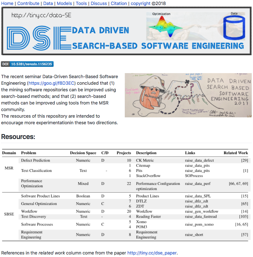
Figure 1. http://tiny.cc/data-se

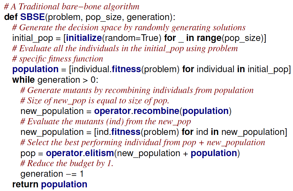
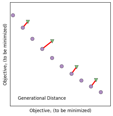
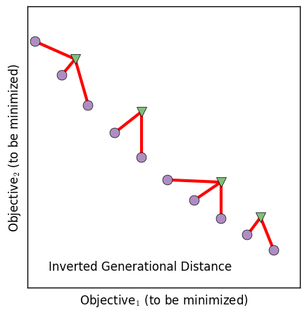
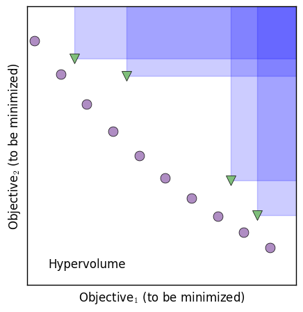
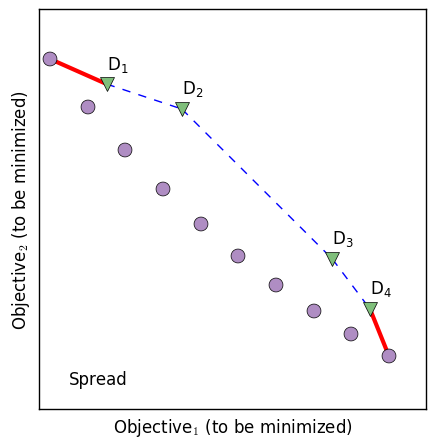
Problems in Search-based Software Engineering   Problem: SBSE converts a SE problem into an optimization problem, where the goal is to find the maxima or minima of objective functions $y_{i}=f_{i}(x)$, $1\leq i\leq m$, where $f_{i}$ are the objective / evaluation functions, $m$ is the number of objectives, x is called the independent variable, and $y_{i}$ are the dependent variables. Global Maximum/Minimum: For single objective ($m=1$) problems, algorithms aim at finding a single solution able to optimize the objective function, i.e., a global maximum/minimum. Pareto Front: For multi-objective ($m>1$) problems, there is no single ‘best’ solution, but a number of ‘best’ solutions. The best solutions are non-dominated solutions found using a dominance relation. Dominance: The domination criterion can be defined as: “A solution $x_{1}$ is said to dominate another solution $x_{2}$, if $x_{1}$ is no worse than $x_{2}$ in all objectives and $x_{1}$ is strictly better than $x_{2}$ in at least one objective.” A solution is called non-dominated if no other solution dominates it. Actual Pareto Front (PF): A list of best solutions of a space is called Actual PF ($a\in A$). As this can be unknowable in practice or prohibitively expensive to generate, it is common to take from the union of all optimization outcomes all non-dominated solutions and use it as the (approximated) PF. Predicted PF: The solutions found by an optimization algorithm are called the Predicted PF ($p\in P$). Components of Meta-heuristic Algorithms (search-based optimization algorithms such as NSGA-II (Deb et al., 2000), SPEA2 (Zitzler et al., 2001), MOEA/D (Zhang and Li, 2007), AGE (Wagner et al., 2015)) Data Collection or Model building: SBSE process can either rely on a model, which represent a software process (Boehm et al., 1995) or can be directly applied to any software engineering problem including problems which require evaluating a solution by running a specific benchmark (Krall et al., 2015). Representation: This defines how solutions $x$ are represented internally by the algorithm. Examples of representations are Boolean or numerical vectors, but more complicated representations are also possible. The space of all values that can be represented is the Decision Space. Population: A set of solutions maintained by the algorithm using the representation. Initialization: The process of search typically starts by creating random solutions (valid or invalid) (Saber et al., 2017; Chen et al., 2017, 2018; Henard et al., 2015). Fitness Function: A fitness function maps the solution (which is represented using numerics) to a numeric scale (also called as Objective Space) which is used to distinguish between good and not so good solutions. This measure is a domain-specific measure (single objective) or measures (multi-objective) which is useful for the practitioners. Simply put fitness function is a transformation function which converts a point in the decision space to the objective space. Operators: These are operators that (1) generate new solutions based on one (e.g., mutation operator) or more (e.g., crossover or recombination operators) existing solutions, and (2) operators that select solutions to pass to the aforementioned operators or to survive for the next iteration of the algorithm. The operators (2) typically apply some pressure towards selecting better solutions either deterministically (e.g., elitism operator) or stochastically. Elitism operator simulates the ‘survival of the fittest’ strategy, i.e., eliminates not so good solutions thereby preserving the good solutions in the population. Generations: A meta-heuristic algorithm iteratively improves the population (set of solutions) iteratively. Each step of this process, which includes generation of new solutions using recombination of the existing population and selecting solutions using the elitism operator, is called a generation. Over successive generations, the population ‘evolves’ toward an optimal solution. Performance Measures (Refer to (Wang et al., 2016a; Chand and Wagner, 2015) for more detail) For single objective problems, measures such as absolute residual or rank-difference can be very useful and cannot be used for multi-objective problems. The following are the measures used for such problems. Generational Distance: Generational distance is the measure of convergence—how close is the predicted Pareto front is to the actual Pareto front. It is defined to measure (using Euclidean distance) how far are the solutions that exist in $P$ from the nearest solutions in $A$. In an ideal case, the GD is 0, which means the predicted PF is a subset of the actual PF. Note that it ignores how well the solutions are spread out. Spread: Spread is a measure of diversity—how well the solutions in P are spread. An ideal case is when the solutions in P is spread evenly across the Predicted Pareto Front. Inverted Generational Distance: Inverted Generational distance measures both convergence as well as the diversity of the solutions—measures the shortest distance from each solution in the Actual PF to the closest solution in Predicted PF. Like Generational distance, the distance is measured in Euclidean space. In an ideal case, IGD is 0, which means the predicted PF is same as the actual PF. Hypervolume: Hypervolume measures both convergence as well as the diversity of the solutions—hypervolume is the union of the cuboids w.r.t. to a reference point. Note that the hypervolume implicitly defines an arbitrary aim of optimization. Also, it is not efficiently computable when the number of dimensions is large, however, approximations exist. Approximation: Additive/multiplicative Approximation is an alternative measure which can be computed in linear time (w.r.t. to the number of objectives). It is the multi-objective extension of the concept of approximation encountered in theoretical computer science.

Figure 2. A brief tutorial on Search-based Software Engineering.

Features	MSR	SBSE
Primary inference	Induction, summarization, visualization	Optimization
Inference speed	Very fast, scalable	Becoming faster, more scalable
Data often collected	Once, then processed.	On-demand from some model—which means an SBSE analysis can generate new samples of the data in very specific regions.
Conclusions often generated via	A single execution of a data miner or an ensemble, perhaps after some data pre-processing.	An evolutionary process where, many times, execution $i+1$ is guided by the results of execution $i$.
Canonical tools are usually	Data mining algorithms like the decision tree learners of WEKA (Hall et al., 2009) or the mathematical modeling tools of R (R Core Team, 2018) or Scikit-learn (Pedregosa et al., 2011).	Search-based optimization algorithms which may be either home-grown scripts or parts of large toolkits such as jMETAL(Durillo and Nebro, 2011), Opt4j (Lukasiewycz et al., 2011), DEAP (Fortin et al., 2012).
Canonical problems	Defect prediction (Lessmann et al., 2008) or Stackoverflow text mining (Fu and Menzies, 2017a).	Minimizing a test suite (Fraser and Wotawa, 2007), configuring a software system (Nair et al., 2017a) or extracting a valid products from a product line description (Sayyad et al., 2013a).
Results assessed by	A small number of standard measures including recall, precision, or false alarm rates (for discrete classes) or magnitude of relative error (for continuous classes) (Shepperd and MacDonell, 2012).	A wide-variety of domain-specific objectives. Whatever the specific objectives, a small number meta-measures are used in many research papers such as the Hypervolume or Spread.

Figure 3. Differences between MSR and Search-based Software Engineering.

Some goals relate to aspects of defect prediction: (1) Mission-critical systems are risk-averse and may accept very high false alarm rates, just as long as they catch any life-threatening possibility. That is, such projects do not care about effort- they want to maximize recall regardless of any impact that might have on the false alarm rate. (2) Suppose a new hire wants to impress their manager. That the new hire might want to ensure that no result presented to management contains true negative; i.e., they wish to maximize precision. (3) Some communities do not care about low precision, just as long as a small fraction the data is returned. Hayes, Dekhytar, & Sundaram call this fraction selectivity and offer an extensive discussion of the merits of this measure (Hayes et al., 2006).

Beyond defect prediction are other goals that combine defect prediction with other economic factors: (4) Arisholm & Briand (Arisholm and Briand, 2006), Ostrand & Weyeuker (Ostrand et al., 2004) and Rahman et al. (Rahman et al., 2012) say that a defect predictor should maximize reward; i.e., find the fewest lines of code that contain the most bugs. (5) In other work, Lumpe et al. are concerned about amateur bug fixes (Lumpe et al., 2011). Such amateur fixes are highly correlated to errors and, hence, to avoid such incorrect bug fixes; we have to optimize for finding the most number of bugs in regions that the most programmers have worked with before. (6) In better-faster-cheaper setting, one seeks project changes that lead to fewer defects and faster development times using fewer resources (El-Rawas and Menzies, 2010; Menzies et al., 2007, 2009; Menzies et al., 2009). (7) Sayyad (Sayyad et al., 2013b, a) explored models of software product lines whose value propositions are defined by five objectives.

All the above measures relate to the tendency of a predictor to find something. Another measure could be variability of the predictor. (8) In their study on reproducibility of SE results, Anda, Sjoberg and Mockus advocate using the coefficient of variation ($CV=\frac{stddev}{mean}$). Using this measure, they defined reproducibility as $\frac{1}{CV}$ (Mockus et al., 2009).

Figure 4. Different users value different things.

2. What? (Definitions)

For this paper, we say that MSR covers the technologies explored by many of the authors at the annual Mining Software Repositories conference.

As to search-based software engineering, that term was coined by Jones and Harman (Harman and Jones, 2001) in 2001. Over the years SBSE has been applied to various fields of software engineering for example, requirements (Zhang et al., 2013b; Chen et al., 2017), automatic program repair (Le Goues et al., 2012), Software Product Lines (Chen et al., 2018; Sayyad et al., 2013b; Guo et al., 2017a), Performance configuration optimization (Nair et al., 2017a, b; Guo et al., 2017b; Oh et al., 2017; Nair et al., 2018) to name of few. SBSE has been applied to other fields and has their own surveys such as design (Räihä, 2010), model-driven engineering (Boussaïd et al., 2017), genetic improvement of programs (Petke et al., 2017), refactoring (Mariani and Vergilio, 2017), Testing (Silva et al., 2017; Khari and Kumar, 2017) as well as more general surveys (Clarke et al., 2003; Harman, 2007).

Figure 2 provides a (very) short tutorial on SBSE and Figure 3 characterizes some of the differences between MSR and SBSE.

As to defining DSE, we say it is some system that solves an SE problem as follows:

• It inserts a data miner into an optimizer; or

• It uses an optimizer to improve a data miner.

3. Why? (Synergies of MSR + SBSE)

Consider the following. The MSR community knows how to deal with large datasets. The SBSE community knows how to take clues from different regions of data, then combine them to generate better solutions. If the two ideas were combined, then MSR could be sampling technology to quickly find the regions where SBSE can learn optimizations. If so:

MSR methods can “supercharge” SBSE.

For a concrete example of this “supercharging”, consider active learning with Gaussian Process Models (GPM) used for multi-objective optimization by the machine learning community (Zuluaga et al., 2016). Active learners assume that evaluating one candidate is very expensive. For example, in software engineering, “evaluating” a test suite might mean re-compiling the entire system then re-running all tests. When the evaluation is so slow, an active learner reflects on the examples seen so far to find the next most informative example to evaluate. One way to do this is to use GPMs to find which parts of a model have maximum variance in their predictions (since sampling in such high-variance regions serves to most constrain the model).

The problem with GPMs is that they do not scale beyond a dozen variables (or features) (Wang et al., 2016b). CART, on the other hand, is a data mining algorithm that scales efficiently to hundreds of variables. So Nair et al. recently explored active learning for multi-objective optimization by replacing GPM with one CART tree per objective (Nair et al., 2018). The resulting system was applied to a wide range of software configuration problems found in tiny.cc/data-se. Compared to GPMs, the resulting system ran orders of magnitude faster, found solutions as good or better, and scaled to much larger problems (Nair et al., 2018).

Not only is MSR useful for SBSE, but so too:

SBSE methods can “supercharge” MSR.

The standard example here is parameter tuning. Most data mining algorithms come with tunable parameters that have to be set via expert judgment. Much recent work shows that for MSR problems such as defect prediction and text mining, SBSE can automatically find settings that are far superior to the default settings. For example:

• When performing defect prediction, various groups report that SBSE methods can find new settings that dramatically improve the performance of the learned model (Fu et al., 2016; Tantithamthavorn et al., 2016, 2018).

• When using SMOTE to rebalance data classes, SBSE found that for distance calculations using

  $$d(x,y)=\left(\sum_{i}(x_{i}-y_{i})^{n}\right)^{1/n}$$

  the Euclidean distance of $n=2$ usually works far worse than another distance measure using $n=3$ (Agrawal and Menzies, 2018).

Note that all the above-used case study material is from tiny.cc/data-se.

Another, subtler, benefit of combining MSR+SBSE relates to the exploration of competing objectives. We note that software engineering tasks rarely involve a single goal. For example, when a software engineer is testing a software, he/she may be interested in finding the highest possible number of software defects at the same time as minimizing the time required for testing. Similarly, when a software engineer is planning the development of a software, he/she may be interested in reducing the number of defects, the effort required to develop the software and the cost of the software. The existence of multiple goals necessarily implies that such problems should be solved via a multi-objective optimizer.

There are many such goals. For example, let $\{A,B,C,D\}$ denote the true negatives, false negatives, false positives, and true positives (respectively) found by a software defect detector. Also, let $L_{A}L_{b},L_{c},L_{d}$ be the lines of code seen in the parts of the system that fall into $A,B,C,D$. Given these definitions then

$$\begin{array}[]{r@{~}l}\mathit{pd}=\mathit{recall}=~{}&D/(B+D)\\ \mathit{pf}=~{}&C/(A+C)\\ \mathit{prec}=\mathit{precision}=~{}&D/(D+C)\\ \mathit{acc}=\mathit{accuracy}=~{}&(A+D)/(A+B+C+D)\\ \mathit{support}=~{}&(C+D)/(A+B+C+D)\\ \textit{effort}=~{}&(L_{c}+L_{d})/(L_{a}+L_{b}+L_{c}+L_{d})\\ \mathit{reward}=~{}&\mathit{pd}/\textit{effort}\end{array}$$

.

The critical point here is that, in terms of evaluation criteria, the above are just the tip of the iceberg. Figure 4 lists several other criteria that have appeared recently in the literature. Note that this list is hardly complete– SE has many sub-problems and many of those problems deserve their specialized evaluation criteria.

SBSE is one way to build inference systems that are specialized to specialized evaluation criteria. SBSE systems accept as input some function that assesses examples on multiple criteria (and that function is used to guide the inference of the SBSE tool). Several recent results illustrate the value of using a wider range of evaluation criteria to assess our models:

• Sarro et al. (Sarro et al., 2016) used SBSE tools that assessed software effort estimation tools not only by their predictive accuracy but also by the confidence of those predictions. These multi-objective methods out-performed the prior state-of-the-art in effort estimation. Prior work also used multi-objective methods to boost the predictive performance of ensembles for software effort estimation (Minku and Yao, 2013).

• Agrawal et al. (Agrawal et al., 2018) used SBSE tools to tune text mining tools for StackOverflow. Standard text mining tools can suffer from “order effects” in which changing the order of the training data leads to large-scale changes in the learned clusters. To fix this, Agrawal et al. tuned the background priors of their Latent Dirichlet allocation (LDA) algorithm to maximize the stability of the learned clusters. Classifiers based on these stabilized clusters performed better than those based on the clusters learned by standard LDA.

Table 1. Different problems and associated strategies explored in this paper. The characteristic of the decision space (C/D) represents whether there are continuous or discrete in nature. The column Links represent the URL from where the problems can be download (prefix http://tiny.cc/).

Domain	Problem	Decision Space	C/D	Projects	Description	Links	Related Work
	Defect Prediction	Numeric	D	10	CK Metric	raise_data_defect	(Fu et al., 2016)
				1	Citemap	raise_data_pits
				6	Pits	raise_data_pits
MSR	Text Classification	Text	-	1	StackOverflow	SOProcess	(Agrawal et al., 2018)
	Performance Optimization	Mixed	D	22	Performance Configuration optimization	raise_data_perf	(Nair et al., 2017a, b, 2018)
	Software Product Lines	Boolean	D	5	Product Lines	raise_data_SPL	(Chen et al., 2018)
				7	DTLZ	raise_dtlz_zdt
	General Optimization	Numeric	C	6	ZDT	raise_dtlz_zdt	(Nair et al., 2016)
	Workflow	Numeric	D	20	Workflow	raise_gen_workflow	(Chen and Menzies, 2017)
	Text Discovery	Text	-	4	Reading Faster	raise_data_fastread	(Yu et al., 2016b)
				5	Xomo
	Software Processes	Numeric	C	4	POM3	raise_pom_xomo	(Nair et al., 2016; Chen et al., 2017)
SBSE	Requirement Engineering	Numeric	D	8	Requirement Engineering	raise_short	(Mathew et al., 2017)

4. How? (Resources for Exploring DSE)

In this section, we assume that the reader has been motivated by the above material to start exploring DSE.

Accordingly, in this section, we describe sample tasks that might be used for that exploration. Note that:

• Table 1 summarizes the material presented in this section.

• All these examples were used in recent SE papers; i.e., for all this material, there exists baseline results against which researchers can use to assess their own new ideas comparatively.

• Support material for that exploration (data, models, scripts), is available from tiny.cc/data-se.

Note that we do not assume that the following list of materials covers the spectrum of problems that could be solved by combining MSR with SBSE. In fact, one of the goals of this paper is to encourage researchers to extend this material by posting their materials as pull requests to tiny.cc/data-se.

4.1. Software Product Lines

Problem Domain: SBSE

Problem: With fast-paced development cycle, traditional code-reuse techniques have been infeasible. Now, software companies are moving a software product line model to reduce cost and increase reliability. Companies concentrate on building software out of core components, and quickly use these components with specializations for certain customers. This allows the companies to have a fast turn around time. In a more concrete sense, a software product line (SPL) is a collection of related software products, which share some core functionality (Harman et al., 2014). From a product line, many products can be generated.

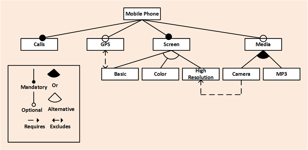
Figure 5. Feature model for mobile phone product line. To form a mobile phone, “Calls” and “Screen” are the mandatory features(shown as solid $\bullet$), while the “GPS” and “Media” features are optimal(shown as hollow $\circ$). The “Screen” feature can be “Basic“, “Color” or “High resolution” (the alternative relationship). The “Media” feature contains “camera”, “MP3”, or both (the Or relationship).

Figure 5 shows a feature model for a mobile phone product line. All features are organized as a tree. The relationship between two features might be “mandatory”, “optional”, “alternative”, or “or”. Also, there exist some cross-tree constraints, which means the preferred features are not in the same sub-tree. These cross-tree constraints complicate the process of exploring feature models. The products are represented as a binary string, where the length of the string is equal to the number of features. A valid product is one which satisfies all the relationship defined in the feature model. Researchers who explore these kinds of models (Sayyad et al., 2013b, a; Harman et al., 2014; Henard et al., 2015) define a “good” product (fitness function) as the one that satisfies five objectives: (1) find the valid products (products not violating any cross-tree constraint or tree structure), (2) with more features, (3) less known defects, (4) less total cost, and (5) most features used in prior applications.

Challenges: Finding a valid product in real-world software product lines can be very difficult due to the sheer scale of these product lines. Some software product line models comprise up to tens of thousands of features, with 100,000s of constraints. These constraints make it difficult to generate valid product through random assignments. In some cases, chances of finding valid solutions through random assignment are $0.04\%$. Most of the meta-heuristic algorithms often fail to find valid solutions or take a long time to find one. Given the large and constrained search space ($2^{N}$, where N is the number of features) using a meta-heuristic algorithm can be infeasible.

Strategy: Since exploring all the possible solutions is expensive and often infeasible, the SWAY, or “Sampling WAY”, clusters the individual products based on their features. Please note, clustering does not require evaluations—to find the fitness of each product. SWAY uses a domain-specific distance function to cluster the points. A domain-specific distance function was required because (1) clusters should have similar products—similar fitness values, and (2) the decision space is a boolean space. This is in line with the observation of Zhang et al. (Zhang et al., 2013a), who reports that MSR practitioners understand the data using domain knowledge. Once the products are clustered, a product is selected (at random) from each cluster. Based on the fitness values of the ‘representative product,’ the not so promising clusters are eliminated. This step is similar to the elitism operator of meta-heuristic algorithms. This process continues recursively till a certain budget is reached. Please refer to (Nair et al., 2016; Chen et al., 2017, 2018) for more details. The reproduction package of SWAY and associated material can be found in http://tiny.cc/raise_spl.

4.2. Performance Configuration Optimization

Problem Domain: MSR

Problem: Modern software systems come with a lot of knobs or configuration options, which can be tweaked to modify the functional or non-functional (e.g., throughput or runtime) requirements. Finding the best or optimal configuration to run a particular workload is essential since there is a significant difference between the best and the worst configurations. Many researchers report that modern software systems come with a daunting number of configuration options (Xu et al., 2015). The size of the configuration space increases exponentially with the number of configuration options. The long runtimes or cost required to run benchmarks make this problem more challenging.

Challenges: Prior work in this area used a machine learning method to accurately model the configuration space. The model is built sequentially, where new configurations are sampled randomly, and the quality or accuracy of the model is measured using a holdout set. The size of the holdout set in some cases could be up to 20% of the configuration space (Nair et al., 2017b) and need to be evaluated (i.e., measured) before even the machine learning model is entirely built. This strategy makes these methods not suitable in a practical setting since the generated holdout set can be (very) expensive. On the other hand, there are software systems for which an accurate model cannot be built.

Strategy: The problem of finding the (near) optimal configuration is expensive and often infeasible using the current techniques. A useful strategy could be to build a machine learning model which can differentiate between the good and not so good solutions. Flash, a Sequential Model-based Optimization (SMBO), is a useful strategy to find extremes of an unknown objective. Flash is efficient because of its ability to incorporate prior belief as already measured solutions (or configurations), to help direct further sampling. Here, the prior represents the already known areas of the search (or performance optimization) problem. The prior can be used to estimate the rest of the points (or unevaluated configurations). Once one (or many) points are evaluated based on the prior, the posterior can be defined. The posterior captures the updated belief in the objective function. This step is performed by using a machine learning model, also called surrogate model. The concept of Flash can be simply stated as:

• Given what one knows about the problem,

• what can be done next?

The “given what one knows about the problem” part is achieved by using a machine learning model whereas “what can be done next” is performed by an acquisition function. Such acquisition function automatically adjusts the exploration (“should we sample in uncertain parts of the search space”) and exploitation (“should we stick to what is already known”) behavior of the method. Please refer to (Nair et al., 2018) and (Nair et al., 2017b, a; Jamshidi and Casale, 2016) to similar strategies. The reproduction package is available in http://tiny.cc/flashrepo/.

4.3. Requirements Models

Problem Domain: SBSE

Problem: The process of building and analyzing complex requirements engineering models can help stakeholders better understand the ramifications of their decisions (van Lamsweerde, 2001; Amyot et al., 2010). But models can sometimes overwhelm stakeholders. For example, consider a committee reviewing a goal model (see fig. 6) that describes the information needs of a computer science department (Horkoff and Yu, 2016). Although the model is entangled, on manual and careful examination, it can be observed that much of the model depends on a few “key” decisions such that once their values are assigned, it becomes very simple to reason over the remaining decisions. It is beneficial to look for these “keys” in requirements models since, if they exist, one can achieve “shorter” reasoning about RE models, where “shorter” is measured as follows:

• Large models can be processed in a short time.

• Runtimes for automatic reasoning about RE models are shorter so stakeholders can get faster feedback on their models.

• The time required for manual reasoning about models is shorter since stakeholders need only debate a small percent of the issues (just the key decisions).

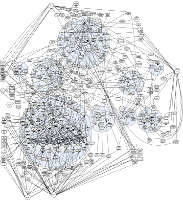
Figure 6. Options for services in a CS department (i* format). It shows how complicated it is to reason about services.

Such models are represented using the i* framework (Yu, 1997) which include the key concepts of NFR (Chung et al., 1992) framework, including soft goals, AND/OR decompositions and contribution links along with goals, resources, and tasks.

Challenges: Committees have trouble with manually reasoning about all the conflicting relationships in models like fig. 6 due to its sheer size and numerous interactions (this model has 351 node, 510 edges and over 500 conflicting relationships). Further, automatic methods for reasoning about these models are hard to scale up: as discussed below, reasoning about inference over these models is an NP-hard task.

Strategy: To overcome this problem, a technique called SHORT was proposed, which runs in four phases:

• SH: ’S’ample ’H’euristically the possible labelings of the model.

• O: ’O’ptimize the label assignments to cover more goals or reduce the sum of the cost of the decisions in the model.

• R: R: ’R’ank all decisions according to how well they performed during the optimization process.

• T: T: ’T’est how much conclusions are determined by the decisions that occur very early in that ranking.

The above technique was used on eight large real-world Requirements Engineering models. It was shown that only under 25% of their decisions are “keys” and 6 of them had less than 12% decisions as keys. The process of identifying keys was also fast as it could run in near linear time with the largest of models running in less than 18 seconds. Please refer to (Mathew et al., 2017) for more details and the reproduction package can be found at http://tiny.cc/raise_short.

4.4. Faster Literature Reviews

Problem Domain: SBSE

Problem: Broad and complete literature reviews.

Data sets and reproduction packages for all the following are available at https://doi.org/10.5281/zenodo.837298 (for Challenge 1) and https://doi.org/10.5281/zenodo.1147678 (for Challenges 2,3,4). Please refer to (Yu et al., 2016a; Yu and Menzies, 2017a) for more details

Challenge 1: Literature reviews can be extremely labor intensive and often require months (if not year) to complete. Due to a large number of papers available, the relevant papers are hard to find. A graduate student needs to review thousands of papers before finding the few dozen relevant ones. Therefore the challenge is: how to maximize relevant information (when there is a lot of noise) while minimizing the search cost to find relevant information?

Strategy: Reading all literature is unfeasible. To selectively read the most informative literature, active learners are applied—which incrementally learns from the human feedback and suggests on which paper to review next (Yu and Menzies, 2018).

Challenge 2: A wrong choice of initial papers can increase the review effort by up to 300% than the median effort (repeat for 30 runs)—requires three times more effort to find relevant papers (Yu and Menzies, 2017b).

Strategy: Reduce variances by selecting a good initial set of papers with domain knowledge from the researcher. It is found that by ranking the papers with some keywords (provided as domain knowledge) and reviewing in such order, the effort can be reduced with negligible variances (Yu and Menzies, 2017a).

Challenge 3: When to stop?. If too early then many relevant papers will be missed else much time will be wasted on irrelevant papers.

Strategy: Use a semi-supervised machine learning algorithm (Logistic Regression) to learn from the search process (till now) to predict how much more relevant paper will be found (Yu and Menzies, 2017a).

Challenge 4: Research shows that it is reasonable to assume the precision and recall of a human reviewer are around 70%. When such human errors occur, how to correct the errors so that the active learner is not misled?

Strategy: Concentrate the effort on correctly classifying the paper which creates the most controversy. Using this intuition, periodically few of the already evaluated papers, whose labels the active learner disagree most on, are re-evaluated (Yu and Menzies, 2017a).

4.5. Text classification

Problem Domain: MSR

Problem: Stack Overflow is a popular Q&A website, where users posts the questions and the community collectively answers these questions. However, as the community evolves, there is a chance that duplicate questions can appear—which results in a wasted effort of the community. There is a need to remove the duplicate question or consolidate related questions. The problem focuses on discovering the relationship between any two questions posted on Stack Overflow and classifies them into duplicates, direct link, indirect link, and isolated (Fu and Menzies, 2017a; Xu et al., 2016). One way to solve this problem is to build a predictive model to predict the similarity between two questions.

Challenge: The state-of-the-art method for this problem used Deep Learning, which was expensive to train (Xu et al., 2016). For example, Xu et al. spent 14 hours on training a deep learning model. Such long training time is not appropriate for the field of software analytics since software analytics requires the methods to have a fast turnaround time (Zhang et al., 2013a).

Strategy: To reduce the training time as well as promote simplicity, hyper-parameter optimization of simple learners, like SVM (Support Vector Machines), is a way to go. Specifically, a meta-heuristic algorithm called Differential Evolution, which has been an effective tuning algorithm (used in SBSE) (Fu et al., 2016), was used to explore the parameter space of SVM. After the search process, SVM with best-found parameters is used to predict classes of Stack Overflow questions. This method can get similar or better results than the deep learning method while reducing the training time by up to 80 times. Please refer to (Fu and Menzies, 2017a) for more details and the reproduction package can be found in http://tiny.cc/raise_data_easy.

Figure 7. Some of cloud computing workflows. Clockwise from top left: Montage, Epigenomics, Inspiral, CyberShake, Sipht. Each node is one “task” and each edge is a data flow from one task to another. Number of tasks can vary from dozens to thousands).

4.6. Workflows in Cloud Environment

Problem Domain: SBSE

Problem: Many complex computational tasks, especially in a scientific area, can be divided into several sub-tasks where outputs of some tasks serves as the input to another. A workflow is a tool to model such kind of computational tasks.

Figure 7 shows five types of widely studied workflows. Workflows are represented as a directed acyclic graph (DAG). Each vertex of the DAGs represents one sub-task. Connections between vertices represent the result communications between different vertices. One computational task is called “finished” only when all sub-tasks are finished. Also, sub-tasks should follow the constraints per edges.

Grid computing techniques, invented in the mid-1990s, as well as recently lots of pay-as-you-go cloud computing services, e.g., Amazon EC2, provide researchers a feasible way to finish such kind of complicated workflow in a reasonable time. The workflow configuring problem is to figure out the best deployment configurations onto a cloud environment. The deployment configuration contains (1) determine which sub-tasks can be deployed into one computation node, i.e., the virtual machine in cloud environment; (2) which sub-task should be executed first if two of them are to be executed in the same node; (3) what hardware configuration (CPU, memory, bandwidth, etc.) should be applied in each computation node. Commercial cloud service provider charges users for computing resource. The objective of cloud configuration is to minimize the monetary cost as well as minimize the runtime of computing tasks.

Challenges: The two reasons that make workflow configuration on cloud environment challenging are: (1) some sub-tasks of workflows can be as large as hundreds, or thousands; also, sub-tasks are under constraints– file flow between them. (2) available types of computing nodes from cloud service providers are large. For example, Amazon AWS provides more than 50 types of virtual machines; these virtual machines have different computing ability, as well as unit price (from $0.02/hr to $5/hr). Given these two reasons, the configuration space, or some possible deployment ways, is large. Even though modern cloud environment simulator, such as CloudSim, can quickly access performance of one deployment, evaluate every possible deployment configuration is impossible.

Strategy: Since it is impossible to enumerate all possible configurations, most existed algorithm use either (1) greedy algorithm (2) evolutionary algorithm to figure out best configurations. Similar to other search-based software engineering problems, these methods require a large number of model evaluations (simulations in workflow configuration problem). The RIOT, or randomized instance-order-type, is an algorithm to balance execution time as well as cost in a short time. The RIOT first groups sub-tasks, making the DAG simpler, and then assign each group into one computation node. Within one node, priorities of sub-tasks are determined by B-rank (Topcuoglu et al., 2002), a greedy algorithm. The most tricky part is to determine types of computation nodes so that they can coordinate with each other and reduce the total ideal time (due to file transfer constraints). RIOT makes full use of two hypothesis: (1) similar configurations should have similar performance and (2) (monotonicity) k times computing resource should lead to (1/k)*c less computation time (where c is constant for one workflow). With these two hypotheses, RIOT first randomly creates some deployment configurations and evaluates them, then guess more configurations based on current evaluated configuration. Such kind of guess can avoid a large number of configuration evaluations. Please refer to (Chen and Menzies, 2017) for more details and the reproduction package is available in http://tiny.cc/raise_gen_workflow.

5. Practical Guidelines

Based on our experiences this section lists practical guidelines for those who are familiar with MSR (but not with SBSE) to be able to work on DSE. Though one would expect exceptions or probably simpler techniques, given the current techniques listed in this paper (Section 4), we believe that it is essential to provide practical guidance that will be valid in most cases and enable practitioners to use these techniques to solve their problems. We recommend that practitioners follow these guidelines and possibly use them as a teaching resource.

Learning: To learn SBSE, coding up a Simulated Annealer (Van Laarhoven and Aarts, 1987) and Differential Evolution (DE) (Storn and Price, 1997) is a good starting point. These algorithms work well for single-objective problems. For multi-objective problems, one should code up binary domination and indicator domination (Zitzler et al., 2001). Note that the indicator domination is recommended for N¿2 objectives and that indicator domination along with DE can find a wide spread of solutions on the PF.

As to learning more about area, the popular venues are:

• GECCO: The Genetic and Evolutionary Computation Conference (which has a special SBSE track);

• TSE: IEEE Transactions on Evolutionary Computation;

• SSBSE: the annual symposium on search-based SE;

• Recent papers at FSE, ICSE, ASE, etc: goo.gl/Lvb42Z;

• Google Scholar: see goo.gl/x44u77.

Debugging: It is always recommended to use small and simple optimization problems for the purposes of debugging. For example, small synthetic problems like ZDT, DTLZ (Deb et al., 2005), and WFG (Huband et al., 2006) are very useful to evaluate a meta-heuristic algorithm. For further details about other test problems, please refer to (Huband et al., 2006).

That said, it is not recommended that you try publishing results based on these small problems. In our experience, SE reviewers are more interested in results from the resources listed in Table 1, rather than results from synthetic problems like ZDT, DTLZ, and WFG. Instead, it is better to publish results on interesting problems taken from the SE literature, such as those shown in Section 4.

Another aspect of debugging is to notice the gradual improvement of results in terms of the performance metrics. In most cases, the performance metric for generation $n$ would be worse than generation $n+\delta$, where $\delta$ is a positive integer. In an unstable meta-heuristic algorithm, the performance metrics fluctuate a lot between generations. It is also common to observe a fitness curve over generations where the fitness initially improves more quickly and then starts to converge. However, a typical undesired result is premature convergence, which occurs when the algorithm converges rapidly too to poor local optimal solutions.

Normalization: When working with multi-objective problems, it is important to normalize the objective space to eliminate scaling issues. For example, Ishibuchi et al. (Ishibuchi et al., 2017) showed that WFG4-9 test problems (Huband et al., 2006), the range of the Pareto front on the $i^{th}$ objective is $[0,2i]$. This means that the tenth objective has a ten times wider range than the first objective. It is difficult for meta-heuristic algorithm without normalization to find a set of uniformly distributed solutions over the entire Pareto front for such a many-objective test problem.

Choosing Algorithm and its parameters: Choosing the meta-heuristic algorithm to solve a particular problem can often be challenging. Although the chosen algorithm is a preference of the researcher, it is commonly agreed to use NSGA-II or SPEA2 for problems with less than 3 objectives whereas NSGA-III and MOEA/D is preferred for problems with more than 3 objectives.

Choosing the correct parameters of a meta-heuristic algorithm are essential for its performance. There are various rules of thumb, which are proposed by various researchers such as population size is the most significant parameter and that the crossover probability and mutation rate have insignificant effects on the GA performance (Alajmi and Wright, 2014). However, we recommend using a simple tuner to find the best parameter for the meta-heuristic algorithms. Tuners could be something as simple as Differential Evolution or Grid Search.

Experimentation: We recommend an experimentation technique called (you+two+next+dumb), defined as

• “you” is your new method;

• “two” well-established methods (often NSGA-II and SPEA2),

• a “next” generation method e.g. MOEA/D (Zhang and Li, 2007), NSGA-III (Deb and Jain, 2014),

• one “dumb” baseline method (random search or SWAY).

While comparing a new meta-heuristic algorithm or a DSE technique, it is essential to baseline it with the simplest baseline such as a random search. Bergestra et al. (Bergstra and Bengio, 2012) demonstrated that random search which uses same computational budget finds better solutions by effectively searching a larger, less promising configuration space. Another alternative could be to generate numerous random solutions and reject less promising solutions using domain-specific heuristics. Chen et al. (Chen et al., 2018), showed that SWAY—oversampling and subsequent pruning less promising solutions, is competitive with state-of-the-art solutions. Baselines like random search or SWAY can help researchers and industrial practitioners by achieving fast early results while providing ‘hints’ for subsequent experimentation. Another important aspect is to compare the performance of the new technique with the current state-of-the-art techniques. Well established techniques in the SBSE literature are NSGA-II and SPEA2 (Chen et al., 2017). Please note that the state-of-the-art techniques differs among the various sub-domains.

Reporting results: Meta-heuristic algorithms in SBSE are an intelligent modification of a randomized algorithm. Like randomized algorithms, the meta-heuristic algorithms may be strongly affected by chance. Running a randomized algorithm twice on the same problem usually produces different results. Hence, it is imperative to run the meta-heuristic algorithm multiple times to capture the behavior of an algorithm. Arcuri et al. (Arcuri and Briand, 2011) reports that meta-heuristic algorithms should be run at least 30 times. Take special care to use different random seeds for running each iteration of the algorithms. This makes sure that the randomness is accounted for while reporting the results. To analyze the effectiveness of a meta-heuristic algorithm, it is important to study the distribution of its performance metrics. A practitioner might be tempted to use the average (mean) of the performance metrics to compare the effectiveness of different algorithms. However, given the variance of the performance metrics between different runs just looking only at average values can be misleading. For detecting statistical differences and compare central tendencies and overall distributions, use of non-parametric statistical methods such as Scott-Knott using bootstrap and cliffs delta for the significance and effect size test (Mittas and Angelis, 2013; Ghotra et al., 2015), Friedman (Lessmann et al., 2008) or Mann-Whitney U-test (Arcuri and Briand, 2011)– please refer to (Arcuri and Briand, 2011, 2014).

Replication Packages: As a community, we advance by accumulating knowledge built upon observations of various researchers. We believe that replicating an experiment (thereby observations) many times transforms evidence into a trusted result. The goal of any research should be not the running of individual studies but developing a better understanding of process and debate about various strength and weakness of the approach. In the experiments with DSE, there are many uncontrollable sources of variation exist from one research group to another for the results of any study, no matter how well run, to be extrapolated to other domains.

Along with increasing the confidence of a certain observation, it also increases the speed of research. For example, recently in FSE’17, Fu et al. (Fu and Menzies, 2017b) described the effects of arxiv.org or the open science effect. Fu et al. described how making the paper, and the replication packages publicly available, results in 5 different techniques (each superior to its predecessor). Please see http://tiny.cc/unsup for more details on arxiv.org effect.

Hence, it is essential to make replication packages available. In our experience, we have found that replication packages hosted on personal web pages tend to disappear or end up with dead links after a few years. We have found that storing replication packages and artifacts on Github and registering it with Zenodo (https://zenodo.org) is an effective strategy. Note that once registered, then every new release (on Github) will be backed up on Zenodo and made available. Also considering posting a link to your package on tiny.cc/data-se, which is a more curated list.

6. Open Research Issues

We hope this article inspires a larger group of researchers to work on open, and compelling problems in DSE. There are many such problems, including the few listed below.

Explanation: SBSE is often instance-based and provide optimal or (near) optimal solutions. This is not ideal since it provides no insight into the problem. However, using MSR techniques finding building blocks of good solutions may shed light on the relationship different parameters that affect the quality of a solution. This is an important shortcoming of SBSE which have not been addressed by this community. Valerdi notes that, without automated tools, it can take days for human experts to review just a few dozen examples. In that same time, an automatic tool can explore thousands to billions of more solutions. Humans can find it an overwhelming task just to certify the correctness of conclusions generated from so many results. Verrappa and Leiter warn that: “… for industrial problems, these algorithms generate (many) solutions which make the task of understanding them and selecting one amongst them difficult and time-consuming.” (Veerappa and Letier, 2011). Currently, there has been only a few efforts to comprehend the results of an SBSE technique. Nair et al. (Nair et al., 2017c) uses a domination tree along with a Bayesian-based method to better, and more succinctly, explain the search space.

Human in the loop: Once we have explanation running, then the next step would be to explore combinations of human and artificial intelligence for enhanced DSE. Standard genetic algorithms must evaluate 1000s to 1,000,000s of examples– which makes it hard for engineers or business users to debug or audit the results of that analysis. On the other hand, tools like FLASH (described in the last bullet) and SWAY (see Section 4.1) only evaluated $O(log(N))$ of the candidates– which in practice can be just a few dozen examples. This number is small enough to ask humans to watch the reasoning and, sometimes, catch the SBSE tool making mistakes as it compares alternatives. This style of human in the loop reasoning could be used for many tasks such as:

• Debugging or auditing the reasoning.

• Enhancing the reasoning; i.e., can human intelligence, applied judiciously, boost artificial intelligence?

• Checking for missing attributes: when human experts say two identical examples are different, we can infer that there are extra attributes, not currently being modeled, that are important.

• Increasing human confidence in the reasoning by tuning, a complex process, into something humans can monitor and understand.

Transfer Learning: The premise of software analytics is that there exists data from the predictive model can be learned. However in the cases where data is scarce, sometimes it is possible to use data collected from same or other domains which can be used for building predictive models. There is some recent work exploring the problem of transferring data from one domain to another for data analytics. These research have focused on two methodological variants of transfer learning: (a) dimensionality transform based techniques (Nam et al., 2013; Krishna et al., 2016; Nam et al., 2017; Minku and Yao, 2014) and (b) the similarity based approaches (Kocaguneli and Menzies, 2011; Kocaguneli et al., 2015; Peters et al., 2015). These techniques can be readily applied to SBSE to reduce further the cost of finding the optimal solutions. For example, while searching for the right configuration for a specific workload ($w_{a}$), we could reuse measurement from a prior optimization exercise, which uses a different workload ($w_{b}$), to further prune the search space (Jamshidi et al., 2017, 2017; Valov et al., 2017).

Optimizing Optimizers: Many of the methods above can be used to tune approaches. However, many of them experience difficulties once the underlying function is noisy or the algorithm stochastic (and thus the optimizer gets somewhat misleading feedback), once many parameters are to be tuned, or once the approach is to be tuned for large corpora of instances where the objectives vary significantly. Luckily, in recent years, many automated parameter optimization methods have been developed and published as software packages. General purpose approaches include ParamILS (Hutter et al., 2007), SMAC (Hutter et al., 2011), GGA (Ansótegui et al., 2009)), and the iterated f-race procedure called irace (Birattari et al., 2002). Of course, even such algorithm optimizers can be optimized further. One word of warning: as algorithm tuning is already computationally expensive, the tuning of algorithm tuners is even more so. While Dang et al. (Dang et al., 2017) recently used surrogate functions to speed up the optimizer tuning, more research is needed for the optimization of optimizers more widely applicable. Lastly, an alternative to the tuning of algorithms is that of selecting an algorithm from a portfolio or determining an algorithm configuration, when an instance is given. This typically involves the training of machine learning models on performance data of algorithms in combination with instances given as feature data. In software engineering, this has been recently used as a DSE approach for the Software Project Scheduling Problem (Shen et al., 2018; Wu et al., 2016). The field of per-instance configuration has received much attention recently, and we refer the interested reader to a recent updated survey article (Kotthoff, 2016).

7. Conclusions

SE problems can be solved both by MSR and SBSE techniques, but both these methods have their shortcomings. This paper has argued these shortcomings can be overcome by merging ideas from both these domains, to give rise to a new field of software engineering called DSE. This sub-area of SE boosts the techniques used in MSR and SBSE by drawing inspiration from the other field.

This paper proposes concrete strategies which can be used to combine the techniques from MSR and SBSE to solve an SE problem. It also list resources which researchers can use to jump-start their research. One of the aims of the paper is to provide resources and material which can be used as teaching or training resources for a new generation of researchers.

References

- [1]
- Agrawal et al. [2018] Amritanshu Agrawal, Wei Fu, and Tim Menzies. 2018. What is Wrong with Topic Modeling?(and How to Fix it Using Search-based Software Engineering). Information and Software Technology (2018).
- Agrawal and Menzies [2018] Amritanshu Agrawal and Tim Menzies. 2018. ” Better Data” is Better than” Better Data Miners”(Benefits of Tuning SMOTE for Defect Prediction). International Conference on Software Engineering (2018).
- Alajmi and Wright [2014] Ali Alajmi and Jonathan Wright. 2014. Selecting the most efficient genetic algorithm sets in solving unconstrained building optimization problem. International Journal of Sustainable Built Environment (2014).
- Amyot et al. [2010] Daniel Amyot, S Ghanavati, Jennifer Horkoff, G Mussbacher, L Peyton, and Eric S K Yu. 2010. Evaluating Goal Models within the Goal-oriented Requirement Language. International Journal of Intelligent Systems (2010).
- Ansótegui et al. [2009] Carlos Ansótegui, Meinolf Sellmann, and Kevin Tierney. 2009. A Gender-Based Genetic Algorithm for the Automatic Configuration of Algorithms.
- Arcuri and Briand [2011] Andrea Arcuri and Lionel Briand. 2011. A practical guide for using statistical tests to assess randomized algorithms in software engineering. In International Conference on Software Engineering.
- Arcuri and Briand [2014] Andrea Arcuri and Lionel Briand. 2014. A hitchhiker’s guide to statistical tests for assessing randomized algorithms in software engineering. Software Testing, Verification and Reliability (2014).
- Arisholm and Briand [2006] E. Arisholm and L. Briand. 2006. Predicting Fault-prone Components in a Java Legacy System. In 5th ACM-IEEE International Symposium on Empirical Software Engineering.
- Bergstra and Bengio [2012] James Bergstra and Yoshua Bengio. 2012. Random search for hyper-parameter optimization. Journal of Machine Learning Research (2012).
- Birattari et al. [2002] Mauro Birattari, Thomas Stützle, Luis Paquete, and Klaus Varrentrapp. 2002. A Racing Algorithm for Configuring Metaheuristics. In Genetic and Evolutionary Computation Conference.
- Boehm et al. [1995] Barry Boehm, Bradford Clark, Ellis Horowitz, Chris Westland, Ray Madachy, and Richard Selby. 1995. Cost models for future software life cycle processes: COCOMO 2.0. Annals of software engineering (1995).
- Boussaïd et al. [2017] Ilhem Boussaïd, Patrick Siarry, and Mohamed Ahmed-Nacer. 2017. A survey on search-based model-driven engineering. Automated Software Engineering (2017).
- Chand and Wagner [2015] Shelvin Chand and Markus Wagner. 2015. Evolutionary many-objective optimization: A quick-start guide. Surveys in Operations Research and Management Science (2015).
- Chen and Menzies [2017] Jianfeng Chen and Tim Menzies. 2017. RIOT: a Novel Stochastic Method for Rapidly Configuring Cloud-Based Workflows. arXiv preprint arXiv:1708.08127 (2017).
- Chen et al. [2018] J. Chen, V. Nair, R. Krishna, and T. Menzies. 2018. ”Sampling” as a Baseline Optimizer for Search-based Software Engineering. IEEE Transactions on Software Engineering (2018).
- Chen et al. [2017] Jianfeng Chen, Vivek Nair, and Tim Menzies. 2017. Beyond evolutionary algorithms for search-based software engineering. Information and Software Technology (2017).
- Chung et al. [1992] Lawrence Chung, John Mylopoulos, and Brian A Nixon. 1992. Representing and Using Nonfunctional Requirements: A Process-Oriented Approach. IEEE Transactions on Software Engineering (1992).
- Clarke et al. [2003] John Clarke, Jose Javier Dolado, Mark Harman, Rob Hierons, Bryan Jones, Mary Lumkin, Brian Mitchell, Spiros Mancoridis, Kearton Rees, Marc Roper, and others. 2003. Reformulating software engineering as a search problem. IEE Proceedings-software (2003).
- Dang et al. [2017] Nguyen Dang, Leslie Pérez Cáceres, Patrick De Causmaecker, and Thomas Stützle. 2017. Configuring Irace Using Surrogate Configuration Benchmarks. In Genetic and Evolutionary Computation Conference.
- Deb et al. [2000] Kalyanmoy Deb, Samir Agrawal, Amrit Pratap, and Tanaka Meyarivan. 2000. A fast elitist non-dominated sorting genetic algorithm for multi-objective optimization: NSGA-II. In International Conference on Parallel Problem Solving From Nature.
- Deb and Jain [2014] Kalyanmoy Deb and Himanshu Jain. 2014. An evolutionary many-objective optimization algorithm using reference-point-based nondominated sorting approach, part I: Solving problems with box constraints. IEEE Transaction on Evolutionary Computation (2014).
- Deb et al. [2005] Kalyanmoy Deb, Lothar Thiele, Marco Laumanns, and Eckart Zitzler. 2005. Scalable test problems for evolutionary multiobjective optimization. Evolutionary Multiobjective Optimization. Theoretical Advances and Applications (2005).
- Durillo and Nebro [2011] Juan J. Durillo and Antonio J. Nebro. 2011. jMetal: A Java Framework for Multi-objective Optimization. Journal of Advances in Engineering Software (2011).
- El-Rawas and Menzies [2010] Oussama El-Rawas and Tim Menzies. 2010. A Second Look at Faster, Better, Cheaper. Innovations Systems and Software Engineering (2010).
- Fortin et al. [2012] Félix-Antoine Fortin, François-Michel De Rainville, Marc-André Gardner, Marc Parizeau, and Christian Gagné. 2012. DEAP: Evolutionary Algorithms Made Easy. Journal of Machine Learning Research 13 (jul 2012), 2171–2175.
- Fraser and Wotawa [2007] Gordon Fraser and Franz Wotawa. 2007. Redundancy based test-suite reduction. Fundamental Approaches to Software Engineering (2007).
- Fu and Menzies [2017a] Wei Fu and Tim Menzies. 2017a. Easy over Hard: A Case Study on Deep Learning. arXiv preprint arXiv:1703.00133 (2017).
- Fu and Menzies [2017b] Wei Fu and Tim Menzies. 2017b. Revisiting Unsupervised Learning for Defect Prediction. arXiv preprint arXiv:1703.00132 (2017).
- Fu et al. [2016] Wei Fu, Tim Menzies, and Xipeng Shen. 2016. Tuning for software analytics: Is it really necessary? Information and Software Technology (2016).
- Ghotra et al. [2015] Baljinder Ghotra, Shane McIntosh, and Ahmed E Hassan. 2015. Revisiting the impact of classification techniques on the performance of defect prediction models. In Proceedings of the 37th International Conference on Software Engineering-Volume 1. IEEE Press, 789–800.
- Guo et al. [2017a] Jianmei Guo, Jia Hui Liang, Kai Shi, Dingyu Yang, Jingsong Zhang, Krzysztof Czarnecki, Vijay Ganesh, and Huiqun Yu. 2017a. SMTIBEA: a hybrid multi-objective optimization algorithm for configuring large constrained software product lines. Software & Systems Modeling (2017).
- Guo et al. [2017b] Jianmei Guo, Dingyu Yang, Norbert Siegmund, Sven Apel, Atrisha Sarkar, Pavel Valov, Krzysztof Czarnecki, Andrzej Wasowski, and Huiqun Yu. 2017b. Data-efficient performance learning for configurable systems. Empirical Software Engineering (2017).
- Hall et al. [2009] Mark Hall, Eibe Frank, Geoffrey Holmes, Bernhard Pfahringer, Peter Reutemann, and Ian H Witten. 2009. The WEKA data mining software: an update. ACM SIGKDD explorations newsletter (2009).
- Harman [2007] Mark Harman. 2007. The current state and future of search based software engineering. In 2007 Future of Software Engineering.
- Harman et al. [2014] Mark Harman, Yue Jia, Jens Krinke, William B Langdon, Justyna Petke, and Yuanyuan Zhang. 2014. Search based software engineering for software product line engineering: a survey and directions for future work. In International Software Product Line Conference.
- Harman and Jones [2001] Mark Harman and Bryan F Jones. 2001. Search-based software engineering. Information and software Technology (2001).
- Hayes et al. [2006] Jane Huffman Hayes, Alex Dekhtyar, and Senthil Karthikeyan Sundaram. 2006. Advancing Candidate Link Generation for Requirements Tracing: The Study of Methods. IEEE Trans. Software Eng (2006).
- Henard et al. [2015] Christopher Henard, Mike Papadakis, Mark Harman, and Yves Le Traon. 2015. Combining multi-objective search and constraint solving for configuring large software product lines. In International Conference on Software Engineering.
- Horkoff and Yu [2016] Jennifer Horkoff and Eric Yu. 2016. Interactive goal model analysis for early requirements engineering. Requirements Engineering (2016).
- Huband et al. [2006] Simon Huband, Philip Hingston, Luigi Barone, and Lyndon While. 2006. A review of multiobjective test problems and a scalable test problem toolkit. IEEE Transactions on Evolutionary Computation (2006).
- Hutter et al. [2011] Frank Hutter, Holger H. Hoos, and Kevin Leyton-Brown. 2011. Sequential Model-Based Optimization for General Algorithm Configuration.
- Hutter et al. [2007] Frank Hutter, Holger H. Hoos, and Thomas Stützle. 2007. Automatic Algorithm Configuration Based on Local Search. In National Conference on Artificial Intelligence.
- Ishibuchi et al. [2017] Hisao Ishibuchi, Ken Doi, and Yusuke Nojima. 2017. On the effect of normalization in MOEA/D for multi-objective and many-objective optimization. Complex & Intelligent Systems (2017).
- Jamshidi and Casale [2016] Pooyan Jamshidi and Giuliano Casale. 2016. An uncertainty-aware approach to optimal configuration of stream processing systems. In International Symposium on Modeling, Analysis and Simulation of Computer and Telecommunication Systems.
- Jamshidi et al. [2017] Pooyan Jamshidi, Miguel Velez, Christian Kästner, Norbert Siegmund, and Prasad Kawthekar. 2017. Transfer learning for improving model predictions in highly configurable software. In Symposium on Software Engineering for Adaptive and Self-Managing Systems.
- Khari and Kumar [2017] Manju Khari and Prabhat Kumar. 2017. An extensive evaluation of search-based software testing: a review. Soft Computing (2017).
- Kocaguneli and Menzies [2011] Ekrem Kocaguneli and Tim Menzies. 2011. How to find relevant data for effort estimation?. In Symposium on Empirical Software Engineering and Measurement.
- Kocaguneli et al. [2015] Ekrem Kocaguneli, Tim Menzies, and Emilia Mendes. 2015. Transfer learning in effort estimation. Empirical Software Engineering (2015).
- Kotthoff [2016] Lars Kotthoff. 2016. Algorithm Selection for Combinatorial Search Problems: A Survey.
- Krall et al. [2015] Joseph Krall, Tim Menzies, and Misty Davies. 2015. Gale: Geometric active learning for search-based software engineering. IEEE Transactions on Software Engineering (2015).
- Krishna et al. [2016] Rahul Krishna, Tim Menzies, and Wei Fu. 2016. Too much automation? The bellwether effect and its implications for transfer learning. In Automated Software Engineering.
- Le Goues et al. [2012] Claire Le Goues, ThanhVu Nguyen, Stephanie Forrest, and Westley Weimer. 2012. Genprog: A generic method for automatic software repair. IEEE Transactions on Software Engineering (2012).
- Lessmann et al. [2008] Stefan Lessmann, Bart Baesens, Christophe Mues, and Swantje Pietsch. 2008. Benchmarking classification models for software defect prediction: A proposed framework and novel findings. IEEE Transactions on Software Engineering (2008).
- Lukasiewycz et al. [2011] Martin Lukasiewycz, Michael Glaß, Felix Reimann, and Jürgen Teich. 2011. Opt4J - A Modular Framework for Meta-heuristic Optimization. In Genetic and Evolutionary Computing Conference.
- Lumpe et al. [2011] M. Lumpe, R. Vasa, T. Menzies, R. Rush, and R. Turhan. 2011. Learning Better Inspection Optimization Policies. International Journal of Software Engineering and Knowledge Engineering (2011).
- Mariani and Vergilio [2017] Thainá Mariani and Silvia Regina Vergilio. 2017. A systematic review on search-based refactoring. Information and Software Technology (2017).
- Mathew et al. [2017] George Mathew, Tim Menzies, Neil A Ernst, and John Klein. 2017. Shorter Reasoning About Larger Requirements Models. arXiv preprint arXiv:1702.05568 (2017).
- Menzies et al. [2009] Tim Menzies, Oussama El-Rawas, J. Hihn, and B. Boehm. 2009. Can We Build Software Faster and Better and Cheaper?. In PROMISE’09.
- Menzies et al. [2007] T. Menzies, O. Elwaras, J. Hihn, M. Feathear, B. Boehm, and R. Madachy. 2007. The Business Case for Automated Software Engineerng. In IEEE ASE.
- Menzies et al. [2009] Tim Menzies, S. Williams, Oussama El-Rawas, B. Boehm, and J. Hihn. 2009. How to Avoid Drastic Software Process Change (using Stochastic Stability). In International Conference on Software Engineering.
- Minku and Yao [2013] L. Minku and X. Yao. 2013. Software Effort Estimation as a Multi-objective Learning Problem. ACM Transactions on Software Engineering and Methodology (2013).
- Minku and Yao [2014] L. Minku and X. Yao. 2014. How to Make Best Use of Cross-company Data in Software Effort Estimation. In International Conference on Software Engineering.
- Mittas and Angelis [2013] Nikolaos Mittas and Lefteris Angelis. 2013. Ranking and clustering software cost estimation models through a multiple comparisons algorithm. IEEE Transactions on software engineering (2013).
- Mockus et al. [2009] Audris Mockus, Bente Anda, and Dag Sjoberg. 2009. Experiences from Replicating a Case Study to Investigate Reproducibility of Software Development. In International Workshop on Replication in Empirical Software Engineering Research.
- Nair et al. [2016] Vivek Nair, Tim Menzies, and Jianfeng Chen. 2016. An (accidental) exploration of alternatives to evolutionary algorithms for sbse. In International Symposium on Search Based Software Engineering.
- Nair et al. [2017a] Vivek Nair, Tim Menzies, Norbert Siegmund, and Sven Apel. 2017a. Faster discovery of faster system configurations with spectral learning. Automated Software Engineering (2017).
- Nair et al. [2017b] Vivek Nair, Tim Menzies, Norbert Siegmund, and Sven Apel. 2017b. Using Bad Learners to find Good Configurations. Joint Meeting on Foundations of Software Engineering (2017).
- Nair et al. [2017c] Vivek Nair, Zhe Yu, and Tim Menzies. 2017c. FLASH: A Faster Optimizer for SBSE Tasks. arXiv preprint arXiv:1705.05018 (2017).
- Nair et al. [2018] Vivek Nair, Zhe Yu, Tim Menzies, Norbert Siegmund, and Sven Apel. 2018. Finding Faster Configurations using FLASH. arXiv preprint arXiv:1801.02175 (2018).
- Nam et al. [2017] Jaechang Nam, Wei Fu, Sunghun Kim, Tim Menzies, and Lin Tan. 2017. Heterogeneous defect prediction. IEEE Transactions on Software Engineering (2017).
- Nam et al. [2013] Jaechang Nam, Sinno Jialin Pan, and Sunghun Kim. 2013. Transfer defect learning. In Proceedings of the 2013 International Conference on Software Engineering. IEEE Press, 382–391.
- Oh et al. [2017] Jeho Oh, Don Batory, Margaret Myers, and Norbert Siegmund. 2017. Finding near-optimal configurations in product lines by random sampling. In Joint Meeting on Foundations of Software Engineering.
- Ostrand et al. [2004] Thomas J. Ostrand, Elaine J. Weyuker, and Robert M. Bell. 2004. Where the bugs are. In International Symposium on Software Testing and Analysis.
- Pedregosa et al. [2011] F. Pedregosa, G. Varoquaux, A. Gramfort, V. Michel, B. Thirion, O. Grisel, M. Blondel, P. Prettenhofer, R. Weiss, V. Dubourg, J. Vanderplas, A. Passos, D. Cournapeau, M. Brucher, M. Perrot, and E. Duchesnay. 2011. Scikit-learn: Machine Learning in Python. Journal of Machine Learning Research (2011).
- Peters et al. [2015] Fayola Peters, Tim Menzies, and Lucas Layman. 2015. LACE2: Better privacy-preserving data sharing for cross project defect prediction. In International Conference on Software Engineering.
- Petke et al. [2017] Justyna Petke, Saemundur Haraldsson, Mark Harman, David White, John Woodward, and others. 2017. Genetic improvement of software: a comprehensive survey. IEEE Transactions on Evolutionary Computation (2017).
- R Core Team [2018] R Core Team. 2018. R: A Language and Environment for Statistical Computing. R Foundation for Statistical Computing, Vienna, Austria. https://www.R-project.org
- Rahman et al. [2012] Foyzur Rahman, Daryl Posnett, and Premkumar T. Devanbu. 2012. Recalling the ”imprecision” of cross-project defect prediction. In Joint Meeting on Foundations of Software Engineering.
- Räihä [2010] Outi Räihä. 2010. A survey on search-based software design. Computer Science Review (2010).
- Saber et al. [2017] Takfarinas Saber, David Brevet, Goetz Botterweck, and Anthony Ventresque. 2017. Is seeding a good strategy in multi-objective feature selection when feature models evolve? Information and Software Technology (2017).
- Sarro et al. [2016] Federica Sarro, Alessio Petrozziello, and Mark Harman. 2016. Multi-objective software effort estimation. In International Conference on Software Engineering.
- Sayyad et al. [2013a] Abdel Salam Sayyad, Joseph Ingram, Tim Menzies, and Hany Ammar. 2013a. Scalable product line configuration: A straw to break the camel’s back. In IEEE/ACM International Conference on Automated Software Engineering.
- Sayyad et al. [2013b] Abdel Salam Sayyad, Tim Menzies, and Hany Ammar. 2013b. On the Value of User Preferences in Search-based Software Engineering: A Case Study in Software Product Lines. In International Conference on Software Engineering.
- Shen et al. [2018] X. Shen, L. Minku, N. Marturi, Y.-N. Guo, and Y. Han. 2018. A Q-learning-based memetic algorithm for multi-objective dynamic software project scheduling. Information Sciences (2018).
- Shepperd and MacDonell [2012] Martin Shepperd and Steve MacDonell. 2012. Evaluating Prediction Systems in Software Project Estimation. Inf. Softw. Technol. (2012).
- Silva et al. [2017] Rodolfo Adamshuk Silva, Simone do Rocio Senger de Souza, and Paulo Sérgio Lopes de Souza. 2017. A systematic review on search based mutation testing. Information and Software Technology (2017).
- Storn and Price [1997] Rainer Storn and Kenneth Price. 1997. Differential evolution–a simple and efficient heuristic for global optimization over continuous spaces. Journal of global optimization (1997).
- Tantithamthavorn et al. [2016] Chakkrit Tantithamthavorn, Shane McIntosh, Ahmed E Hassan, and Kenichi Matsumoto. 2016. Automated parameter optimization of classification techniques for defect prediction models. In International Conference on Software Engineering.
- Tantithamthavorn et al. [2018] C. Tantithamthavorn, S. McIntosh, A. E. Hassan, and K. Matsumoto. 2018. The Impact of Automated Parameter Optimization on Defect Prediction Models. IEEE Transactions on Software Engineering (2018).
- Topcuoglu et al. [2002] Haluk Topcuoglu, Salim Hariri, and Min-you Wu. 2002. Performance-effective and low-complexity task scheduling for heterogeneous computing. IEEE transactions on parallel and distributed systems (2002).
- Valov et al. [2017] Pavel Valov, Jean-Christophe Petkovich, Jianmei Guo, Sebastian Fischmeister, and Krzysztof Czarnecki. 2017. Transferring Performance Prediction Models Across Different Hardware Platforms. In International Conference on Performance Engineering.
- Van Laarhoven and Aarts [1987] Peter JM Van Laarhoven and Emile HL Aarts. 1987. Simulated annealing. In Simulated annealing: Theory and applications.
- van Lamsweerde [2001] Axel van Lamsweerde. 2001. Goal-Oriented Requirements Engineering: A Guided Tour. In icre.
- Veerappa and Letier [2011] Varsha Veerappa and Emmanuel Letier. 2011. Understanding clusters of optimal solutions in multi-objective decision problems. In International Requirements Engineering Conference.
- Wagner et al. [2015] Markus Wagner, Karl Bringmann, Tobias Friedrich, and Frank Neumann. 2015. Efficient optimization of many objectives by approximation-guided evolution. European Journal of Operational Research (2015).
- Wang et al. [2016a] Shuai Wang, Shaukat Ali, Tao Yue, Yan Li, and Marius Liaaen. 2016a. A practical guide to select quality indicators for assessing pareto-based search algorithms in search-based software engineering. In International Conference on Software Engineering.
- Wang et al. [2016b] Ziyu Wang, Frank Hutter, Masrour Zoghi, David Matheson, and Nando de Feitas. 2016b. Bayesian optimization in a billion dimensions via random embeddings. Journal of Artificial Intelligence Research (2016).
- Wu et al. [2016] X. Wu, P. Consoli, L. Minku, G. Ochoa, and X. Yao. 2016. An Evolutionary Hyper-Heuristic for the Software Project Scheduling Problem. In International Conference on Parallel Problem Solving from Nature (PPSN).
- Xu et al. [2016] Bowen Xu, Deheng Ye, Zhenchang Xing, Xin Xia, Guibin Chen, and Shanping Li. 2016. Predicting semantically linkable knowledge in developer online forums via convolutional neural network. In International Conference on Automated Software Engineering.
- Xu et al. [2015] Tianyin Xu, Long Jin, Xuepeng Fan, Yuanyuan Zhou, Shankar Pasupathy, and Rukma Talwadker. 2015. Hey, you have given me too many knobs!: understanding and dealing with over-designed configuration in system software. In Joint Meeting on Foundations of Software Engineering.
- Yu [1997] Eric S K Yu. 1997. Towards modelling and reasoning support for early-phase requirements engineering. In International Conference on Requirements Engineering.
- Yu et al. [2016a] Zhe Yu, Nicholas A Kraft, and Tim Menzies. 2016a. Finding Better Active Learners for Faster Literature Reviews. arXiv preprint arXiv:1612.03224 (2016).
- Yu et al. [2016b] Zhe Yu, Nicholas A Kraft, and Tim Menzies. 2016b. How to read less: Better machine assisted reading methods for systematic literature reviews. arXiv preprint arXiv:1612.03224 (2016).
- Yu and Menzies [2017a] Zhe Yu and Tim Menzies. 2017a. FAST2: Better Automated Support for Finding Relevant SE Research Papers. arXiv preprint arXiv:1705.05420 (2017).
- Yu and Menzies [2017b] Zhe Yu and Tim Menzies. 2017b. FAST2: Better Automated Support for Finding Relevant SE Research Papers. CoRR abs/1705.05420 (2017). arXiv:1705.05420 http://arxiv.org/abs/1705.05420
- Yu and Menzies [2018] Zhe Yu and Tim Menzies. 2018. Finding Better Active Learners for Faster Literature Reviews. Empirical Software Engineering (accepted, to appear) (2018).
- Zhang et al. [2013a] Dongmei Zhang, Shi Han, Yingnong Dang, Jian-Guang Lou, Haidong Zhang, and Tao Xie. 2013a. Software analytics in practice. IEEE software (2013).
- Zhang and Li [2007] Qingfu Zhang and Hui Li. 2007. MOEA/D: A multiobjective evolutionary algorithm based on decomposition. IEEE Transactions on evolutionary computation (2007).
- Zhang et al. [2013b] Yuanyuan Zhang, Mark Harman, and Soo Ling Lim. 2013b. Empirical Evaluation of Search based Requirements Interaction Management. Information and Software Technology (2013).
- Zitzler et al. [2001] Eckart Zitzler, Marco Laumanns, and Lothar Thiele. 2001. SPEA2: Improving the strength pareto evolutionary algorithm for multiobjective optimization. Evolutionary Methods for Design, Optimization and Control with Applications to Industrial Problems (2001).
- Zuluaga et al. [2016] Marcela Zuluaga, Andreas Krause, and Markus Püschel. 2016. -pal: an active learning approach to the multi-objective optimization problem. Journal of Machine Learning Research (2016).