Massively parallel symplectic algorithm for coupled magnetic spin dynamics and molecular dynamics

Abstract

A parallel implementation of coupled spin–lattice dynamics in the LAMMPS molecular dynamics package is presented. The equations of motion for both spin only and coupled spin–lattice dynamics are first reviewed, including a detailed account of how magneto-mechanical potentials can be used to perform a proper coupling between spin and lattice degrees of freedom. A symplectic numerical integration algorithm is then presented which combines the Suzuki–Trotter decomposition for non-commuting variables and conserves the geometric properties of the equations of motion. The numerical accuracy of the serial implementation was assessed by verifying that it conserves the total energy and the norm of the total magnetization up to second order in the timestep size. Finally, a very general parallel algorithm is proposed that allows large spin–lattice systems to be efficiently simulated on large numbers of processors without degrading its mathematical accuracy. Its correctness as well as scaling efficiency were tested for realistic coupled spin–lattice systems, confirming that the new parallel algorithm is both accurate and efficient.

1 Introduction

Magnetization processes encapsulate several fundamental attributes of ferromagnetic materials including inherent hysteresis and constitutive nonlinearities due to the cooperative domain structure of these materials. However, magneto-mechanical properties of the materials provide actuator and sensor capabilities that enable design of contemporary and future smart devices[1]. In general these effects are highly complex. As a result, the design of devices such as transducers may require manipulation of multiple distinct mechanisms acting in concert. Magneto-mechanical effects or magneto-elasticity refers to a family of mechanisms in which (i) an applied stress causes magnetic moments to rotate, thus changing the magnetization and (ii) an applied field causes the rotation of magnetic moments, thus generating strain in the material. While these effects are often viewed as limitations, many technological applications rely on them to achieve novel and unique functionalities. In both cases, their understanding is of fundamental importance. Accurate numerical simulations of magneto-elasticity fulfill two essential roles (i) enabling the underlying assumptions of competing theories to be objectively tested and (ii) predicting and interpreting experimental observations.

It is well known that the response of a magnetic material subjected to an external field has its root in the collective interaction of the electronic magnetic moments of the atoms. This is particularly true when the external field induces a mechanical stress, because of the associated slow relaxation processes [2]. Interactions between spin and lattice systems can also occur when the external stimulus is applied to the electronic system. A salient example can be seen in the Beaurepaire’s experiments [3]. By probing the magnetic and mechanical relaxations after applying an electronic stimulus, the intimate couplings between electrons, spins, and lattice (nuclear coordinates) were characterized.

Fig. 1 shows characteristic timescales of spin, lattice, and electron dynamics that have been experimentally measured and reported.

[width=0.7]figure3T

Figure 1: Schematic overview of the three subsystems with their associated characteristic relaxation times and coupling parameters.

Because the electronic relaxation time is much smaller than all the other timescales, the electron subsystem can be considered to relax instantaneously to an equilibrium state in response to changes in the atom positions or the magnetic spin moments. This allows us to focus on the coupled dynamics of spin and lattice, and their associated relaxation processes.

To study spin–lattice relaxation processes in full detail, an accurate technique is the Time–Dependent–Spin–Density–functional theory (TD-SDFT) [4]. Within TD-SDFT, local effects including spin-relaxation and mechanical constants can be studied with high accuracy, and magneto-mechanical potentials can be evaluated [5, 6].

When collective, large–scale behaviors of atomic motions are of interest, molecular dynamics simulation (MD) is an extremely powerful technique to solve the classical many-body problem. This is particularly true when the long-time dynamics of large systems are studied, which is often necessary to achieve physical equilibrium. Consequently, for systems that obey the ergodic hypothesis, the evolution of MD trajectories in phase space is useful to determine macroscopic thermodynamic properties of the Hamiltonian system. The time averages of ergodic systems generate accurate micro-canonical ensemble averages [7].

However, the properties of magnetic materials emerge from the combined effects of physical interactions operating on multiple lengthscales (i) extremely localized effects, such as the exchange interaction responsible for local alignment of electronic magnetic moments (spins) on neighboring atoms, (ii) long-range dipolar interactions between large assemblies of spins, and (iii) long-range ordering of spins leading to magnetic domains and domain–walls [8]. For these reasons, methods which enable both the definition of local interactions and the possibility of simulating large systems are highly desirable. In this regard, quantum local methods, like TD-SDFT (very accurate description of the dynamics of hundreds atoms for picoseconds), and semi-classical methods, like molecular or spin dynamics (less accurate, but enabling the simulation of millions of atoms for nanoseconds) fill complementary roles.

To achieve a connection between the two methodologies, Antropov et al. first proposed a transition from a general quantum-mechanical formulation to classical equations of motion (EOM), first for spin–only systems [9] and then for coupled spin–lattice dynamics [10]. This methodology starts from general principles and introduces an adiabatic approach that considers the orientation of the local magnetic moments to be slowly varying relative to their magnitudes. Because the orientation of the magnetization density is introduced as a collective variable in density functional theory, the derived EOM for spin–only systems can be combined with those of first-principles MD to derive a consistent treatment of spin-lattice interactions.

For spin–only dynamics, lattices of fixed atoms are constructed, and precession EOM for each classical spin vector are integrated. [11, 12]. This methodology, which is special case of spin–lattice simulations, proved to be an efficient way to study many magnetic phenomena, such as ultrafast magnetization reversal [13], or the configuration of topological spin structures like skyrmions [14]. In addition, this approach can be used to obtain statistical averages over a large number of spins [15] to generate effective magnetization dynamics.

Without considering the full machinery of first-principles methods and motivated by the fact that the characteristic time scales for the motion of spin and lattice degrees of freedom are very slow compared to those of the electron subsystem (see Fig. 1), the dynamics of both spin and lattice variables can be treated using effective, parametrized potentials. We refer to this approach as SD–MD. In a sense, this allows a separation of the spin and lattice variables from their electronic counterparts, and derivation of coupled EOM for the spin–lattice system.

A few implementations of this SD–MD methodology have been published. Ma et al. proposed the application of SD–MD to the study of magnetostriction properties of iron [16, 17]. They were primarily concerned with demagnetization experiments, phase transitions, and the impact of temperature on the spin-lattice system. Because of this, they considered only the exchange interaction and neglected anisotropic energy originating from the spin-orbit coupling.

Beaujouan et al. added both one-site and two-site anisotropic energies and applied SD–MD to the study of cobalt nano-systems, recovering magnetostriction properties [18]. More recently, Perera et al. [19, 20] explored this coupling method to investigate the mutual influence of phonons and magnons on their respective frequency spectra and lifetimes in ferromagnetic bcc iron.

In this paper we describe a general implementation of the SD–MD methodology in the LAMMPS molecular dynamics package [21]. It integrates many of the previous published improvements, algorithms, and potentials within the spatial decomposition framework of LAMMPS to enable large-scale parallel simulations. Section 2 presents the EOM for spin–only and spin–lattice dynamics with magnetic and magneto-mechanics potentials. Details of these potentials and their parametrization are given in A.1, A and B. Non-adiabatic spin-lattice systems coupled to a thermal reservoir are handled using the Langevin approach, which is described in Section 4. In order to preserve the phase space volume adiabatically during the dynamics, numerical solution of the spin–lattice EOM requires particular care. Symplectic geometric methods based on the Suzuki–Trotter decomposition of the discretized equations [22] were used to derive a particular algorithm that is presented in Section 3, along with results demonstrating its accuracy. An efficient parallel implementation of this spin–lattice algorithm was developed following a synchronous sub-lattice sectoring methodology [23]. Section 5 first details this algorithm, and then analyzes its accuracy and parallel scalability.

2 Spin–lattice dynamics in the microcanonical ensemble

A microcanonical ensemble (NVE) defines the statistical ensemble that is used to represent all the possible states of a closed mechanical system with fixed total energy, composition, volume, and shape. The equations of motion including both whole magnetics and mechanics degrees of freedom in ths NVE ensemble are described below.

2.1 Equations for atomistic spin dynamics

Following the approach of Antropov et al. [9, 10], a lattice of atomic sites is considered. A classical spin vector $\bm{S}_{i}$ is associated with each site labelled by $i\in 1\dots N$, with $\bm{S}_{i}=\hbar g_{i}\bm{s}_{i}$ where $g_{i}$ is the Landé factor of the spin $i$, eventually calculated by first-principles methods, and $\bm{s}_{i}$ is a unitary, non-dimensional vector. Consequently the adiabatic motion in time of such atomic spin vector $\bm{s}_{i}$ can be described by a classical model of Thomas’s precession [24, 25, 26]. By considering the fluctuation-dissipation theorem, finite temperature effects produce friction-like damping on the classical precession motion. This comes from the connection of a closed quantum system to external sources [27, 28]. This can be taken into account phenomenologically by the Landau–Lifshitz–Gilbert equation [29]

$$\frac{d\bm{s}_{i}}{dt}=\frac{1}{\left(1+\lambda^{2}\right)}\left(\bm{\omega}_{i}-\lambda\,\bm{\omega}_{i}\times\bm{s}_{i}\right)\times\bm{s}_{i},$$ (1)

with $\lambda$ a purely transverse damping constant, and $\bm{\omega}_{i}$ the analog of a spin force applied to the spin $i$, and defined as

$$\bm{\omega}_{i}=-\frac{1}{\hbar}\frac{\partial\mathcal{H}_{mag}}{\partial\bm{s}_{i}},$$ (2)

with $\hbar=6.582\times 10^{-7}$ eV.(rad.THz)^-1 the reduced Planck constant, and $\mathcal{H}_{mag}$ the spin Hamiltonian of the magnetic system. In the formalism of the Nosé–Hoover thermostat, $\lambda$ is not a constant and may vary in time [9], or can even be determined by first-principles methods [30]. Extension to chains of thermostats can also be considered as a faster numerical way to reach thermal equilibrium [31].

A simple expression for the Hamiltonian of $N$ interacting spins on a fixed lattice is given by:

$$\mathcal{H}_{mag}\left(\bm{r},\bm{s}\right)=-\mu_{B}\mu_{0}\sum_{i=0}^{N}g_{i}\bm{s}_{i}\cdot\bm{H}_{ext}-\sum_{i,j,i\neq j}^{N}{J}\left(r_{ij}\right)\,\bm{s}_{i}\cdot\bm{s}_{j}$$ (3)

with $g_{i}$ the Landé factor of the spin $i$, $\mu_{0}=4\pi\times 10^{-7}$ kg.m.A^-2.s^-2 the vacuum permeability, and $\mu_{B}=9.275\times 10^{-24}$ J.T^-1 the Bohr’s magneton.

The first term in the RHS of Eq. (3), usually referred to as the Zeeman term, is the interaction energy acquired by the spins subject to an external magnetic uniform field ${\bm{H}}_{{ext}}$. This field can be constant, or can also vary in time, for simulations of electronic paramagnetic experiments.

The second term is the exchange interaction. It is responsible for the local alignment of neighboring spins. The dependence of the Heisenberg coupling constant ${J}$ on the inter-atomic distance is a well known quantum result that reveals the Pauli exclusion principle [32]. This also makes possible a natural connection to Joule magnetostriction and plays a fundamental role in the coupling between the spin and lattice degrees of freedom. The prefactors $g_{i}$ and $g_{j}$, which connect two physical magnetic moments, are generally absorbed into a redefinition of ${\rm J}$. Details about the parametrization of ${J}$ as a function of the inter-atomic distance $r_{ij}$ are given in A.1.

The exchange interaction mediates a natural coupling between the spin and lattice degrees of freedom due to the dependence of ${J}\left(r_{ij}\right)$ on the interatomic distance. Because ${J}$ is generally a radial function only, no anisotropic effect can be modeled in this manner. This eliminates the most interesting and technologically appealing magnetostriction properties of materials which are mostly direction dependent and come from the magneto-crystalline anisotropy energy of materials. Because the origin of the magneto-crystalline anisotropy energy is in the spin-orbit coupling of atoms, it is necessary to take this interaction into account to perform accurate and realistic spin–lattice simulations.

Additional terms, responsible for all the quantum aspects of spin are also of fundamental importance and often need to be considered as well. This includes both the local and non-local anisotropic interaction, responsible for the alignment of the spins along preferred directions, the anti–symmetric pair couplings known as the Dzyaloshinskii-Moriya’s interaction, responsible for weak magnetism of canted spin spirals, and the long–range dipolar interaction, responsible for macroscopic magnetic textures in domains.

In this context, issues related to the treatment of spin–orbit coupling were discussed recently by Perera et al. in Ref. [19]. In particular, they showed that the exchange interaction on its own is not sufficient to simulate correctly the transfer of energy from the lattice to the spins. As these energies are extremely small compared to other electronic energies, their evaluation via first-principles calculations would require very high accuracy and thus such a model is difficult to achieve [33].

For this reason Beaujouan et al.[18] and later Perera et al.[19] proposed specific approximations to simulate this spin-orbit coupling. Beaujouan used short range pseudo-dipolar and pseudo-quadrupolar functions, first introduced by Néel [34] and discussed later by Bruno [35], for the simulation of bulk magnetostriction and surface anisotropy in cobalt. Forms are given in A.2.

Once $\mathcal{H}_{mag}$ is formed as a functional of spin vectors, the time dynamics of the ensemble of spins on a fixed lattice, labelled by $i$, can be simulated by integrating the set of coupled EOM.

2.2 Equations for spin–lattice dynamics

For the EOM of the coupled spin–lattice system, we describe the lattice (nuclear coordinates of atoms) with the classical variables of molecular dynamics. Each atom $i$ in the system stores a position vector $\bm{r}_{i}$ and momentum vector $\bm{p}_{i}$, in addition to the spin vector $\bm{s}_{i}$.

This allows us to introduce a spin–lattice Hamiltonian

$$\mathcal{H}_{sl}\left(\bm{r},{\bm{p}},\bm{s}\right)=\mathcal{H}_{mag}\left(\bm{r},\bm{s}\right)+\sum_{i=1}^{N}\frac{|\bm{p}_{i}|^{2}}{2m_{i}}+\sum_{{i,j}=1}^{N}V\left(r_{ij}\right),\\$$ (4)

where, on the first term is the spin Hamiltonian described in Eq. 3. The second term is the kinetic energy of the particles, and the last term is a mechanical potential, e.g. a pair potential, binding the atoms together.

In previous implementation of spin–lattice simulations, different choices have been made for this mechanical potential. Ma et al. [16] and Dilina et al. [19] chose potentials derived for large scale simulations of magnetic $\alpha$-Fe by Dudarev and Derlet [36]. Beaujouan et al. [18] used an Embedded-Atom Method model (EAM) derived and parametrized for several metallic elements including cobalt [37]. These spin-less potentials are constructed in a way that avoids double-counting the ferromagnetic contribution to the mechanical energy. Both of these potentials correctly reproduce known magneto-elastic properties. B discusses the consequences of the choice of such potentials.

Once a spin-less mechanical potential is chosen, the EOM can be derived from the spin–lattice Hamiltonian. Yang et al. derived a generalized formulation of the Poisson bracket for spin–lattice systems [38]. With $f\left(t,\bm{r}_{i},\bm{p}_{i},\bm{s}_{i}\right)$ and $g\left(t,\bm{r}_{i},\bm{p}_{i},\bm{s}_{i}\right)$ two functions of time, position, momentum and spin:

$$\{f,g\}=\sum_{i=1}^{N}\left[\frac{\partial f}{\partial\bm{r}_{i}}\cdot\frac{\partial g}{\partial\bm{p}_{i}}-\frac{\partial f}{\partial\bm{p}_{i}}\cdot\frac{\partial g}{\partial\bm{r}_{i}}-\frac{\bm{s}_{i}}{\hbar}\cdot\left(\frac{\partial f}{\partial\bm{s}_{i}}\times\frac{\partial g}{\partial\bm{s}_{i}}\right)\right].$$ (5)

Its application to the spin–lattice Hamiltonian defined by Eq. (4) leads to the following set of EOM for the spin–lattice system:

$$\frac{d\bm{r}_{i}}{dt} = \{\bm{r}_{i},\mathcal{H}_{sl}\}=\frac{\bm{p}_{i}}{m_{i}}$$ (6)

$$\frac{d\bm{p}_{i}}{dt} = \{\bm{p}_{i},\mathcal{H}_{sl}\}$$ (7)

$$= \sum_{j,i\neq j}^{N}\left[-\frac{dV\left(r_{ij}\right)}{dr_{ij}}+\frac{dJ\left(r_{ij}\right)}{dr_{ij}}\bm{s}_{i}\cdot\bm{s}_{j}\right]\bm{e}_{ij}$$

$$\frac{d\bm{s}_{i}}{dt} = \{\bm{s}_{i},\mathcal{H}_{sl}\}=\bm{\omega}_{i}\times\bm{s}_{i}$$ (8)

where $\bm{e}_{ij}$ is the unit vector along $\bm{r}_{ij}$.

Eq. 6 is the standard equation for propagation of positions in any MD simulation, and Eq. 8 is an undamped version of the equation for propagation of the spins (see Eq. 1).

The propagation of momenta in Eq. 7, includes not only the mechanical force (derivative of the interatomic potential), but also a magnetic force varying with the inter-atomic distance and spin configurations, here including only the exchange interactions. Extensions to other magnetic interactions are given in refs.[18, 19]. It is also interesting to note that these equations correspond to those derived from a quantum formalism by Antropov et al. in Ref. [10]. The spin–lattice dynamics is thus determined by the numerical integration of this set of coupled differential equations for each atom $i$ in the system, a total of $9\times N$ equations for a system of $N$ atoms.

3 Integration algorithm

The set of EOM detailed in Section 2 define the coupled spin-lattice dynamics in the microcanonical ensemble. In order to generate numerical solutions to these equations, they must be approximated by equivalent discretized equations. In order to preserve the geometric properties of the underlying Hamiltonian equations, the discretized equations must preserve certain fundamental properties. The most important of these are micro-reversibility in time, the symplectic character and conservation of the phase space volume[39].

For notational simplicity, we gather the spin, position and momentum variables into a single vector $\bm{X}(t)$:

$$\bm{X}(t)=\left(\begin{array}[]{c}\bm{r}(t)\\ \bm{p}(t)\\ \bm{s}(t)\end{array}\right)$$ (9)

With this definition in hand, one can write Eqs. 6, 7 and 8 formally as a single first-order differential equation :

$$\frac{d\bm{X}(t)}{dt}=\hat{L}\bm{X}(t)$$ (10)

where $\hat{L}$ is a Liouville operator of the spin–lattice system. This can be viewed itself as a sum of Liouville operators $\hat{L}_{r}$, $\hat{L}_{p}$ and $\hat{L}_{s}$, acting on each variable separately

$$\hat{L} = \sum_{i=1}^{N}\left(\frac{d\bm{r}_{i}}{dt}\cdot\frac{\partial}{\partial\bm{r}_{i}}+\frac{d\bm{p}_{i}}{dt}\cdot\frac{\partial}{\partial\bm{p}_{i}}+\frac{d\bm{s}_{i}}{dt}\cdot\frac{\partial}{\partial\bm{s}_{i}}\right)$$ (11)

$$\equiv \hat{L}_{r}+\hat{L}_{p}+\hat{L}_{s}$$

Integration of the vector $\bm{X}(t)$ from a time $t$ to $t+\Delta t$ can be interpreted formally as the application of the exponential of the Liouville operator $\hat{L}$ on the vector ${\bm{X}}(t)$

$$\bm{X}(t+\Delta t)=e^{\left(\hat{L}_{r}+\hat{L}_{p}+\hat{L}_{s}\right)\Delta t}\bm{X}(t)$$ (12)

However, the individual operators that form $\hat{L}$ do not necessarily commute with each other. A convenient way to generate an algorithm that deals with these non-commuting operations is to recognize this system as a Magnus expansion [22] and to apply a Suzuki–Trotter (ST) decomposition to the exponential of $\hat{L}$

$$e^{\left(\hat{L}_{p}+\hat{L}_{r}+\hat{L}_{s}\right)\Delta t}=e^{\hat{L}_{p}\frac{\Delta t}{2}}~{}e^{\hat{L}_{s}\frac{\Delta t}{2}}~{}e^{\hat{L}_{r}\Delta t}~{}e^{\hat{L}_{s}\frac{\Delta t}{2}}~{}e^{\hat{L}_{p}\frac{\Delta t}{2}}+\mathcal{O}\left(\Delta t^{3}\right)$$ (13)

which is accurate to $\mathcal{O}\left(\Delta t^{3}\right)$ in the timestep.

Many other similar decompositions can be obtained by permuting the three operators. They are all formally equivalent in that they are all accurate to $\mathcal{O}\left(\Delta t^{3}\right)$. However, they do not produce the same overall numerical accuracy [18]. The decomposition of Eq. 13 is particularly effective because the timestep necessary for integration of the spin system is generally an order of magnitude smaller than the one commonly used for classical molecular dynamics of atomic systems. As accuracy is our main objective, we do not put the spin operator in the middle of the ST decomposition; individual updates are thus performed with 2x smaller timesteps. In addition, if there is no spin in the system, then $\hat{L}_{s}=\hat{0}$ and $\exp(\hat{L}_{s}\Delta t)=\hat{1}$ and the resulting combination produces the well known Verlet leapfrog algorithm [40], in the form of velocity-Verlet integration scheme.

Finally, putting $\hat{L}_{r}$ at the center of the ST decomposition ensures that the mechanical forces need only be calculated once per timestep, which greatly simplifies the practical implementation of the method, particularly for the parallel algorithm (see Section 5).

Because the equations of motion for the spins are first-order differential equations directly depending on the neighboring spin orientations (due to the strong short–range interactions), the individual spin rotations in 3-dimensional space do not commute with each other. Therefore, propagating a spin before one of its neighbors, or the opposite way around will give different results. Thus the global spin operator $\hat{L}_{s}$ must be further decomposed into a sum of operators $\hat{L}_{s_{i}}$, each one being the time integration operator of a given spin $i$. One has the following ST decomposition for the exponential of $\hat{L}_{s}$:

$$e^{\hat{L}_{s}\frac{\Delta t}{2}} = e^{\hat{L}_{s_{1}}\frac{\Delta t}{4}}\dots~{}e^{\hat{L}_{s_{N}}\frac{\Delta t}{2}}~{}\cdots~{}e^{\hat{L}_{s_{1}}\frac{\Delta t}{4}}+\mathcal{O}\left(\Delta t^{3}\right)$$ (14)

$$= \prod_{{i}=1}^{N}e^{\hat{L}_{s_{i}}\frac{\Delta t}{4}}\prod_{{i=N}}^{1}e^{\hat{L}_{s_{i}}\frac{\Delta t}{4}}+\mathcal{O}\left(\Delta t^{3}\right)$$

In practice, this rule means that the magnetic force $\bm{\omega}_{i}$ acting on the spin $i$ has to be computed immediately before updating the value of the spin $i$. Indeed, the updated values of the neighboring spins of the spin $i$ have to be taken into account in the calculation of $\bm{\omega}_{i}$ [41].

Also, as discussed in Section 2, the spin–spin interaction coefficients depend now on the inter–atomic distances. Because the atoms positions are updated between the two spin updates, the inter–atomic distances change, and thus the coefficients have to be computed again. This is one of the main disadvantages of the global decomposition detailed by Eq. 13, compared to a decomposition for which the propagation operator of the spins $e^{\hat{L}_{s}\Delta t/2}$ would be the central operator. However, as already mentioned, the applied decomposition was mainly chosen for accuracy reasons, and it also allows us to compute the mechanical force once per timestep.

The fact that the precession vector $\bm{\omega}_{i}$ has to be computed before updating the spin $i$, and requires knowledge of the configuration of all neighboring spins requires that spin updates be performed in a sequential manner. This prevents the straightforward application of parallel algorithms that rely on concurrent updates. In Section 5, we present a synchronous sublattice or sectoring algorithm that does not suffer from these limitations. It enables efficient simulation of spin-lattice systems with non-uniform or disordered spatial structure on large parallel computers, while preserving the properties of the ST decomposition.

Eqs. 1 and 8 exhibit a model of precession that preserves the norm of each individual spin over time. Consequently, its corresponding numerical time evolution operator must preserve this property to a given accuracy as well. From geometrical considerations, Omelyan et al. [41] derived the following expression for the single-spin propagation operators :

This expression uses low-order approximants for trigonometric functions that exactly satisfy $\cos^{2}(\|\bm{\omega}_{i}\|\Delta t)+\sin^{2}(\|\bm{\omega}_{i}\|\Delta t)=1$, unlike the usual Padé approximants. As a result, the single-spin propagator preserves the same $\mathcal{O}\left(\Delta t^{3}\right)$ accuracy as the rest of the discretization scheme. Moreover, the number of numerical operations needed to evaluate this time increment is lower than the corresponding calls to the trigonometric functions, which significantly speeds up the procedure and eliminates the need of a norm rescaling that usually breaks the symplectic character and time reversal properties [42].

Once the spin vector is computed, both the position and momentum are updated via the Verlet method already developed in LAMMPS [21], and fully coupled spin–lattice simulations can now be performed. To evaluate the numerical efficiency of this algorithm, the average total energy and the norm of the magnetization must be measured as a function of the timestep. [41]. Representative numerical simulations were constructed with an fcc crystal of 500 cobalt atoms. The individual magnetizations were assigned random initial orientations selected from an equilibrium distribution corresponding to a temperature of 300 K, consistent with the Curie-Langevin law. The system was then evolved for 1 ps using the NVE time integration algorithm described above using three different timestep sizes. The total energy and total magnetization of the system are shown in Fig. 2.

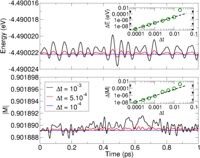
Figure 2: NVE SD–MD simulations of a block of 500 fcc cobalt atoms with periodic boundary conditions, with initial conditions corresponding to a temperature of 300 K. The graphs plot the energy per atom and the norm of the total magnetization $|{\rm\bm{M}}|$ for timesteps sizes of $10^{-3}$ ps (black), $5\cdot 10^{-4}$ ps (red), and $10^{-4}$ ps (blue). The two insets plot the mean relative absolute deviations of the energy $\Delta{E}$ and magnetization $\Delta|{\rm M}|$ according to Eq. 16 as a function of the timestep size $\Delta t$. The black dashed lines in the insets represent $\mathcal{O}\left(\Delta t^{2}\right)$ scaling behavior.

Because the system is closed, it cannot adiabatically exchange energy with a surrounding reservoir and both quantities are very well conserved. Typical spin dynamics simulations use a timestep of $\Delta t=10^{-4}$ ps. The current algorithm remains reasonably accurate up to a timestep size of $\Delta t=10^{-2}$ ps. This demonstrates the strong stability of the integration algorithm.

The influence of the timestep on the fluctuations in these quantities can be examined more precisely by calculating the mean relative absolute deviations averaged over the trajectory. For example, in the case of total energy per atom

$$\Delta{E}(\Delta t)=\frac{1}{N_{step}}\sum_{k=1}^{N_{step}}\left\lvert\frac{{E}_{k}(\Delta t)-\langle{E}\rangle(\Delta t)}{\langle{E}\rangle(\Delta t)}\right\rvert,$$ (16)

where $E_{k}$ is the total energy per atom at timestep $k$ and $\langle{E}\rangle$ is the time average of the total energy per atom.

The same formula can be applied to the norm of the total magnetization. The dependence of both of these quantities on the timestep size is shown in the two insets of Fig. 2. The deviations increase as $\mathcal{O}\left(\Delta t^{2}\right)$ . This behavior is consistent with the $\mathcal{O}\left(\Delta t^{3}\right)$ accuracy of the ST decomposition, which describes propagation over a single step. For $N$ consecutive steps, the accuracy of the decomposition algorithm is given by $\mathcal{O}\left(N\Delta t^{3}\right)$, with $N=t_{total}/\Delta t$. Thus, the accuracy for a fixed time interval is $\mathcal{O}\left(\Delta t^{2}\right)$, as seen in Fig. 2. For timestep size greater than $\Delta t=10^{-2}$ ps, the scaling law starts to break down, indicating the the limit of numerical stability is being approached.

4 Spin–lattice dynamics in a canonical ensemble (NVT)

Now we connect the spin–lattice system to an external energy reservoir and stabilize the exchanges of energy with a given thermostat. In MD, many approaches have been already explored [43, 44, 45] and we focus on a Langevin strategy [46]. This is a widely used thermostat for atomic systems as well as coarse-grained models, e.g. dissipative particle dynamics [47] (see [48] for a review). In the Langevin approach, both random forces and damping terms are used in accord with the fluctuation-dissipation theorem. However, the presence of damping terms will lead to a contraction of the phase space volume, producing non-Hamiltonian dynamics. Yet, even in these cases, it has been shown that if some phase-space related measures are not preserved, pathological situations can be observed, and lead to incorrect distributions [49].

4.1 Connecting spins to a random bath

Néel first [50] and Brown later [51] demonstrated that a sufficiently fine ferromagnetic particle consists of a single magnetic structure in which thermal agitation causes continual changes in the orientation of the moment. Such thermal fluctuations in the magnetization are well described by following the Langevin approach [9, 10, 52]. In this approach, the spin system is connected to a single thermal bath modeled by an infinite number of degrees of freedom. The properties of such bath are given by $\bm{\eta}$, a random vector, whose components follow a Gaussian probability law given by the first and second moment

$$\langle{\bm{\eta}}(t)\rangle = {\bm{0}}$$

$$\langle\eta_{\alpha}(t)\eta_{\beta}(t^{\prime})\rangle = 2D_{S}\delta_{\alpha\beta}\delta(t-t^{\prime})$$ (17)

where $\alpha$ and $\beta$ are the vector components.

In order to preserve the norm of each individual spin, this random fluctuation is added in a multiplicative manner to Eq. 1 via a random torque [53], that leads to the following stochastic Landau-Lifshitz-Gilbert equation :

$$\frac{d\bm{s}_{i}}{dt}=\frac{1}{\left(1+\lambda^{2}\right)}\left(\left(\bm{\omega}_{i}+\bm{\eta}\right)\times\bm{s}_{i}+\lambda\,\bm{s}_{i}\times\left(\bm{\omega}_{i}\times\bm{s}_{i}\right)\right).$$ (18)

From Eq. 18, one can derive a Fokker-Planck (FP) equation [52]. The resolution at equilibrium of the FP equation allows a fluctuation–dissipation relation to be derived that assigns a proportion of the amplitude of the noise $D_{S}$ to the given external thermostat $T$ [53], such that

$$D_{S}=\frac{2\pi\lambda k_{B}{T}}{\hbar},$$ (19)

with $k_{B}$ = the Boltzmann constant.

A subtle detail about stochastic differential equations is a proper choice of a stochastic prescription that allows an evaluation of the ill-defined random vector :

$$\bm{\mathcal{I}}(\Delta t)~{}=~{}\int_{t}^{t+\Delta t}\bm{\eta}(t^{\prime})\times\bm{s}_{i}(t^{\prime})dt^{\prime},$$ (20)

by defining a point within the interval $[t,t+\Delta t]$ at which this integral is approximated consistently. Numerous papers have discussed various choices of the prescription for stochastic magnetization dynamics performed with the stochastic LLG equation [52, 54, 55]. We use the mid–point Stratonovich approach that preserves the norm of individual spins and has time micro-reversibility.

4.2 Measuring lattice and spin temperatures

In non-equilibrium spin-lattice systems, it is convenient to use a single thermostat to control the flow of entropy production between the system and a thermal reservoir [56]. Such a thermostat has to be related to a microcanonical quantity defined in a statistical ensemble that measures the temperature. Because the temperature of an equilibrium system is calculated from the mean kinetic energy of its particles, the transient kinetic energy for spins is not an obvious quantity. An immediate consequence is how to measure the temperature $T_{S}$ that controls the thermostatting of the magnetic degrees of freedom [10].

At equilibrium, the instantaneous lattice temperature is usually defined as the kinetic temperature of the atoms:

$$T_{L}=\frac{2}{3\,N\,k_{B}}\sum_{i=1}^{N}\frac{|\bm{p}_{i}|^{2}}{2m_{i}}.$$ (21)

This expression of the kinetic temperature is known to rely on some approximations, such as the equivalence of ensembles and the ergodicity assumption [57]. Other dynamical approaches for measuring the temperature in Hamiltonian systems within a microcanonical ensemble have been derived, and proved to be accurate [58, 59]. However, we will assume that the kinetic expression given by eq. 21 is sufficient for the purpose of this work.

Transcripting Rugh’s the geometrical approach to spin systems [57], and when the thermodynamic limit is considered, Nurdin et al. [60] give a spin temperature as

$$T_{S}=\frac{\hbar}{2k_{B}}\frac{\sum_{i=1}^{N}|\bm{s}_{i}\times\bm{\omega_{i}}|^{2}}{\sum_{i=1}^{N}\bm{s}_{i}\cdot{\bm{\omega}}_{i}}$$ (22)

Another approach was later derived by Ma et al. [61]. Relying on the fluctuation-dissipation theorem, it gave an analog definition of the temperature of a spin ensemble.

In refs. [18, 19], the definition given by eq. 22 has proven to be efficient for the thermalization of the spin subsystem and its relaxation toward thermal equilibrium during spin–lattice simulations. Besides, this definition of $T_{S}$ has the same domain of validity as the kinetic temperature expressions for $T_{L}$ defined above. Thus, we chose to use the definition of the spin temperature defined by Nurdin et al..

4.3 Thermalizing the spin–lattice system

For the simulation of relaxation processes, the connecton of the lattice system to a thermal bath is also performed using the Langevin approach. Eq. 8 is replaced by Eq. 18, and a new random force and a damping term are added to Eq. 7. This yields the following equations that model stochastic magnetic molecular dynamics:

$$\frac{d\bm{r}_{i}}{dt} = \frac{\bm{p}_{i}}{m_{i}}$$ (23)

$$\frac{d\bm{p}_{i}}{dt} = \sum_{j,i\neq j}^{N}\left[-\frac{dV\left(r_{ij}\right)}{dr_{ij}}+\frac{dJ\left(r_{ij}\right)}{dr_{ij}}\bm{s}_{i}\cdot\bm{s}_{j}\right]\bm{e}_{ij}$$

$$-\frac{\gamma_{L}}{m_{i}}\bm{p}_{i}+\bm{f}(t)$$ (24)

$$\frac{d\bm{s}_{i}}{dt} = \frac{1}{\left(1+\lambda^{2}\right)}\left(\left(\bm{\omega}_{i}+\bm{\eta}(t)\right)\times\bm{s}_{i}+\lambda\,\bm{s}_{i}\times\left(\bm{\omega}_{i}\times\bm{s}_{i}\right)\right)$$ (25)

In Eq. 24, $\gamma_{L}$ is a damping parameter, and $\bm{f}$ its corresponding fluctuating force drawn from a Gaussian distribution with

$$\langle{\bm{f}}(t)\rangle = {\bm{0}}$$ (26)

$$\langle f_{\alpha}(t)f_{\beta}(t^{\prime})\rangle = D_{L}\,\delta_{\alpha\beta}\,\delta(t-t^{\prime})$$ (27)

where $\alpha$ and $\beta$ are coordinates, and $D_{L}$ is the amplitude of the random variables. $D_{L}$ can be parametrized according to the fluctuation–dissipation relation, and then depends on the temperature of the thermal bath coupled to the lattice, and on the damping coefficient $\gamma_{L}$ according to the Einstein relationship [39]. The probability distribution of the noise vector $\bm{\eta}$ follows Eqs. 17 and 19 respectively.

Extensions to more than two out-of-equilibrium dynamics (here referring to spin and lattice dynamics) are possible and several authors linked the damping coefficients to spin–electron and lattice–electron relaxation processes [62]. This allowed using the model presented above to simulate spin–lattice–electron relaxation processes that occur in ultrafast magnetic switching experiments.

However there are concerns about the choice of the noise correlation functions. In this study, we decided to remain within the framework of the Markov hypothesis, and focus on uncorrelated white-noise only. When the characteristic timescales of the dynamics reach values as small as those of the simulated relaxation processes, the Markov hypothesis may break down and a colored-noise, such as an Ornstein–Uhlenbeck process, becomes a better approximation of the exchange of causal information between the system and its reservoir. Recent studies have focused on evaluating the influence of such memory effects on the magnetization dynamics [63, 64, 65, 66], and suggest non-trivial magnetization dynamics beyond the second order cumulant of the spin variables. These points will be addressed in a separate study.

In order to evaluate the efficiency of the two-thermostat model presented here, two different simulations were performed. A cell of 500 cobalt atoms on an fcc lattice, coupled by three interactions (the magnetic exchange interaction, a spin-orbit coupling, and a mechanical EAM potential [31, 67]) is considered.

For the first simulation, a Langevin thermostat was applied only to the spins, according to Eq. 25. The simulation started from a fixed lattice equilibrium configuration, corresponding to $T_{L}=0$K and an initial spin configuration sampled from a $T_{S}=300$K magnetic equilibrium state.

The second simulation was exactly the opposite: the Langevin thermostat was applied only to the motion of the lattice atoms, according to Eq. 24. The simulation started in a configuration with all the spins aligned along their effective fields, which corresponds to $T_{S}=0$K, and with atom velocities sampled from a $T_{L}=300$K equilibrium lattice state. Fig. 3 plots the time evolution of $T_{L}$ and $T_{S}$ for the two simulations.

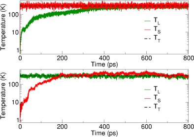
Figure 3: Measure of the spin T_S and lattice T_L temperatures during two NVT simulations of 500 cobalt atoms. For both graphs, the black dashed lines plot the target temperature T_T, and the green and red curves plot the lattice and spin temperatures, T_L and T_S, respectively. In the upper graph, the Langevin thermostat was applied to the spins only, according to Eq. 25, with a target T_T=300K, and the transverse magnetic damping set to $\lambda=0.01$. In the lower graph, the thermostat was applied only to the atomic motion, according to Eq. 24 with T_T=300K and a lattice damping parameter of $\gamma_{L}=10$ s^-1.

In each case, the thermostatted degrees of freedom stayed at the target temperature for the duration of the simulation. And the non-thermostated degrees of freedom relaxed from their initial temperature to the thermostatted temperature due to the spin–lattice coupling of the dynamics. In both cases the relaxation time was a few 100 ps, which is consistent with the spin–lattice coupling time shown in Fig. 1. This illustrates how proper choice of damping coefficients can produce physically correct responses for magnetic exchange, spin-orbit, and mechanical coupling interactions.

To better understand how the magnetic and mechanical energy couple to each other, a larger NVE simulation was performed with 1372 cobalt atoms initially on an fcc lattice. The initial spin configuration was random so that the spin system is in a paramagnetic state at a very high temperature. The atomic velocities (lattice temperature) were initialized to 200K. The potential energy of the atoms was initially at a minimum due to the perfect lattice configuration. As the simulation evolved energy re-partitioned between these 3 components (kinetic energy, potential energies of atoms and spins) but the total energy remained constant with no perceptible fluctuations (at this scale) as seen in the upper graph of Fig. 4. The lower graph of Fig. 4 plots the evovling spin and lattice temperatures, which equilibrated to the same value, indicating the efficacy of the spin–lattice coupling.

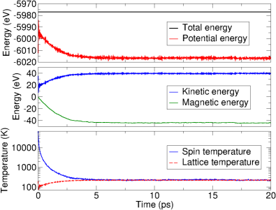
Figure 4: NVE simulation of a periodic block of 1372 cobalt atoms. Spin directions are initially random. Initial particle velocities were drawn from a Maxwell distribution at 200K. The upper graph plots 3 contributions to the total energy which remained constant: kinetic energy of the atoms and potential energies of the atoms and spins (magnetic energy). The lower graph plots the atomic (lattice) and spin temperatures, corresponding to Eqs. 21 and 22 respectively, which equilibrated to the same value.

5 Parallel implementation of the spin–lattice algorithm

5.1 Synchronous sub-lattice algoritm

To exploit the power of parallel processing, we developed a spatially-decomposed version of the serial SD–MD algorithm described in Section 3, analogous to that used for molecular dynamics simulations in LAMMPS. Like the serial algorithm, it is essential that the parallel algorithm accurately conserve energy and the norm of the total magnetization. As explained in Section 3, this requires that the spin propagation operators be applied in a manner that preserves symplecticity. This in turn requires that the magnetic force ${\bm{\omega}}_{i}$ acting on each spin ${\bm{s}}_{i}$ be calculated when each spin is updated. Due to short-range spin-spin interactions, the computation of this force depends on the spin orientations of the neighbors of atom $i$. In other words, before updating each spin, the current value of its neighboring spins must be known.

The parallel issue arises when two neighbor spins ${\bm{s}}_{i}$ and ${\bm{s}}_{j}$ (and their associated atoms) reside on different processors. How do we ensure that when the second spin is updated, it uses the previously updated value of the first spin? This clearly requires some inter-processor communication of spin information during the update operation, but the cost of the communication needs to be minimized to ensure an efficient algorithm. Likewise we must ensure two neighbor spins on different processors are not updated simultaneously (one of them with outdated information). Otherwise the accuracy of the integration scheme will be degraded..

Inspired by the lattice-dependent ST decomposition proposed by Krech et al. [68], Ma et al. [69] developed a multithreading algorithm for spin dynamics that partitions the single-spin evolution operators into groups whose member spins do not interact. This allows all spins in different groups to be updated concurrently by separate execution threads. The multi-threading implementation delivers good speedup on a single multicore CPU. As currently implemented, distributed-memory parallel execution is not supported, although the method could be extended to use spatial decomposition parallel algorithms. The biggest limitation of the method is the lack of generality. Partitioning into non-interacting groups is achieved using a lattice-coloring or checkerboarding scheme that can only be applied to perfectly regular lattices in which each spin interacts with a fixed stencil of interacting neighbor spins. Moreover, as the number of neighbors in the interaction stencil increases, the number of groups required to achieve a correct ST decomposition also increases, adding to the complexity of the algorithm.

We have implemented a different method called sectoring which is based on the synchronous sub-lattice algorithm [23, 70] used to achieve spatial parallelism in kinetic Monte Carlo simulations. In contrast to checkerboarding, sectoring is very general, requiring only that spin-spin interactions vanish beyond a finite cutoff distance. As long as this requirement is met, sectoring can be used for dynamic simulations of arbitrary systems of atomic spins, including perfectly regular lattices, thermally vibrating lattices, spatially disordered systems, and even systems undergoing diffusive dynamics in which the set of neighbors of each spin can change over time.

The sectoring method can be thought of as an extension to the spatial-decomposition MD algorithm used in LAMMPS and other MD codes, where the system is partitioned into subdomains, one per processor. Each processor owns and time-integrates the atoms in its subdomain. It also stores information about nearby ghost atoms, up to a cutoff distance away, which are owned by neighboring processors. This information is acquired by inter-processor communication, when needed.

The sectoring idea is to further divide each subdomain into smaller regions by bisecting the subdomain once in each physical dimension (4 sectors in 2d, 8 in 3d). If the spatial extent of all sectors in any dimension is larger than the interaction cutoff distance, then spins in the same sector on two different processors do not interact. The processors can thus concurrently update all the spins in one sector without the need to communicate spin information to/from other processors, while still adhering to the ST decomposition of Eq. 14. Formally, we can rewrite the ST decomposition as

$$e^{\hat{L}_{s}\frac{\Delta t}{2}}=\prod_{{k}=1}^{K}\left\{\prod_{{j}=1}^{N_{k}}e^{\hat{L}_{s_{j}}\frac{\Delta t}{4}}\right\}\prod_{{k}={K}}^{1}\left\{\prod_{{j=N_{k}}}^{1}e^{\hat{L}_{s_{j}}\frac{\Delta t}{4}}\right\}+\mathcal{O}\left(\Delta t^{3}\right),$$ (28)

where ${K}$ is the number of sectors, ${N_{k}}$ is the number of spins in sector ${k}$, and ${s_{j}}$ is the ${j}$th spin in the sector.

[width=0.5]figuresector

Figure 5: Schematic of the SD–MD sectoring algorithm for a two–dimensional spin–lattice model. The system is divided into four subdomains (bold squares), each owned by a different processor. Each subdomain is further divided into four sectors (numbered squares). Spins in sector 1 (shaded) for two different processors do not interact and can thus be updated concurrently without interprocessor communication.

Fig. 5 illustrates this idea for a two-dimensional system running on 4 processors, with each processor subdomain further divided into 4 sectors. Spins in sector 1 of a particular processor do not interact with spins in sector 1 of any other processor. Thus all the processors can update their sector 1 spins at the same time. After the sector 1 updates, new spin values must be communicated between processors before sector 2 spins can be updated.

Fig. 6 is a schematic of the necessary communication for the same 2d system. Each processor sends the current values of spins associated with the ghost atoms that border sector 1. The thickness of the border region is equal to the spin-spin interaction cutoff distance.

Note that Fig. 6 shows the minimal communication requirements. For simplicity and convenience, our current implementation makes use of standard communication functions in LAMMPS. All the ghost spins adjacent to the subdomain are updated, not only those adjacent to sector 1. This simplifies the implementation at the expense of a certain amount of unnecessary updating of spins that have not changed value. However, in either case, the cost of computation scales as $O((N/P)^{2/3})$, with $N$ the number of atoms and $P$ the number of MPI processes, differing only in the prefactor[71]. In applications where the communication cost is large relative to computation, extra overall performance could be achieved by limiting the interprocessor communication to only those sites adjacent to sector 1.

This pattern of communicating ghost spins then updating a sector is repeated four times, once for each sector (8 times in 3 dimensions). The entire process is then repeated in reverse sector order, at which point all of the spins have been updated by a half timestep, according to Eq. 28. Overall, spins in each sector are sequentially updated four times per timestep. To accurately integrate the spin dynamics, it is important that a fixed ordering of spins be used for all four updates. We achieve this by assigning atoms to sectors once at the start of the timestep based on their current positions.

[width=0.5]figurecomm

Figure 6: Schematic of the communication required before a processor can update spins in sector 1. This is a zoomed-in view of the bottom left portion of Fig. 5. The current values of all spins within the dashed square must be known before the processor updates spins in sector 1 (shaded). Most of these values are already known, because the spins are owned by the processor. But ghost spins in the blue regions are owned by neighboring processors, Those other processors must the send the current values to this processor. Similarly, this processor must send the current values of its spins in the red regions to neighboring processors. Once these communication operations have been completed, all the processors can concurrently advance their spins in sector 1.

5.2 Accuracy of the parallel algorithm

Note that by construction, the parallel algorithm faithfully reproduces the ST decomposition rule that each spin is updated using current information for all its neighbor spins. It differs from the serial algorithm only in the order in which the global set of spins are updated. This order will also differ depending on the number of processors used to run a simulation. Two simulations with different ordering will not evolve identically in a numerical sense, but they should be produce identical in a statistical sense, since both are “correct”. We tested this using the same fcc cobalt model used for testing the accuracy of the serial algorithm (Fig. 2). To allow for multiple processors, the size of the periodic simulation cell was increased from 17.7 Å (500 atoms) to 28.32 Å (2048 atoms). For a $2\times 2\times 2$ grid of 8 processors, the width of each sector is 7.08 Å, which is larger than the cutoff distance of 6.5 Å used by the EAM potential, and the one of 4.0 Å of the magnetic interactions. Starting with the same configuration initialized at 300 K, we ran serial and parallel NVE SD–MD simulations for 1 ps using a $10^{-4}$ps timestep. Fig. 7 plots the conservation of total energy and magnetization for the serial algorithm as well as the parallel algorithm running on 4 and 8 MPI processes.

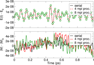
Figure 7: NVE SD–MD simulation of a block of 2048 fcc cobalt atoms using the sectoring parallel algorithm. The upper graph plots the energy E(t) minus the initial energy E₀ as a function of simulation time. The lower graph plots the norm of the total magnetization $|{\rm\bm{M}}|$ minus the initial value $|{\rm\bm{M}}|_{0}$. The black curves are for the serial algorithm, and the red and green curves (or dots for the upper graph) are for the parallel algorithm.

The upper graph of Fig. 7 shows the serial and parallel algorithms generate trajectories with tiny energy fluctuations that are indistinguishable from each other (the red and black curves overlay), especially relative to the size of the step-to-step variations in energy due to the numerical integration. The lower graph of Fig. 7 shows there there are tiny differences between the simulations in the total magnetization value at a particular timestep. This is expected, because the spins are updated in a different order in each simulation, leading to trajectories that diverge in a numerical sense. However the overall step-to-step variation in the magnetization is the same for all three simulations, indicating the parallel algorithm is generating a spin trajectory that is statistically equivalent to that of the serial simulation.

5.3 Scaling results

We now evaluate the scaling efficiency of the parallel spin–lattice algorithm as implemented in LAMMPS, for both strong and weak scaling. All simulations were performed on a cluster at Sandia consisting of dual-socket Intel Xeon E5-2695 (Broadwell) CPUs with 36 cores per node, and an Intel Omnipath interconnect. To ensure each processor owns the same number of spins, only 32 cores per node were used for each of the calculations, though this is not required for general runs.

Both strong and weak scaling tests were performed. In both cases, the parallel efficiency was evaluated by computing a normalized simulation rate (SR), defined as the number of atoms - steps per CPU second and per node:

$${\rm SR}=\frac{{\rm Steps}\times{\rm Atoms}}{{\rm Nodes}\times{\rm Seconds}}$$ (29)

and plotted as a function of the number of nodes.

Strong scaling was tested by increasing the number of nodes for a fixed number of atoms. Ideally, the computation time should be cut in half each time the number of nodes is doubled, so that SR should remain constant.

Each NVE SD–MD simulation combined a mechanical EAM potential with two magnetic interactions, the exchange energy and a Néel anisotropy (see A.1 and A.2 for more details). The magnetic potentials were parametrized according to Ref. [18]; the EAM potential is described in Ref. [67]. Two different problem sizes were run, the smaller with 256,000 (256K) atoms (a cubic box of $40^{3}$ fcc unit cells, 4 atoms/cell) and the larger with 2,048,000 (2M) atoms (2x larger in each dimension). The SR defined in Eq. 29 was averaged over a 50 timestep run. To assess the cost and efficiency of the SD–MD algorithm, the same simulations were run with only the EAM potential (no spin variables and without the sectoring algorithm). Fig. 8 shows the results.

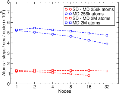
Figure 8: Strong-scaling performance of the parallel SD–MD algorithm (red) compared to standard MD (blue) for two fixed size problems. The smaller system (circles) has 256,000 atoms, the larger (squares) has 2,048,000 atoms. Perfect scaling would be horizontal lines.

Fig. 8 indicates the overall computational cost of including magnetic spin interactions, including the 8x increase in inter-processor communication to perform the sectoring algorithm, is about 4-5x that of a standard MD simulation with EAM potentials.

For perfect strong scaling, the SR should remain constant as the number of nodes increases. As the smaller system is run on more nodes, the relative cost of interprocessor communication grows as the atoms/node ratio shrinks, and the SR decreases slowly. The effect is less pronounced for the larger problem. Note that for the smaller problem, the maximum node count was 16 nodes ($32\times 16=512$ MPI tasks) to satisfy the requirement that the sector width be at least equal to the spin-spin interaction cutoff distance (4 Å). Also note that the higher computational cost of the SD–MD model results in somewhat better strong scaling efficiencies relative to standard MD.

Weak scaling was tested by increasing the size of the system as the number of nodes was increased, so that the number of atoms per node (and thus the size of each processor sub-domain) was held fixed.

The same magnetic and EAM interaction models were used as for the strong scaling runs. Two different sized systems with 32,000 (32K) (corresponding to 1,000 atoms per processor), and 256,000 (256K) atoms/node (corresponding to 8,000 atoms per processor) were simulated.

Fig. 9 shows the results for a number of nodes ranging from 1 to 64 (corresponding to 2,048 processes).

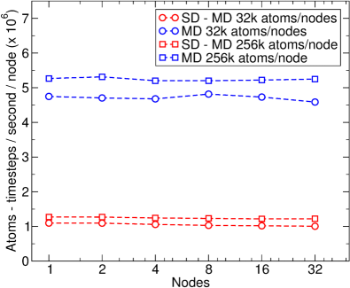
Figure 9: Performance of the parallel SD–MD algorithm compared to the standard MD algorithm for scaled size problems (weak scaling). In both cases, the interaction models are the same as that used in Fig. 8. The simulation rate (SR in Eq. 29) is plotted as a function of the number of nodes. SD–MD and MD results are colored red and blue, respectively. The smaller scaled systems (circles) consisted of 32,000 atoms/node and the larger scaled systems (squares) consisted of 256,000 atoms/node.

For ideal weak scaling, the value of SR should remain constant as the number of nodes increases, because the amount of work per process remains constant. Fig. 9 shows that SR indeed decreases very little, confirming the efficiency of our SD–MD algorithm. Also, we observe that our SD–MD algorithm is again approximately 4 to 5 times slower than the standard NVE MD calculation with LAMMPS, with the same EAM mechanical potential.

6 Conclusion

A parallel implementation of coupled magnetic and molecular dynamics was presented. This implementation of SD–MD is available as a new package in LAMMPS. It allows both coupled and uncoupled simulations to be performed, i.e. magnetic spins on a fixed lattice of atoms or on mobile atoms. Both the serial and parallel versions implement statistically equivalent symplectic Suzuki-Trotter decompositions of the spin propagation operators, differing only in the order they choose to update spins.

The accuracy of the serial version of the coupled algorithm was analyzed in both the microcanonical (NVE) and canonical (NVT) statistical ensembles. In the NVE case, care was taken to verify that both the total internal energy and the norm of the magnetization were conserved up to second order in the timestep size. For NVT simulations testing coupled spin–lattice relaxation, Langevin thermostats were applied to either the spin subsystem or the lattice subsystem.

A parallel implementation of the integration algorithm based on the sectoring or synchronous sublattice method was described in detail. The statistical equivalence of the parallel algorithm to the serial algorithm was verified by monitoring the conservation of total energy and the norm of the magnetization as the number of parallel processors varied. The parallel performance of the LAMMPS implementation was assessed, both for fixed size problems (strong scaling) and scaled size problems (weak scaling). In both cases, good performance was observed for all cases with more than 500 atoms per processor. Our new SD–MD algorithm with coupled magnetic spin and atomic lattice dynamics was shown to be only 4 to 5 times slower than an analogous NVE MD LAMMPS run treating only the motion of the atomic lattice.

This sectoring method has the advantage of being very general, working for both perfectly ordered particle configurations and disordered systems, so long as the width of each processor domain is at least twice the cutoff distance for the short-range spin-spin interactions.

Because the new methods were implemented within the open-source LAMMPS MD code, they are now available to the scientific community, enabling a wide variety of coupled spin–lattice simulations to be easily performed and tested in detail, as well as new models and algorithms to be implemented. Applications of this method to the simulation of magnetoelastic effects in magnetic alloys will be presented in subsequent publications.

Appendix A Definition of the spin Hamiltonian

In the equations of motion (eq.24), the mechanical force coming from the spins can be computed from the partial derivation of a spin Hamiltonian. This Hamiltonian represents the total energy of the magnetic systems. Its general form can be separated according to the following expression :

$$\mathcal{H}=\mathcal{H}_{z}+\mathcal{H}_{ex}+\mathcal{H}_{an}+\mathcal{H}_{N\acute{e}el}+\mathcal{H}_{dm}+\mathcal{H}_{me}+\mathcal{H}_{di},$$ (30)

with $\mathcal{H}_{z}$ and $\mathcal{H}_{ex}$ the Zeeman and the exchange interactions defined in Section 2, the magnetic anisotropy (2 terms), the Dzyaloshinskii-Moriya, the magneto-electric, and the dipolar interaction. The subsections of this appendix give a definition of these interactions.

A.1 Parametrization of the exchange interaction

Because of the celebrated Bohr-van Leuween theorem [72], the flow of permanent magnetic moments cannot be the origin of the magnetism found in actual materials and more surprisingly, magnetism is an inherently quantum mechanical effect. It is the interplay of electronic properties which appear unrelated to magnetism, the Pauli principle in combination with the Coulomb repulsion as well as the hopping of electrons that leads to an effective coupling between the magnetic moments in a solid [73]. This mechanism does not have a classical analogue and is responsible for both the volume of matter and ferromagnetism.

In SD-MD, an effective parametrization of this exchange interaction comes with two consequences : First, it is assuming that its intensity is rapidly decreasing with very few oscillations of its sign, so that a rigid cutoff radius $R_{c}$ can be safely introduced. For the computation of the exchange interaction with a given spin $i$, only spins $j$ such that $r_{ij}<R_{c}$ have to be taken into account. Second, the value of its intensity can be approximated by a simple continuous isotropic function ${J}\left(r_{ij}\right)$. For $3d$ atoms, this function is based on the Bethe–Slater curve [74, 75], and is parametrized via three coefficients, $\alpha$ in eV, $\delta$ in Å, and $\gamma$ a non-dimensional constant. One has :

$${J}\left(r_{ij}\right)=4\alpha\left(\frac{r_{ij}}{\delta}\right)^{2}\left(1-\gamma\left(\frac{r_{ij}}{\delta}\right)^{2}\right)e^{-\left(\frac{r_{ij}}{\delta}\right)^{2}}\Theta(R_{c}-r_{ij}),$$ (31)

with $\Theta(R_{c}-r_{ij})$ the Heaviside step function.

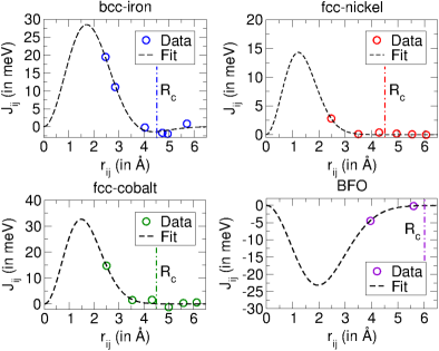
Figure 10: Examples of exchange curves for bcc-Fe in blue, fcc-Ni in red, fcc-Co in green, and bismuth ferrite oxide (BFO) in purple. The dotted line labeled R_c represents a cutoff radius taking into account the three first neighbor shells.

As examples, Fig. 10 plots the interpolation by the function presented in Eq. 31 of different exchange data. On one side, the three first sets are related to pure ferromagnetic metals such as Iron, Nickel and Cobalt, and come from ab initio calculations performed within the non-relativistic spin-polarized Green-function technique [76], in general agreement with scattering experiments. On the other side, the fourth set is for anti-ferromagnetic BiFeO₃ (BFO) and was measured by inelastic neutron scattering technique [77]. The values of the coefficients $\alpha$, $\gamma$ and $\delta$ to use for each of these four materials are gathered in table 1.

	$\alpha$ (meV)	$\gamma$	$\delta$ (Å)
Bcc-Fe	25.498	0.281	1.999
Fcc-Ni	9.73	$1.08\cdot 10^{-4}$	1.233
Fcc-Co	22.213	$8.08\cdot 10^{-6}$	1.485
BFO	-15.75	0	1.965

Table 1: Coefficients fitting the ab initio and experimental results (with the model presented in Eq. 31) for bcc-Fe, fcc-Ni, fcc-Co and bismuth ferrite oxide (BFO).

A.2 Spin orbit coupling

The spin-orbit coupling is of fundamental importance when SD-MD simulations are at stake. This is, for example, the case with magnetocrystalline anisotropy, or the Dzyaloshinskii-Moriya interaction [75]. Even if its non-relativistic origin corresponds to energies that are orders of magnitude lower than the exchange interaction, many technological application rely on effective interactions arising from that spin-orbit coupling [78].

Depending on the crystalline lattice of the material under study, different forms of local magnetic anisotropies can arise. A first simple phenomenological model accounting for the one-site magnetocrystalline anisotropy consists of shaping the angular dependence of the corresponding energy surface with spherical harmonics.

As an example, for uniaxial anisotropy, one has:

$$\mathcal{H}_{an}=-\sum_{{i}=1}^{N}K_{an}(\bm{r}_{i})\,\left(\bm{s}_{i}\cdot\bm{n}_{i}\right)^{2},$$ (32)

with $\bm{n}_{i}$ the direction of the anisotropy axis for the spin $i$, and $K_{an}(\bm{r}_{i})$ its anisotropic constant (in eV), which depends eventually to the position of the spin i. With this form of interaction, and depending on the sign of $K_{an}(\bm{r}_{i})$, the result can be either an easy axis or an easy plane for the magnetization (easy axis if $K_{an}(\bm{r}_{i})>0$, easy plane for $K_{an}(\bm{r}_{i})<0$).

However, in most magnetic crystals, the magnetocrystalline anisotropy takes more complex forms (like cubic anisotropy for example). Besides, this anisotropy model does not exhibit a clear dependence on the lattice parameters.

Another, more sophisticated model aimed at taking into account the magnetocrystalline anisotropy is the two-site non-local Néel anisotropy [34]. Limited to the pseudo-dipolar term only, one has:

$$\mathcal{H}_{N\acute{e}el} = -\sum_{{i,j=1,i\neq j}}^{N}g_{1}(r_{ij})\left(({\bm{e}}_{ij}\cdot{\bm{s}}_{i})({\bm{e}}_{ij}\cdot{\bm{s}}_{j})-\frac{1}{3}{\bm{s}}_{i}\cdot{\bm{s}}_{j}\right),$$

with $g_{1}(r)$ a fast decreasing function of $r$. Terms like $\sum_{{i,j=1,i\neq j}}^{N}g_{1}(r_{ij}){\bm{s}}_{i}\cdot{\bm{s}}_{j}$ can be viewed as special case of exchange interaction and can be omitted, by considering a well-suited redefinition of $J({r_{ij}})$. In our implementation, $g_{1}(r)$ was chosen to be the same function of three parameters as for the exchange interaction (see eq. 31).

It is also well known that the combination of the exchange interaction and the spin-orbit coupling can give rise to non-collinear spin states. First an object of theoretical work, this canted ferromagnetism (the ground state presents spins that are not perfectly aligned, but slightly tilted with one another) has since become a promising effect for many potential applications [79, 80].

The most common way to simulate this effect is to couple the exchange interaction (see Section. 2.1 and A.1) to another interaction, referred to as the anti–symmetric Dzyaloshinskii-Moriya interaction [81, 82]. This interaction takes the following form:

$$\mathcal{H}_{dm}=\sum_{{i,j}=1,i\neq j}^{N}\bm{D}(r_{ij})\cdot\left(\bm{s}_{i}\times\bm{s}_{j}\right),$$ (33)

with $\bm{D}(r_{ij})$ the Dzyaloshinskii-Moriya vector, which defines both the intensity (in eV) and the direction for the effect. In particular, the Dzyaloshinskii-Moriya interaction is known to be a key mechanism in the stabilization of magnetic skyrmions [83].

A.3 Magneto–electric interaction

In some materials, like BFO, magnetism coexists and interplays with dielectric permanent polarization at the atomic scale. According to Katsura et al. [84] and Mostovoy [85], the effects of this interplay can be taken into account within SD-MD via an anti–symmetric spin–spin effective interaction, as a particular case of the Dzyaloshinskii-Moriya vector, such as:

$$\mathcal{H}_{me}=\sum_{i,j=1,i\neq j}^{N}\left(\bm{E}\times\bm{e}_{ij}\right)\cdot\left(\bm{s}_{i}\times\bm{s}_{j}\right),$$ (34)

with $\bm{E}$ giving the direction and the intensity of a screened dielectric atomic polarization (in eV). This polarization can also be induced by an external electric field of sufficient intensity.

A.4 Dipolar interaction

With larger atomic systems, the long-range dipolar interaction is responsible for the stabilization of domain walls and the nucleation of magnetic domains. As such, it is often referred to as a demagnetizing field.

Its general non-local expression is

$$\mathcal{H}_{di}=-\frac{\mu_{0}\mu_{B}^{2}}{4\pi}\sum_{i,j=1,i\neq j}^{N}\frac{g_{i}g_{j}}{\bm{r}_{ij}^{3}}\left((\bm{s}_{i}\cdot\bm{e}_{ij})(\bm{s}_{j}\cdot\bm{e}_{ij})-\frac{1}{3}(\bm{s}_{i}\cdot\bm{s}_{i})\right),$$ (35)

with $g_{i}$ and $g_{j}$ the Landé factors for spins $i$ and $j$ respectively, $\bm{r}_{ij}=\bm{r}_{j}-\bm{r}_{i}$, and $\bm{e}_{ij}=\bm{r}_{ij}/|\bm{r}_{ij}|$.

Despite its simple formula, its computational cost is one of the main limiting factors for large magnetic simulations. Indeed, due to its long-range nature, the dipolar interaction does not have a finite cutoff distance, and therefore scales computationally as $N^{2}$, with $N$ the number of atoms in the system.

To compute the dipolar effective field and force, two solutions have been considered. The first one takes advantage of the properties of the Suzuki–Trotter decomposition to avoid computing the dipolar interaction at each timestep. In MD simulations, this solution is often considered when thermostats or barostats have very different characteristic time scales, and is referred to as the r-RESPA algorithm [86]. A second one relies on an assumption of periodicity in space to use the well known technique of Ewald sums [40]. For now, neither of these solutions are implemented for the SD-MD package in LAMMPS, but are being actively tested. Note that because the intensity of the dipolar interaction is usually much smaller than other considered magnetic interactions, in magnetic systems below the paramagnetic limit that are small enough to avoid the nucleation of domain walls, this effect can be safely omitted.

Appendix B Parametrization of a mechanical potential

In MD, the standard approach to simulate properties of metals is to consider a mechanical interaction between the magnetic atoms using a empirial many-body potential such as the embedded atom method (EAM) [87].

Dudarev et al followed this strategy and developed a very specific semi-empirical many-body interatomic potential suitable for large scale molecular dynamics simulations of magnetic $\alpha$-iron [36]. The functional form of the embedding portion of that potential is derived using a combination of the Stoner and the Ginzburg–Landau models, and reveals the spontaneous magnetization of atoms by a broken symmetry of the solutions of the Ginzburg–Landau model. Even if this strategy provides a link between magnetism and interatomic forces, the anisotropy effect through the spin-orbit coupling does not emerge naturally. This is not the strategy we have followed in this paper because we consider the magnitude of each atom’s magnetic moment to be fixed during the simulation. Only its direction changes over time. However, there is no conceptual difficulty with implementing the more detailed potential in LAMMPS.

Because EAM potentials are either fitted to experimental or ab initio data, the influence of the magnetic interactions is already silently included. In the framework of ab initio derived EAM potentials, this can be seen in the special case of collinear magnetism. Thus the standard approach is to effectively subtract the magnetic interactions from the mechanical potential, as :

$$\mathcal{H}_{mech}^{eff}(\bm{r}_{i})=\mathcal{H}_{mech}(\bm{r}_{i})-\mathcal{H}_{mag}^{ground}(\bm{r}_{i}),$$ (36)

with $\mathcal{H}_{mech}^{eff}(\bm{r}_{i})$ the mechanical potential that needs computing, $\mathcal{H}_{mech}(\bm{r}_{i})$ the EAM potential fitted before the magnetic energy subtraction, and $\mathcal{H}_{mag}^{ground}(\bm{r}_{i})$ the magnetic ground-state energy value. For example in a ferromagnet, because the exchange energy is by far the most intense value, the associated ground state is given by the following sum, with $j$ the neighboring atoms of the atom $i$:

$$\mathcal{H}_{mag}^{ground}(\bm{r}_{i})=\sum_{{j}=1}^{Neigh}{J}(r_{ij})\,|\bm{s}_{i}|\,|\bm{s}_{j}|.$$ (37)

Future work will study how the combination of both experimental and ab initio results can be used to derive better empirical magneto-mechanical potentials.

References

- Smith [2005] R. C. Smith, Smart Material Systems, Model Development, Frontiers in Applied Mathematics, SIAM, 2005.
- Rossi et al. [2005] E. Rossi, O. G. Heinonen, A. H. MacDonald, Dynamics of magnetization coupled to a thermal bath of elastic modes, Physical Review B 72 (2005).
- Beaurepaire et al. [1996] E. Beaurepaire, J.-C. Merle, A. Daunois, J.-Y. Bigot, Ultrafast spin dynamics in ferromagnetic nickel, Physical Review Letters 76 (1996) 4250.
- Qian and Vignale [2002] Z. Qian, G. Vignale, Dynamical exchange-correlation potentials for an electron liquid, Physical Review B 65 (2002) 235121.
- Restrepo and Windl [2012] O. D. Restrepo, W. Windl, Full First-Principles Theory of Spin Relaxation in Group-IV Materials, Physical Review Letters 109 (2012).
- Ozdemir Kart and Cagın [2010] S. Ozdemir Kart, T. Cagın, Elastic properties of Ni2mnga from first-principles calculations, Journal of Alloys and Compounds 508 (2010) 177–183.
- McQuarrie [1976] D. A. McQuarrie, Statistical Mechanics, HarperCollins Publishers, New York, 1976.
- Aharoni [1996] A. Aharoni, Introduction to the Theory of Ferromagnetism, number 93 in International series of monographs on physics, Oxford Science Publications, 1996.
- Antropov et al. [1995] V. P. Antropov, M. I. Katsnelson, M. Van Schilfgaarde, B. N. Harmon, Ab Initio Spin Dynamics in Magnets, Physical Review Letters 75 (1995) 729–732.
- Antropov et al. [1996] V. P. Antropov, M. I. Katsnelson, B. N. Harmon, M. Van Schilfgaarde, D. Kusnezov, Spin dynamics in magnets: Equation of motion and finite temperature effects, Physical Review B 54 (1996) 1019.
- Skubic et al. [2008] B. Skubic, J. Hellsvik, L. Nordström, O. Eriksson, A method for atomistic spin dynamics simulations: implementation and examples, Journal of Physics: Condensed Matter 20 (2008) 315203.
- Eriksson et al. [2017] O. Eriksson, A. Bergman, J. Hellsvik, L. Bergqvist, Atomistic spin dynamics: Foundations and applications, Oxford University Press, 2017.
- Radu et al. [2011] I. Radu, K. Vahaplar, C. Stamm, T. Kachel, N. Pontius, H. Dürr, T. Ostler, J. Barker, R. Evans, R. Chantrell, others, Transient ferromagnetic-like state mediating ultrafast reversal of antiferromagnetically coupled spins, Nature 472 (2011) 205.
- Dupé et al. [2014] B. Dupé, M. Hoffmann, C. Paillard, S. Heinze, Tailoring magnetic skyrmions in ultra-thin transition metal films, Nature communications 5 (2014) 4030.
- Tranchida et al. [2016] J. Tranchida, P. Thibaudeau, S. Nicolis, A functional calculus for the magnetization dynamics, arXiv preprint arXiv:1606.02137 (2016).
- Ma et al. [2008] P.-W. Ma, C. H. Woo, S. L. Dudarev, Large-scale simulation of the spin-lattice dynamics in ferromagnetic iron, Physical Review B 78 (2008) 024434.
- Ma et al. [2016] P.-W. Ma, S. L. Dudarev, C. H. Woo, SPILADY: A parallel CPU and GPU code for spin–lattice magnetic molecular dynamics simulations, Computer Physics Communications 207 (2016) 350–361.
- Beaujouan et al. [2012] D. Beaujouan, P. Thibaudeau, C. Barreteau, Anisotropic magnetic molecular dynamics of cobalt nanowires, Physical Review B 86 (2012) 174409.
- Perera et al. [2016] D. Perera, M. Eisenbach, D. M. Nicholson, G. M. Stocks, D. P. Landau, Reinventing atomistic magnetic simulations with spin-orbit coupling, Physical Review B 93 (2016) 060402.
- Perera et al. [2017] D. Perera, D. M. Nicholson, M. Eisenbach, G. M. Stocks, D. P. Landau, Collective dynamics in atomistic models with coupled translational and spin degrees of freedom, Physical Review B 95 (2017) 014431.
- Plimpton et al. [2007] S. Plimpton, P. Crozier, A. Thompson, LAMMPS-Large-scale Atomic/Molecular Massively Parallel Simulator, Sandia National Laboratories 18 (2007).
- Blanes et al. [2009] S. Blanes, F. Casas, J. A. Oteo, J. Ros, The Magnus expansion and some of its applications, Physics Reports 470 (2009) 151–238.
- Shim and Amar [2005] Y. Shim, J. G. Amar, Semirigorous synchronous sublattice algorithm for parallel kinetic Monte Carlo simulations of thin film growth, Physical Review B 71 (2005) 125432.
- Bacry [1962] H. Bacry, Thomas’s classical theory of spin, Il Nuovo Cimento 26 (1962) 1164–1172.
- Thomas [1926] L. H. Thomas, The Motion of the Spinning Electron, Nature 117 (1926) 514–514.
- Thomas [1927] L. Thomas, I. The kinematics of an electron with an axis, The London, Edinburgh, and Dublin Philosophical Magazine and Journal of Science 3 (1927) 1–22.
- Weiss [2012] U. Weiss, Quantum dissipative systems, World Scientific, New Jersey, NJ, 4. ed edition, 2012.
- Wieser [2015] R. Wieser, Description of a dissipative quantum spin dynamics with a Landau-Lifshitz/Gilbert like damping and complete derivation of the classical Landau-Lifshitz equation, The European Physical Journal B 88 (2015).
- Gilbert [2004] T. L. Gilbert, A phenomenological theory of damping in ferromagnetic materials, IEEE Transactions on Magnetics 40 (2004) 3443–3449.
- Ebert et al. [2011] H. Ebert, S. Mankovsky, D. Ködderitzsch, P. J. Kelly, Ab Initio Calculation of the Gilbert Damping Parameter via the Linear Response Formalism, Physical Review Letters 107 (2011).
- Thibaudeau and Beaujouan [2012] P. Thibaudeau, D. Beaujouan, Thermostatting the atomic spin dynamics from controlled demons, Physica A: Statistical Mechanics and its Applications 391 (2012) 1963–1971.
- Kittel and Fong [1987] C. Kittel, C.-y. Fong, Quantum theory of solids: includes solutions appendix, prepared by C.Y. Fong, Wiley, New York, 2., rev. print edition, 1987.
- Victora and MacLaren [1993] R. H. Victora, J. M. MacLaren, Theory of magnetic interface anisotropy, Physical Review B 47 (1993) 11583–11586.
- Néel [1954] L. Néel, L’approche à la saturation de la magnétostriction, Journal de Physique et le Radium 15 (1954) 376–378.
- Bruno [1988] P. Bruno, Magnetic surface anisotropy of cobalt and surface roughness effects within Neel’s model, Journal of Physics F: Metal Physics 18 (1988) 1291–1298.
- Dudarev and Derlet [2005] S. Dudarev, P. Derlet, A ‘magnetic’interatomic potential for molecular dynamics simulations, Journal of Physics: Condensed Matter 17 (2005) 7097.
- Thibaudeau and Gale [2008] P. Thibaudeau, J. Gale, An embedded-atom method model for liquid Co, Nb, Zr and supercooled binary alloys, arXiv preprint arXiv:0809.0198 (2008).
- Yang and Hirschfelder [1980] K.-H. Yang, J. O. Hirschfelder, Generalizations of classical Poisson brackets to include spin, Physical Review A 22 (1980) 1814.
- Tuckerman [2010] M. Tuckerman, Statistical mechanics: theory and molecular simulation, Oxford University Press, 2010.
- Frenkel and Smit [2002] D. Frenkel, B. Smit, Understanding molecular simulation: from algorithms to applications, Academic Press, San Diego, 2 edition, 2002.
- Omelyan et al. [2001] I. Omelyan, I. Mryglod, R. Folk, Algorithm for molecular dynamics simulations of spin liquids, Physical Review Letters 86 (2001) 898.
- Dullweber et al. [1997] A. Dullweber, B. Leimkuhler, R. McLachlan, Symplectic splitting methods for rigid body molecular dynamics, The Journal of Chemical Physics 107 (1997) 5840–5851.
- Andersen [1980] H. C. Andersen, Molecular dynamics simulations at constant pressure and/or temperature, The Journal of Chemical Physics 72 (1980) 2384–2393.
- Nosé [1984] S. Nosé, A unified formulation of the constant temperature molecular dynamics methods, The Journal of Chemical Physics 81 (1984) 511–519.
- Hoover [1985] W. G. Hoover, Canonical dynamics: Equilibrium phase-space distributions, Physical Review A 31 (1985) 1695–1697.
- Feller et al. [1995] S. E. Feller, Y. Zhang, R. W. Pastor, B. R. Brooks, Constant pressure molecular dynamics simulation: The Langevin piston method, The Journal of Chemical Physics 103 (1995) 4613–4621.
- Hoogerbrugge and Koelman [1992] P. J. Hoogerbrugge, J. M. V. A. Koelman, Simulating Microscopic Hydrodynamic Phenomena with Dissipative Particle Dynamics, Europhysics Letters 19 (1992) 155–160.
- Groot and Warren [1997] R. D. Groot, P. B. Warren, Dissipative particle dynamics: Bridging the gap between atomistic and mesoscopic simulation, The Journal of Chemical Physics 107 (1997) 4423–4435.
- Tuckerman et al. [2001] M. E. Tuckerman, Y. Liu, G. Ciccotti, G. J. Martyna, Non-Hamiltonian molecular dynamics: Generalizing Hamiltonian phase space principles to non-Hamiltonian systems, The Journal of Chemical Physics 115 (2001) 1678–1702.
- Néel [1949] L. Néel, Influence des fluctuations thermiques sur l’aimantation de grains ferromagnétiques très fins, Compte Rendus de l’Académie des Sciences 228 (1949) 664.
- Brown [1963] W. F. Brown, Thermal Fluctuations of a Single-Domain Particle, Physical Review 130 (1963) 1677–1686.
- García-Palacios and Lázaro [1998] J. L. García-Palacios, F. J. Lázaro, Langevin-dynamics study of the dynamical properties of small magnetic particles, Physical Review B 58 (1998) 14937.
- Mayergoyz et al. [2009] I. D. Mayergoyz, G. Bertotti, C. Serpico, Nonlinear magnetization dynamics in nanosystems, Elsevier, 2009.
- d’Aquino et al. [2006] M. d’Aquino, C. Serpico, G. Coppola, I. Mayergoyz, G. Bertotti, Midpoint numerical technique for stochastic Landau-Lifshitz-Gilbert dynamics, Journal of Applied Physics 99 (2006) 08B905.
- Aron et al. [2014] C. Aron, D. G. Barci, L. F. Cugliandolo, Z. G. Arenas, G. S. Lozano, Magnetization dynamics: path-integral formalism for the stochastic Landau–Lifshitz–Gilbert equation, Journal of Statistical Mechanics: Theory and Experiment 2014 (2014) P09008.
- Rapaport [2004] D. C. Rapaport, The Art of Molecular Dynamics Simulation, Cambridge University Press, 2nd edition, 2004.
- Rugh [1997] H. H. Rugh, Dynamical approach to temperature, Physical Review Letters 78 (1997) 772.
- Rugh [1998] H. H. Rugh, A geometric, dynamical approach to thermodynamics, Journal of Physics A: Mathematical and General 31 (1998) 7761.
- Jepps et al. [2000] O. G. Jepps, G. Ayton, D. J. Evans, Microscopic expressions for the thermodynamic temperature, Physical Review E 62 (2000) 4757–4763.
- Nurdin and Schotte [2000] W. B. Nurdin, K.-D. Schotte, Dynamical temperature for spin systems, Physical Review E 61 (2000) 3579.
- Ma et al. [2010] P.-W. Ma, S. L. Dudarev, A. A. Semenov, C. H. Woo, Temperature for a dynamic spin ensemble, Physical Review E 82 (2010).
- Ma et al. [2012] P.-W. Ma, S. Dudarev, C. Woo, Spin-lattice-electron dynamics simulations of magnetic materials, Physical Review B 85 (2012) 184301.
- Atxitia et al. [2009] U. Atxitia, O. Chubykalo-Fesenko, R. W. Chantrell, U. Nowak, A. Rebei, Ultrafast Spin Dynamics: The Effect of Colored Noise, Physical Review Letters 102 (2009).
- Bose and Trimper [2010] T. Bose, S. Trimper, Correlation effects in the stochastic Landau-Lifshitz-Gilbert equation, Physical Review B 81 (2010).
- Tranchida et al. [2016a] J. Tranchida, P. Thibaudeau, S. Nicolis, Closing the hierarchy for non-Markovian magnetization dynamics, Physica B: Condensed Matter 486 (2016a) 57–59.
- Tranchida et al. [2016b] J. Tranchida, P. Thibaudeau, S. Nicolis, Colored-noise magnetization dynamics: from weakly to strongly correlated noise, IEEE Transactions on Magnetics 52 (2016b) 1300504.
- Pun and Mishin [2012] G. P. Pun, Y. Mishin, Embedded-atom potential for hcp and fcc cobalt, Physical Review B 86 (2012) 134116.
- Krech et al. [1998] M. Krech, A. Bunker, D. Landau, Fast spin dynamics algorithms for classical spin systems, Computer Physics Communications 111 (1998) 1–13.
- Ma and Woo [2009] P.-W. Ma, C. Woo, Parallel algorithm for spin and spin-lattice dynamics simulations, Physical Review E 79 (2009) 046703.
- Plimpton et al. [2009] S. Plimpton, C. Battaile, M. Chandross, L. Holm, A. Thompson, V. Tikare, G. Wagner, E. Webb, X. Zhou, C. G. Cardona, others, Crossing the mesoscale no-man’s land via parallel kinetic Monte Carlo, Technical Report SAND2009-6226, Sandia National Laboratories, 2009.
- Plimpton [1995] S. Plimpton, Fast parallel algorithms for short-range molecular dynamics, Journal of computational physics 117 (1995) 1–19.
- Van Leeuwen [1921] H.-J. Van Leeuwen, Problèmes de la théorie électronique du magnétisme, Journal de Physique et le Radium 2 (1921) 361–377.
- Duck and Sudarshan [1998] I. Duck, E. C. G. Sudarshan, Pauli and the Spin-Statistics Theorem, World Scientific, 1998.
- Kaneyoshi [1992] T. Kaneyoshi, Introduction to amorphous magnets, World Scientific, Singapore, 1992.
- Yosida [1996] K. Yosida, Theory of magnetism, number 122 in Springer series in solid-state sciences, Springer, Berlin ; New York, 1996.
- Pajda et al. [2001] M. Pajda, J. Kudrnovsky, I. Turek, V. Drchal, P. Bruno, Ab initio calculations of exchange interactions, spin-wave stiffness constants, and Curie temperatures of Fe, Co, and Ni, Physical Review B 64 (2001) 174402.
- Jeong et al. [2012] J. Jeong, E. Goremychkin, T. Guidi, K. Nakajima, G. S. Jeon, S.-A. Kim, S. Furukawa, Y. B. Kim, S. Lee, V. Kiryukhin, others, Spin Wave Measurements over the Full Brillouin Zone of Multiferroic BiFeO3, Physical Review Letters 108 (2012) 077202.
- Skomski [2008] R. Skomski, Simple models of magnetism, Oxford graduate texts, Oxford University Press, Oxford ; New York, 2008.
- Muhlbauer et al. [2009] S. Muhlbauer, B. Binz, F. Jonietz, C. Pfleiderer, A. Rosch, A. Neubauer, R. Georgii, P. Boni, Skyrmion Lattice in a Chiral Magnet, Science 323 (2009) 915–919.
- Fert et al. [2013] A. Fert, V. Cros, J. Sampaio, Skyrmions on the track, Nature Nanotechnology 8 (2013) 152–156.
- Dzyaloshinsky [1958] I. Dzyaloshinsky, A thermodynamic theory of “weak” ferromagnetism of antiferromagnetics, Journal of Physics and Chemistry of Solids 4 (1958) 241–255.
- Moriya [1960] T. Moriya, Anisotropic Superexchange Interaction and Weak Ferromagnetism, Physical Review 120 (1960) 91–98.
- Rohart and Thiaville [2013] S. Rohart, A. Thiaville, Skyrmion confinement in ultrathin film nanostructures in the presence of Dzyaloshinskii-Moriya interaction, Physical Review B 88 (2013).
- Katsura et al. [2005] H. Katsura, N. Nagaosa, A. V. Balatsky, Spin current and magnetoelectric effect in noncollinear magnets, Physical Review Letters 95 (2005) 057205.
- Mostovoy [2006] M. Mostovoy, Ferroelectricity in spiral magnets, Physical Review Letters 96 (2006) 067601.
- Tuckerman et al. [1992] M. Tuckerman, B. J. Berne, G. J. Martyna, Reversible multiple time scale molecular dynamics, The Journal of Chemical Physics 97 (1992) 1990–2001.
- Daw et al. [1993] M. S. Daw, S. M. Foiles, M. I. Baskes, The embedded-atom method: a review of theory and applications, Materials Science Reports 9 (1993) 251–310.