One-dimensional reduction of viscous jets. II. Applications

Abstract

In a companion paper [Pitrou, Phys. Rev. E 97, 043115 (2018)], a formalism allowing to describe viscous fibers as one-dimensional objects was developed. We apply it to the special case of a viscous fluid torus. This allows to highlight the differences with the basic viscous string model and with its viscous rod model extension. In particular, an elliptic deformation of the torus section appears because of surface tension effects, and this cannot be described by viscous string nor viscous rod models. Furthermore, we study the Rayleigh-Plateau instability for periodic deformations around the perfect torus, and we show that the instability is not sufficient to lead to the torus breakup in several droplets before it collapses to a single spherical drop. Conversely, a rotating torus is dynamically attracted toward a stationary solution, around which the instability can develop freely and split the torus in multiple droplets.

I Introduction

In our companion article Pitrou (2018), we developed a formalism to describe a viscous fiber as a one-dimensional object with an internal structure. Given the numerical complexity for solving the full set of fluid dynamics equations, taking into account junction conditions at the fiber side for the stress tensor, this description allows for a simpler route for the numerical resolution of viscous fiber dynamics. It is based on an expansion in the slenderness parameter $\epsilon_{R}\equiv{R}/L$, where ${R}$ is the radius of the fiber and $L$ is the scale associated with typical velocity gradients. At lowest order in this expansion, the description is exactly the same as a viscous string, with no internal resistance to bending nor twisting, and the fiber is only subject to tangential forces from stretching. However, at the next to leading order, which is ${\cal O}(\epsilon_{R}^{2})$ smaller, this description departs from the rod model developed in Refs. Arne et al. (2009); Ribe (2004); Ribe et al. (2006), which is another theoretical refinement of the viscous string model. The goal of this article is to emphasize the differences between these two formalisms, considering a torus of viscous fluid that shrinks due to the effect of surface tension. After summarizing the formalism in § II, we show in § III that the shrinking paces between our model and the rod model are slightly different, and we also emphasize the importance of the elliptic deformation of the torus section to obtain a coherent description. In § IV we exhibit the differences in the Rayleigh-Plateau instability, when considering the dispersion relation of periodic and linear deformations. We also solve numerically for the dynamical evolution of these linear perturbations. Finally, we revisit in § V the torus dynamics and the Rayleigh-Plateau instability for an initially rotating torus.

II One-dimensional description

In the next section, we briefly review the main features of our one-dimensional model for viscous fibers which is built in Ref. Pitrou (2018). We then emphasize the differences with the rod model in § II.2.

II.1 Summary of our formalism

At each time $t$, a viscous fiber is described as a one-dimensional object through the trajectory ${\bm{R}}(s,t)$ of its central line, where $s$ is a length parameter along this central line (see Fig. 1 of Ref. Pitrou (2018) for an illustration). The unit tangent vector to this central line is

$${\bm{T}}\equiv\partial_{s}{\bm{R}}\,$$ (1)

and the velocity of the central line is

$${\bm{U}}\equiv\partial_{t}{\bm{R}}\,.$$ (2)

Curvature of the central line at a given time is defined as

$${\bm{\kappa}}\equiv{\bm{T}}\times\partial_{s}{\bm{T}}\,.$$ (3)

A fiber section labeled by a given $s$ is made of points in the viscous fluid which lie in a plane containing ${\bm{R}}(s)$ and normal to ${\bm{T}}(s)$. For each section we form an orthonormal basis ${\bm{d}}_{\underline{i}}\equiv({\bm{d}}_{\underline{1}},{\bm{d}}_{\underline{2}},{\bm{d}}_{\underline{3}}={\bm{T}})$, and by construction the ${\bm{d}}_{\underline{a}},\,a=1,2$, are tangent to the section. Any vector ${\bm{X}}$ (e.g. the fluid velocity) can be split into longitudinal components (along ${\bm{T}}$) and sectional components (along the ${\bm{d}}_{\underline{a}}$) as

$${\bm{X}}=P_{\perp}({\bm{X}})+\overline{X}{\bm{T}}\,,\qquad P_{\perp}({\bm{X}})\equiv X^{a}{\bm{d}}_{\underline{a}}\,.$$ (4)

We also introduce the general notation

$$\widetilde{{\bm{X}}}\equiv{\bm{T}}\times{\bm{X}}\,,$$ (5)

and in particular $\widetilde{{\bm{\kappa}}}$ is a vector which points toward the exterior of the central line curvature.

The rotation rate of the frame is defined as

$$\partial_{t}{\bm{d}}_{\underline{i}}={\bm{\omega}}\times{\bm{d}}_{\underline{i}}\,.$$ (6)

From these definitions, one infers the constraints

$$(\partial_{s}{\bm{U}})\cdot{\bm{T}}&=0\,,\\ P_{\perp}({\bm{\omega}})={\bm{T}}\times\partial_{s}{\bm{U}}=\partial_{s}\widetilde{{\bm{U}}}+{\bm{\kappa}}\overline{U}\,.$$ (7)

The velocity of the fluid ${\bm{{\cal V}}}$ on the central line is decomposed into the velocity of the central line ${\bm{U}}$ and the velocity with respect to the central line ${\bm{V}}$, that is as

$${\bm{{\cal V}}}={\bm{U}}+{\bm{V}}\,.$$ (8)

In order to obtain a one-dimensional description for the viscous fiber, we expand in multipoles the variation in each section of the fluid velocity outside the central line. Several constraints from the boundary junction condition (which take into account surface tension effects) and from the Navier-Stokes equation, allow to express all of these multipoles in functions of $v$ and ${\dot{\phi}}$, which are, respectively, the longitudinal part of ${\bm{V}}$ [that is, $v\equiv\overline{V}$ using notation (4)] and the solid rotation rate of the fluid around the central line axis ${\bm{T}}$. Eventually, the description is reduced to the dynamics of these two quantities in addition to the central line motion found from the evolution of ${\bm{U}}$, combined with the evolution of the section shape which is allowed to depart from strict circularity.

In this procedure, there is a natural expansion in $\epsilon_{R}$. For instance, terms of the type $\kappa^{a}\kappa_{a}{R}^{2}$, where ${R}$ is the fiber radius, are of order ${\cal O}(\epsilon_{R}^{2})$. Keeping only the lowest order terms amounts to considering the viscous string model. However, our model for curved fibers in Ref. Pitrou (2018) consists in including the first corrections that are ${\cal O}(\epsilon_{R}^{2})$. In particular, when including these higher order effects, the shape of the sections cannot simply be described by the radius ${R}$ as it deforms. One must also account for an elliptic deformation, whose dynamics is found from the boundary condition.

II.2 The rod model

The rod model was used in steady or stationary situations in Refs. Ribe (2004); Ribe et al. (2006); Arne et al. (2009, 2015); Marheineke and Wegener (2007, 2009), but its formulation is general and can account for time dependence. It is based on three balance equations, namely, the matter balance equation, the momentum balance equation, and the angular momentum balance equation. We gathered the rod model equations and a discussion on their shortcomings in §  VII.G.4 of Ref. Pitrou (2018). To summarize, for the rod model one assumes that fiber sections remain i) circular, ii) orthogonal to the fiber central line, and iii) that the fluid velocity on the central line is such that the fluid particle on the central line stays on the central line [$P_{\perp}({\bm{V}})=0$].

• i) Assuming circular shapes is necessary to obtain meaningful momentum and angular momentum balance equations in the rod model. However we find that the an elliptic deformation is necessarily generated from fiber curvature as an ${\cal O}(\epsilon_{R}^{2})$ effect. Note that a first attempt of describing elliptic sections, but restricted to straight fibers, was performed independently in Ref. Bechtel et al. (1988).

• ii) For the fiber section to remain orthogonal to the central line, it requires that the solid rotation rate of the section is equal to the rotation rate of the fluid on central line at lowest order (see § VII.B.4 of Ref. Pitrou (2018)). Hence, the angular momentum balance cannot be an equation which determines the solid rotation of sections since it is determined already by the momentum balance equation. Instead, the sectional viscous forces $P_{\perp}({\bm{F}})$ which lead to a net torque ${\bm{T}}\times{\bm{F}}$ per unit of fiber length are constrained in the rod model by the angular momentum balance so as to enforce this property. Since the momentum of inertia of a fiber section scales as ${R}^{4}$ and sectional forces scale as ${R}^{2}$, we deduce that adding sectional forces to the momentum balance equation amounts to including order $\epsilon_{R}^{2}$ terms, which are otherwise absent in the lowest order string model.

• iii) We showed in § IV.I of Ref. Pitrou (2018) that to ensure that the central line remains on the section center, defined as the position for which there is no dipole in the shape deformation, the fluid velocity on the central line ($P_{\perp}({\bm{{\cal V}}})$) must be slightly different from the velocity of the central line ($P_{\perp}({\bm{U}})$), that is the difference which is $P_{\perp}({\bm{V}})$ does not vanish but is instead of order $\epsilon_{R}^{2}$. This was clearly identified in Ribe et al. (2006) but ignored precisely on the grounds that it was expected to be an order $\epsilon_{R}^{2}$ corrections. However, since the inclusion of sectional forces, which is the main difference between a rod model and a string model, is also a correction of order $\epsilon_{R}^{2}$, we found that it is formally inconsistent to choose one correction and discard another one, if they are formally of the same order.

III Dynamics of a shrinking torus

III.1 Adapted coordinates and variables

In order to highlight some differences between our formalism and the rod model, we study the special case of a viscous torus surrounded by vacuum. The case of a torus surrounded by a highly viscous fluid has been studied analytically in Ref. Bowick and Yao (2011) by considering the approximate Stokes flow equation.

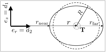
Figure 1: Notation in the plane of constant $\theta$.

There are natural cylindric coordinates $(r,\theta,z)$ associated with the torus with a basis of unit vectors ${\bm{e}}_{r},{\bm{e}}_{\theta},{\bm{e}}_{z}$ (see Fig. 1 for an illustration of the notation). Due to its high degree of symmetries, no quantity can depend on $\theta$, and if the fiber central line is in the plane $z=0$ it remains so. At any time, the fiber central line is entirely characterized by the radial distance $r(t)$, hence all quantities can only depend on $t$. In particular, torus sections cannot mix and there can be no sectional viscous forces. This implies that the viscous rod model matches exactly the viscous string model. Hence this system is of particular academic interest because on the contrary our model differs from the string model.

The orthonormal basis associated with the fiber coordinates is given by

$${\bm{d}}_{\underline{1}}\equiv{\bm{e}}_{z}\,,\quad{\bm{d}}_{\underline{2}}\equiv{\bm{e}}_{r}\,,\quad{\bm{T}}\equiv{\bm{e}}_{\theta}\,.$$ (9)

Starting from a reference angle, the relation between the polar angle $\theta$ and the affine parameter $s$ is simply

$$s=r\theta\,.$$ (10)

The fiber curvature has only one component $\kappa$ which is

$${\bm{\kappa}}=\kappa{\bm{e}}_{z}\,,\qquad{\bm{{\widetilde{\kappa}}}}=\kappa{\bm{e}}_{r}\,,\qquad\kappa\equiv\frac{1}{r}\,.$$ (11)

From the symmetries, the section ellipticity (see § IV.D of Ref. Pitrou (2018) for definitions) is necessarily fully specified by one polarization ${\cal E}$, and it is of the form

$${\cal R}^{ab}\equiv{\cal E}(e_{z}^{\,\,a}e_{z}^{\,\,b}-e_{r}^{\,\,a}e_{r}^{\,\,b})\,.$$ (12)

The central line sectional velocity is necessarily oriented radially. Hence we define

$$U^{a}\equiv U^{r}e_{r}^{\,a}\,.$$ (13)

As for the fiber longitudinal velocity $\bar{U}$, it is not vanishing because the geometric point of constant affine coordinate $s$ has a longitudinal motion due to the shrinking of the torus. Its value is determined by the structure relation (7) which implies

$$\partial_{s}\bar{U}=-{\bm{U}}\cdot{\bm{{\widetilde{\kappa}}}}=-U^{a}{\widetilde{\kappa}}_{a}=-\frac{U^{r}}{r}\,.$$ (14)

Since $U^{r}$ does not depend on $s$, we find

$$\bar{U}=-\frac{sU^{r}}{r}\,.$$ (15)

However, the total fluid tangential velocity on the central line is

$$\overline{\cal V}=\bar{U}+v\,,$$ (16)

and from the symmetries of the problem this quantity does not depend on $s$. If furthermore there is no initial rotation around the $z$ axis and the fluid falls radially, then $\overline{\cal V}=0$. We assume in this section that this is the case and we postpone the case $\overline{\cal V}\neq 0$ to § V.

One would naively expect that rotation of the fiber central line ${\bm{\omega}}$ should vanish due to the symmetries of the problem. However, it is defined as the rotation of the orthonormal basis for a geometric point of constant affine coordinate $s$, and it is instead obtained from the structure relation (7) which implies

$${\bm{\omega}}={\bm{\kappa}}\bar{U}\,.$$ (17)

Finally, the evolution of the radius ${R}$ satisfies

$$\frac{\partial_{t}{R}}{{R}}=-\frac{1}{2}\partial_{s}v=-\frac{U^{r}}{2r}=-\frac{\dot{r}}{2r}\,.$$ (18)

This is valid even when including corrections of order $\epsilon_{R}^{2}$, and it is an obvious consequence of volume conservation, which for a torus is $(2\pi r)\times(\pi{R}^{2})$. Hence, one can directly use its first integral which reads as

$$R=R_{i}\sqrt{\frac{r_{i}}{r}}\,.$$ (19)

Finally, let us define an aspect ratio parameter by

$$\epsilon_{i}=\frac{R_{i}}{r_{i}}\,,$$ (20)

which characterizes the initial shape of the torus.

III.2 Governing equations

From the dynamical equations gathered in § VII.B.9 of Ref. Pitrou (2018) for the lowest order string model and § VII.C.7 for the ${\cal O}(\epsilon_{R}^{2})$ corrections, we finally find

$$\ddot{r}=\partial_{t}U^{r}&=-\frac{{\nu}\kappa}{{R}}\left[1+\frac{7}{8}(\kappa{R})^{2}\right]\\ -3{\mu}\kappa^{2}U^{r}\left[1+\frac{11}{16}(\kappa{R})^{2}\right]\\ -\frac{21}{16}\kappa^{3}{R}^{2}(U^{r})^{2}+\overline{\cal V}^{2}\kappa\left[1+\tfrac{1}{2}(\kappa{R})^{2}\right]\,,\\ \frac{{\rm d}({\cal E}{R}^{2})}{{\rm d}t}=-\frac{{\nu}}{{R}{\mu}}\left[{\cal E}{R}^{2}+\frac{(\kappa{R})^{2}}{6}\right]\\ -\frac{7}{16}\kappa(\kappa{R})^{2}U^{r}-\frac{1}{12{\mu}}(\overline{\cal V}\kappa{R})^{2}\,.$$ (21)

Since we assumed that the fluid is incompressible, we chose a unit mass density $\rho$ so that the viscosity ${\mu}$ and surface tension ${\nu}$ stand in fact for ${\mu}/\rho$ and ${\nu}/\rho$. The first line of Eq. (21) is the radial force from surface tension which tends to shrink the torus, with its lowest order form and its first correction $\propto(\kappa{R})^{2}$. The second line corresponds to viscous friction, similarly given with the lowest order and its correction $\propto(\kappa{R})^{2}$. The first term in the last line is a convective effect and the last term vanishes if the torus is not rotating initially (see § V) as it corresponds to inertial forces. Eq. (21) rules the dynamical evolution of the elliptic deformation. Its last term vanishes if the fluid is not rotating as it corresponds to tidal inertial forces. In particular, when considered in the limit of vanishing viscosity, Eq. (21) amounts to the constraint

$${\cal E}{R}^{2}\simeq-\frac{(\kappa{R})^{2}}{6}\,.$$ (22)

It corresponds to the condition for which the quadrupole of extrinsic curvature [Eq. (7.34c) of Ref. Pitrou (2018)] vanishes, inducing no quadrupole in the pressure distribution inside sections.

Finally, note that in the inviscid case and still for no rotation ($\overline{\cal V}=0$), Eq. (21) reduces to

$$\ddot{r}=-\frac{{\nu}\kappa}{{R}}\left[1+\frac{7}{8}(\kappa{R})^{2}\right]-\frac{21}{16}\kappa^{3}{R}^{2}(\dot{r})^{2}\,.$$ (23)

III.3 Analytic approximation

In this section, we look for approximate analytic solutions using the simpler viscous string model, which consists in keeping only the dominant term in the first two lines of Eq. (21), that is,

$$\ddot{r}=\partial_{t}U^{r}=-\frac{{\nu}\kappa}{{R}}-3{\mu}\kappa^{2}U^{r}\,.$$ (24)

Let us first consider the inviscid case. The dynamics is simply governed by

$$\ddot{r}=-\frac{{\nu}}{\sqrt{r_{i}r}R_{i}}\quad\Rightarrow\quad\dot{r}=-2\sqrt{\frac{{\nu}(\sqrt{r_{i}}-\sqrt{r})}{\sqrt{r_{i}}R_{i}}}\,.$$ (25)

It is very similar to a two-body problem in Newtonian gravity with no initial angular momentum, but with an attractive potential scaling as $\propto\sqrt{r}$ instead of $\propto-1/r$. It is further integrated as

$$1-\tfrac{3}{4}x-\tfrac{1}{4}x^{3/2}=\frac{{\nu}}{R_{i}r_{i}^{2}}\left(\frac{3t}{4}\right)^{2}\,,\qquad x\equiv\frac{r}{r_{i}}\,,$$ (26)

which needs to be solved algebraically to obtain $r(t)$. In particular when $r$ remains close to $r_{i}$, that is, for the beginning of the torus shrinking, we obtain the parabolic motion

$$r\simeq r_{i}-\frac{{\nu}}{2r_{i}R_{i}}t^{2}\,,$$ (27)

which matches the approximate solution (3.6) of Ref. Darbois Texier et al. (2013) in the limit $R_{i}\ll r_{i}$. However, since this is only an approximation implicit solution to Eq. (26), it also tends to overestimates $r$ at late times, and this can be checked visually on Fig. 4 of Ref. Darbois Texier et al. (2013). Indeed, since Eq. (27) is the solution of $\ddot{r}=-{\nu}/(r_{i}R_{i})$, it underestimates the inward acceleration when compared to Eq. (25). We use Eq. (27) to define the collapse time scale for the inviscid case (the capillary time scale) as

$$t_{\rm cap}\equiv\frac{r_{i}\sqrt{R_{i}}}{\sqrt{\nu}}\,.$$ (28)

For high-viscosity cases, we need to solve instead the quasistatic approximation ($\ddot{r}\simeq 0$), equivalent to the Stokes flow equation, which leads to

$$\frac{3{\mu}\dot{r}}{r^{2}}=-\frac{{\nu}}{rR}=-\frac{{\nu}}{R_{i}\sqrt{r_{i}r}}\,.$$ (29)

Its solution is

$$t=\frac{6{\mu}R_{i}}{{\nu}}\left(\sqrt{\frac{r_{i}}{r}}-1\right)\,,\quad r=\frac{r_{i}}{\left(1+\frac{{\nu}t}{6{\mu}R_{i}}\right)^{2}}\,.$$ (30)

Hence, for high-viscosity, the collapse time scale is

$$t_{\rm visc}\equiv\frac{6\mu R_{i}}{\nu}\,.$$ (31)

Viscosity can be neglected when $t_{\rm visc}\ll t_{\rm cap}$, that is, if

$${\mu}\ll{\mu}_{0}\equiv\frac{r_{i}}{6}\sqrt{\frac{{\nu}}{R_{i}}}=\frac{1}{6}\sqrt{\frac{{\nu}r_{i}}{\epsilon_{i}}}\,.$$ (32)

III.4 Numerical resolution

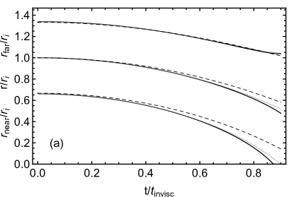
Figure 2: The initial torus shape is $\epsilon_{i}=1/3$ in both cases. Fig. (a) is a low viscosity case ($\mu=0.01\mu_{0}$) and Fig. (b) is a high viscosity case ($\mu=100\mu_{0}$). The continuous lines correspond to our model, the dashed lines to the basic rod model which is equivalent to the viscous string model in this case. The central curves correspond to the central line, the top curves to the outer intersection of the section with the torus plane ($z=0$), and the lower curves to the inner intersection. In Fig. (a), the inviscid solution [Eq. (23)] is depicted in a thin and continuous gray line.

The numerical resolution of the full system of Eqs. (21) and (21) is illustrated in Fig. 2 for typical high and low viscosities. In the low-viscosity case, we also plot the solution to the inviscid equation (23). Given the elliptical deformation of the torus sections, the far and near sides of the section are located respectively at

$$r_{\rm far} = r+R(1-{\cal E}{R}^{2})\,$$ (33)

$$r_{\rm near} = r-R(1-{\cal E}{R}^{2})\,.$$ (34)

We observe that in all cases, the rod model underestimates the shrinking of the central line. The numerical results are in agreement with our expectation that the difference between the two descriptions should be of order of the initial $\epsilon_{R}^{2}=(\kappa{R})^{2}=({R}/r)^{2}$ which we have taken to be $(1/3)^{2}$ in initial conditions. Furthermore, the elliptic deformation reduces even further the distance of the inner intersection of the section with the torus plane ($z=0$) since numerically we get $r_{\rm near}<r-R$. The torus is deformed as if it was squeezed in the azimuthal direction, or as if it was stretched by radial tidal forces. When the inner point reaches a null radius, that is approximately when $r={R}$, the expansion is expected to break down since the ratio $\kappa{R}={R}/r$ reaches unity. Physically it also corresponds to the point where the torus becomes topologically a sphere and an accurate description of the final ringdown toward a sphere must be performed from a multipolar expansion around such a geometry, as e.g. in Ref. Chandrasekhar (1959) for linear dynamics or in Ref. Becker et al. (1994) for non-linear dynamics.

IV Rayleigh-Plateau instability

IV.1 Straight fibers

It is well known that periodic radius perturbations around an infinite straight fiber are unstable for $k{R}<1$, where $k=2\pi/\lambda$ is the mode of the perturbation. This is the celebrated Rayleigh-Plateau (RP) instability Rayleigh (1878); Plateau (1873); Rayleigh (1892); Weber (1931) (see also Refs. Eggers (1997); Eggers and Villermaux (2008) for reviews). In the case of an elongated but finite fiber, the RP has been studied numerically in Ref. Driessen et al. (2013). The RP instability is understood analytically by considering periodic radius perturbations around an infinite cylinder of viscous fluid with radius ${R}_{0}$ of the form

$${R}={R}_{0}+\delta{R}\,,\qquad\delta{R}=\underline{\delta{R}}{\rm e}^{\alpha t}\cos(ks),$$ (35)

and then linearizing the Navier-Stokes equation and the boundary constraint. Using units for which ${R}_{0}=1$ and ${\nu}=1$ for convenience, this leads to the implicit dispersion relation Weber (1931); García and Castellanos (1994)

$$\alpha^{2}\frac{kI_{0}(k)}{2I_{1}(k)}=\tfrac{1}{2}(k^{2}-k^{4})$$ (36)

$$-{\mu}\alpha k^{2}\left[\frac{2kI_{0}(k)}{I_{1}(k)}-1+\frac{2{\mu}k^{2}}{\alpha}\left(\frac{kI_{0}(k)}{I_{1}(k)}-\frac{k_{1}I_{0}(k_{1})}{I_{1}(k_{1})}\right)\right]$$

where the $I_{n}$ are the Bessel’s functions and with

$$k_{1}^{2}\equiv k^{2}+\frac{\alpha}{{\mu}}\,.$$ (37)

It is then found that in the inviscid case, the mode which grows the most rapidly corresponds to $k_{\rm max}R_{0}\simeq 0.69702$, that is

$$\lambda_{\rm max}=\frac{2\pi}{k_{\rm max}}\simeq 9.0144R_{0}\,.$$ (38)

Since Eq. (36) is implicit, it is convenient to expand it in powers of $k$ (still in units where $R_{0}={\nu}=1$), and we get [see Eq. (96) of Ref. García and Castellanos (1994)]

$$\alpha \simeq \frac{k}{\sqrt{2}}-\frac{3{\mu}}{2}k^{2}+\frac{36{\mu}^{2}-9}{16\sqrt{2}}k^{3}+\frac{3{\mu}}{16}k^{4}$$

$$+ \frac{-49+360{\mu}^{2}-1296{\mu}^{4}}{512\sqrt{2}}k^{5}+\left(\frac{1}{3072{\mu}}-\frac{{\mu}}{96}\right)k^{6}\,.$$

Note that this series is not valid in the limit ${\mu}\to 0$. However, it allows to compare the exact result (36) with the one obtained from the straight fiber results found with our method in § VI of Ref. Pitrou (2018). Eqs. (6.10a) for $\partial_{t}v$ [with its ${\cal O}(\epsilon_{R}^{2})$ and ${\cal O}(\epsilon_{R}^{4})$ corrections given in Eqs. (6.23a) and (E1)], together with Eq. (6.3) for $\partial_{t}{R}$ [with its ${\cal O}(\epsilon_{R}^{2})$ and ${\cal O}(\epsilon_{R}^{4})$ corrections given in Eqs. (6.23c) and (E2)], once linearized lead to (still in units where ${\nu}=R_{0}=1$)

$$\partial_{t}v&=-\partial_{s}\delta{\cal K}+3{\mu}\partial_{s}^{2}v+\tfrac{3}{8}{\mu}\partial_{s}^{4}v+\tfrac{1}{48}{\mu}\partial_{s}^{6}v\\ -\tfrac{1}{48{\mu}}\partial_{t}\partial^{3}_{s}\delta{\cal K}+\tfrac{3}{64}\partial_{s}^{5}\delta{\cal K}\,,\\ \partial_{t}\delta R=-\tfrac{1}{2}\partial_{s}v-\tfrac{1}{16}\partial^{3}_{s}v+\tfrac{1}{128}\partial^{5}_{s}v\\ -\tfrac{1}{96{\mu}}\partial_{s}^{4}\delta{\cal K}\,,\\ \delta{\cal K}=-\delta R-\partial_{s}^{2}\delta R\,.$$ (40)

From these we can also determine a dispersion relation. It is achieved by expanding $\delta{R}$ and $\partial_{s}v$ as in Eq. (35). Developing the dispersion relation obtained in powers of $k$, we get

$$\alpha \simeq \frac{k}{\sqrt{2}}-\frac{3{\mu}}{2}k^{2}+\frac{36{\mu}^{2}-9}{16\sqrt{2}}k^{3}+\frac{3{\mu}}{16}k^{4}$$

$$+ \frac{-49+360{\mu}^{2}-1296{\mu}^{4}}{512\sqrt{2}}k^{5}+\left(\frac{1}{1536{\mu}}-\frac{{\mu}}{96}\right)k^{6}\,.$$

One notices that it differs from Eq. (IV.1) only in the terms which are $\propto 1/{\mu}$. This is because our formalism is based on the fact that the fluid has non-vanishing viscosity and is ill defined in the inviscid case. However, we note that cancellations occur for the lowest order and the ${\cal O}(\epsilon_{R}^{2})$ corrections, and these divergent terms occur only when including ${\cal O}(\epsilon_{R}^{4})$ corrections, which contribute only to the $k^{5}$ and $k^{6}$ terms of the expansion and beyond.

IV.2 Instability around torus

We now study how this instability is modified when considering small linear fluctuations around the shrinking torus described previously in § III. In the case where the torus is surrounded by a more viscous fluid than the one in the torus, this was already studied experimentally in Ref. Pairam and Fernández-Nieves (2009) by forming a torus thanks to extrusion through a needle, or in Ref. McGraw et al. (2010) using a glassy transition from solid phase to viscous phase in a polystyrene torus. In both cases, it is found when $R_{i}\ll r_{i}$ that the final state is a breakup of the initial torus into several droplets. This is confirmed by the numerical study of Ref. Mehrabian and J. Feng (2013), which considers quadrupolar perturbations. However, in our case, the torus is not surrounded by a highly viscous fluid which retards its shrinking, hence the dynamics of the RP instability is bound to be different. Our system is in fact very similar to the experiment described in Ref. Darbois Texier et al. (2013) where liquid oxygen is sculpted into a torus thanks to its paramagnetic property, and it differs essentially only in that we have not included gravity. As it levitates one its own vapor, this torus is not subject to external viscous forces. It is found experimentally in Ref. Darbois Texier et al. (2013) that the RP instability is never strong enough to breakup the torus in multiple droplets before its shrinking reduces it topologically to a sphere, a result that we confirm with our model in this section.

Figure 3: The initial aspect ratio is $\epsilon_{i}=0.1$. Fig. (a) : The dots are the adimensionalized growth rate $\alpha R_{i}^{3/2}{\nu}^{-1/2}$ as a function of the mode integer $n$, for an initial shape characterized by $\epsilon_{i}=0.1$. The continuous line corresponds to the result obtained for the Rayleigh-Plateau instability on an infinite straight line. From top to bottom we show the cases $\mu=0.1{\sqrt{{\nu}R_{i}}}$, $\mu={\sqrt{{\nu}R_{i}}}$, and $\mu=10{\sqrt{{\nu}R_{i}}}$.
Fig. (b) : Growth rate relative difference with respect to the one obtained for the Rayleigh-Plateau instability of an infinite straight line. Our model (circles) and the improved rod model (crosses) is evaluated for large symbols with $\mu=0.1\sqrt{{\nu}R_{i}}$ (low viscosity) and for small symbols with $\mu=10^{3}\sqrt{{\nu}R_{i}}$ (high viscosity). In all cases, the dipolar mode ($n=1$) growth rate is identically vanishing as required by center of mass conservation.

When restricting to linear fluctuations around the shrinking torus (that we consider as a background), great simplifications arise because the background quantities, that we note in this section, ${R}_{0}$, $\kappa_{0}$, $r_{0}$, ${\cal E}_{0}$ and $U^{r}_{0}$, do not depend on $\theta$. Hence, we can ignore small angular displacements of the fiber sections due to the fluctuations. In practice, everything happens as if a section which is initially at a given $\theta=s/r$ remains at the same angular position even though $s$ and $r$ vary because of shrinking, indicating that the variables $(t,\theta)$ are more adapted for the problem than $(t,s)$. Note that small angular displacements would only be relevant if we were to consider the non-linear dynamics.

We split variables into their background and their perturbed quantity as

$$\kappa = \kappa_{0}+\delta\kappa\,,$$ (42)

$$r = r_{0}+\delta r\,,$$ (43)

$${\cal E} = {\cal E}_{0}+\delta{\cal E}\,,$$ (44)

$$U^{r} = U^{r}_{0}+\delta U^{r}\,,$$ (45)

$${R} = {R}_{0}+\delta{R}\,,$$ (46)

$$\overline{\cal V} = \overline{\cal V}_{0}+\delta\overline{\cal V}\,.$$ (47)

The dynamics of the background has already been discussed in § III and, considering no torus rotation ($\overline{\cal V}_{0}=0$), it is governed by the differential system (21) in the variables $(r_{0},{\cal E}_{0})$.

For small linear perturbations, we can use the relations

$$\delta\kappa \simeq -\frac{\delta r}{r^{2}}-\partial^{2}_{s}\delta r\,,$$ (48)

$$\delta U^{r} \simeq \partial_{t}\delta r|_{\theta}=\partial_{t}\delta r|_{s}-\bar{U}_{0}\partial_{s}\delta r\,,$$ (49)

so that eventually the perturbed set of variables is

$$(\delta r,\delta{R},\delta\overline{\cal V},\delta{\cal E}).$$ (50)

The linearized equations of our model are reported in the Appendix and one needs only to replace the relations (48) to get a closed system of differential equations in these variables.

We first study the growing modes of the Rayleigh-Plateau instability by considering these equations at initial time, that is, ignoring the effects of the secular background shrinking. When considering periodic perturbation, the variables (50) are expanded as

$$x=\underline{x}{\rm e}^{\alpha t}\cos(n\theta)=\underline{x}{\rm e}^{\alpha t}\cos\left[\frac{ns}{r(t)}\right]\,.$$ (51)

Solving for $\alpha$, we obtain the dispersion relation as a function of the mode $n$. The algebraic expressions for $\alpha$ are far too complex to be reported explicitly. Their numerical values are, however, depicted in the left plot of Fig. 3 where we superimposed the Rayleigh-Plateau dispersion relation (36) obtained in the straight fiber case. The relative differences for our model and for the improved rod model [see Eq. (7.74) of Ref. Pitrou (2018)] are presented in the right plot of Fig. 3, and these differences come from the fact that the models differ in their ${\cal O}(\epsilon_{R}^{2})$ corrections.

We then consider the full system of differential equations in the Appendix and solve for it numerically for different viscosities. We assume that initially the perturbation is only a perturbation in the section radius $\delta R_{i}$, with all other perturbations vanishing. The growth of the linear perturbations is then characterized by $\underline{\delta R}/\underline{\delta R_{i}}$, which characterizes the RP instability, and which is plotted in Figs. 4(a) and 4(b). Additionally, departure from the toroidal geometry of the central line is characterized by the evolution of $\delta r$. Since we consider linear perturbations, its evolution is commensurate with $\delta R_{i}$, hence we plot in Figs. 4(c) and 4(d) $\underline{\delta r}/\underline{\delta R_{i}}$ that indicates how efficiently a deformation of the sections results in a deformation of the central line. The integration for a given mode $n$ is stopped at $t_{\rm end}$ defined by the condition $kR=nR/r=1$, since it corresponds to $\epsilon_{R}=1$, that is, to a breaking of the perturbative expansion in the fiber radius, which is central to the construction of our model. This happens unavoidably because $r$ decreases as the torus shrinks, but also $R$ increases from volume conservation.

• For low viscosities, slightly before $t_{\rm end}$, we see an inflexion point in the perturbation growth. In the light of the RP instability for straight fibers, and considering that modifications brought by the toroidal shape are small, this corresponds to the fact that when $k=n/r>k_{\rm max}$, the value of $\alpha$ in the dispersion relation decreases to reach $\alpha=0$ when $kR=1$. For each mode, everything happens as if the mode was climbing the dispersion relation curve $\alpha(k)$ of the usual straight fiber RP instability from low values of $k$, to high values of $k$, hence passing through the maximum value $\alpha(k_{\rm max})$. And in that process, long modes which correspond to low values of $n$ (but not the dipolar perturbation corresponding to $n=1$ which is otherwise constrained by center of mass conservation) have had more time to grow so as to reach the highest growth. However, we notice that even for the long modes, the typical growth never reaches huge values. This is because the time scale of the RP instability is $t_{\rm RP}\equiv\sqrt{R_{i}^{3}/{\nu}}$ and it is related to the collapse time scale (28) by $t_{\rm RP}=\epsilon_{i}t_{\rm cap}$. The RP instability requires a very thin torus ($\epsilon_{i}\ll 1$) to be able to break it before it has collapsed. Hence, for reasonable values of $\epsilon_{i}$, the RP instability cannot destabilize the toroidal shape and split in several droplets, in agreement with the findings of Ref. Darbois Texier et al. (2013). Hence, for the low viscosity case, the main features of the dynamics can be understood from the perspective of the RP instability around straight fibers. Note that if shrinking is slowed by an external viscous fluid, it is found experimentally Pairam and Fernández-Nieves (2009); McGraw et al. (2010) that these conclusions are reversed.

• For larger viscosities, $k_{\rm max}$ corresponding to the fastest growing mode of RP instability around a straight fiber is much smaller. Indeed, it scales approximately as Driessen et al. (2013) $k_{\rm max}\propto 1/\sqrt{2+3\sqrt{2}\mu}$ (still in units where $R_{0}={\nu}=1$). Furthermore, the corresponding value $\alpha(k_{\rm max})$ is much smaller as illustrated in Fig. 3 (left plot). Hence, if we were to guess the behaviour from the analogous RP instability around straight lines, one would conclude that perturbations do not grow significantly. In fact, we find numerically that perturbations grow indeed mildly, but only up to around $t_{\rm cap}$, as they are damped afterwards. In that case, there is no RP instability and the final state is a single drop.

Figure 4: (a), (b) : $\delta R/\delta R_{i}$. (c), (d) : $\delta r/\delta R_{i}$. The initial shape is characterized by $\epsilon_{i}=0.1$. The viscosity is low ($\mu=0.1\mu_{0}$) for (a) and (c) and high ($\mu=10\mu_{0}$) for (b) and (d). The instability modes are plotted from $n=1$ to $10$ for (a) and (c), or from $n=2$ to $10$ for (b) and (d), starting from the thinnest line to the thickest line.

V Rotating torus

It is possible to prevent the torus from shrinking by considering a torus rotating around the $z$ axis. From angular momentum conservation, this brings a potential barrier and if initial rotation is strong enough, it prevents the collapse of the torus. Indeed, the last term of Eq. (21) acts as a repulsive force. The dynamics of $\overline{\cal V}$, which is not identically vanishing anymore, is ruled by

$$\frac{{\rm d}\overline{\cal V}}{{\rm d}t}=-\overline{\cal V}U^{r}\kappa\left[1-\tfrac{9}{4}(\kappa{R})^{2}\right]\,.$$ (52)

When considering only the leading term in this equation, it can be put in the form ${\rm d}(r\overline{\cal V})/{\rm d}t=0$ which is obviously angular momentum conservation, that is,

$$r\overline{\cal V}=r_{i}\overline{\cal V}_{i}\,.$$ (53)

When the torus shrinks ($U^{r}<0$), $\overline{\cal V}$ must increase. As in the two-body problem of Newtonian gravity, this leads to a repulsive potential $\propto 1/r^{2}$, that is a radial force $\propto 1/r^{3}$ given by the last term of Eq. (21).

Figure 5: For both figures $\overline{\cal V}_{i}=0.8\sqrt{{\nu}/R_{i}}$, $\mu=\mu_{0}$. Fig. (a) : $\epsilon_{i}=1/3$. The continuous lines correspond to our model and the dashed lines correspond to the viscous string model with circular sections. The thick dotted-dashed line is $-{\cal E}{R}^{2}$ whereas the thin dotted-dashed line is $R^{2}/(4r^{2})$. Fig. (b) : $\epsilon_{i}=0.1$ and the lines (from thin to thick) correspond to the modes from $n=1$ to $8$ of $|\delta R|/\delta R_{i}$. The dipolar mode ($n=1$) does not grow because of center of mass conservation.

If rotation is strong enough, the radius $r$ undergoes damped oscillations (except in the pure inviscid case) to reach an equilibrium value. If we ignore the ${\cal O}(\epsilon_{R}^{2})$ corrections, that is, considering only the viscous string model, this is the position for which surface tension attractive force is balanced by the repulsive inertial force, and we find

$$r_{\rm stable}\simeq r_{i}\left(\frac{R_{i}\overline{\cal V}_{i}^{2}}{{\nu}}\right)^{2/5}\,.$$ (54)

Hence, by choosing $\overline{\cal V}_{i}=\sqrt{{\nu}/R_{i}}$ the torus is directly [up to the ${\cal O}(\epsilon_{R}^{2})$ corrections] in its stable position.

Furthermore, now the last term of Eq. (21) contributes and it corresponds to the deformation induced by tidal forces. In the inviscid limit, the constraint (22) becomes

$${\cal E}{R}^{2}\simeq-\frac{(\kappa{R})^{2}}{6}\left(1+\frac{\overline{\cal V}^{2}{R}}{2{\nu}}\right)\,.$$ (55)

Once the radius has reached its equilibrium value (54), the elliptic deformation tends to ${\cal E}{R}^{2}\simeq-R^{2}/(4r^{2})$ as illustrated in the left plot of Fig. 5. We then repeat the linear perturbation analysis of § IV.2, but including all the terms involving $\overline{\cal V}_{0}$ (which we do not report in the Appendix), whose dynamics is given by Eq. (52). Instead of expanding the linear perturbations with $\cos(ns/r)$ as in Eq. (51), we expand them with $\exp({\rm i}ns/r)$. Indeed, the amplitude $\underline{x}$ becomes complex when including torus rotation. Its norm still characterizes the instability, that is the size of the perturbation, and its phase corresponds to the angular rotation induced by advection. In the right plot of Fig. 5, we illustrate how the RP instability can develop freely once the torus has reached a stable rotating solution. Hence it is expected that the initially rotating viscous torus will break up in several droplets that will be ejected outward.

VI Conclusion

The viscous torus allows to clearly emphasize the difference between our model and the viscous string or its refined rod model, since for the main shrinking behaviour these have no corrections of order ${\cal O}(\epsilon_{R}^{2})$ whereas our model does. Our corrections affect the central line dynamics, and we find it necessary to also describe the elliptic deformations. When studying the Rayleigh-Plateau instability, our model and the (improved) rod model also differ slightly as shown by considering the dispersion relation. When the torus is not surrounded by a viscous fluid, our linear analysis indicates that the torus does not break up into small droplets for all possible viscosities, since either the instability does not develop in very viscous fluids or does not have sufficient time to develop in low-viscosity fluids. However, if the torus is rotating around its geometric center fast enough, it can reach an equilibrium configuration around which the RP instability should lead to its unavoidable breakup in several droplets.

Appendix A Linearized viscous torus perturbations

Dynamical equations for the variables (50) are obtained from Eqs. (7.18a), (7.18b), (7.20), and (7.42) and their ${\cal O}(\epsilon_{R}^{2})$ corrections [Eqs. (7.41), (G3), and (G4)] of Ref. Pitrou (2018). After linearizing them, one uses the linearized constraints (7) and (7) to get

$$\partial_{t}\delta\overline{\cal V} = -v_{0}\partial_{s}\delta\overline{\cal V}+U^{r}_{0}\partial_{s}\delta U^{r}-U^{r}_{0}\kappa_{0}\delta\overline{\cal V}+3{\mu}\partial_{s}^{2}\delta\overline{\cal V}+3{\mu}\kappa_{0}\partial_{s}\delta U^{r}+3{\mu}U^{r}_{0}\partial_{s}\delta\kappa+6{\mu}U^{r}_{0}\kappa_{0}\frac{\partial_{s}\delta R}{R_{0}}+\frac{{\nu}\partial_{s}\delta R}{R_{0}^{2}}$$

$$+{\nu}R_{0}\left(\tfrac{3}{4}\kappa_{0}^{2}\frac{\partial_{s}\delta R}{R_{0}}+\tfrac{1}{4}\kappa_{0}\partial_{s}\delta\kappa+\frac{\partial_{s}^{3}\delta R}{R_{0}}+\frac{\partial_{s}^{3}\delta R}{R_{0}}\right)$$

$$+R_{0}^{2}\Big{(}\tfrac{9}{4}U^{r}_{0}\kappa_{0}^{3}\delta\overline{\cal V}+\tfrac{3}{4}(U^{r}_{0})^{2}\kappa_{0}^{2}\frac{\partial_{s}\delta R}{R_{0}}-\tfrac{9}{2}{\mu}U^{r}_{0}\kappa_{0}^{3}\frac{\partial_{s}\delta R}{R_{0}}-\tfrac{15}{8}U^{r}_{0}\kappa_{0}^{2}\partial_{s}\delta U^{r}-\tfrac{63}{16}{\mu}\kappa_{0}^{3}\partial_{s}\delta U^{r}+\tfrac{3}{8}(U^{r}_{0})^{2}\kappa_{0}\partial_{s}\delta\kappa$$

$$\qquad-\tfrac{75}{16}{\mu}U^{r}_{0}\kappa_{0}^{2}\partial_{s}\delta\kappa+\tfrac{3}{8}U^{r}_{0}\kappa_{0}\partial_{s}^{2}\delta\overline{\cal V}-\tfrac{57}{16}{\mu}\kappa_{0}^{2}\partial_{s}^{2}\delta\overline{\cal V}+3{\mu}U^{r}_{0}\kappa_{0}\frac{\partial_{s}^{3}\delta R}{R_{0}}+\tfrac{3}{8}{\mu}U^{r}_{0}\partial_{s}^{3}\delta\kappa+\tfrac{3}{8}{\mu}\partial_{s}^{4}\delta\overline{\cal V}\Big{)}$$

$$\partial_{t}\delta U^{r} = -v_{0}\partial_{s}\delta U^{r}-{\nu}\frac{\delta\kappa}{R_{0}}+{\nu}\kappa_{0}\frac{\delta R}{R_{0}^{2}}-6{\mu}U^{r}_{0}\kappa_{0}\delta\kappa-3{\mu}\kappa_{0}^{2}\delta U^{r}-3{\mu}\kappa_{0}\partial_{s}\delta\overline{\cal V}$$ (57)

$$+{\nu}R_{0}\left(-\tfrac{21}{8}\kappa_{0}^{2}\delta\kappa-\tfrac{7}{8}\kappa_{0}^{3}\frac{\delta R}{R_{0}}-\tfrac{13}{8}\kappa_{0}\frac{\partial_{s}^{2}\delta R}{R_{0}}-\tfrac{3}{4}\partial_{s}^{2}\delta\kappa\right)$$

$$+R_{0}^{2}\Big{(}-\tfrac{63}{16}(U^{r}_{0})^{2}\kappa_{0}^{2}\delta\kappa-\tfrac{21}{8}(U^{r}_{0})^{2}\kappa_{0}^{3}\frac{\delta R}{R_{0}}-\tfrac{21}{8}U^{r}_{0}\kappa_{0}^{3}\delta U^{r}-\tfrac{33}{4}{\mu}U^{r}_{0}\kappa_{0}^{3}\delta\kappa-\tfrac{33}{8}{\mu}U^{r}_{0}\kappa_{0}^{4}\frac{\delta R}{R_{0}}-\tfrac{33}{16}{\mu}\delta U^{r}\kappa_{0}^{4}$$

$$\qquad-\tfrac{3}{8}U^{r}_{0}\kappa_{0}^{2}\partial_{s}\delta\overline{\cal V}-\tfrac{27}{16}{\mu}\kappa_{0}^{3}\partial_{s}\delta\overline{\cal V}-\tfrac{39}{4}{\mu}U^{r}_{0}\kappa_{0}^{2}\frac{\partial_{s}^{2}\delta R}{R_{0}}-\tfrac{9}{4}U^{r}_{0}\kappa_{0}\partial_{s}^{2}\delta U^{r}-\tfrac{9}{2}{\mu}\kappa_{0}^{2}\partial_{s}^{2}\delta U^{r}$$

$$\qquad-\tfrac{27}{4}{\mu}U^{r}_{0}\kappa_{0}\partial_{s}^{2}\delta\kappa-\tfrac{27}{8}{\mu}\kappa_{0}\partial_{s}^{3}\delta\overline{\cal V}-\tfrac{3}{4}{\mu}\partial_{s}^{4}\delta U^{r}\Big{)}$$

$$\partial_{t}\delta{\cal E} = -v_{0}\partial_{s}\delta{\cal E}+{\cal E}_{0}\partial_{s}\delta\overline{\cal V}+\frac{{\nu}}{{\mu}{R}_{0}}\left(\delta{\cal E}+\frac{{\cal E}_{0}\delta R}{R_{0}}-\tfrac{1}{3}\kappa_{0}\delta\kappa+\tfrac{1}{6}\frac{\kappa_{0}^{2}\delta R}{{R}_{0}}\right)+{\cal E}_{0}U^{r}_{0}\delta\kappa+U^{r}_{0}\kappa_{0}\delta{\cal E}+\kappa_{0}{\cal E}_{0}\delta U^{r}$$ (58)

$$-\tfrac{21}{16}U^{r}_{0}\kappa_{0}^{2}\delta\kappa-\tfrac{7}{16}\kappa_{0}^{3}\delta U^{r}-\tfrac{5}{16}\kappa_{0}^{2}\partial_{s}\delta\overline{\cal V}-\tfrac{1}{8}\kappa_{0}\partial_{s}^{2}\delta U^{r}$$

$$\frac{\partial_{t}\delta R}{R_{0}} = -v_{0}\frac{\partial_{s}\delta R}{R_{0}}-\tfrac{1}{2}U^{r}_{0}\delta\kappa-\tfrac{1}{2}\kappa_{0}\delta U^{r}-\tfrac{1}{2}\partial_{s}\delta\overline{\cal V}+R_{0}^{2}\left(-\tfrac{3}{8}U^{r}_{0}\kappa_{0}\frac{\partial_{s}^{2}\delta R}{R_{0}}-\tfrac{1}{16}\kappa_{0}\partial_{s}^{2}\delta U^{r}-\tfrac{1}{16}U^{r}_{0}\partial_{s}^{2}\delta\kappa-\tfrac{1}{16}\partial_{s}^{3}\delta\overline{\cal V}\right)$$ (59)