Riemannian Walk for Incremental Learning: Understanding Forgetting and Intransigence

Abstract

Incremental learning (il) has received a lot of attention recently, however, the literature lacks a precise problem definition, proper evaluation settings, and metrics tailored specifically for the il problem. One of the main objectives of this work is to fill these gaps so as to provide a common ground for better understanding of il. The main challenge for an il algorithm is to update the classifier whilst preserving existing knowledge. We observe that, in addition to forgetting, a known issue while preserving knowledge, il also suffers from a problem we call intransigence, inability of a model to update its knowledge. We introduce two metrics to quantify forgetting and intransigence that allow us to understand, analyse, and gain better insights into the behaviour of il algorithms. We present RWalk, a generalization of ewc++ (our efficient version of ewc [7]) and Path Integral [26] with a theoretically grounded KL-divergence based perspective. We provide a thorough analysis of various il algorithms on MNIST and CIFAR-100 datasets. In these experiments, RWalk obtains superior results in terms of accuracy, and also provides a better trade-off between forgetting and intransigence.

1 Introduction

Realizing human-level intelligence requires developing systems capable of learning new tasks continually while preserving knowledge about the old ones. This is precisely the objective underlying incremental learning (il) algorithms. By definition, il has ever-expanding output space, and limited or no access to data from the previous tasks while learning a new one. This makes il more challenging and fundamentally different from the classical learning paradigm where the output space is fixed and the entire dataset is available. Recently, there have been several works in il [7, 15, 20, 26] with varying evaluation settings and metrics making it difficult to establish fair comparisons. The first objective of this work is to rectify these issues by providing precise definitions, evaluation settings, and metrics for il for the classification task.

Let us now discuss the key points to consider while designing il algorithms. The first question is ‘how to define knowledge: factors that quantify what the model has learned’. Usually, knowledge is defined either using the input-output behaviour of the network [5, 20] or the network parameters [7, 26]. Once the knowledge is defined, the objective then is to preserve and update it to counteract two inherent issues with il algorithms: (1) forgetting: catastrophically forgetting knowledge of previous tasks; and (2) intransigence: inability to update the knowledge to learn a new task. Both of these problems require contradicting solutions and pose a trade-off for any il algorithm.

To capture this trade-off, we advocate the use of measures that evaluate an il algorithm based on its performance on the past and the present tasks in the hope that this will reflect in the algorithm’s behaviour on the future unseen tasks. Taking this into account we introduce two metrics to evaluate forgetting and intransigence. These metrics together with the standard multi-class average accuracy allow us to understand, analyse, and gain better insights into the behaviour of various il algorithms.

Further, we present a generalization of two recently proposed incremental learning algorithms, Elastic Weight Consolidation (ewc) [7], and Path Integral (pi) [26]. In particular, first we show that in ewc, while learning a new task, the model’s likelihood distribution is regularized using a well known second-order approximation of the KL-divergence [1, 18], which is equivalent to computing distance in a Riemannian manifold induced by the Fisher Information Matrix [1]. To compute and update the Fisher matrix, we use an efficient (in terms of memory) and online (in terms of computation) approach, leading to a faster and online version of ewc which we call ewc++. Note that, a similar extension to ewc, called online-ewc, is concurrently proposed by Schwarz et al. [22]. Next, we modify the pi [26] where instead of computing the change in the loss per unit distance in the Euclidean space between the parameters as the measure of sensitivity, we use the approximate KL divergence (distance in the Riemannian manifold) between the output distributions as the distance to compute the sensitivity. This gives us the parameter importance score which is accumulated over the optimization trajectory effectively encoding the information about the all the seen tasks so far. Finally, RWalk is obtained by combining ewc++ and the modified pi.

Furthermore, in order to counteract intransigence, we study different sampling strategies that store a small representative subset ($\leq 5\%$) of the dataset from the previous tasks. This not only allows the network to recall information about the previous tasks but also helps in learning to discriminate current and previous tasks. Finally, we present a thorough analysis to better understand the behaviour of il algorithms on MNIST [11] and CIFAR-100 [8] datasets. To summarize, our main contributions are:

1. New evaluation metrics - Forgetting and Intransigence - to better understand the behaviour and performance of an incremental learning algorithm.

2. ewc++: An efficient and online version of ewc.

3. RWalk: A generalization of ewc++ and pi with theoretically grounded KL-divergence based perspective providing new insights.

4. Analysis of different methods in terms of accuracy, forgetting, and intransigence.

2 Problem Set-up and Preliminaries

Here we define the il problem and discuss the practicality of two different evaluation settings: (a) single-head; and (b) multi-head. In addition, we review the probabilistic interpretation of neural networks and the connection of KL-divergence with the distance in the Riemannian manifold, both of which are crucial to our approach.

2.1 Single-head vs Multi-head Evaluations

We consider a stream of tasks, each corresponding to a set of labels. For the $k$-th task, let $\mathcal{D}_{k}=\{(\mathbf{x}^{k}_{i},y^{k}_{i})\}_{i=1}^{n_{k}}$ be the dataset, where $\mathbf{x}^{k}_{i}\in\mathcal{X}$ is the input and $y^{k}_{i}\in\mathbf{y}^{k}$ the ground truth label, and $\mathbf{y}^{k}$ is the set of labels specific to the task. The main distinction between the single-head and the multi-head evaluations is that, at test time, in single-head, the task identifier ($k$) is unknown, whereas in multi-head, it is given. Therefore, for the single-head evaluation, the objective at the $k$-th task is to learn a function $f_{\theta}:\mathcal{X}\rightarrow\mathcal{Y}^{k}$, where $\mathcal{Y}^{k}=\cup_{j=1}^{k}\mathbf{y}^{j}$ corresponds to all the known labels. For multi-head, as the task identifier is known, $\mathcal{Y}^{k}=\mathbf{y}^{k}$. For example, consider MNIST with $5$ tasks: $\{\{0,1\},\cdots,\{8,9\}\}$; trained in an incremental manner. Then, at the $5$-th task, for a given image, the multi-head evaluation is to predict a class out of two labels $\{8,9\}$ for which the $5$-th task was trained. However, the single-head evaluation at $5$-th task is to predict a label out of all the ten classes $\{0,\cdots,9\}$ that the model has seen thus far.

2.1.1 Why single-head evaluation for il?

In the case of single-head, used by [13, 20], the output space consists of all the known labels. This requires the classifier to learn to distinguish labels from different tasks as well. Since, the tasks are supplied in a sequence in il, while learning a new task, the classifier must also be able to learn the inter-task discrimination with no or limited access to the previous tasks’ data. This is a much harder problem compared to multi-head where the output space contains labels of the current task only. Furthermore, single-head is a more practical setting because knowing the subset of labels to look at a priori, which is the case in multi-head, requires extra supervisory signals, in the form of task descriptors, at test time that reduce the problem complexity. For instance, if the task contains only one label, multi-head evaluation would be equivalent to knowing the ground truth label itself.

2.2 Probabilistic Interpretation of Neural Network Output

If the final layer of a neural network is a soft-max layer and the network is trained using cross entropy loss, then the output may be interpreted as a probability distribution over the categorical variables. Thus, at a given $\theta$, the conditional likelihood distribution learned by a neural network is actually a conditional multinoulli distribution defined as $p_{\theta}(\mathbf{y}|\mathbf{x})=\prod_{j=1}^{K}p_{\theta,j}^{[y=j]}$, where $p_{\theta,j}$ is the soft-max probability of the $j$-th class, $K$ are the total number of classes, $\mathbf{y}$ is the one-hot encoding of length $K$, and $[\cdot]$ is Iverson bracket. A prediction can then be obtained from the likelihood distribution $p_{\theta}(\mathbf{y}|\mathbf{x})$. Typically, instead of sampling, a label with the highest soft-max probability is chosen as the network’s prediction. Note that, if $\mathbf{y}$ corresponds to the ground-truth label then the log-likelihood is exactly the same as the negative of the cross-entropy loss, i.e., if the ground-truth corresponds to the $t$-th index of the one-hot representation of $\mathbf{y}$, then $\log p_{\theta}(\mathbf{y}|\mathbf{x})=\log p_{\theta,t}$ (more details can be found in the supplementary material).

2.3 KL-divergence as the Distance in the Riemannian Manifold

Let $D_{KL}(p_{\theta}\|p_{\theta+\Delta\theta})$ be the KL-divergence [9] between the conditional likelihoods of a neural network at $\theta$ and $\theta+\Delta\theta$, respectively. Then, assuming $\Delta\theta\to 0$, the second-order Taylor approximation of the KL-divergence can be written as $D_{KL}(p_{\theta}\|p_{\theta+\Delta\theta})\approx\frac{1}{2}\Delta\theta^{\top}F_{\theta}\Delta\theta=\frac{1}{2}\|\Delta\theta\|^{2}_{F_{\theta}}$ , where $F_{\theta}$, known as the empirical Fisher Information Matrix [1, 18] at $\theta$, is defined as:

$$F_{\theta}=\operatorname{\mathbb{E}}_{(\mathbf{x},\mathbf{y})\sim\mathcal{D}}\left[\left(\frac{\partial\log p_{\theta}(\mathbf{y}|\mathbf{x})}{\partial\theta}\right)\left(\frac{\partial\log p_{\theta}(\mathbf{y}|\mathbf{x})}{\partial\theta}\right)^{\top}\right]\ ,$$ (1)

where $\mathcal{D}$ is the dataset. Note that, as mentioned earlier, the log-likelihood $\log p_{\theta}(\mathbf{y}|\mathbf{x})$ is the same as the negative of the cross-entropy loss function, thus, $F_{\theta}$ can be seen as the expected loss-gradient covariance matrix. By construction (outer product of gradients), $F_{\theta}$ is positive semi-definite (PSD) which makes it highly attractive for second-order optimization techniques [1, 18, 2, 10, 16]. When $\Delta\theta\to 0$, computing KL-divergence $\frac{1}{2}\|\Delta\theta\|^{2}_{F_{\theta}}$ is equivalent to computing the distance in a Riemannian manifold [12] induced by the Fisher information matrix at $\theta$. Since $F_{\theta}\in{}^{P\times P}$ and $P$ is usually in the order of millions for neural networks, it is practically infeasible to store $F_{\theta}$. To handle this, similar to [7], we assume parameters to be independent of each other (diagonal $F_{\theta}$) which results in the following approximation of the KL-divergence:

$$D_{KL}(p_{\theta}\|p_{\theta+\Delta\theta})\approx\frac{1}{2}\sum_{i=1}^{P}F_{\theta_{i}}\,\Delta\theta_{i}^{2}\ ,$$ (2)

where $\theta_{i}$ is the $i$-th entry of $\theta$. Notice, the diagonal entries of $F_{\theta}$ are the expected square of the gradients, where the expectation is over the entire dataset. This makes $F_{\theta}$ computation expensive as it requires a full forward-backward pass over the dataset.

3 Forgetting and Intransigence

Since the objective is to continually learn new tasks while preserving knowledge about the previous ones, an il algorithm should be evaluated based on its performance both on the past and the present tasks in the hope that this will reflect in algorithm’s behaviour on the future unseen tasks. To achieve this, along with average accuracy, there are two crucial components that must be quantified (1) forgetting: how much an algorithm forgets what it learned in the past; and (2) intransigence: inability of an algorithm to learn new tasks. Intuitively, if a model is heavily regularized over previous tasks to preserve knowledge, it will forget less but have high intransigence. If, in contrast, the regularization is too weak, while the intransigence will be small, the model will suffer from catastrophic forgetting. Ideally, we want a model that suffers less from both, thus efficiently utilizing a finite model capacity. In contrast, if one observes high negative correlation between forgetting and intransigence, which is usually the case, then, it suggests that either the model capacity is saturated or the method does not effectively utilize the capacity. Before defining metrics for quantifying forgetting and intransigence, we first define the multi-class average accuracy which will be the basis for defining the other two metrics. Note, some other task specific measure of correctness (e.g., IoU for object segmentation) can also be used while the definitions of forgetting and intransigence remain the same.

3.0.1 Average Accuracy ($A$)

Let $a_{k,j}\in[0,1]$ be the accuracy (fraction of correctly classified images) evaluated on the held-out test set of the $j$-th task $(j\leq k)$ after training the network incrementally from tasks $1$ to $k$. Note that, to compute $a_{k,j}$, the output space consists of either $\mathbf{y}^{j}$ or $\cup_{j=1}^{k}\mathbf{y}^{j}$ depending on whether the evaluation is multi-head or single-head (refer Sec. 2.1). The average accuracy at task $k$ is then defined as $A_{k}=\frac{1}{k}\sum_{j=1}^{k}a_{k,j}$. The higher the $A_{k}$ the better the classifier, but this does not provide any information about forgetting or intransigence profile of the il algorithm which would be crucial to judge its behaviour.

3.0.2 Forgetting Measure ($F$)

We define forgetting for a particular task (or label) as the difference between the maximum knowledge gained about the task throughout the learning process in the past and the knowledge the model currently has about it. This, in turn, gives an estimate of how much the model forgot about the task given its current state. Following this, for a classification problem, we quantify forgetting for the $j$-th task after the model has been incrementally trained up to task $k>j$ as:

$$f_{j}^{k}=\max_{l\in\{1,\cdots,k-1\}}a_{l,j}-a_{k,j}\ ,\quad\forall j<k\ .$$ (3)

Note, $f_{j}^{k}\in[-1,1]$ is defined for $j<k$ as we are interested in quantifying forgetting for previous tasks. Moreover, by normalizing against the number of tasks seen previously, the average forgetting at $k$-th task is written as $F_{k}=\frac{1}{k-1}\sum_{j=1}^{k-1}f_{j}^{k}$. Lower $F_{k}$ implies less forgetting on previous tasks. Here, instead of $\max$ one could use expectation or $a_{j,j}$ in order to quantify the knowledge about a task in the past. However, taking $\max$ allows us to estimate forgetting along the learning process as explained below.

Positive/Negative Backward Transfer ((P/N)BT):

Backward transfer (BT) is defined in [15] as the influence that learning a task $k$ has on the performance of a previous task ${j<k}$. Since our objective is to measure forgetting, negative forgetting ($f_{j}^{k}<0$) implies positive influence on the previous task or positive backward transfer (PBT), the opposite for NBT. Furthermore, in [15], $a_{j,j}$ is used in place of $\max_{l\in\{1,\cdots,k-1\}}a_{l,j}$ (refer Eq. (3)) which makes the measure agnostic to the il process and does not effectively capture forgetting. To understand this, let us consider an example with 4 tasks trained in an incremental manner. We are interested in measuring forgetting of task 1 after training up to task 4. Let the accuracies be $\{a_{1,1},a_{1,2},a_{1,3},a_{1,4}\}=\{0.7,0.8,0.6,0.5\}$. Here, forgetting measured based on Eq. (3) is $f_{1}^{4}=0.3$, whereas [15] would measure it as $0.2$ (irrespective of the variations in $a_{1,2}$ and $a_{1,3}$). Hence, it does not capture the fact that there was a PBT in the learning process. We believe, it is vital that an evaluation metric of an il algorithm considers such behaviour along the learning process.

3.0.3 Intransigence Measure ($I$)

We define intransigence as the inability of a model to learn new tasks. The effect of intransigence is more prominent in the single-head setting especially in the absence of previous data, as the model is expected to learn to differentiate the current task from the previous ones. Experimentally we show that storing just a few representative samples (refer Sec. 4.2) from the previous tasks improves intransigence significantly. Since we wish to quantify the inability to learn, we compare to the standard classification model which has access to all the datasets at all times. We train a reference/target model with dataset $\bigcup_{l=1}^{k}\mathcal{D}_{l}$ and measure its accuracy on the held-out set of the $k$-th task, denoted as $a_{k}^{*}$. We then define the intransigence for the $k$-th task as:

$$I_{k}=a_{k}^{*}-a_{k,k}\ ,$$ (4)

where $a_{k,k}$ denotes the accuracy on the $k$-th task when trained up to task $k$ in an incremental manner. Note, $I_{k}\in[-1,1]$, and lower the $I_{k}$ the better the model. A reasonable reference/target model can be defined depending on the feasibility to obtain it. In situations where it is highly expensive, an approximation can be proposed.

Positive/Negative Forward Transfer ((P/N)FT):

Since intransigence is defined as the gap between the accuracy of an il algorithm and the reference model, negative intransigence ($I_{k}<0$) implies learning incrementally up to task $k$ positively influences model’s knowledge about it, i.e., positive forward transfer (PFT). Similarly, $I_{k}>0$ implies NFT. However, in [15], FT is quantified as the gain in accuracy compared to the random guess (not a measure of intransigence) which is complementary to our approach.

4 Riemannian Walk for Incremental Learning

We first describe ewc++, an efficient version of the well known ewc [7], and then RWalk which is a generalization of ewc++ and pi [26]. Briefly, RWalk has three key components: (1) a KL-divergence-based regularization over the conditional likelihood $p_{\theta}(\mathbf{y}|\mathbf{x})$ (ewc++); (2) a parameter importance score based on the sensitivity of the loss over the movement on the Riemannian manifold (similar to pi); and (3) strategies to obtain a few representative samples from the previous tasks. The first two components mitigate the effects of catastrophic forgetting, whereas the third handles intransigence.

4.1 Avoiding Catastrophic Forgetting

4.1.1 KL-divergence based Regularization (ewc++)

We learn parameters for the current task such that the new conditional likelihood is close (in terms of KL) to the one learned until previous tasks. To achieve this, we regularize over the conditional likelihood distributions $p_{\theta}(\mathbf{y}|\mathbf{x})$ using the approximate KL-divergence, Eq. (2), as the distance measure. This regularization would preserve the inherent properties of the model about previous tasks as the learning progresses. Thus, given parameters $\theta^{k-1}$ trained sequentially from task $1$ to $k-1$, and dataset $\mathcal{D}_{k}$ for the $k$-th task, the objective is:

$$\operatornamewithlimits{argmin}_{\theta}\tilde{L}^{k}(\theta):=L^{k}(\theta)+\lambda\,D_{KL}\left(p_{\theta^{k-1}}(\mathbf{y}|\mathbf{x})\|p_{\theta}(\mathbf{y}|\mathbf{x})\right)\ ,$$ (5)

where, $\lambda$ is a hyperparameter. Substituting Eq. (2), the KL-divergence component can be written as $D_{KL}\left(p_{\theta^{k-1}}\|p_{\theta}\right)\approx\frac{1}{2}\sum_{i=1}^{P}F_{\theta_{i}^{k-1}}(\theta_{i}-\theta_{i}^{k-1})^{2}\$. Note that, for two tasks, the above regularization is exactly the same as that of ewc [7]. Here we presented it from the KL-divergence based perspective. Another way to look at it would be to consider Fisher for each parameter to be its importance score. The intuitive explanation for this is as follows; since Fisher captures the local curvature of the KL-divergence surface of the likelihood distribution (as it is the component of the second-order term of Taylor approximation, refer Sec. 2.3), higher Fisher implies higher curvature, thus suggests to move less in that direction in order to preserve the likelihood.

In the case of multiple tasks, ewc requires storing Fisher for each task independently ($\mathcal{O}(kP)$ parameters), and regularizing over all of them jointly. This is practically infeasible if there are many tasks and the network has millions of parameters. Moreover, to estimate the empirical Fisher, ewc requires an additional pass at the end of training over the dataset of each task (see Eq. (1)). To address these two issues, we propose ewc++ that (1) maintains single diagonal Fisher matrix as the training over tasks progresses, and (2) uses moving average for its efficient update similar to [16]. Given $F_{\theta}^{t-1}$ at $t-1$, Fisher in ewc++ is updated as:

$$F_{\theta}^{t}=\alpha F_{\theta}^{t}+(1-\alpha)F_{\theta}^{t-1}\ ,$$ (6)

where $F_{\theta}^{t}$ is the Fisher matrix obtained using the current batch and $\alpha\in[0,1]$ is a hyperparameter. Note, $t$ represents the training iterations, thus, computing Fisher in this manner contains information about previous tasks, and also eliminates the additional forward-backward pass over the dataset. At the end of each task, we simply store $F_{\theta}^{t}$ as $F_{\theta^{k-1}}$ and use it to regularize the next task, thus storing only two sets of Fisher at any instant during training, irrespective of the number of tasks. Similar to ewc++, an efficient version of ewc, referred as online-ewc, is concurrently developed in [22].

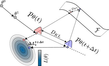
Figure 1: Parameter importance accumulated over the optimization trajectory.

In ewc, Fisher is computed at a local minimum of $\tilde{L}^{k}$ using the gradients of $L^{k}$, which is nearly zero whenever $\tilde{L}^{k}\approx L^{k}$ (e.g., smaller $\lambda$ or when $k=1$). This results in negligible regularization leading to catastrophic forgetting. This issue is partially addressed in ewc++ using moving average. However, to improve it further and to capture model’s behaviour not just at the minimum but also during the entire training process, we augment each element of the diagonal Fisher with a positive scalar as described below. This also ensures that the augmented Fisher is always positive-definite.

4.1.2 Optimization-path based Parameter Importance

Since Fisher captures the intrinsic properties of the model and it only depends on $L^{k}$, it is blinded towards the influence of parameters over the optimization path on the loss surface of $\tilde{L}^{k}$. We augment Fisher with a parameter importance score which is accumulated over the entire training trajectory of $\tilde{L}^{k}$ (similar to [26]). This score is defined as the ratio of the change in the loss function to the distance between the conditional likelihood distributions per step in the parameter space.

More precisely, for a change of parameter from $\theta_{i}(t)$ to $\theta_{i}(t+1)$ (where $t$ is the time step or training iteration), we define parameter importance as the ratio of the change in the loss to its influence in $D_{KL}(p_{\theta(t)}\|p_{\theta(t+1)})$. Intuitively, importance will be higher if a small change in the distribution causes large improvement over the loss. Formally, using the first-order Taylor approximation, the change in loss $L$ can be written as:

$$L(\theta(t+\Delta t))-L(\theta(t))\approx-\sum_{i=1}^{P}\sum_{t=t}^{t+\Delta t}\frac{\partial L}{\partial\theta_{i}}\left(\theta_{i}(t+1)-\theta_{i}(t)\right)=-\sum_{i=1}^{P}\Delta L_{t}^{t+\Delta t}(\theta_{i}),$$ (7)

where $\frac{\partial L}{\partial\theta_{i}}$ is the gradient at $t$, and $\Delta L_{t}^{t+\Delta t}(\theta_{i})$ represents the accumulated change in the loss caused by the change in the parameter $\theta_{i}$ from time step $t$ to $t+\Delta t$. This change in parameter would cause a corresponding change in the model distribution which can be computed using the approximate KL-divergence (Eq. (2)). Thus, the importance of the parameter $\theta_{i}$ from training iteration $t_{1}$ to $t_{2}$ can be computed as $s_{t_{1}}^{t_{2}}(\theta_{i})=\sum_{t=t_{1}}^{t_{2}}\frac{\Delta L_{t}^{t+\Delta t}(\theta_{i})}{\frac{1}{2}F_{\theta_{i}}^{t}\Delta\theta_{i}(t)^{2}+\epsilon}\ ,$ where $\Delta\theta_{i}(t)=\theta_{i}(t+\Delta t)-\theta_{i}(t)$ and $\epsilon>0$. The denominator is computed at every discrete intervals of $\Delta t\geq 1$ and $F_{\theta_{i}}^{t}$ is computed efficiently at every $t$-th step using moving average as described while explaining ewc++. The computation of this importance score is illustrated in Fig. 1. Since we care about the positive influence of the parameters, negative scores are set to zero. Note that, if the Euclidean distance is used instead, the score $s_{t_{1}}^{t_{2}}(\theta_{i})$ would be similar to that of pi [26].

4.1.3 Final Objective Function (RWalk)

We now combine Fisher information matrix based importance and the optimization-path based importance scores as follows:

$$\tilde{L}^{k}(\theta)=L^{k}(\theta)+\lambda\sum_{i=1}^{P}(F_{\theta_{i}^{k-1}}+s_{t_{0}}^{t_{k-1}}(\theta_{i}))(\theta_{i}-\theta_{i}^{k-1})^{2}\ .$$ (8)

Here, $s_{t_{0}}^{t_{k-1}}(\theta_{i})$ is the score accumulated from the first training iteration $t_{0}$ until the last training iteration $t_{k-1}$, corresponding to task $k-1$. Since the scores are accumulated over time, the regularization gets increasingly rigid. To alleviate this and enable continual learning, after each task the scores are averaged: $s_{t_{0}}^{t_{k-1}}(\theta_{i})=\frac{1}{2}\left(s_{t_{0}}^{t_{k-2}}(\theta_{i})+s_{t_{k-2}}^{t_{k-1}}(\theta_{i})\right)$. This continual averaging makes the tasks learned far in the past less influential than the tasks learned recently. Furthermore, while adding, it is important to make sure that the scales of both $F_{\theta_{i}^{k-1}}$ and $s_{t_{0}}^{t_{k-1}}(\theta_{i})$ are in the same order, so that the influence of both the terms is retained. This can be ensured by individually normalizing them to be in the interval $[0,1]$. This, together with score averaging, have a positive side-effect of the regularization hyperparameter $\lambda$ being less sensitive to the number of tasks. Whereas, ewc [7] and pi [26] are highly sensitive to $\lambda$, making them relatively less reliable for il. Note, during training, the space complexity for RWalk is $\mathcal{O}(P)$, independent of the number of tasks.

4.2 Handling Intransigence

Experimentally, we observed that training $k$-th task with $\mathcal{D}_{k}$ leads to a poor test accuracy for the current task compared to previous tasks in the single-head evaluation setting (refer Sec. 2.1). This happens because during training the model has access to $\mathcal{D}_{k}$ which contains labels only for the $k$-th task, $\mathbf{y}^{k}$. However, at test time the label space is over all the tasks seen so far $\mathcal{Y}^{k}=\cup_{j=1}^{k}\mathbf{y}^{j}$, which is much larger than $\mathbf{y}^{k}$. This in turn increases confusion at test time as the predictor function has no means to differentiate the samples of the current task from the ones of previous tasks. An intuitive solution to this problem is to store a small subset of representative samples from the previous tasks and use it while training the current task [20]. Below we discuss different strategies to obtain such a subset. Note that we store $m$ points from each task-specific dataset as the training progresses, however, it is trivial to have a fixed total number of samples for all the tasks similar to iCaRL [20].

4.2.1 Uniform Sampling

A naïve yet highly effective (shown experimentally) approach is to sample uniformly at random from the previous datasets.

4.2.2 Plane Distance-based Sampling

In this case, we assume that samples closer to the decision boundary are more representative than the ones far away. For a given sample $\{\mathbf{x}_{i},y_{i}\}$, we compute the pseudo-distance from the decision boundary $d(\mathbf{x}_{i})=\phi(\mathbf{x}_{i})^{\top}w^{y_{i}}$, where $\phi(\cdot)$ is the feature mapping learned by the neural network and $w^{y_{i}}$ are the last fully connected layer parameters for class $y_{i}$. Then, we sample points based on $q(\mathbf{x}_{i})\propto\frac{1}{d(\mathbf{x}_{i})}$. Here, the intuition is, since the change in parameters is regularized, the feature space and the decision boundaries do not vary much. Hence, the samples that lie close to the boundary would act as boundary defining samples.

4.2.3 Entropy-based Sampling

Given a sample, the entropy of the output soft-max distribution measures the uncertainty of the sample which we used to sample points. The higher the entropy the more likely is that the sample would be picked.

4.2.4 Mean of Features (MoF)

iCaRL [20] proposes a method to find samples based on the feature space $\phi(\cdot)$. For each class $y$, $m$ number of points are found whose mean in the feature space closely approximate the mean of the entire dataset for that class. However, this subset selection strategy is inefficient compared to the above sampling methods. In fact, the time complexity is $\mathcal{O}(nfm)$ where $n$ is dataset size, $f$ is the feature dimension and $m$ is the number of required samples.

5 Related Work

One way to address catastrophic forgetting is by dynamically expanding the network for each new task [25, 19, 21, 24]. Though intuitive and simple, these approaches are not scalable as the size of the network increases with the number of tasks. A better strategy would be to exploit the over-parametrization of neural networks [4]. This entails regularizing either over the activations (output) [20, 14] or over the network parameters [7, 26]. Even though activation-based approach allows more flexibility in parameter updates, it is memory inefficient if the activations are in millions, e.g., semantic segmentation. On the contrary, methods that regularize over the parameters - weighting the parameters based on their individual importance - are suitable for such tasks. Our method falls under the latter category and we show that our method is a generalization of ewc++ and pi [26], where ewc++ is our efficient version of ewc [7], very similar to the concurrently developed online-ewc [22]. Similar in spirit to regularization over the parameters, Lee et al. [13] use moment matching to obtain network weights as the combination of the weights of all the tasks, and Nguyen et al. [17] enforce the distribution over the model parameters to be close via a Bayesian framework. Different from the above approaches, Lopez-Paz et al. [15] update gradients such that the losses of the previous tasks do not increase, while Shin et al. [23] resort to a retraining strategy where the samples of the previous tasks are generated using a learned generative model.

6 Experiments

6.0.1 Datasets

We evaluate baselines and our proposed model - RWalk - on two datasets:

1. Incremental MNIST: The standard MNIST dataset is split into five disjoint subsets (tasks) of two consecutive digits, i.e., $\cup_{k}\mathbf{y}^{k}=\{\{0,1\},\ldots,\{8,9\}\}$.

2. Incremental CIFAR: To show that our approach scales to bigger datasets, we use incremental CIFAR where CIFAR-100 dataset is split into ten disjoint subsets such that $\cup_{k}\mathbf{y}^{k}=\{\{0-9\},\ldots,\{90-99\}\}$.

6.0.2 Architectures

The architectures used are similar to [26]. For MNIST, we use an MLP with two hidden layers each having $256$ units with ReLU nonlinearites. For CIFAR-100, we use a CNN with four convolutional layers followed by a single dense layer (see supplementary for more details). In all experiments, we use Adam optimizer [6] (learning rate = $1\times 10^{-3}$, $\beta_{1}=0.9$, $\beta_{2}=0.999$) with a fixed batch size of $64$.

Table 1: Comparison with different baselines on MNIST and CIFAR in both multi-head and single-head evaluation settings. Baselines where samples are used are appended with ’-S’. For MNIST and CIFAR, 10 (0.2%) and 25(5%) samples are used from the previous tasks using mean of features (MoF) based sampling strategy (refer Sec. 4.2).

c								c	c
c
	$\lambda$	$A_{5}$(%)	$F_{5}$	$I_{5}$	$\lambda$	$A_{10}$(%)	$F_{10}$	$I_{10}$
Vanilla	0	90.3	0.12	$6.6\times 10^{-4}$	0	44.4	0.36	0.02
ewc	75000	99.3	0.001	0.01	$3\times 10^{6}$	72.8	0.001	0.07
pi	0.1	99.3	0.002	0.01	10	73.2	0	0.06
RWalk (Ours)	1000	99.3	0.003	0.01	1000	74.2	0.004	0.04
c
Vanilla	0	38.0	0.62	0.29	0	10.2	0.36	-0.06
ewc	75000	55.8	0.08	0.77	$3\times 10^{6}$	23.1	0.03	0.17
pi	0.1	57.6	0.11	0.8	10	22.8	0.04	0.2
iCaRL-hb1	-	36.6	0.68	-0.01	-	7.4	0.40	0.06
iCaRL	-	55.8	0.19	0.46	-	9.5	0.11	0.35
Vanilla-S	0	73.7	0.30	0.03	0	12.9	0.64	-0.3
ewc-S	75000	79.7	0.14	0.22	$15\times 10^{5}$	33.6	0.27	-0.05
pi-S	0.1	78.7	0.24	0.05	10	33.6	0.27	-0.03
RWalk (Ours)	1000	82.5	0.15	0.14	500	34.0	0.28	-0.06

6.0.3 Baselines

We compare RWalk against the following baselines:

• Vanilla: Network trained without any regularization over past tasks.

• ewc [7] and pi [26]: Both use parameter based regularization. Note, we observed that ewc++ performed at least as good as ewc and therefore, in all the experiments, by ewc we mean the stronger baseline ewc++.

• iCaRL [20]: Uses regularization over the activations and a nearest-exempler-based classifier. Here, iCaRL-hb1 refers to the hybrid1 version, which uses the standard neural network classifier. Both the versions use previous samples.

Note, we use a few samples from the previous tasks to consolidate our baselines further in the single-head setting.

6.1 Results

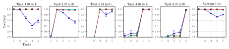
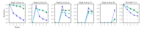
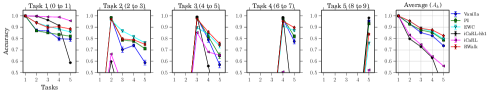
Figure 2: Accuracy on incremental MNIST with multi-head evaluation (top), and single-head evaluation without (middle) and with samples (bottom). First five columns show the variation in performance for different tasks, e.g., the first plot depicts the performance variation on Task 1 when trained incrementally over five tasks. The last column shows the accuracy ($A_{k}$, refer Sec. 3). Mean of features (MoF) sampling is used.

We report the results in Tab. 1 where RWalk outperforms all the baselines in terms of average accuracy and provides better trade-off between forgetting and intransigence. We now discuss the results in detail.

In the multi-head evaluation setting [26, 15], except Vanilla, all the methods provide state-of-the-art accuracy with almost zero forgetting and intransigence (top row of Fig. 2). This gives an impression that il problem is solved. However, as discussed in Sec. 2.1, this is an easier evaluation setting and does not capture the essence of il.

However, in the single-head evaluation, forgetting and intransigence increase substantially due to the the inability of the network to differentiate among tasks. Hence, the performance significantly drops for all the methods (refer Tab. 1 and the middle row of Fig. 2). For instance, on MNIST, forgetting and intransigence of Vanilla deteriorates from $0.12$ to $0.62$, and $6.6\times 10^{-4}$ to $0.29$, respectively, causing the average accuracy to drop from $90.3$% to $38.0$%. Although, regularized methods, ewc and pi, designed to counter catastrophic forgetting, result in less degradation of forgetting, their accuracy is still significantly worse - compare $99.3$% of pi in multi-head against $57.6$% in single-head. In Tab. 1, a similar performance decrease is observed on CIFAR-100 as well. Such a degradation in accuracy even with less forgetting shows that it is not only important to preserve knowledge (quantified by forgetting) but also to update knowledge (captured by intransigence) to achieve better performance. Task-level analysis for CIFAR dataset, similar to Fig. 2, is presented in the supplementary material.

We now show that even with a few representative samples intransigence can be mitigated. For example, in the case of pi on MNIST with only $10$ ($\approx 0.2$%) samples for each previous class, the intransigence drops from $0.8$ to $0.05$ which results in improving the average accuracy from $57.6$% to $78.7$%. Similar improvements can be seen for other methods as well. On CIFAR-100, with only $5$% representative samples, almost identical behaviour is observed.

In our CIFAR-100 experiments (CNN instead of ResNet32), we note that the performance of iCaRL [20] is significantly worse than what has been reported by the authors. We believe this is due to the dependence of iCaRL on a highly expressive feature space, as both the regularization and the classifier depend on it. Perhaps, this reduced expressivity of the feature space due to the smaller network resulted in the performance loss.

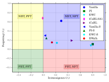
(a) MNIST

(b) CIFAR

Figure 3: Interplay between forgetting and intransigence.

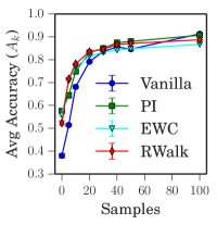
(a) MNIST

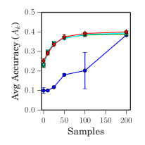
(b) CIFAR

Figure 4: Comparison by increasing the number of samples. On MNIST and CIFAR each class has around 5000 and 500 samples, respectively. With increasing number of samples, the performance of Vanilla improved, but in the range where Vanilla is poor, RWalk consistently performs the best. Uniform sampling is used.

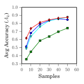
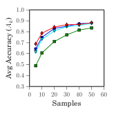
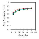
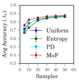
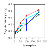
(a) Vanilla

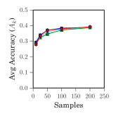
(b) pi

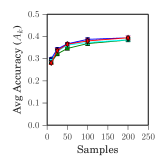
(c) ewc

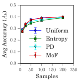
(d) RWalk

Figure 5: Comparison of different sampling strategies discussed in Sec. 4.2 on MNIST (top) and CIFAR-100 (bottom). Mean of features (MoF) outperforms others.

6.1.1 Interplay of Forgetting and Intransigence

In Fig. 3 we study the interplay of forgetting and intransigence in the single-head setting. Ideally we would like a model to be in the quadrant marked as PBT, PFT (i.e., positive backward transfer and positive forward transfer). On MNIST, since all the methods, except iCaRL-hb1, lie on the top-right quadrant, hence for models with comparable accuracy, a model which has the smallest distance from $(0,0)$ would be better. As evident, RWalk is closest to $(0,0)$, providing a better trade-off between forgetting and intransigence compared to all the other methods. On CIFAR-100, the models lie on both the top quadrants and with the introduction of samples, all the regularized methods show positive forward transfer. Since the models lie on different quadrants, their comparison of forgetting and intransigence becomes application specific. In some cases, we might prefer a model that performs well on new tasks (better intransigence), irrespective of its performance on the old ones (can compromise forgetting), and vice versa. Note that, RWalk maintains comparable performance to other baselines while yielding higher average accuracy on CIFAR-100.

6.1.2 Effect of Increasing the Number of Samples

As expected, for smaller number of samples, regularized methods perform far superior compared to Vanilla (refer Fig. 4). However, once the number of samples are sufficiently large, Vanilla starts to perform better or equivalent to the regularized models. The reason is simple because now the Vanilla has access to enough samples of the previous tasks to relearn them at each step, thereby obviating the need of regularized models. However, in an il problem, a fixed small-sized memory budget is usually assumed. Therefore, one cannot afford to store large number of samples from previous tasks. Additionally, for a simpler dataset like MNIST, Vanilla quickly catches up to the regularized models with small number of samples ($20$, $0.4$% of total samples) but on a more challenging dataset like CIFAR it takes considerable amount of samples ($200$, $40$% of total samples) of previous tasks for Vanilla to match the performance of the regularized models.

6.1.3 Comparison of Different Sampling Strategies

In Fig. 5 we compare different subset selection strategies discussed in Sec. 4.2. It can be observed that for all the methods Mean-of-Features (MoF) subset selection procedure, introduced in iCaRL [20], performs the best. Surprisingly, uniform sampling, despite being simple, is as good as more complex MoF, Plane Distance (PD) and entropy-based sampling strategies. Furthermore, the regularized methods remain insensitive to different sampling strategies, whereas in Vanilla, performance varies a lot against different strategies. We believe this is due to the unconstrained change in the last layer weights of the previous tasks.

7 Discussion

In this work, we analyzed the challenges in the incremental learning problem, namely, catastrophic forgetting and intransigence, and introduced metrics to quantify them. Such metrics reflect the interplay between forgetting and intransigence, which we believe will encourage future research for exploiting model capacity, such as, sparsity enforcing regularization, and exploration-based methods for incremental learning. In addition, we have presented an efficient version of ewc referred to as ewc++, and a generalization of ewc++ and pi with a KL-divergence-based perspective. Experimentally, we observed that these parameter regularization methods suffer from high intransigence in the practical single-head setting and showed that this can be alleviated with a small subset of representative samples. Since these methods are memory efficient compared to knowledge distillation-based algorithms such as iCaRL, future research in this direction would enable the possibility of incremental learning on segmentation tasks.

Supplementary Material

For the sake of completeness, we first give more details on the KL-divergence approximation using Fisher information matrix (Sec. 2.3). In particular, we give the proof of KL approximation, $D_{KL}(p_{\theta}\|p_{\theta+\Delta\theta})\approx\frac{1}{2}\Delta\theta^{\top}F_{\theta}\Delta\theta$, discuss the difference between the true Fisher and the empirical Fisher, and explain why the Fisher goes to zero at a minimum. Later, in Sec. 0.B.1, we provide a comparison with GEM [15] and show that RWalk significantly outperforms it. Note that, comparison with GEM is not available in the main paper. Additionally, we discuss the sensitivity of different models to the regularization hyperparameter ($\lambda$) in Sec. 0.B.2. Finally, we conclude in Sec. 0.B.3 with the details of the architecture and task-based analysis of the network used for CIFAR-100 dataset. We note that with additional experiments and further analysis in this supplementary the conclusions of the main paper hold.

Appendix 0.A Approximate KL divergence using Fisher Information Matrix

0.A.1 Proof of Approximate KL divergence

Lemma 1

Assuming $\Delta\theta\to 0$, the second-order Taylor approximation of KL-divergence can be written [1, 18] as:

$$D_{KL}(p_{\theta}\|p_{\theta+\Delta\theta})\approx\frac{1}{2}\Delta\theta^{\top}{F}_{\theta}\Delta\theta\ ,$$ (9)

where $F_{\theta}$ is the empirical Fisher at $\theta$.

Proof

The KL divergence is defined as:

$$D_{KL}(p_{\theta}(\mathbf{z})\|p_{\theta+\Delta\theta}(\mathbf{z}))=\operatorname{\mathbb{E}}_{\mathbf{z}}\left[\log p_{\theta}(\mathbf{z})-\log p_{\theta+\Delta\theta}(\mathbf{z})\right]\ .$$ (10)

Note that we use the shorthands $p_{\theta}(\mathbf{z})=p_{\theta}(\mathbf{y}|\mathbf{x})$ and $\operatorname{\mathbb{E}}_{\mathbf{z}}[\cdot]=\operatorname{\mathbb{E}}_{\mathbf{x}\sim\mathcal{D},\mathbf{y}\sim p_{\theta}(\mathbf{y}|\mathbf{x})}[\cdot]$. We denote partial derivatives as column vectors. Let us first write the second order Taylor series expansion of $\log p_{\theta+\Delta\theta}(\mathbf{z})$ at $\theta$:

$$\log p_{\theta+\Delta\theta}\approx\log p_{\theta}+\Delta\theta^{\top}\frac{\partial\log p_{\theta}}{\partial\theta}+\frac{1}{2}\Delta\theta^{\top}\frac{\partial^{2}\log p_{\theta}}{\partial\theta^{2}}\Delta\theta\ .$$ (11)

Now, by substituting this in Eq. (10), the KL divergence can be approximated as:

$$D_{KL}(p_{\theta}\|p_{\theta+\Delta\theta})\approx\operatorname{\mathbb{E}}_{\mathbf{z}}[\log p_{\theta}]-\operatorname{\mathbb{E}}_{\mathbf{z}}[\log p_{\theta}]$$ (12a)

$$\quad-\Delta\theta^{\top}\operatorname{\mathbb{E}}_{\mathbf{z}}\left[\frac{\partial\log p_{\theta}}{\partial\theta}\right]-\frac{1}{2}\Delta\theta^{\top}\operatorname{\mathbb{E}}_{\mathbf{z}}\left[\frac{\partial^{2}\log p_{\theta}}{\partial\theta^{2}}\right]\Delta\theta\ ,$$

$$=\frac{1}{2}\Delta\theta^{\top}\operatorname{\mathbb{E}}_{\mathbf{z}}\left[-\frac{\partial^{2}\log p_{\theta}}{\partial\theta^{2}}\right]\Delta\theta\quad\mbox{see Eq.~{}\eqref{eq:exp_zero}}\ ,$$

$$=\frac{1}{2}\Delta\theta^{\top}\bar{H}\Delta\theta\quad\mbox{see Eq.~{}\eqref{subeq:hessian_fisher_b}}\ .$$ (12b)

In Eq. (12a), since the expectation is taken such that, $\mathbf{x}\sim\mathcal{D},\mathbf{y}\sim p_{\theta}(\mathbf{y}|\mathbf{x})$, the first order partial derivatives cancel out, i.e.,

$$\operatorname{\mathbb{E}}_{\mathbf{z}}\left[\frac{\partial\log p_{\theta}(\mathbf{z})}{\partial\theta}\right] =\operatorname{\mathbb{E}}_{\mathbf{x}\sim\mathcal{D}}\left[\sum_{\mathbf{\mathbf{y}}}p_{\theta}(\mathbf{\mathbf{y}|\mathbf{x}})\frac{\partial\log p_{\theta}(\mathbf{y}|\mathbf{x})}{\partial\theta}\right]\ ,$$ (13)

$$=\operatorname{\mathbb{E}}_{\mathbf{x}\sim\mathcal{D}}\left[\sum_{\mathbf{\mathbf{y}}}p_{\theta}(\mathbf{y}|\mathbf{x})\frac{1}{p_{\theta}(\mathbf{y}|\mathbf{x})}\frac{\partial p_{\theta}(\mathbf{y}|\mathbf{x})}{\partial\theta}\right]\ ,$$

$$=\operatorname{\mathbb{E}}_{\mathbf{x}\sim\mathcal{D}}\left[\frac{\partial}{\partial\theta}\sum_{\mathbf{\mathbf{y}}}p_{\theta}(\mathbf{y}|\mathbf{x})\right]\ ,$$

$$=\operatorname{\mathbb{E}}_{\mathbf{x}\sim\mathcal{D}}[0]=0\ .$$

Note that this holds for the continuous case as well where, assuming sufficient smoothness and the fact that limits of integration are constants ($0$ to $1$), the Leibniz’s rule would allow us to interchange the differentiation and integration operators.

Additionally, in Eq. (12b), the expected value of negative of the Hessian can be shown to be equal to the true Fisher matrix ($\tilde{F}$) by using Information Matrix Equality.

$$\operatorname{\mathbb{E}}_{\mathbf{z}}\left[-\frac{\partial^{2}\log p_{\theta}(\mathbf{z})}{\partial\theta^{2}}\right]=-\operatorname{\mathbb{E}}_{\mathbf{z}}\left[\frac{1}{p_{\theta}(\mathbf{z})}\frac{\partial^{2}p_{\theta}(\mathbf{z})}{\partial\theta^{2}}\right]\,$$ (14a)

$$\quad+\operatorname{\mathbb{E}}_{\mathbf{z}}\left[\left(\frac{\partial\log p_{\theta}(\mathbf{z})}{\partial\theta}\right)\left(\frac{\partial\log p_{\theta}(\mathbf{z})}{\partial\theta}\right)^{\top}\right]\ ,$$

$$=-\operatorname{\mathbb{E}}_{\mathbf{z}}\left[\frac{1}{p_{\theta}(\mathbf{z})}\frac{\partial^{2}p_{\theta}(\mathbf{z})}{\partial\theta^{2}}\right]+\tilde{F}_{\theta}\ .$$ (14b)

• By the definition of KL-divergence, the expectation in the above equation is taken such that, $\mathbf{x}\sim\mathcal{D},\mathbf{y}\sim p_{\theta}(\mathbf{y}|\mathbf{x})$. This cancels out the first term by following a similar argument as in Eq. (13). Hence, in this case, the expected value of negative of the Hessian equals true Fisher matrix ($\tilde{F}$).

• However, if in Eq. (14b), the expectation is taken such that, $(\mathbf{x},\mathbf{y})\sim\mathcal{D}$, the first term does not go to zero, and $\tilde{F}_{\theta}$ becomes the empirical Fisher matrix ($F_{\theta}$).

• Additionally, at the optimum, since the model distribution approaches the true data distribution, hence even sampling from dataset i.e., $(\mathbf{x},\mathbf{y})\sim\mathcal{D}$ will make the first term to approach zero, and $\bar{H}\approx F_{\theta}$.

With the approximation that $\bar{H}\approx\tilde{F}_{\theta}\approx F_{\theta}$, the proof is complete.

We will argue in Section 0.A.2.2 that the true Fisher matrix is expensive to compute as it requires multiple backward passes. Therefore, as mostly used in literature [1, 18], we also employ empirical Fisher approximation to obtain the KL-divergence.

0.A.2 Empirical vs True Fisher

Loss gradient

Let $q$ be any reference distribution and $p$ (parametrized by $\theta$) be the model distribution obtained after applying softmax on the class scores ($s$). The cross-entropy loss between $q$ and $p$ can be written as: $\ell(\theta)=-\sum_{j}q_{j}\log p_{j}$. The gradients of the loss with respect to the class scores are:

$$\frac{\partial\ell(\theta)}{\partial s_{j}}=p_{j}-q_{j}\ .$$ (15)

By chain rule, the loss gradients w.r.t. the model parameters are $\frac{\partial\ell(\theta)}{\partial\theta}=\frac{\partial\ell(\theta)}{\partial\mathbf{s}}\frac{\partial\mathbf{s}}{\partial\theta}$.

0.A.2.1 Empirical Fisher

In case of an empirical Fisher, the expectation is taken such that $(\mathbf{x},\mathbf{y})\sim\mathcal{D}$. Since every input $\mathbf{x}$ has only one ground truth label, this makes $q$ a Dirac delta distribution . Then, Eq. (15) becomes:

$$\frac{\partial\ell(\theta)}{\partial s_{j}}=\begin{cases}p_{j}-1,&\text{if `$j$' is the ground truth label}\ ,\\ p_{j},&\text{otherwise}\ .\end{cases}$$

Since at any optimum the loss-gradient approaches to zero, thus, Fisher being the expected loss-gradient covariance matrix would also approach to a zero matrix.

0.A.2.2 True Fisher

In case of true Fisher, given $\mathbf{x}$, the expectation is taken such that $\mathbf{y}$ is sampled from the model distributions $p_{\theta}(\mathbf{y}|\mathbf{x})$. If the final layer of a neural network is a soft-max layer and the network is trained using cross entropy loss, then the output may be interpreted as a probability distribution over the categorical variables. Thus, at a given $\theta$, the conditional likelihood distribution learned by a neural network is actually a conditional multinoulli distribution defined as $p_{\theta}(\mathbf{y}|\mathbf{x})=\prod_{j=1}^{K}p_{\theta,j}^{[y=j]}$, where $p_{\theta,j}$ is the soft-max probability of the $j$-th class, $K$ are the total number of classes, $\mathbf{y}$ is the one-hot encoding of length $K$, and $[\cdot]$ is Iverson bracket. At a good optimum, the model distribution $p_{\theta}(\mathbf{y}|\mathbf{x})$ becomes peaky around the ground truth label, implying $p_{\theta,t}\gg p_{\theta,j},\forall j\neq t$ where $t$ is the ground-truth label. Thus, given input $\mathbf{x}$, the model distribution $p_{\theta}(\mathbf{y}|\mathbf{x})$ approach the ground-truth output distribution. This makes the true and empirical Fisher behave in a very similar manner. Note, in order to compute the expectation over the model distribution, the true Fisher requires multiple backward passes making it prohibitively expensive to compute. The standard practice is to resort to the empirical Fisher approximation in this situation [1, 18].

Appendix 0.B Additional Experiments and Analysis

0.B.1 Comparison with GEM [15] on ResNets

Table 2: Following GEM, all the results on ResNets are in the multi-head evaluation setting. Note that, the total number of samples are from all the tasks combined.

Methods	Total Number of Samples	$A_{k}$ (%)
iCaRL	5120	50.8
GEM	5120	65.4
RWalk (Ours)	5000	70.1

In this section we show experiments with ResNet18 [3] on CIFAR-100 dataset. In Tab. 2 we report the results where we compare our method with iCaRL [20] and Gradient Episodic Memory (GEM) [15]. Both of these methods use ResNet18 as an underlying architecture. Following GEM-setup, we split the CIFAR-100 dataset in $20$ tasks where each task consists of $5$ consecutive classes, such that $\cup_{k=1}^{20}\mathbf{y}^{k}=\{\{0-4\},\{5-9\},\ldots,\{95-99\}\}$. Note, following GEM, all the algorithms are evaluated in multi-head setting (refer Sec. 2.1 of the main paper). We refer GEM [15] to report the accuracies of iCaRL and GEM. From the Tab. 2, it can be seen that RWalk outperforms both the methods by a significant margin.

0.B.2 Effect of Regularization Hyperparameter ($\lambda$)

In Tab. 3 we analyse the sensitivity of different methods to the regularization hyperparameter ($\lambda$). As evident, RWalk is less sensitive to $\lambda$ compared to ewc  [7] and PI [26]. This is because of the normalization of the Fisher and Path-based importance scores in RWalk. For example, as we vary $\lambda$ by a factor of $1\times 10^{5}$ on MNIST, the forgetting and intransigence measures changed by $-0.06$ and $0.14$ on ewc [7], and $-0.07$ and $0.13$ on pi [26], respectively. On the other hand, the change in RWalk, as can be seen in the Tab. 3, is $0$ for both the measures. On CIFAR-100 a similar trend is observed in Tab. 3.

Table 3: Comparison of different methods on MNIST and CIFAR-100 as the regularization strength ($\lambda$) is varied. With Forgetting and Intransigence we also provide the change ($\Delta$) in the corresponding measures, where the first row in each method is taken as the reference. As discussed in Sec. 4.1 in the main paper, RWalk is less sensitive to $\lambda$ compared to ewc and pi, making it more appealing for incremental learning.

c									c	c
	$\lambda$	$A_{5}$(%)	$F_{5}(\Delta)$	$I_{5}(\Delta)$	$\lambda$	$A_{10}$(%)	$F_{10}(\Delta)$	$I_{10}(\Delta)$
ewc	75	80.3	0.19 (0)	0.1 (0)	3.0	28.9	0.38 (0)	-0.17 (0)
	$75\times 10^{3}$	79.2	0.15 (-0.04)	0.21 (0.11)	300	34.1	0.28 (-0.1)	-0.07 (0.1)
	$75\times 10^{5}$	79.1	0.13 (-0.06)	0.24 (0.14)	$3\times 10^{5}$	33.7	0.27 (-0.11)	-0.03 (0.14)
pi	0.1	79.3	0.23 (0)	0.05 (0)	0.1	34.7	0.27 (0)	-0.07 (0)
	100	80.3	0.15 (-0.08)	0.22 (0.17)	10	34.3	0.26 (-0.01)	-0.04 (0.03)
	10000	78.5	0.16 (-0.07)	0.18 (0.13)	$1\times 10^{4}$	33.7	0.27 (0)	-0.06 (0.01)
RWalk (Ours)	0.1	82.6	0.16 (0)	0.12 (0)	0.1	34.5	0.28 (0)	-0.06 (0)
	100	81.6	0.16 (0)	0.14 (0.02)	10	33.2	0.28 (0)	-0.06 (0)
	10000	81.6	0.16 (0)	0.12 (0)	$1\times 10^{4}$	34.2	0.28 (0)	-0.05 (0.01)

0.B.3 CIFAR Architecture and Task-Level Analysis

In Tab. 4 we report the detailed architecture of the convolutional network used in the incremental CIFAR-100 experiments (Sec. 6). Note that, in contrast to pi [26], we use only one fully-connected layer (denoted as ‘FC’ in the table). For each task $k$, the weights in the last layer of the network is dynamically added. Additionally, in Fig 6, we present a similar task-level analysis on CIFAR-100 as done for MNIST (Fig. 2 in the main paper). Note that, for all the experiments ‘$\alpha$’ in Eq. (6) is set to $0.9$ and ‘$\Delta t$’ in Eq. (7) is $10$ and $50$ for MNIST and CIFAR, respectively.

Table 4: CNN architecture for incremental CIFAR-100 used for Vanilla, ewc, pi, iCaRl, RWalk in the main paper. Here, ‘$n$’ denotes the number of classes in each task.

Operation	Kernel	Stride	Filters	Dropout	Nonlin.
3x32x32 input
Conv	$3\times 3$	$1\times 1$	$32$		ReLU
Conv	$3\times 3$	$1\times 1$	$32$		ReLU
MaxPool		$2\times 2$		$0.5$
Conv	$3\times 3$	$1\times 1$	$64$		ReLU
Conv	$3\times 3$	$1\times 1$	$64$		ReLU
MaxPool		$2\times 2$		$0.5$
Task 1: FC			$n$
$\cdots$: FC			$n$
Task k: FC			$n$

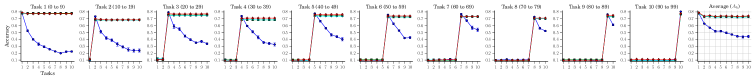
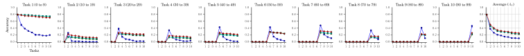
Figure 6: Accuracy measure in incremental CIFAR-100 with multi-head evaluation (top), and the single-head evaluation without (middle) and with samples (bottom). The first ten columns show how the performance of different tasks vary as the model is trained for new tasks, e.g., the first plot depicts the variation in performance on Task 1 when the network is sequentially trained for the ten tasks in an incremental manner. The last column shows the average accuracy measure ($A_{k}$, by varying $k$). Mean of features (MoF) sampling is used. (best viewed in color)

References

- [1] Amari, S.I.: Natural gradient works efficiently in learning. Neural Computation (1998)
- [2] Grosse, R., Martens, J.: A kronecker-factored approximate fisher matrix for convolution layers. In: ICML (2016)
- [3] He, K., Zhang, X., Ren, S., Sun, J.: Deep residual learning for image recognition. In: Proceedings of the IEEE conference on computer vision and pattern recognition. pp. 770–778 (2016)
- [4] Hecht-Nielsen, R., et al.: Theory of the backpropagation neural network. Neural Networks 1(Supplement-1), 445–448 (1988)
- [5] Hinton, G., Vinyals, O., Dean, J.: Distilling the knowledge in a neural network. In: NIPS (2014)
- [6] Kingma, D., Ba, J.: Adam: A method for stochastic optimization. In: ICLR (2015)
- [7] Kirkpatrick, J., Pascanu, R., Rabinowitz, N.C., Veness, J., Desjardins, G., Rusu, A.A., Milan, K., Quan, J., Ramalho, T., Grabska-Barwinska, A., Hassabis, D., Clopath, C., Kumaran, D., Hadsell, R.: Overcoming catastrophic forgetting in neural networks. Proceedings of the National Academy of Sciences of the United States of America (PNAS) (2016)
- [8] Krizhevsky, A., Hinton, G.: Learning multiple layers of features from tiny images. https://www.cs.toronto.edu/ kriz/cifar.html (2009)
- [9] Kullback, S., Leibler, R.A.: On information and sufficiency. The Annals of Mathematical Statistics (1951)
- [10] Le Roux, N., Pierre-Antoine, M., Bengio, Y.: Topmoumoute online natural gradient algorithm. In: NIPS (2007)
- [11] LeCun, Y.: The mnist database of handwritten digits. http://yann. lecun. com/exdb/mnist/ (1998)
- [12] Lee, J.M.: Riemannian manifolds: an introduction to curvature, vol. 176. Springer Science & Business Media (2006)
- [13] Lee, S.W., Kim, J.H., Ha, J.W., Zhang, B.T.: Overcoming catastrophic forgetting by incremental moment matching. In: NIPS (2017)
- [14] Li, Z., Hoiem, D.: Learning without forgetting. In: ECCV (2016)
- [15] Lopez-Paz, D., Ranzato, M.: Gradient episodic memory for continuum learning. In: NIPS (2017)
- [16] Martens, J., Grosse, R.: Optimizing neural networks with kronecker-factored approximate curvature. In: ICML (2015)
- [17] Nguyen, C.V., Li, Y., Bui, T.D., Turner, R.E.: Variational continual learning. ICLR (2018)
- [18] Pascanu, R., Bengio, Y.: Revisiting natural gradient for deep networks. In: ICLR (2014)
- [19] Rebuffi, S.A., Bilen, H., Vedaldi, A.: Learning multiple visual domains with residual adapters. In: NIPS (2017)
- [20] Rebuffi, S.V., Kolesnikov, A., Lampert, C.H.: iCaRL: Incremental classifier and representation learning. In: CVPR (2017)
- [21] Rusu, A.A., Rabinowitz, N.C., Desjardins, G., Soyer, H., Kirkpatrick, J., Kavukcuoglu, K., Pascanu, R., Hadsell, R.: Progressive neural networks. arXiv preprint arXiv:1606.04671 (2016)
- [22] Schwarz, J., Luketina, J., Czarnecki, W.M., Grabska-Barwinska, A., Teh, Y.W., Pascanu, R., Hadsell, R.: Progress & compress: A scalable framework for continual learning. In: ICML (2018)
- [23] Shin, H., Lee, J.K., Kim, J., Kim, J.: Continual learning with deep generative replay. In: NIPS (2017)
- [24] Terekhov, A.V., Montone, G., O’Regan, J.K.: Knowledge transfer in deep block-modular neural networks. In: Conference on Biomimetic and Biohybrid Systems. pp. 268–279 (2015)
- [25] Yoon, J., Yang, E., Lee, J., Hwang, S.J.: Lifelong learning with dynamically expandable networks. In: ICLR (2018)
- [26] Zenke, F., Poole, B., Ganguli, S.: Continual learning through synaptic intelligence. In: ICML (2017)