An Iterative Spanning Forest Framework for Superpixel Segmentation

Abstract

Superpixel segmentation has become an important research problem in image processing. In this paper, we propose an Iterative Spanning Forest (ISF) framework, based on sequences of Image Foresting Transforms, where one can choose i) a seed sampling strategy, ii) a connectivity function, iii) an adjacency relation, and iv) a seed pixel recomputation procedure to generate improved sets of connected superpixels (supervoxels in 3D) per iteration. The superpixels in ISF structurally correspond to spanning trees rooted at those seeds. We present five ISF methods to illustrate different choices of its components. These methods are compared with approaches from the state-of-the-art in effectiveness and efficiency. The experiments involve 2D and 3D datasets with distinct characteristics, and a high level application, named sky image segmentation. The theoretical properties of ISF are demonstrated in the supplementary material and the results show that some of its methods are competitive with or superior to the best baselines in effectiveness and efficiency.

I Introduction

Superpixels has emerged as an important topic in image processing. They group pixels into perceptually meaningful atomic regions [1]. A superpixel can be conceived as a region of similar and connected pixels. Since all the pixels in the same superpixel exhibit similar characteristics, superpixel primitives are computationally much more efficient than their pixel counterparts. It is also expected that the image objects be defined by the union of their superpixels. Satisfied this property, superpixels can be used for a variety of applications: medical image segmentation [2], sky segmentation [3], motion segmentation [4], multi-class object segmentation [5], [6], object detection [7], spatiotemporal saliency detection [8], target tracking [9], and depth estimation [10].

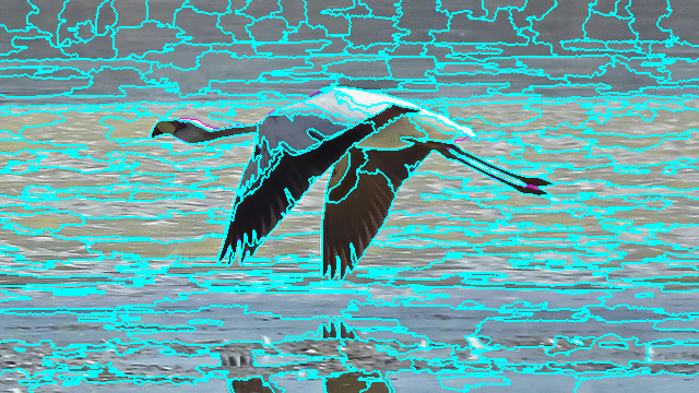
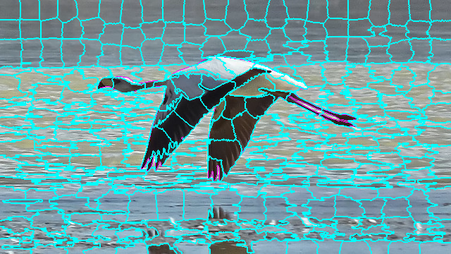
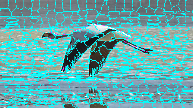
(a)	(b)	(c)

Figure 1: Superpixel segmentation with the same input number (300) of regions for (a) an ISF method, (b) SLIC, and (c) LSC. The borders of the superpixels (cyan) overlap the ground-truth borders (magenta) — i.e., errors appear in magenta.

In this paper, we propose an Iterative Spanning Forest (ISF) framework for generating connected superpixels with no overlap, conforming to a hard segmentation. Our framework is based on sequences of Image Foresting Transforms (IFTs) [11] and has four components, namely, i) a seed sampling strategy, ii) a connectivity function, iii) an adjacency relation, and iv) a seed recomputation procedure. Each iteration of the ISF algorithm executes one IFT from a distinct seed set, yielding to a sequence of segmentation results that improve along the iterations until convergence. In order to illustrate the framework, we present i) a mixed seed sampling strategy based on normalized Shannon entropy, the standard grid sampling, and a regional-minima-based sampling; ii) three connectivity functions; iii) two adjacency relations, 4-neighborhood in 2D and 6-neighborhood in 3D; and iv) two seed recomputation procedures. The mixed sampling strategy aims at estimating higher number of seeds in more heterogeneous regions in order to improve boundary adherence. Grid sampling tends to produce more regularly distributed superpixels and the regional-minima-based strategy aims at solving superpixel segmentation in a single IFT iteration. Two connectivity functions allow to control the balance between boundary adherence and superpixel regularity, and the third one maximizes boundary adherence regardless to superpixel regularity. Both adjacency relations guarantee the connectivity between pixels and their corresponding seeds (i.e., a result consistent with the superpixel definition). For seed recomputation, we present procedures that exploit color and spatial information, and color information only. At each iteration, the IFT algorithm propagates paths from each seed to pixels that are more closely connected to that seed than to any other, according to a given connectivity function. The resulting superpixels are spanning trees rooted at those seeds.

Boundary adherence and superpixel regularity are inversely related properties. Some works have mentioned the importance of superpixel regularity — i.e., of obtaining compact [12] and regularly distributed [13, 14] superpixels. However, the need for superpixel regularity in high level applications requires a more careful study. Given that the image objects must be represented by the union of its superpixels, boundary adherence is certainly the most important property. Figure 1 shows segmentation results with the same input number (300) of superpixels for one of the ISF methods, SLIC (Simple Linear Iterative Clustering) [1], and LSC (Linear Spectral Clustering) [15]. Note that ISF can preserve more accurately the object borders as compared to SLIC and LSC.

For validation, we first select four 2D image datasets that represent scenarios with distinct characteristics. The ISF methods are compared with five approaches from the state-of-the-art: SLIC [1], LSC [15], ERS (Entropy Rate Superpixel) [16], LRW (Lazy Random Walk) [17], and Waterpixels [18]. We also add a hybrid approach that combines ISF with the fastest among them, SLIC. Effectiveness is evaluated by plots with varying number of superpixels of the most commonly used boundary adherence measures in superpixel segmentation: Boundary Recall (BR), as implemented in [1], and Undersegmentation Error (UE), as implemented in [19]. Since SLIC is the only baseline with 3D implementation, we compare the effectiveness of ISF, SLIC, and the hybrid SLIC-ISF on the 3D segmentation of three objects — left brain hemisphere, right brain hemisphere, and cerebellum — from volumetric MR (Magnetic Resonance) images. This experiment uses the most effective ISF method for this application and effectiveness is measured by f-score for three segmentation resolutions (low, medium, and high numbers of supervoxels). Another experiment involves a high level application, named sky image segmentation, in which the label assignment to the superpixels is decided by an independent and automatic algorithm. We measure the f-score for varying number of superpixels using SLIC (the fastest baseline), LSC (the most competitive baseline), and the most effective ISF method for this application. For efficiency evaluation, we compare the processing time for varying number of superpixels among one of the ISF methods, SLIC-ISF, SLIC, and the two most competitive baselines in effectiveness, LSC and ERS.

In Section II, we discuss the related works. The ISF framework and five ISF methods are presented in Section III. In this section, we also present the general ISF algorithm, discusses implementation issues, and provide the link for its code. Section IV presents the experimental results and the ISF theoretical properties are demonstrated in the supplementary material. Section V states conclusion and discusses future work.

II Related Work

Most superpixel segmentation approaches adopt a clustering algorithm and/or a graph-based algorithm to address the problem in one or multiple iterations of seed estimation. Several of these methods cannot guarantee connected superpixels: SLIC (Simple Linear Interative Clustering) [1], LSC (Linear Spectral Clustering) [15], Vcells (Edge-Weighted Centroidal Voronoi Tessellations) [20], LRW (Lazy Random Walks) [17], ERS (Entropy Rate Superpixels) [16], and DBSCAN (Density- based spatial clustering of applications with noise) [21]. Connected superpixels in these methods are usually obtained by merging regions, as a post-processing step, which can reduce the number of desired superpixels.

Some representative graph-based algorithms include Normalized Cuts [13], an approach based on minimum spanning tree [22], a method using optimal path via graph cuts [14], an energy minimization framework which can also yield supervoxels [23], the watershed transform from seeds [24, 25, 18], and approaches based on random walk [16, 17]. Normalized cuts can generate more compact and more regular superpixels. However, as shown in [1], it performs below par in boundary adherence with respect to other methods. The problem with the algorithm in [22] is exactly the opposite. The resulting superpixels can conform to object boundaries, but they are very irregular in size and shape. Similar effect happens in these graph-based watershed algorithms [24, 25]. An exception is the waterpixel approach [18] that enforces compactness by using a modified gradient image. However, these algorithms try to solve the segmentation problem from a single seed set (e.g., seeds are selected from the regional minima of a gradient image). Due to the absence of seed recomputation and/or quality of the image gradient, they usually miss important object boundaries. The performance of the method described in [14] depends on the pre-computed boundary maps, which is not guaranteed to be the best in all cases. The authors in [23] actually suggest two methods for generating compact and constant-intensity superpixels. In [16], the authors use entropy rate of a random walk on a graph and a balancing term for superpixel segmentation. The method yields good segmentation results, but it involves a greedy strategy for optimization. In [17], the authors show that the lazy random walk produces better results, but the method has initialization and optimization steps, both requiring the computation of the commute time, which tends to adversely affect the total execution time.

ISF falls in the category of graph-based algorithms as a particular case of a more general framework [11] — the Image Foresting Transform (IFT). The IFT is a framework for the design of image operators based on connectivity, such as distance and geodesic transforms, morphological reconstructions, multiscale skeletonization, image description, region- and boundary-based image segmentation methods [26, 24, 27, 28, 29, 30, 31, 32, 33], with extensions to clustering and classification [34, 35, 36, 37, 38]. As discussed in [39], by choice of the connectivity function, the IFT algorithm computes a watershed transform from a set of seeds that corresponds to a graph cut in which the minimum gradient value in the cut is maximized. From [25], it is known that the watershed transform from seeds is equivalent to a cut in a minimum-spanning tree (MST). That is, the removal of the arc with maximum weight from the single path in the MST that connects each pair of seeds results a minimum-spanning forest (i.e., a watershed cut). Such a graph cut tends to be better than the normalized cut in boundary adherence, but worse in superpixel regularity.

In the evolution of superpixel segmentation methods, it is also worth mentioning Mean-Shift [40], Quick-Shift [41], turbopixels [42], SLIC [1], geometric flow [43], LSC [15], and DBSCAN [21]. The Mean-Shift method produces irregular and loose superpixels whereas the Quick-Shift algorithm does not allow an user to choose the number of superpixels. The turbopixel-based approaches can produce good superpixels, but are computationally complex. Çi$\check{\rm g}$la and Atalan [44] used connected k-means algorithm with convexity constraints to achieve superpixel segmentation via speeded-up turbopixels. The method is still bit slow, and, as claimed by the authors, fails to provide good boundary recall for complex images. SLIC is by far the most commonly used superpixel method [1]. It uses a regular grid for seed sampling. Once chosen, the seeds are transferred to the lowest gradient position within a small neighborhood. Finally, a modified k-means algorithm is used to cluster the remaining pixels. This algorithm was shown to perform better than many other methods (e.g., [42, 13, 22, 23, 41]). However, the k-means algorithm searches for pixels within a $2S\times 2S$ window around each seed, where $S$ is the grid interval. For a non-regular seed distribution, some pixels may not be reached by any seed. Indeed, this might happen from the second iteration on and this labeling inconsistency problem is only solved by post-processing. In [43], Wang et al. proposed a geometric-flow-based method of superpixel generation. The method has high computational complexity as it involves computation of the geodesic distance and several iterations. LSC [15] and DBSCAN [21] are among the most recent approaches. LSC models the segmentation problem using Normalized Cuts, but it applies an efficient approximate solution using a weighted k-means algorithm to generate superpixels. DBSCAN performs fast pixel grouping based on color similarity with geometric restrictions, and then merges small clusters to ensure connected superpixels.

A first method based on the ISF framework appeared in [45] and has been successfully used in a high level application [33]. It is considered in our experiments.

III The ISF framework

An ISF method results from the choice of each component: inital seed selection, connectivity function, adjacency relation, and seed recomputation strategy. The ISF algorithm is a sequence of Image Foresting Transforms (IFTs) from improved seed pixel sets (Section III-A). For initial seed selection, we propose either grid or mixed entropy-based seed sampling as effective strategies (Section III-B). The closest minima of a gradient image to seeds obtained by grid sampling is also evaluated in an attempt to solve the problem in a single iteration. Examples of connectivity functions and adjacency relations for 2D and 3D segmentations are presented in Sections III-C and III-D, respectively. Two strategies for seed recomputation are described in Section III-E. The ISF algorithm is presented in Section III-G and its theoretical properties are demonstrated in the supplementary material. Section III-H discusses implementation issues and provides the link to the code.

III-A Image Foresting Transform

An image can be interpreted as a graph $G=({\cal I},{\cal A})$, whose pixels in the image domain ${\cal I}\subset Z^{n}$ are the nodes and pixel pairs $(s,t)$ that satisfy the adjacency relation ${\cal A}\subset{\cal I}\times{\cal I}$ are the arcs (e.g., $4$-neighbors when $n=2$). We use $t\in{\cal A}(s)$ and $(s,t)\in{\cal A}$ to indicate that $t$ is adjacent to $s$.

For a given image graph $G=({\cal I},{\cal A})$, a path $\pi_{t}=\langle t_{1},t_{2},\ldots,t_{n}=t\rangle$ is a sequence of adjacent pixels with terminus $t$. A path is trivial when $\pi_{t}=\langle t\rangle$. A path $\pi_{t}=\pi_{s}\cdot\langle s,t\rangle$ indicates the extension of a path $\pi_{s}$ by an arc $(s,t)$. When we want to explicitly indicate the origin of a path, the notation $\pi_{s\leadsto t}=\langle t_{1}=s,t_{2},\ldots,t_{n}=t\rangle$ is used, where $s$ stands for the origin and $t$ for the destination node. A predecessor map is a function $P$ that assigns to each pixel $t$ in ${\cal I}$ either some other adjacent pixel in ${\cal I}$, or a distinctive marker $nil$ not in ${\cal I}$ — in which case $t$ is said to be a root of the map. A spanning forest (image segmentation) is a predecessor map which contains no cycles — i.e., one which takes every pixel to $nil$ in a finite number of iterations. For any pixel $t\in{\cal I}$, a spanning forest $P$ defines a path $\pi_{t}^{P}$ recursively as $\langle t\rangle$ if $P(t)=nil$, and $\pi_{s}^{P}\cdot\langle s,t\rangle$ if $P(t)=s\neq nil$.

A connectivity (path-cost) function computes a value $f(\pi_{t})$ for any path $\pi_{t}$, including trivial paths $\pi_{t}=\langle t\rangle$. A path $\pi_{t}$ is optimum if $f(\pi_{t})\leq f(\tau_{t})$ for any other path $\tau_{t}$ in $\Pi_{G}$ (the set of paths in $G$). By assigning to each pixel $t\in{\cal I}$ one optimum path with terminus $t$, we obtain an optimal mapping $C$, which is uniquely defined by $C(t)=\min_{\forall\pi_{t}\;\text{in}\;\Pi_{G}}\{f(\pi_{t})\}$. The Image Foresting Transform (IFT) [11] takes an image graph $G=({\cal I},{\cal A})$, and a connectivity function $f$; and assigns one optimum path $\pi_{t}$ to every pixel $t\in{\cal I}$ such that an optimum-path forest $P$ is obtained — i.e., a spanning forest where all paths are optimum. However, $f$ must satisfy certain conditions, as described in [46], otherwise, the paths may not be optimum.

In ISF, all seeds are forced to be the roots of the forest by choice of $f$, in order to obtain a desired number of superpixels. For any given seed set ${\cal S}$, each superpixel will be represented by its respective tree in the spanning forest $P$ as computed by the IFT algorithm.

III-B Seed Sampling Strategies

Any natural image contains a lot of heterogeneity. Some parts of the image can have really small variations in intensity whereas some parts in the image can show significant variations. So, it is but natural to choose more seeds from a more non-uniform region of an image. However, having a grid structure for the seeds is also essential to conform to the regularity of the superpixels. The proposed mixed sampling strategy achieves both the goals. We use a two-level quad-tree representation of an input 2D image. The heterogeneity of each quadrant (Q) is captured using Normalized Shannon Entropy (NSE(Q)). This is given by

$$NSE(Q)=-\frac{\sum_{i=1}^{n}{p_{i}}{log_{2}(p_{i})}}{log_{2}n}.$$ (1)

Here $n$ denotes the total number of intensity levels in the quadrant Q and $p_{i}$ is the probability of occurrence of the intensity $i$ in the quadrant Q. For color images, we deem the lightness component in the Lab color model as the intensity of a pixel. Normalizing the entropy ensures that the $NSE(Q)\in[0,1]$. At the first level in the quad-tree, we compute the normalized Shannon entropies for each quadrant and also obtain the mean $\mu(NSE)$ and the standard deviation $\sigma(NSE)$ of the four values. If the value of entropy for any quadrant exceeds the mean by one standard deviation, i.e., if $|NSE(Q)-\mu(NSE)|>\sigma(NSE)$, then we further divide the region in the next level into four quadrants. We then compute the NSE values for the new quadrants at the second level. Once, the two-level quad-tree representation is complete, we assign the number of seeds to be selected from each region as proportional to their NSE values. Finally, the seeds from each region are picked based on the grid sampling strategy. So, we essentially perform local grid sampling for each leaf node in the two-level quad-tree. This procedure may improve boundary recall with respect to grid sampling, depending on the dataset. In addition to grid and mixed sampling strategies, we have also evaluated seed selection based on the reduction of the seed set generated by grid sampling to the set of the closest regional minima in a gradient image.

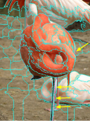
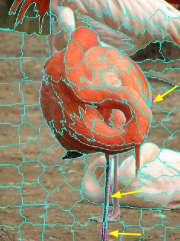
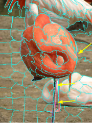
(a)	(b)	(c)	(d)	(e)

Figure 2: Segmentation results of an image from Birds [47] for five ISF methods (a) ISF-GRID-ROOT (BR = 0.93, UE = 0.01), (b) ISF-MIX-ROOT (BR = 0.89, UE = 0.02), (c) ISF-GRID-MEAN (BR = 0.90, UE = 0.02), (d) ISF-MIX-MEAN (BR = 0.86, UE = 0.02), and (e) ISF-REGMIN (BR = 0.82, UE = 0.02). Yellow arrows indicate leaking between object and background.

III-C Connectivity Functions

We consider the computation of the IFT with two path-cost functions that only guarantee a spanning forest, $f_{1}$ (Equation 5) and $f_{2}$ (Equation 6), and a third one, $f_{3}$ (Equation 7), that guarantees an optimum-path forest. The spanning forest in $f_{1}$ and $f_{2}$ might not be optimum, because the path costs depend on path-root properties [46]. However, these functions can efficiently deal with the problem of intensity heterogeneity [27].

The seed sampling approach (e.g. grid or mixed) defines an initial seed set ${\cal S}$, such that for each seed pixel $s_{j}\in{\cal S}$ at coordinate $(x_{j},y_{j})$, its color representation in the Lab color space is given $I(s_{j})=[l_{j}\;a_{j}\;b_{j}]^{T}$. A path-cost function $f$ is defined by a trivial-path cost initialization rule and an extended-path cost assignment rule. We present three instances of $f$, denoted as $f_{1}$, $f_{2}$ and $f_{3}$, with trivial-path initialization rule given by

$$f_{\ast}(\pi_{t}=\langle t\rangle) = \left\{\begin{array}[]{ll}0&\mbox{if $t\in{\cal S}$,}\\ +\infty&\mbox{otherwise.}\end{array}\right.$$ (4)

They differ in the extended-path cost assignment rule, as follows.

$$f_{1}(\pi_{s_{j}\leadsto s}\cdot\langle s,t\rangle)=f_{1}(\pi_{s})+\left(\|I(t)-I(s_{j})\|\alpha\right)^{\beta}+\|s,t\|,$$ (5)

where $\alpha\geq 0$, $\beta\geq 1$, and $I(t)=[l_{t}\;a_{t}\;b_{t}]^{T}$ is the color vector at pixel $t$.

$$f_{2}(\pi_{s_{j}\leadsto s}\cdot\langle s,t\rangle)=f_{2}(\pi_{s})+\left(\|I(t)-M(s_{j})\|\alpha\right)^{\beta}+\|s,t\|,$$ (6)

where $M(s_{j})$ is the mean color, computed inside the superpixel of the previous iteration, which contains the new seed $s_{j}$ ($M(s_{j})=I(s_{j})$ at the first iteration).

$$f_{3}(\pi_{r\leadsto s}\cdot\langle s,t\rangle)=\max\{f_{3}(\pi_{s}),D(t)\},$$ (7)

where $D(t)$ is the value of the gradient image in the pixel $t$.

At the end of the IFT algorithm, each superpixel will be represented by its respective tree in the spanning forest $P$. After that, an update step adjusts the roots (new seeds) of the spanning trees.

For paths $\pi_{t_{1}\leadsto t_{n}}=\langle t_{1},t_{2},\ldots,t_{n}\rangle$, $n>1$, and additive path-cost function $f(\pi_{t_{1}\leadsto t_{n}})=\sum_{i=1,2,\ldots,n-1}\{w(t_{i},t_{i+1})\}$, $w(t_{i},t_{i+1})\geq 0$, the minimization of the cost map imposes too much shape regularity on superpixels, by avoiding adherence to image boundaries. On the other hand, $f(\pi_{t_{1}\leadsto t_{n}})=\max_{i=1,2,\ldots,n-1}\{w(t_{i},t_{i+1})\}$ (Equation 7, for $w(t_{i},t_{i+1})=D(t_{i+1})$) provokes high adherence to image boundaries, but also possible leakings when delineating poorly defined parts of the boundaries. The path-cost function $f(\pi_{t_{1}\leadsto t_{n}})=\sum_{i=1,2,\ldots,n-1}\{w(t_{i},t_{i+1})^{\beta}\}$, $\beta>1$, represents a compromise between the previous two. We fix $\beta=12$ in all experiments to approximate the effect of high adherence to image boundaries with considerably reduced leaking in superpixel segmentation. The arc weight $w(t_{i},t_{i+1})=\|I(t_{i+1})-I(s_{j})\|\alpha$ (Equation 5 for $s_{j}=t_{1}$), or $w(t_{i},t_{i+1})=\|I(t_{i+1})-M(s_{j})\|\alpha$ (Equation 6 for $s_{j}=t_{1}$), penalizes paths that cross image boundaries, but the choice of $\alpha$ provides the compromise between the shape regularity on superpixels, as imposed by the spatial connectivity component $\|t_{n-1},t_{n}\|$ in Equations 5 and 6, and the high boundary adherence of $\sum_{i=1,2,\ldots,n-1}\{w(t_{i},t_{i+1})^{\beta}\}$ for $\beta=12$. The choice of $\alpha$ is then optimized to maximize performance in BR and UE, without compromising too much the regularity of the superpixels (as it happens with $f_{3}$).

III-D Adjacency Relation

The popular choices for adjacency relation are 4- or 8-neighborhood in 2D and 6- or 26-neighborhood in 3D in order to ensure connected superpixels (supervoxels). We prefer simple symmetric adjacency of 4-neighborhood in 2D and 6-neighborhood in 3D. This choice helps in the regularity of the superpixels/supervoxels.

III-E Seed Recomputation

We next discuss the automated seed recomputation strategy. Let $s_{i}^{t}$ be the $i^{th}$ superpixel root (seed) at iteration $t$ and its feature vector defined as $[l_{i}^{t}\;a_{i}^{t}\;b_{i}^{t}\;x_{i}^{t}\;y_{i}^{t}]^{T}$. We select $s_{i}^{t}$ either as the pixel of the superpixel whose color is the most similar to the mean color of the superpixel or as the pixel of the superpixel that is the closest to its geometric center. During the subsequent IFT computations, we only recompute the seed $s_{i}^{t+1}$ if:

$$\|[l_{i}^{t}\;a_{i}^{t}\;b_{i}^{t}]-[l_{i}^{t+1}\;a_{i}^{t+1}\;b_{i}^{t+1}]\|>\sqrt{\mu_{c}}$$ (8)

or

$$\|[x_{i}^{t}\;y_{i}^{t}]-[x_{i}^{t+1}\;y_{i}^{t+1}]\|>\sqrt{\mu_{s}},$$ (9)

where $\mu_{c}$ and $\mu_{s}$ are the average color and spatial distances to seed $s_{i}^{t}$.

III-F Five Different ISF Methods

We present five ISF methods. The first two use function $f_{1}$, ISF-GRID-ROOT is based on grid sampling and ISF-MIX-ROOT is based on mixed sampling. They recompute seeds as the pixel inside each superpixel whose color is the closest to the mean color of the superpixel. The third and fourth methods use function $f_{2}$, ISF-GRID-MEAN is based on grid sampling and ISF-MIX-MEAN is based on mixed sampling. They recompute seeds as the pixel inside each superpixel whose position is the closest to the geometric center of the superpixel. In [45], we presented ISF-GRID-MEAN.

We now discuss the fifth superpixel generation method, called ISF-REGMIN, that uses the path-cost function $f_{3}$. ISF-REGMIN is designed to be fast, as it uses only a single iteration of the IFT algorithm with no seed recomputation. This method initially performs grid sampling to set the seeds. Then, the seeds are substituted by any pixel at the closest regional minimum, computed in the gradient image.

It is important to note that the ISF methods do not require a post-processing step as the connectivity is already guaranteed by design.

Figure 2 presents the segmentation results of the five ISF methods on an image of Birds [47]: ISF-GRID-ROOT, ISF-MIX-ROOT, ISF-GRID-MEAN, ISF-MIX-MEAN and ISF-REGMIN. For this dataset, with thin and elongated object parts, ISF-GRID-ROOT obtains the best result. However, ISF-MIX-MEAN performs better on most datasets.

III-G The ISF Algorithm

Algorithm 1 presents the Iterative Spanning Forest procedure.

Algorithm 1.

– Iterative Spanning Forest
Input: Image $\hat{I}=({\cal I},I)$, adjacency relation ${\cal A}$, initial seed set ${\cal S}\subset{\cal I}$, the parameters $\alpha\geq 0$ and $\beta\geq 1$, and the maximum number of iterations $MaxIters\geq 1$. Output: Superpixel label map $L_{s}$. Auxiliary: State map $S$, priority queue $Q$, predecessor map $P$, cost map $C$, root map $R$ and superpixel mean color array $M$.

1.	$iter\leftarrow 0$
2.	While $iter<MaxIter$, do
3.			For each $t\in{\cal I}$, do
4.					$P(t)\leftarrow nil$, $R(t)\leftarrow t$
5.					$S(t)\leftarrow White$, $C(t)\leftarrow+\infty$
6.			$label\leftarrow 1$
7.			For each $t\in{\cal S}$, do
8.					$C(t)\leftarrow 0$
9.					$L_{s}(t)\leftarrow label$, $label\leftarrow label+1$
10.					Insert $t$ in $Q$, $S(t)\leftarrow Gray$
11.					If $iter=0$, then
12.							$M(t)\leftarrow I(t)$
13.			While $Q\neq\emptyset$, do
14.					Remove $s$ from $Q$ such that $C(s)$ is minimum
15.					$S(s)\leftarrow Black$
16.					For each $t\in{\cal A}(s)$, such that $S(t)\neq Black$ , do
17.							$c\leftarrow C(s)+\left(\|I(t)-M(R(s))\|\alpha\right)^{\beta}+\|s,t\|$
18.							If $c<C(t)$, then
19.									Set $P(t)\leftarrow s$, $R(t)\leftarrow R(s)$
20.									Set $C(t)\leftarrow c$, $L_{s}(t)\leftarrow L_{s}(s)$
21.									If $S(t)=Gray$, then
22.											Update position of $t$ in $Q$
23.									Else
24.											Insert $t$ in $Q$
25.											$S(t)\leftarrow Gray$
26.			${\cal S},M\leftarrow RecomputeSeeds({\cal S},\hat{I},L_{s})$
27.			$iter\leftarrow iter+1$
28.	Return $L_{s}$

Line 1 initializes the auxiliary variable $iter$ (iteration number). The loop in Line 2 stops when the maximum number of iterations is achieved. Lines 3-5 initialize the values for the predecessor, root, state and cost maps for all image pixels. The state map $S$ indicates by $S(t)=White$ that a pixel $t$ was never visited (never inserted in the priority queue $Q$), by $S(t)=Gray$ that $t$ has been visited and is still in $Q$, and by $S(t)=Black$ that $t$ has been processed (removed from $Q$). Lines 7-12 initialize the cost and label maps and insert the seeds in $Q$. The seeds are labeled with consecutive integer numbers in the superpixel label map $L_{s}$. Lines 13-25 perform the label propagation process. First, we remove the pixels $s$ that have minimum path cost in $Q$. Then the loop in Lines 16-25 evaluates if a path with terminus $s$ extended to its adjacent $t$ is cheaper than the current path with terminus $t$ and cost $C(t)$. If that is the case, $s$ is assigned as the predecessor of $t$ and the root of $s$ is assigned to the root of $t$ (Line 19). The path cost and the label of $t$ are updated. If $t$ is in $Q$, its position is updated, otherwise $t$ is inserted into $Q$. After the label propagation stage, function $RecomputeSeeds$ returns the new seed set and the new mean color values $M$ for the superpixels. Note that in the first iteration the feature vector of the superpixel root is the seed pixel color (Line 11-12). The tasks of label propagation and seed recomputation are performed until the condition of Line 2 is achieved. The algorithm returns the label map $L_{s}$ (superpixel segmentation). Note that the algorithm describes the method ISF-MIX-MEAN if we use mixed sampling as seed initialization strategy. It uses the path-cost function $f_{2}$ (see Equation 6) in Line 17. By replacing Line 17 with the path-cost function $f_{1}$ (see Equation 5), we obtain the algorithm for the method ISF-MIX-ROOT. Finally, by replacing mixed sampling by grid sampling in ISF-MIX-ROOT, we obtain the method ISF-GRID-ROOT.

III-H Implementation issues and available code

In general, using a priority queue as a binary heap, each execution of the IFT algorithm takes time $O(N\log N)$ for $N=|{\cal I}|$ pixels (linearithmic time). Given that the time to recompute seeds is linear, the complexity of the ISF framework using a binary heap is linearithmic, independently of the number of superpixels. For integer path costs, such as in ISF-REGMIN, it is possible to reduce the IFT execution time to $O(N)$ using a priority queue based on bucket sorting [26].

For efficient implementation, we use a new variant, as proposed in  [48], of the Differential Image Foresting Transform (DIFT) algorithm [49]. This algorithm is able to update the spanning forest by revisiting only pixels of the regions modified in a given iteration $iter>1$. The efficient implementation of ISF is available at www.ic.unicamp.br/~afalcao/downloads.html.

IV Experimental Results

In this section, we evaluate the methods based on effectiveness in 2D and 3D image datasets, effectiveness in a high level application, and efficiency.

IV-A Effectiveness in 2D and 3D datasets

We first measure the effectiveness of the methods in Boundary Recall (BR) (as implemented in [1]) and Undersegmentation Error (UE) (as implemented in [19]) using plots with varying number of superpixels on four 2D datasets: Berkeley [50] (300 natural images), Birds [47] (50 natural images), Grabcut [51] (50 natural images), and Liver (50 CT slice images of the abdomen). The objects in Birds are fine and elongated structures and the images of the liver are grayscale.

The ISF methods are compared with five approaches from the state-of-the-art: SLIC (Simple Linear Interative Clustering) [1] , LSC (Linear Spectral Clustering) [15] , ERS (Entropy Rate Superpixel) [16], LRW (Lazy Random Walk) [17] , and Waterpixels [18]. Except for ISF-REGMIN, the remaining ISF methods are competitive among themselves with some differences in effectiveness. Therefore, in order to avoid busy and confusing plots, we present the effectiveness of two of the best ISF methods (10 iterations), ISF-GRID-ROOT and ISF-MIX-MEAN, for each dataset. We maintain ISF-REGMIN in the plots, because it (a) uses an integer path cost function, which allows fast computation in time proportional to the number of pixels and independent of the number of seeds (superpixels), (b) does not require seed recomputation, and even being the simplest among the ISF methods, (c) it shows consistently better effectiveness than its counterpart, Waterpixels [18]. We also include a fast hybrid approach, namely SLIC-ISF, that combines 10 iterations of SLIC for seed estimation, followed by 2 iterations of ISF, to show that it is competitive with the other ISF methods in most datasets. Figures 3–6 show the results of this first round of experiments, using $\alpha=0.5$ and $\beta=12$ for the ISF methods that use $f_{1}$ or $f_{2}$.

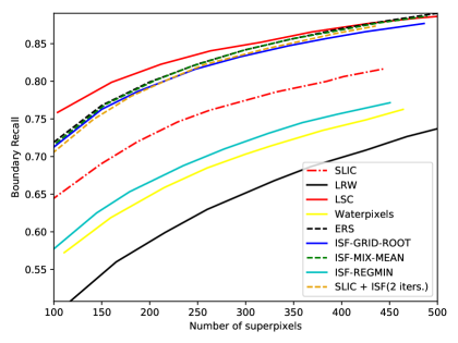
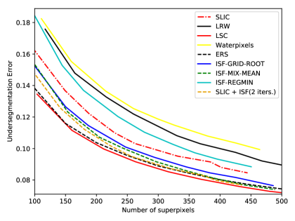
Figure 3: Variations of BR, UE with number of superpixels for ISF-MIX-MEAN, ISF-GRID-ROOT, ISF-REGMIN, SLIC, the combination of SLIC and ISF (two iterarions), LRW, ERS, Waterpixels and LSC methods on Berkeley. We use the parameters $\alpha=0.5$ for ISF variants, $m=10$ (compactness parameter) for SLIC variants, $\alpha=0.999999$ for LRW, $k=8$ for Waterpixels and $ratio=0.075$ for LSC.

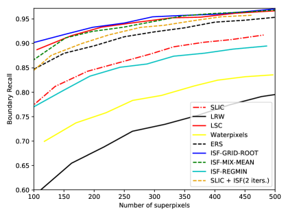
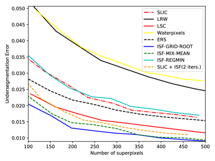
Figure 4: Variations of BR, UE with number of superpixels for ISF-MIX-MEAN, ISF-GRID-ROOT, ISF-REGMIN, SLIC, the combination of SLIC and ISF (two iterarions), LRW, ERS, Waterpixels and LSC methods on Birds. We use the parameters $\alpha=0.5$ for ISF variants, $m=10$ (compactness parameter) for SLIC variants, $\alpha=0.999999$ for LRW, $k=8$ for Waterpixels and $ratio=0.075$ for LSC.

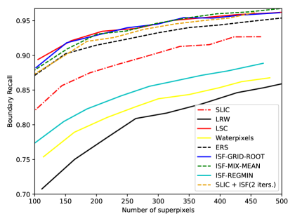
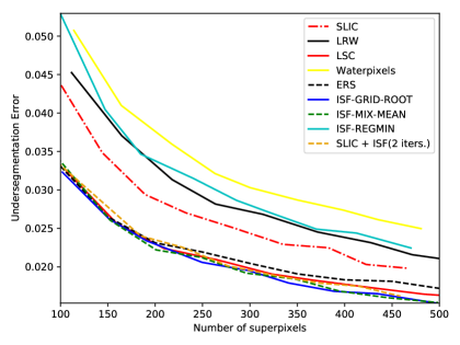
Figure 5: Variations of BR, UE with number of superpixels for ISF-MIX-MEAN, ISF-GRID-ROOT, ISF-REGMIN, SLIC, the combination of SLIC and ISF (two iterarions), LRW, ERS, Waterpixels and LSC methods on Grabcut. We use the parameters $\alpha=0.5$ for ISF variants, $m=10$ (compactness parameter) for SLIC variants, $\alpha=0.999999$ for LRW, $k=8$ for Waterpixels and $ratio=0.075$ for LSC.

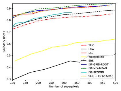
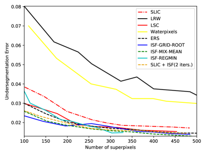
Figure 6: Variations of BR, UE with number of superpixels for ISF-MIX-MEAN, ISF-GRID-ROOT, ISF-REGMIN, SLIC, the combination of SLIC and ISF (two iterarions), LRW, ERS, Waterpixels and LSC methods on Liver. We use the parameters $\alpha=0.5$ for ISF variants, $m=10$ (compactness parameter) for SLIC variants, $\alpha=0.999999$ for LRW, $k=8$ for Waterpixels and $ratio=0.075$ for LSC.

Although LSC presents the best performance (the highest BR and the lowest UE) in Berkeley, the same is not observed in the other three datasets. For Birds, Grabcut, and Liver, the best methods are ISF-GRID-ROOT, ISF-GRID-ROOT (being equivalent to ISF-MIX-MEAN), and ISF-MIX-MEAN, respectively. In Berkeley, ISFMIX-MEAN performs second best in BR and SLIC-ISF performs second best in UE. ISF-REGMIN is consistenly better than Waterpixels in both BR and UE for all datasets. ERS performs well in Berkeley, but its performance is not competitive in the other three datasets. Although SLIC is the fastest and most used method, its performance is far from being competitive in all datasets. Among the baselines, LSC is the most competitive with the ISF methods. However, it seems that the performance of LSC in UE can be negatively affected for thin and elongated objects, such as birds. Except for Berkeley, SLIC-ISF presents better performance than ERS in BR and UE.

In conclusion, one cannot say that there is a winner for all datasets, but it is clear that ISF can produce highly effective methods with different performances depending on the dataset. In Birds, Grabcut, and Liver, ISF shows better effectiveness than the most competitive baseline, LSC. This shows the importance of obtaining connected superpixels with no need for post-processing. The performance of LSC in UE is usually inferior when compared to its performance in BR. Birds dataset is clearly a case in the point. Indeed, LSC produces less regular superpixels with high BR. In sky image segmentation, as we will see, this property of LSC considerably impairs its effectiveness. Between ISF-GRID-ROOT and ISF-MIX-MEAN, we can say that ISF-MIX-MEAN provides better results in most datasets, including the application of sky image segmentation. We believe this is related to the advantages in effectiveness of mix sampling over grid sampling. Figure 7 then illustrates the quality of the segmentation in images from three datasets using the best ISF method for the dataset, the fastest approach, SLIC, and the most competitive baseline, LSC. Additionaly, we show the ISF method with a choice of $\alpha=0.12$ that produces more regular superpixels without compromising its performance in BR and UE. This simply shows that by choice of $\alpha$, ISF can control superpixel regularity.

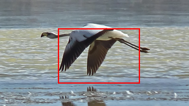
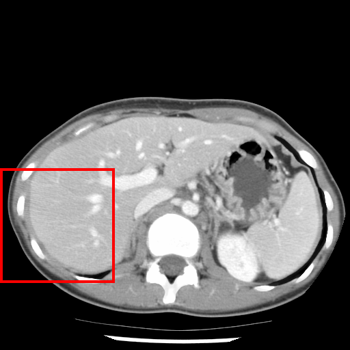
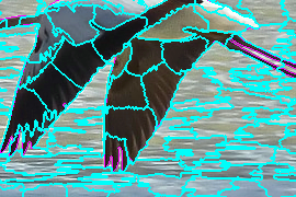
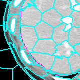
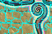
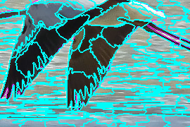
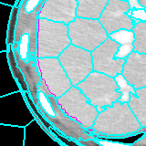
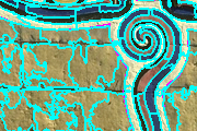
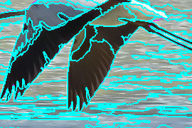
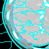
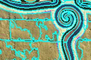
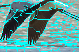
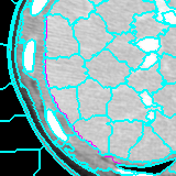
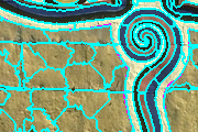
(a)	(b)	(c)

Figure 7: Examples of superpixel segmentation in (a) Birds, (b) Liver and (c) Berkeley, using SLIC (second row), LSC (third row), ISF with $\alpha=0.5$ (fourth row), and ISF with $\alpha=0.12$ (fifth row) — ISF-GRID-ROOT (first column), ISF-MIX-MEAN (second column), and ISF-MIX-MEAN (third column). The superpixel borders are presented in cyan and the ground-truth borders in magenta (i.e., errors appear in magenta).

Second, given that the 3D extension of ISF simply requires a different choice of adjacency relation, we present a comparison between the best ISF method for this application (ISF-GRID-MEAN with $\alpha=0.1$), the only baseline with 3D implementation (SLIC), and the hybrid approach (SLIC-ISF) on volumetric MR images of the brain. In this dataset, there are three objects of interest: cerebellum, left and right brain hemispheres (Figure 8a). Segmentation creates supervoxels as shown in Figure 8b. Supervoxels with more than 50% of their voxels inside a particular object are labeled as belonging to that object, otherwise they are considered as part of the background or other objects. Effectiveness is measured by f-score for three supervoxel resolutions, given the usual image sizes: low ($N=1000$), medium ($N=5000$), and high ($N=10000$). Table I shows the results of this experiment, using a 64 bit, Core(TM) i7-3770K Intel(R) PC with CPU speed of 3.50GHz. It is not a surprise that ISF outperforms SLIC in effectiveness. However, SLIC is exploiting parallel computing  and given that SLIC-ISF is twice faster than ISF, their equivalence in performance above medium superpixel resolution is an excellent result. Another interesting observation is that ISF performs better for a value of $\alpha$ ($\alpha=0.1$) lower than $0.5$ (i.e., more regular supervoxels).

TABLE I: Fscore (mean +/- std. deviation) for cerebellum, left and right brain hemispheres in 3D MR images.

	$N=1000$			$N=5000$			$N=10000$
Method	FScore	Stdev	Time(sec)	FScore	Stdev	Time(sec)	FScore	Stdev	Time(sec)
SLIC	0.8584	0.0110	6.1	0.9194	0.0075	7.0	0.9369	0.0039	7.2
ISF-GRID-MEAN	0.8815	0.0129	31.8	0.9321	0.0069	30.3	0.9459	0.0051	29.9
SLIC + ISF (two iterations)	0.8686	0.0138	17.3	0.9305	0.0072	18.0	0.9444	0.0044	18.0

Figures 8c-d show another example using ISF-GRID-MEAN, where the specification of 10 supervoxels using $\alpha=0.5$ segments the patella bone as one of the supervoxels.

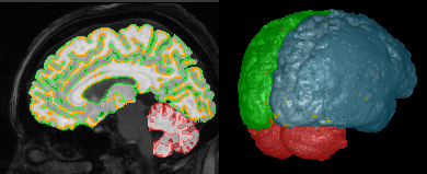
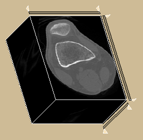
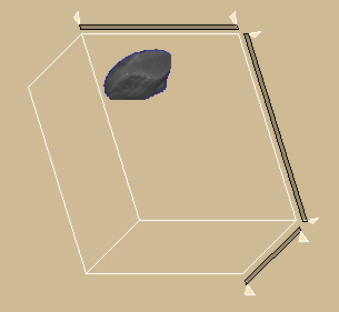
Figure 8: (a) Cerebellum, left and right brain hemispheres from an MR image of the brain. (b) Resulting supervoxels for one MR image of the brain. (c) CT image of a knee. (d) For a segmentation of 10 supervoxels, the patella bone is obtained as one of them.

IV-B Effectiveness in a high level application

When considering a high level application, such as superpixel-based image segmentation, the label assigment to superpixels follows some independent and automatic rule. In this section, we evaluate the performance of the best ISF method (ISF-MIX-MEAN) in this application, namely sky image segmentation, in comparison with the fastest method (SLIC) and the most competitive baseline (LSC). We use a simple yet effective sky segmentation algorithm, as presented in [3]. This algorithm uses the mean color of the superpixels and a threshold defined in the Lab color space to merge superpixels. The region (set of superpixels) in the top of the image that contains the larger number of pixels is selected as the sky region. Figure 9 shows the results of f-score for this experiment for varying number of superpixels. Again, ISF with $\alpha=0.08$ (more regular superpixels) performs better than the others.

The use of lower values of $\alpha$ in the segmentation of 3D MR images of the brain and in this application strongly suggests that superpixel regularity has some importance as well as boundary adherence. It is also interesting to observe that SLIC outperforms LSC in this application.

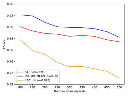
Figure 9: Performance in f-score (Dice) for sky image segmentation: ISF-MIX-MEAN, SLIC, and LSC. Each method uses its best parameter values.

IV-C Efficiency

SLIC is acknowledged as one of the fastest superpixel segmentation methods [19]. In this section, we compare the processing times in one of the datasets (Berkeley) for the ISF methods used in the effectiveness experiments in 2D, using different superpixel resolutions and values of the parameter $\alpha$, SLIC, LSC, and ERS (the two most competitive methods in Berkeley). Table II shows the average processing time in seconds of the methods, without taking into account the I/O operations and pre-processing (e.g. RGB to Lab conversion), and using the same machine specification for Table I. Note that the optimized code of ISF can run faster with higher number of superpixels and lower value of $\alpha$ (more regular superpixels). This can be explained by the use of the differential image foresting transform [48], whose processing time is $O(N\log N)$ where $N$ is the number of pixels in the modified regions of the image. As the number of superpixels increases and their shapes become more compact, the sizes of the modified regions per iteration reduce. Note that ISF can be more efficient than LSC and ERS in general, and depending on the choices of $\alpha$ and number of superpixels, ISF can achieve processing time competitive with SLIC.

TABLE II: Average processing time for superpixel segmentation in the Berkeley dataset.

	$N=250$	$N=500$	$N=1000$	$N=5000$
Method	Time (sec)	Time (sec)	Time (sec)	Time (sec)
ISF-MIX-MEAN ($\alpha=0.5$)	0.248	0.227	0.199	0.127
ISF-MIX-MEAN ($\alpha=0.12$)	0.158	0.129	0.101	0.067
ISF-MIX-MEAN ($\alpha=0.04$)	0.075	0.066	0.057	0.049
ISF-GRID-ROOT ($\alpha=0.5$)	0.250	0.249	0.243	0.201
ISF-GRID-ROOT ($\alpha=0.12$)	0.257	0.253	0.236	0.159
ISF-GRID-ROOT ($\alpha=0.04$)	0.244	0.235	0.210	0.127
SLIC	0.036	0.038	0.041	0.042
SLIC + ISF (two iterations)	0.104	0.105	0.108	0.109
ISF-REGMIN	0.055	0.056	0.057	0.057
LSC	0.257	0.259	0.262	0.267
ERS	0.952	1.012	1.065	1.224

V Conclusion

We present an iterative spanning forest (ISF) framework, based on sequences of image foresting transforms (IFTs) for the generation of superpixels based on different choices of seed sampling strategies, connectivity functions, adjacency relations, and seed recomputation strategies. We also introduce a new seed sampling strategy, which can provide better results than grid sampling for most datasets, and new connectivity functions for the IFT framework.

In the supplementary material, we prove that ISF converges and outputs connected superpixels — a property that avoids the post-processing step required in several other approaches. We also demonstrate by extensive experiments that the ISF superpixels can be computed fast with high value of boundary recall and low value of undersegmentation error, making ISF competitive or superior to several state-of-the-art methods in effectiveness and efficiency.

As shown, the compromise between boundary adherence and superpixel regularity in ISF can be controlled by choice of the parameter $\alpha$ in Equations 5 and 6. Indeed, more superpixel regularity has shown to be important for sky image segmentation and 3D MR image segmentation of the brain. This result requires further and more careful investigation. We also plan to develop a hierarchical iterative spanning forest (HISF) framework by applying the IFT algorithm recursively on the resulting region adjacency graphs of ISF at each level of the hierarchy. We believe that HISF can further speed-up IFT-based superpixel/supervoxel segmentation and improve high level applications, such as active learning for superpixel classification.

VI Supplementary Material

VI-A ISF Theoretical Properties

Now, we will discuss some theoretical properties of ISF. Let ${\cal P}^{i}_{1}$, ${\cal P}^{i}_{2}$, $\ldots$, ${\cal P}^{i}_{k}$ be the image partition (i.e., $\bigcup_{j=1}^{k}{\cal P}^{i}_{j}={\cal I}$) into $k$ superpixels obtained at the $i^{th}$ iteration by the seeds $s^{i}_{1}$, $s^{i}_{2}$, $\ldots$, $s^{i}_{k}$. Let’s also consider the following definitions:

Definition 1 (Constrained Paths).

Let $B$ denote a subset of the vertex set of $G$. A path $\pi{\scriptstyle s\overset{B}{\leadsto}t}=\langle t_{1}=s,t_{2},\ldots,t_{n}=t\rangle$ indicates a path which is constrained inside the subgraph induced by $B$ (i.e., $t_{i}\in B$, $i=1,\ldots,n$ and $(t_{i},t_{i+1})\in{\cal A}$, $i=1,\ldots,n-1$).

Definition 2 (Optimum-Constrained Paths).

A path $\pi{\scriptstyle s\overset{B}{\leadsto}t}$ is optimum-constrained in $B$ if $f(\pi{\scriptstyle s\overset{B}{\leadsto}t})\leq f(\tau{\scriptstyle x\overset{B}{\leadsto}t})$ for any other constrained path $\tau{\scriptstyle x\overset{B}{\leadsto}t}$ in $B$ with the same destination node $t$. The notation $\overset{\ast}{\pi}{\scriptstyle s\overset{B}{\leadsto}t}$ will be used to explicitly indicate an optimum-constrained path.

Based on these definitions, we have the following propositions:

Proposition 1 (Optimum-Constrained Path Trees by ISF).

The spanning tree of each superpixel ${\cal P}^{i}_{j}$ computed by ISF with $f$, $j=1,\ldots,k$, is an Optimum-Constrained Path Tree in ${\cal P}^{i}_{j}$. That is, the paths $\pi^{P}_{t}$ computed for the non-smooth connectivity function $f$ are optimum-constrained paths with respect to their superpixels ${\cal P}^{i}_{j}$ (i.e., $\pi^{P}_{t}=\overset{\ast}{\pi}{\scriptstyle s^{i}_{j}\overset{{\cal P}^{i}_{j}}{\leadsto}t}$).

Proposition 1 can be proved by noting that each superpixel ${\cal P}^{i}_{j}$ has an unique seed $s^{i}_{j}$ and the function $f$ becomes a smooth function [11], in the subgraph induced by ${\cal P}^{i}_{j}$, for this single seed.

Let the set of boundary pixels between neighboring superpixels for each superpixel ${\cal P}^{i}_{j}$ be defined as ${\cal B}({\cal P}^{i}_{j})=\left\{t\in{\cal P}^{i}_{j}\mid\exists s\in{\cal A}(t)\mbox{ such that }s\notin{\cal P}^{i}_{j}\right\}$. Then, we can also have the following property:

Proposition 2 (Boundary Protection).

For any pixel $t\in{\cal B}({\cal P}^{i}_{j})$, $j=1,\ldots,k$, if $s\in{\cal A}(t)$ is a pixel such that $s\in{\cal P}^{i}_{l}$ and $l\neq j$, we have that $f(\overset{\ast}{\pi}{\scriptstyle s^{i}_{j}\overset{{\cal P}^{i}_{j}}{\leadsto}t})\leq f(\overset{\ast}{\pi}{\scriptstyle s^{i}_{l}\overset{{\cal P}^{i}_{l}}{\leadsto}s}\cdot\langle s,t\rangle)$.

Basically, this proposition states that each superpixel ${\cal P}^{i}_{j}$ is surrounded by boundary pixels ${\cal B}({\cal P}^{i}_{j})$, which are equally or more strongly connected to their seeds $s^{i}_{j}$ than to neighboring superpixels through any direct extension of their respective optimum-constrained paths. The proposition follows from the ordered propagation of the priority queue and from the fact that $f$ is a non-decreasing function. We have two cases, depending on which pixel ($t$ or $s$) is firstly removed from $Q$ in Line 14. If $t$ is removed prior to $s$, then we have that $f(\pi^{P}_{t})\leq f(\pi^{P}_{s})$, which implies that $f(\pi^{P}_{t})\leq f(\pi^{P}_{s}\cdot\langle s,t\rangle)$, since $f$ is a non-decreasing function. Otherwise, if $s$ is removed before $t$ from $Q$, we have that $f(\pi^{P}_{s}\cdot\langle s,t\rangle)$ is surely evaluated in Line 17, since $S(t)\neq Black$. So $f(\pi^{P}_{t})$ cannot be worse than $f(\pi^{P}_{s}\cdot\langle s,t\rangle)$, otherwise node $t$ would have been conquered by the path $\pi^{P}_{s}\cdot\langle s,t\rangle$. Therefore, in both cases, we have $f(\pi^{P}_{t}=\overset{\ast}{\pi}{\scriptstyle s^{i}_{j}\overset{{\cal P}^{i}_{j}}{\leadsto}t})\leq f(\pi^{P}_{s}\cdot\langle s,t\rangle=\overset{\ast}{\pi}{\scriptstyle s^{i}_{l}\overset{{\cal P}^{i}_{l}}{\leadsto}s}\cdot\langle s,t\rangle)$.

Now, we state our two theorems with proofs given in the next sections:

Theorem 1 (Connectedness Theorem).

ISF with above choices of connectivity functions, sampling strategies and adjacency relation guarantees generation of connected superpixels.

Theorem 2 (Convergence Theorem).

If the new seeds $s^{i+1}_{j}$ for the next iteration $i+1$, are selected such that $\sum_{t\in{\cal P}^{i}_{j}}f(\overset{\ast}{\pi}{\scriptstyle s^{i+1}_{j}\overset{{\cal P}^{i}_{j}}{\leadsto}t})<\sum_{t\in{\cal P}^{i}_{j}}f(\overset{\ast}{\pi}{\scriptstyle s^{i}_{j}\overset{{\cal P}^{i}_{j}}{\leadsto}t})$, $j=1,\ldots,k$ and if $f$ is a smooth function, then the $ISF$ algorithm is guaranteed to converge.

VI-B Proof of Theorem 1

Let’s prove that, at the end of any iteration of the main loop (Line 2), the image partition computed by the label map $L_{s}$ results in a set of connected superpixels. Let ${\cal P}^{i}_{1}$, ${\cal P}^{i}_{2}$, $\ldots$, ${\cal P}^{i}_{k}$ be the image partition into $k$ superpixels obtained at the end of the $ith$ iteration by the seeds $s^{i}_{1}$, $s^{i}_{2}$, $\ldots$, $s^{i}_{k}$. The superpixels ${\cal P}^{i}_{j}$, $j=1,\ldots,k$, are gradually computed, in the loop of Lines 13-25, by the successive removal of pixels from $Q$ (Lines 14-15), such that at any instant ${\cal P}^{i}_{j}=\left\{t\in{\cal I}\mid L_{s}(t)=j\mbox{ and }S(t)=Black\right\}$.

The generation of connected superpixels ${\cal P}^{i}_{j}$ can be proved by mathematical induction. In the base case, we have initially each superpixel ${\cal P}^{i}_{j}$ being composed exclusively by its corresponding seed $s^{i}_{j}$, which is obviously connected. Note that the seeds are initialized with the lowest possible cost (Lines 7-12), and thus are the first pixels to leave the priority queue $Q$.

The condition $S(t)\neq Black$ in Line 16 guarantees that any pixel $t$ in ${\cal P}^{i}_{j}$ cannot be later removed from ${\cal P}^{i}_{j}$ and added to another superpixel, since changes in the labelling $L_{s}(t)$ can only occur at Line 20. So in the inductive step, we have only to prove that the connectedness of ${\cal P}^{i}_{j}$, $j=1,\ldots,k$, is preserved when a new node $s$ is added to ${\cal P}^{i}_{j}$, after it gets removed from $Q$ in Lines 14-15. According to Lines 19-20, the predecessor $P(s)$ of node $s$ has its same label, i.e., $L_{s}(P(s))=L_{s}(s)$. Therefore, node $s$ is necessarily connected to a superpixel ${\cal P}^{i}_{j}$, where $j=L_{s}(s)$. The 4-neighborhood guarantees connected superpixels not only in the graph topology, but also in the image domain. This symmetric adjacency leads to a strongly connected digraph ensuring that all pixels are assigned to some superpixel. So, with the given choice of connectivity and adjacency, we guarantee generation of an image partition into connected superpixels.

VI-C Proof of Theorem 2

Proof.

For each iteration $i$, consider the functional $F_{i}$:

$$F_{i}=\sum_{j=1}^{k}\sum_{t\in{\cal P}^{i}_{j}}f(\overset{\ast}{\pi}{\scriptstyle s^{i}_{j}\overset{{\cal P}^{i}_{j}}{\leadsto}t})=\sum_{t\in{\cal I}}C_{i}(t),$$ (10)

where $C_{i}(t)$ denotes the connectivity map $C$ computed by the IFT at its $ith$ execution.

For the new considered seeds, we have that:

$$F_{i}=\sum_{j=1}^{k}\sum_{t\in{\cal P}^{i}_{j}}f(\overset{\ast}{\pi}{\scriptstyle s^{i}_{j}\overset{{\cal P}^{i}_{j}}{\leadsto}t})>\sum_{j=1}^{k}\sum_{t\in{\cal P}^{i}_{j}}f(\overset{\ast}{\pi}{\scriptstyle s^{i+1}_{j}\overset{{\cal P}^{i}_{j}}{\leadsto}t}).$$ (11)

The superpixels ${\cal P}^{i+1}_{j}$ computed in the next iteration are usually different from the previous ${\cal P}^{i}_{j}$, but ${\cal P}^{i+1}_{j}\cap{\cal P}^{i}_{j}\neq\emptyset$ because of the seed imposition and $s^{i+1}_{j}\in{\cal P}^{i}_{j}$. For any pixel $p\in{\cal P}^{i}_{j}$ such that $p\notin{\cal P}^{i+1}_{j}$, if $f$ is a smooth function we may conclude that $p$ was conquered, in the iteration $i+1$, by an optimum path $\overset{\ast}{\pi}{\scriptstyle s^{i+1}_{l}\overset{{\cal P}^{i+1}_{l}}{\leadsto}p}$, such that $l\neq j$ and $f(\overset{\ast}{\pi}{\scriptstyle s^{i+1}_{l}\overset{{\cal P}^{i+1}_{l}}{\leadsto}p})\leq f(\overset{\ast}{\pi}{\scriptstyle s^{i+1}_{j}\overset{{\cal P}^{i}_{j}}{\leadsto}p})$. So we have that:

$$\sum_{j=1}^{k}\sum_{t\in{\cal P}^{i}_{j}}f(\overset{\ast}{\pi}{\scriptstyle s^{i+1}_{j}\overset{{\cal P}^{i}_{j}}{\leadsto}t})\geq\sum_{j=1}^{k}\sum_{t\in{\cal P}^{i+1}_{j}}f(\overset{\ast}{\pi}{\scriptstyle s^{i+1}_{j}\overset{{\cal P}^{i+1}_{j}}{\leadsto}t})=F_{i+1}.$$ (12)

By combining Equations 12 and 11 we have:

$$F_{i}=\sum_{j=1}^{k}\sum_{t\in{\cal P}^{i}_{j}}f(\overset{\ast}{\pi}{\scriptstyle s^{i}_{j}\overset{{\cal P}^{i}_{j}}{\leadsto}t})>\sum_{j=1}^{k}\sum_{t\in{\cal P}^{i+1}_{j}}f(\overset{\ast}{\pi}{\scriptstyle s^{i+1}_{j}\overset{{\cal P}^{i+1}_{j}}{\leadsto}t})=F_{i+1}.$$ (13)

Since each iterative step necessarily lowers the value of $F_{i}$ ($F_{i+1}<F_{i}$) and $F_{i}$ is lower bounded by zero (the cost of trivial paths from seeds), we have the proof of convergence. As we increase $i$, $F_{i}$ will converge to a local minimum.∎

Note that if for the next iteration $i+1$, the best seed leads to $\sum_{t\in{\cal P}^{i}_{j}}f(\overset{\ast}{\pi}{\scriptstyle s^{i+1}_{j}\overset{{\cal P}^{i}_{j}}{\leadsto}t})=\sum_{t\in{\cal P}^{i}_{j}}f(\overset{\ast}{\pi}{\scriptstyle s^{i}_{j}\overset{{\cal P}^{i}_{j}}{\leadsto}t})$, then we should select the same seed (i.e., $s^{i+1}_{j}=s^{i}_{j}$) in order to stabilize the results.

Next, we discuss the convergence for the case of the non-smooth function $f$.

In the update step, for each superpixel ${\cal P}^{i}_{j}$, we select a well centralized pixel $s^{i+1}_{j}\in{\cal P}^{i}_{j}$ with a color closer to its mean color. Since $f$ is an additive function, a central position will usually lower $\sum_{t\in{\cal P}^{i}_{j}}f(\overset{\ast}{\pi}{\scriptstyle s^{i+1}_{j}\overset{{\cal P}^{i}_{j}}{\leadsto}t})$ by reducing the length of the computed paths, and the usage of a color closer to the mean color will reduce the cost of $\|I(t)-I_{r}\|$ in the computation of $f$.

The problem with the usage of the non-smooth function $f$ is that we can no longer guarantee the validity of Equation 12. That is, for a pixel $p\in{\cal P}^{i}_{j}$ such that $p\notin{\cal P}^{i+1}_{j}$, $p$ may be conquered by a path $\overset{\ast}{\pi}{\scriptstyle s^{i+1}_{l}\overset{{\cal P}^{i+1}_{l}}{\leadsto}p}$, such that $l\neq j$ and $f(\overset{\ast}{\pi}{\scriptstyle s^{i+1}_{l}\overset{{\cal P}^{i+1}_{l}}{\leadsto}p})>f(\overset{\ast}{\pi}{\scriptstyle s^{i+1}_{j}\overset{{\cal P}^{i}_{j}}{\leadsto}p})$. One possible way to handle this problem is by detecting the above situation on-the-fly and by adding new dummy seeds in these regions. By adding more seeds the function $f$ always converges to a smooth function.

Note also that $F_{i}$ decreases as we add more seeds. The dummy seeds can later be promoted to real seeds and generate their own superpixels, or can be eliminated after the convergence, leaving their regions to be conquered by their neighboring superpixels at a last IFT execution.

John E. Vargas Muñoz John E. Vargas Muñoz received the B.Sc. degree in informatics engineering from the National University of San Antonio Abad in Cusco, Cusco, Peru, in 2010, and the master’s degree in computer science from the University of Campinas, Campinas, Brazil, in 2015. He is currently pursuing the Ph.D. degree with the University of Campinas. His research interests include machine learning, image segmentation and remote sensing image classification.

Ananda S. Chowdhury Ananda S. Chowdhury earned his Ph.D. in Computer Science from the University of Georgia, Athens, Georgia in July 2007. From August 2007 to December 2008, he worked as a postdoctoral fellow in the department of Radiology and Imaging Sciences at the National Institutes of Health, Bethesda, Maryland. At present, he is working as an Associate Professor in the department of Electronics and Telecommunication Engineering at Jadavpur University, Kolkata, India where he leads the Imaging Vision and Pattern Recognition group. He has authored or coauthored more than forty-five papers in leading international journals and conferences, in addition to a monograph in the Springer Advances in Computer Vision and Pattern Recognition Series. His research interests include computer vision, pattern recognition, biomedical image processing, and multimedia analysis. Dr. Chowdhury is a senior member of the IEEE and the IAPR TC member of Graph-Based Representations in Pattern Recognition. He currently serves as an Associate Editor of Pattern Recognition Letters and his Erdös number is 2.

Eduardo B. Alexandre Eduardo B. Alexandre is currently pursuing Masters in Computer Science at the Institute of Mathematics and Statistics (IME) of the University of São Paulo (USP). He graduated in Digital Games by University of Vale do Itajaí (UNIVALI). Works in Computer Vision and Digital Image Processing areas, with emphasis in image segmentation. He worked in LAPIX, associated lab of National Research Institute on Digital Convergence (INCoD), of Federal University of Santa Catarina (UFSC) and 4Vision Lab of University do Vale do Itajaí (UNIVALI).

Felipe L. Galvão Felipe L. Galvão is currently pursuing a M.Sc. degree in Computer Science at University of Campinas (UNICAMP), SP, Brazil. He received a B.Sc in Computer Engineering from the University of Campinas (UNICAMP) in 2017. His research interests include machine learning and image processing, with emphasis on active learning and image segmentation.

Paulo A. V. Miranda Dr. Paulo A. V. Miranda is currently professor at the Institute of Mathematics and Statistics (IME) of the University of São Paulo (USP), SP, Brazil. He received a B.Sc. in Computer Engineering (2003) and a M.Sc. in Computer Science (2006) from the University of Campinas (UNICAMP), SP, Brazil. During 2008-2009, he was with the Medical Image Processing Group, Department of Radiology, University of Pennsylvania, Philadelphia, USA, where he worked on image segmentation for his doctorate. He got his doctorate in Computer Science from the University of Campinas (UNICAMP) in 2009. After that, he worked as a post-doctoral researcher in a project in conjunction with the professors of the Department of Neurology, Unicamp. He has experience in computer science, with emphasis on computer vision, image processing and pattern recognition.

Alexandre X. Falcão Alexandre Xavier Falcão is full professor at the Institute of Computing, University of Campinas, Campinas, SP, Brazil. He received a B.Sc. in Electrical Engineering from the Federal University of Pernambuco, Recife, PE, Brazil, in 1988. He has worked in biomedical image processing, visualization and analysis since 1991. In 1993, he received a M.Sc. in Electrical Engineering from the University of Campinas, Campinas, SP, Brazil. During 1994-1996, he worked with the Medical Image Processing Group at the Department of Radiology, University of Pennsylvania, PA, USA, on interactive image segmentation for his doctorate. He got his doctorate in Electrical Engineering from the University of Campinas in 1996. In 1997, he worked in a project for Globo TV at a research center, CPqD-TELEBRAS in Campinas, developing methods for video quality assessment. His experience as professor of Computer Science and Engineering started in 1998 at the University of Campinas. His main research interests include image/video processing, visualization, and analysis; graph algorithms and dynamic programming; image annotation, organization, and retrieval; machine learning and pattern recognition; and image analysis applications in Biology, Medicine, Biometrics, Geology, and Agriculture.

References

- [1] R. Achanta, A. Shaji, K. Smith, A. Lucchi, P. Fua, and S. Susstrunk, “Slic superpixels compared to state-of-the-art superpixel methods,” IEEE Trans. Pattern Analysis and Machine Intelligence, vol. 34, no. 11, pp. 2274–2282, 2012.
- [2] W. Wu, A. Y. C. Chen, L. Zhao, and J. J. Corso, “Brain tumor detection and segmentation in a CRF (conditional random fields) framework with pixel-pairwise affinity and superpixel-level features,” International Journal of Computer Assisted Radiology and Surgery, vol. 9, no. 2, pp. 241–253, 2014.
- [3] J. Kostolansky, “Sky segmentation using Slic superpixels,” 2016. [Online]. Available: http://vgg.fiit.stuba.sk/2015-02/sky-detection-using-slic-superpixels/
- [4] A. Ayvaci and S. Soatto, “Motion segmentation with occlusions on the superpixel graph,” in Proc. of the Workshop on Dynamical Vision, Kyoto, Japan, October 2009, pp. 727–734.
- [5] B. Fulkerson, A. Vedaldi, and S. Soatto, “Class segmentation and object localization with superpixel neighborhoods,” in Proc. IEEE International Conf. on Computer Vision (ICCV), Sept 2009, pp. 670–677.
- [6] Y. Yang, S. Hallman, D. Ramanan, and C. C. Fowlkes, “Layered object models for image segmentation,” IEEE Trans. Pattern Analysis and Machine Intelligence, vol. 34, no. 9, pp. 1731–1743, 2012.
- [7] G. Shu, A. Dehghan, and M. Shah, “Improving an object detector and extracting regions using superpixels,” in Proc. IEEE Conf. on Computer Vision and Pattern Recognition (CVPR), Portland, OR, USA, 2013, pp. 3721–3727.
- [8] Z. Liu, X. Zhang, S. Luo, and O. L. Meur, “Superpixel-based spatiotemporal saliency detection,” IEEE Trans. Circuits Syst. Video Techn., vol. 24, no. 9, pp. 1522–1540, 2014.
- [9] F. Yang, H. Lu, and M. Yang, “Robust superpixel tracking,” IEEE Trans. Image Processing, vol. 23, no. 4, pp. 1639–1651, 2014.
- [10] C. L. Zitnick and S. B. Kang, “Stereo for image-based rendering using image over-segmentation,” International Journal of Computer Vision, vol. 75, no. 1, pp. 49–65, 2007.
- [11] A. X. Falcão, J. Stolfi, and R. A. Lotufo, “The image foresting transform: Theory, algorithms, and applications,” IEEE Trans. Pattern Analysis and Machine Intelligence, vol. 26, no. 1, pp. 19–29, 2004.
- [12] A. Schick, M. Fischer, and R. Stiefelhagen, “Measuring and evaluating the compactness of superpixels,” in Proc. IEEE International Conf. on Pattern Recognition (ICPR), Tsukuba, Japan, November, 2012, pp. 930–934.
- [13] J. Shi and J. Malik, “Normalized cuts and image segmentation,” IEEE Trans. Pattern Analysis and Machine Intelligence, vol. 22, no. 8, pp. 888–905, 2000.
- [14] A. P. Moore, S. Prince, J. Warrell, U. Mohammed, and G. Jones, “Superpixel lattices,” in Proc. International Conf. on Computer Vision Pattern Recognition (CVPR) Anchorage, Alaska, USA, 2008, pp. 1–8.
- [15] J. Chen, Z. Li, and B. Huang, “Linear spectral clustering superpixel,” IEEE Transactions on Image Processing, vol. 26, no. 7, pp. 3317–3330, 2017.
- [16] M. Liu, O. Tuzel, S. Ramalingam, and R. Chellappa, “Entropy rate superpixel segmentation,” in Proc. IEEE International Conf. on Computer Vision and Pattern Recognition, (CVPR), Colorado Springs, CO, USA, 2011, pp. 2097–2104.
- [17] J. Shen, Y. Du, W. Wang, and X. Li, “Lazy random walks for superpixel segmentation,” IEEE Trans. Image Processing, vol. 23, no. 4, pp. 1451–1462, 2014.
- [18] V. Machairas, M. Faessel, D. Cárdenas-Peña, T. Chabardes, T. Walter, and E. Decencière, “Waterpixels,” IEEE Transactions on Image Processing, vol. 24, no. 11, pp. 3707–3716, Nov 2015.
- [19] P. Neubert and P. Protzel, “Superpixel benchmark and comparison,” in Proc. Forum Bildverarbeitung, 2012, pp. 1–12.
- [20] J. Wang and X. Wang, “Vcells: Simple and efficient superpixels using edge-weighted centroidal voronoi tessellations,” IEEE Pattern Analysis and Machine Intelligence, vol. 34, no. 6, pp. 1241–1247, 2012.
- [21] J. Shen, X. Hao, Z. Liang, Y. Liu, W. Wang, and L. Shao, “Real-time superpixel segmentation by dbscan clustering algorithm,” IEEE Transactions on Image Processing, vol. 25, no. 12, pp. 5933–5942, Dec 2016.
- [22] P. F. Felzenszwalb and D. P. Huttenlocher, “Efficient graph-based image segmentation,” International Journal of Computer Vision, vol. 59, no. 2, pp. 167–181, 2004.
- [23] O. Veksler, Y. Boykov, and P. Mehrani, “Superpixels and supervoxels in an energy optimization framework,” in Proc. European Conf. on Computer Vision (ECCV), Heraklion, Crete, Greece, 2010, pp. 211–224.
- [24] R. A. Lotufo and A. X. Falcão, “The ordered queue and the optimality of the watershed approaches,” in Mathematical Morphology and its Applications to Image and Signal Processing. Kluwer, Jun 2000, vol. 18, pp. 341–350.
- [25] J. Cousty, G. Bertrand, L. Najman, and M. Couprie, “Watershed cuts: Minimum spanning forests and the drop of water principle,” IEEE Transactions on Pattern Analysis and Machine Intelligence, vol. 31, no. 8, pp. 1362–1374, Aug 2009.
- [26] A. X. Falcao, J. K. Udupa, and F. K. Miyazawa, “An ultra-fast user-steered image segmentation paradigm: live wire on the fly,” IEEE Transactions on Medical Imaging, vol. 19, no. 1, pp. 55–62, Jan 2000.
- [27] L. A. C. Mansilla, P. A. V. Miranda, and F. A. M. Cappabianco, “Image segmentation by image foresting transform with non-smooth connectivity functions,” in 2013 XXVI Conference on Graphics, Patterns and Images, Aug 2013, pp. 147–154.
- [28] R. da S. Torres, A. Falcão, and L. da F. Costa, “A graph-based approach for multiscale shape analysis,” Pattern Recognition, vol. 37, no. 6, pp. 1163 – 1174, 2004.
- [29] P. A. V. Miranda and L. A. C. Mansilla, “Oriented image foresting transform segmentation by seed competition,” IEEE Transactions on Image Processing, vol. 23, no. 1, pp. 389–398, Jan 2014.
- [30] T. V. Spina, P. A. V. de Miranda, and A. X. Falcão, “Hybrid approaches for interactive image segmentation using the live markers paradigm,” IEEE Transactions on Image Processing, vol. 23, no. 12, pp. 5756–5769, Dec 2014.
- [31] A. Freitas, R. da S. Torres, and P. Miranda, “TSS & TSB: Tensor scale descriptors within circular sectors for fast shape retrieval,” Pattern Recognition Letters, vol. 83, pp. 303 – 311, 2016, efficient Shape Representation, Matching, Ranking, and its Applications.
- [32] A. Falcão, C. Feng, J. Kustra, and A. Telea, Multiscale 2D medial axes and 3D surface skeletons by the image foresting transform. Academic Press, 2017, ch. 2, pp. 43–67.
- [33] A. Tavares, P. Miranda, T. Spina, and A. Falcão, A Supervoxel-Based Solution to Resume Segmentation for Interactive Correction by Differential Image-Foresting Transforms. Springer International Publishing, 2017, pp. 107–118.
- [34] L. Rocha, F. Cappabianco, and A. Falcão, “Data clustering as an optimum-path forest problem with applications in image analysis,” International Journal of Imaging Systems and Technology, vol. 19, no. 2, pp. 50–68, 2009.
- [35] J. P. Papa, A. X. Falcão, and C. T. N. Suzuki, “Supervised pattern classification based on optimum-path forest,” International Journal of Imaging Systems and Technology, vol. 19, no. 2, pp. 120–131, 2009.
- [36] J. Papa, A. Falcão, V. De Albuquerque, and J. Tavares, “Efficient supervised optimum-path forest classification for large datasets,” Pattern Recogn., vol. 45, no. 1, pp. 512–520, Jan. 2012.
- [37] W. Amorim, A. Falcão, J. Papa, and M. Carvalho, “Improving semi-supervised learning through optimum connectivity,” Pattern Recognition, vol. 60, pp. 72–85, Dec. 2016.
- [38] J. P. Papa, S. E. N. Fernandes, and A. X. Falcão, “Optimum-path forest based on k-connectivity: Theory and applications,” Pattern Recognition Letters, vol. 87, pp. 117 – 126, 2017, advances in Graph-based Pattern Recognition.
- [39] P. A. Miranda and A. X. Falcão, “Links between image segmentation based on optimum-path forest and minimum cut in graph,” Journal of Mathematical Imaging and Vision, vol. 35, no. 2, pp. 128–142, Oct 2009.
- [40] D. Comaniciu and P. Meer, “Mean shift: A robust approach toward feature space analysis,” IEEE Trans. Pattern Analysis and Machine Intelligence, vol. 24, no. 5, pp. 603–619, 2002.
- [41] A. Vedaldi and S. Soatto, “Quick shift and kernel methods for mode seeking,” in Proc. European Conf. on Computer Vision (ECCV), Marseille, France, 2008, pp. 705–718.
- [42] A. Levinshtein, A. Stere, K. N. Kutulakos, D. J. Fleet, S. J. Dickinson, and K. Siddiqi, “Turbopixels: Fast superpixels using geometric flows,” IEEE Trans. Pattern Analysis and Machine Intelligence, vol. 31, no. 12, pp. 2290–2297, 2009.
- [43] P. Wang, G. Zeng, R. Gan, J. Wang, and H. Zha, “Structure-sensitive superpixels via geodesic distance,” International Journal of Computer Vision, vol. 103, no. 1, pp. 1–21, 2013.
- [44] C. Çila and A. A. Alatan, “Efficient graph-based image segmentation via speeded-up turbo pixels,” in Proc. IEEE International Conf. on Image Processing (ICIP), Hong Kong, China, 2010, pp. 3013–3016.
- [45] E. B. Alexandre, A. S. Chowdhury, A. X. Falcão, and P. A. Miranda, “IFT-SLIC: A general framework for superpixel generation based on simple linear iterative clustering and image foresting transform,” in 28th SIBGRAPI: Conference on Graphics, Patterns and Images. IEEE, 2015, pp. 337–344.
- [46] K. Ciesielski, A. Falcão, and P. de Miranda, “Path-value functions for which Dijkstra’s algorithm returns optimal mapping,” 2016, in review. [Online]. Available: www.math.wvu.edu/~kcies/SubmittedPapers/SS17DijkstraCharacterization.pdf
- [47] L. A. C. Mansilla and P. A. V. Miranda, “Oriented image foresting transform segmentation: Connectivity constraints with adjustable width,” in 29th SIBGRAPI: Conference on Graphics, Patterns and Images. IEEE, 2016, pp. 289–296.
- [48] M. Condori, F. Cappabianco, A. Falcão, and P. Miranda, “Extending the differential image foresting transform to root-based path-cost functions with application to superpixel segmentation,” in The 30th SIBGRAPI: Conference on Graphics, Patterns and Images. IEEE, 2017, to appear. [Online]. Available: http://www.vision.ime.usp.br/~mtejadac/diftmod.html
- [49] A. X. Falcão and F. P. G. Bergo, “Interactive volume segmentation with differential image foresting transforms,” IEEE Trans. Med. Imaging, vol. 23, no. 9, pp. 1100–1108, 2004.
- [50] D. Martin, C. Fowlkes, D. Tal, and J. Malik, “A database of human segmented natural images and its application to evaluating segmentation algorithms and measuring ecological statistics,” in Proc. IEEE International Conf. on Computer Vision (ICCV), vol. 2, July 2001, pp. 416–423.
- [51] C. Rother, V. Kolmogorov, and A. Blake, “Grabcut: Interactive foreground extraction using iterated graph cuts,” in ACM transactions on graphics (TOG), vol. 23, no. 3. ACM, 2004, pp. 309–314.