Stochastic Representation of a Class of Non-Markovian Completely Positive Evolutions
Abstract
By modeling the interaction of an open quantum system with its environment through a natural generalization of the classical concept of continuous time random walk, we derive and characterize a class of non-Markovian master equations whose solution is a completely positive map. The structure of these master equations is associated with a random renewal process where each event consist in the application of a superoperator over a density matrix. Strong non-exponential decay arise by choosing different statistics of the renewal process. As examples we analyze the stochastic and averaged dynamics of simple systems that admit an analytical solution. The problem of positivity in quantum master equations induced by memory effects [S.M. Barnett and S. Stenholm, Phys. Rev. A 64, 033808 (2001)] is clarified in this context.
pacs:
PACS numbers: 03.65.Yz, 42.50.Lc, 03.65.Ta, 05.40.-aI Introduction
From the beginning of quantum mechanics there existed alternative formalisms to describe the dynamics of open quantum system. Besides the microscopic derivation of quantum master equations, the theory of quantum dynamical semigroups alicki introduced a strong constraint for the possible structure of a given Markovian master equation. As is well know, the more general structure is given by the so called Kossakowski-Lindblad generator
| (1) |
Here, is the system density matrix, is the system Hamiltonian, is the characteristic time scale of the irreversible dynamics and
| (2) |
where is a set of arbitrary operators. This structure arise after demanding the Markovian property and the completely positive condition (CPC). This last requisite is stronger than positivity. It guarantees the right behavior of the solution map after extending, with an identity, the original evolution to an ancillary and arbitrary Hilbert space alicki ; nielsen .
As a consequence of the Markovian or semigroup condition, the evolution Eq. (1) is local in time. This fact, in general, implies that the dynamics of the density matrix elements is characterized through an exponential decay behavior. Nevertheless, there exist many physical situations that must be described in a quantum regime and whose characteristic decay behaviors are different from an exponential decay.
Some relevant examples arise in atomic and molecular systems subject to the influence of environments with a highly structured spectral density, where the theoretical modeling can be given in terms of a few-modes spin-boson model gruebele and in terms of random-matrix theorywong . In these situations, the characteristic decay of the system dynamics present stretched exponential and power law behaviors. Other examples are one dimensional quasiperiodic systems zhong that develop a non-Gaussian diffusion front, anomalous photon counting statistics for blinking quantum dots barkai_dot , many-spin systems dobro , fractional derivative master equations kuznezov , and structured reservoirs dalton .
In all these physical situations the validity of the approximations that allow a Markovian description break down. Therefore, its dynamical description is outside of a Markovian Lindblad evolution. Thus, there seems to be a gap between completely positive evolutions and those with an anomalous decay behavior.
The main purpose of this paper is to establish the possibility of constructing a class of evolution equations for the density matrix that satisfies the CPC and that also lead to strong non-exponential decay. Our basic idea for the derivation of these equations consists in to model the interaction of an open quantum system with its environment as a series of random scattering events represented through the action of a superoperator over the system density matrix, where the elapsed time between the successive events corresponds to an arbitrary random renewal process feller . This stochastic dynamics can be seen as a natural generalization of the classical method of continuous time random walk montroll ; metzler , where a particle at random times jumps instantaneously between the sites of a regular lattice. In consequence we will name our starting stochastic dynamics a continuous time quantum random walk (CTQRW).
We remark that the concept of quantum random walks is nowadays used in the context of quantum information and quantum computation julia . Our paper deals a different problem since here we are concerned with a phenomenological description of anomalous irreversible processes in the context of completely positive evolutions.
The dynamics that result from a CTQRW is non-Markovian and can be written as a memory integral over a Lindblad superoperator [see Eq. (14)]. This kind of evolution was previously analyzed in Ref. barnett by Barnett and Stenholm, where was raised up the possibility of obtaining non physical solutions from this non-Markovian evolution. Contrarily to their final conclusion, here we will show that, as in a classical context sokolov ; barkai , it is possible to use this kind of equation as a phenomenological tool in the description of open systems. Even more, we will see that the correct behavior of this equation is related with the possibility of associating to it a CTQRW.
The paper is organized as follows. In Section II we introduce the stochastic dynamics and the corresponding evolution for the averaged density matrix. The CPC and the relaxation to a stationary state are characterized. In Section III we study some non trivial kernels that leads to a telegraphic and a fractional equation. The dynamics induced by these evolutions are analyzed through simples systems, as a two level system and a quantum harmonic oscillator. The relation with the formalism of intrinsic decoherence is also established. In section IV we give the conclusions.
II Continuous Time Quantum Random Walk
The stochastic dynamics that define a CTQRW involve two central ingredients. First, a completely positive superoperator which represent an instantaneous disruptive intervention of the environment over the system of interest. We will assume that it can be written in a sum representation nielsen as
| (3) |
where the operators satisfies the closure condition
| (4) |
The second ingredient is a set of random time that define when the disruptive action occurs. We will assume that this set is stationary and defined as a random renewal process, i.e., it can be characterized through a waiting time distribution which gives the probability density for the elapsed time interval between two consecutive disruptive events.
We will work in an interaction representation with respect to the system Hamiltonian and also assume that the unitary evolution commutates with the superoperator . Thus, the average evolution of the density matrix over the realizations of the random times can be written in the following way
| (5) |
Here, defines the probability that applications of the superoperator have occurred up to time . This set of probabilities is normalized as
| (6) |
and is defined through the expressions
| (7) |
and
| (8) |
Note that defines the survival probability, i.e., the probability of having not any superoperator action up to time . Using recursively Eq. (8), from Eq. (5) it is possible to express the average density matrix as
| (9) |
In order to obtain a differential equation for the evolution of we follow the calculation in the Laplace domain. Denoting , from Eq. (9), we get
| (10) |
where we have used . Eq. (10) allows us to express in terms of . Thus, it is straightforward to get
| (11) |
where we have defined
| (12) |
and the superoperator
| (13) |
Then, the time evolution of the average density matrix reads
| (14) |
where the kernel is defined through its Laplace transform Eq. (12). This evolution, in general, is non-Markovian, and by construction it is a completely positive one. On the other hand, using the sum representation Eq. (3) and the normalization condition Eq. (4) it is possible to write the superoperator Eq. (13) in a Lindblad form
| (15) |
Random Superoperators: The previous results can be easily extended to the case in which the scattering superoperator, in each event, is chosen over a set with probability . Assuming that this random selection is statistically independent of the set of random times, the evolution is the same as in Eq. (14) with
| (16) |
Infinitesimal Transformations: At this point, it is important to remark that in general an arbitrary Lindblad structure, Eq. (2), can not be associated with a completely positive superoperator as in Eq. (13). This fact does not imply any limitation in our approach. In fact, an arbitrary Lindblad term can be always associated to a completely positive superoperator of the form
| (17) |
where must be intended as a control parameter. Then, an arbitrary Lindblad term can be introduced in Eq. (14) in the limit in which simultaneously and the number of events by unit of time go to infinite, the last limit being controlled by the waiting time distribution . We will exemplify this procedure along the next section.
II.1 Completely Positive Condition
As was mentioned previously, by construction the non-Markov evolution Eq. (14) is a completely positive one. Nevertheless, from a phenomenological point of view barnett one is also interested to know which kind of arbitrary kernel guarantee this condition.
The CPC is clearly satisfied if it is possible to associate to the kernel a well defined waiting distribution. Given an arbitrary kernel, from the definition Eq (12), the associated waiting time distribution is
| (18) |
This equation defines a positive waiting time distribution if and only if is a completely monotone (CM) function feller , i.e. and , where denote the n-derivative. After using that is a completely monotone function, and that a function of the type is CM, if is CM and if the function is positive and possesses a CM derivative feller , the Laplace transform of the kernel must satisfy
| (19) |
As in the classical case, these conditions allow us to classify the kernels in safe and dangerous onessokolov . The secure ones, independently of the particular structure of the superoperator , always admit a stochastic interpretation in terms of a CTQRW. Therefore, they induce a completely positive dynamics. The dangerous ones do not admit a stochastic interpretation and in consequence the CPC is not guaranteed. As we will see in the next examples, in this last case the CPC depends on the particular structure of the superoperator .
II.2 Integral Solution-Subordination Processes
The solution of the evolution Eq. (14) can be written in an integral form over the solution of a corresponding Markovian problem. In order to demonstrate this affirmation, first we write Eq. (11) as
| (20) |
Using the expression
| (21) |
and after the change of variable it is possible to write
| (22) |
where the function is defined by
| (23) |
Note that from this expression, after a Laplace transform in the second variable , it is possible to obtain , which implies the equivalent definition
| (24) |
Inserting Eq. (22) in Eq. (20), the integral solution for the density matrix reads
| (25) |
where the density operator is the solution of the Markovian evolution
| (26) |
subject to the initial condition , i.e., .
When the set of conditions Eq. (19) is satisfied, from Eq. (23) it is simple to demonstrate that the function defines a probability distribution for the variable aclaracion , i.e.,
| (27) |
where the normalization of follows from . This result, joint with Eq. (25), allows us to interpret the stochastic evolution as a subordination process feller ; sokolov , where the translation between the “internal time” and the physical time is given by the function . On the other hand, note that the positivity of this probability function is equivalent to the CPC of the solution map.
II.3 Relaxation to the stationary state
Here we will analyze the relaxation of the density matrix to a stationary state. With the aid of the integral solution Eq. (25), the characterization of this process is similar to that of classical Fokker-Planck equations barkai . First, we note that the Markovian evolution of can be always solved in a damping basisbriegel as
| (28) |
where are the eigen-operators of the Lindblad term, , and the expansion coefficients are defined by Tr. The dual operators satisfy the closure condition Tr and are defined through , where is the dual superoperator of defined by TrTralicki . The expansion Eq. (28) allows us to write the solution of the non-Markov evolution Eq. (14) in the form
| (29) |
where the functions are defined by
| (30) |
In the Laplace domain this definition is equivalent to
| (31) |
which also imply
| (32) |
From these expressions it is simple to realize that if the Markovian solution Eq. (28) involves a null eigenvalue, the corresponding stationary state maintains this status in the non-Markovian evolution. Furthermore, the typical exponential decay of a Lindblad evolution is translated to that of the characteristic functions . On the other hand, due to the structure of the solution Eq. (29), it is clear that any set of relations between the relaxation rates of the Markovian problem alicki ; kimura will be also present in the non Markov solution [see Eqs. (80)-(81)].
III Examples
In this section we will analyze different possible dynamics that arise after choosing different memory kernels. Furthermore, we will work out some exact solutions in simple systems.
III.1 Markovian Dynamics
By assuming an exponential waiting time distribution
| (33) |
from Eq. (12) it is immediate to obtain
| (34) |
Thus, the evolution Eq. (14) reduces to a Markovian one. In this case, it is also possible to obtain all the hierarchy of probabilities , which read
| (35) |
This results imply that a Markovian Lindblad evolution can be associated with a Poissonian statistics of the environment action. This stochastic interpretation is also valid for arbitrary Lindblad terms Eq. (2). In this case, the associated superoperator is given by Eq. (17) and it is necessary to take the limit , with . Note that this limit is well defined in the sense that the waiting time distribution remains positive and normalized, i.e., .
III.2 Exponential Kernel
Now we will analyze the case of an exponential kernel
| (36) |
where the units of are . By demanding the conditions Eq. (19) it is possible to show that this kernel is not a secure one, i.e., in general it is not possible to associate a stochastic dynamics, and in consequence the CPC of the solution map is not guaranteed. Nevertheless, note that in the double limit, , , with this kernel reduce to the previous case, indicating a possible region of parameters values where the kernel can be a secure one. In order to see this fact, from Eq. (18), after Laplace transform, we get
| (37) |
This function, for is a well defined waiting time distribution which delimits the region of parameter values where the evolution is a secure one.
After differentiation of Eq. (14), the evolution of the density matrix can be written as
| (38) |
which is a kind of a telegraphic equation morse . This equation must be solved with the initial values and Then, under the condition this equation provides an evolution whose solution is a completely positive map. In this case, the characteristic decay functions , Eq. (30), results as
| (39) |
where .
We remark that the introduction of an arbitrary Lindblad term in Eq. (38) modifies drastically the previous positivity conditions. In fact, this change requires the use of the superoperator Eq. (17) and the double limit , , with . Nevertheless, from Eq. (37), we note that the limit leads to a waiting time distribution that always takes negative values. The positivity of can only be recuperated in the limit . Nevertheless, as we have commented previously, this extra requirement implies that the final dynamics converge to a Markovian ones. Therefore, for infinitesimal superoperators there is no region of parameter values where the exponential kernel admits a stochastic interpretation. In consequence, the CPC of the solution map is unpredictable and must be checked for each particular case. This result characterizes and generalizes the results obtained in Ref.barnett .
III.3 Fractional Evolution
Now we analyze a case of a sure kernel sokolov . We assume
| (40) |
where the units of are . As is well known, this kind of kernel can be related to a fractional derivative operator metzler . Thus, the density matrix evolution reads
| (41) |
The Riemann-Liouville fractional operator is defined by
| (42) |
where is the Gamma function. By using Eq. (18), the Laplace transform of the waiting time distribution reads
| (43) |
Note that for this expression reduces to the Laplace transform of an exponential function. Furthermore, the condition corresponds to the values of where is a CM function, guaranteeing a well defined waiting time distribution. In the time domain it reads
| (44) |
Thus, the case of fractional derivative provides a well defined evolution, Eq. (41), whose solution is a completely positive map that admits a stochastic interpretation in terms of the waiting time distribution Eq. (44). We remark that in this case, the average time between successive applications, , is not defined. As in the classical domain metzler , this fact implies the absence of a characteristic time scale and statistically it enables the presence of time intervals of any magnitude. On the other hand, we note that an arbitrary Lindblad superoperator can be always introduced in Eq. (41) in a secure way. In fact, the waiting time distribution Eq. (44) is well defined in the limit , with .
From Eqs. (31)-(40), the characteristic decay functions read
| (45) |
Here we have introduced the Mittag-Leffler function which is defined through the series metzler
| (46) |
The short time regime of this function is governed by an stretched exponential decay
| (47) |
while the long time regime converges to a power law decay
| (48) |
In this way, the fractional kernel allows us to introduce these anomalous behaviors that clearly differ from the typical exponential decay of a standard Lindblad equation. Furthermore, this dynamics can be always associated with a CTQRW characterized through the waiting time distribution Eq. (44).
III.4 Short Time Regime
An important aspect in the theory of open quantum systems is the characterization of the irreversible dynamics at short times lu ; budini . Here we will analyze this regime through the linear entropy . For simplicity, we will assume that at the initial time the system is in a pure state, . Defining the average
| (49) |
where , from Eq. (25), for the fractional case we get
| (50) |
while for the exponential case we get
| (51) |
We note that for the Markovian case the increase of entropy is linear in time, while the exponential case present a slower quadratic behavior. On the other hand, the fractional case gives rise to the faster increase, whose rate is not defined, i.e., it is infinite. Nevertheless, as we will show in the next examples, in the long time regime the fractional case induces the slower dynamical behavior.
III.5 Two-Level System
Here we will analyze the non-Markovian dynamics of a two level system driven by different superoperators and memory kernels.
III.5.1 Depolarizing Reservoir
First we will analyze the case of a depolarizing environment nielsen . Thus, we define the operators that appear in the sum representation Eq. (3) as
| (52) |
where , and , are the Pauli matrixes. In order to simplify the final equations, from now on we will assume . In this case, the Lindblad superoperator [Eq. (13)] reads
| (53) |
This Lindblad generator corresponds to the interaction of a two level system with a reservoir at infinite temperature. This fact can be clearly seen by expressing in terms of the lowering and raising spin operators, , . We notice that assuming other values of and , extra terms appear in Eq. (53) that do not modify the infinite temperature property of the Lindblad superoperator.
Exponential Kernel: By denoting the density matrix in the basis of the eigenvalues of as
| (56) |
from Eq. (38), the evolution of the upper and lower levels reads
| (57) |
while the coherences evolve as
| (58) |
The solution of these equations are
| (59) |
with , and
| (60) |
where the function was defined in Eq. (39) and
| (61) |
In the Markovian limit , with we get the well know Markovian results with and
From our previous results, we know that under the condition the dynamics must be a completely positive one and that for this is not guaranteed. Here, we will check these conclusions for this simple model. By using the property , from Eq. (59) it is possible to conclude that for any value of the parameter and , at all times the populations satisfies . On the other hand, the determinant of , for any parameter values, satisfies the inequality
| (62) | |||||
In consequence, independently of the values of and , the density matrix is always positive. We remark that this result does not imply that the solution map is a completely positive one. By writing the solution in the sum representation
| (63) |
where
| (64) | |||||
| (65) | |||||
| (66) |
the CPC is equivalent to the conditions , and , for all times. For these inequalities are satisfied. On the other hand, for , while the functions and are still positive, the functions and take negative values, which imply that the map is not a completely positive ones. Note that in this situation, the map Eq. (63) can be written as a difference of two completely positive maps. This fact agrees with the general results of Ref. yu , where it was demonstrated that any positive map can be written as a difference of two completely positive ones.
Fractional kernel: Now we analyze the dynamics of the the two level system in the case of the fractional kernel Eq. (41). For the evolution of the populations we get
| (67) |
and the evolution of the coherence is
| (68) |
The solutions of these equations are
| (69) |
and
| (70) |
where
| (71) |
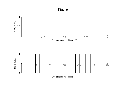
These expressions provide a completely positive map that admit a stochastic interpretation in terms of its associated CTQRW. In Fig. (1) we have implemented a numerical simulation of this quantum stochastic process. We show a set of realizations for the quantum averages of the Pauli matrixes, , . After the first application of the depolarizing superoperator, Eq. (52), the normalized values of and go to zero, remaining in this value at all subsequent times. On the other hand, oscillates between after each scattering event. A notable property of these realizations is the absence of a characteristic time scale both for the first event and for the elapsed time between any successive events. This fact is a consequence of the power law decay of the waiting time distribution , Eq. (44). The absence of any time scale can be seen in the realization of where it is evident the presence of time intervals of any magnitude.
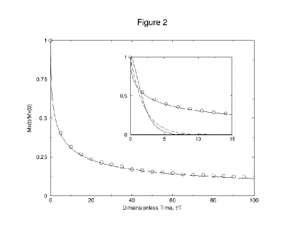
In Fig. (2) we show the corresponding average over realizations together with the analytical result for . We have taken , which allows to use the equivalent expression metzler . In the inset we compare the decay behavior induced by the different kernels. Here, the stretched exponential decay at short times and the power law behavior at long times are evident. In order to be able to compare the different time decay scales induced by each kernel, in all figure of the paper we take , which define the dimensionless time scale .
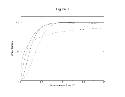
Linear entropy: The linear entropy can be used as a probe of the density matrix positivity. In fact, in a two dimensional Hilbert space, the positivity condition is equivalent to the inequality . This means that if one of the two eigenvalues of is negative, them . Furthermore, the dynamical behaviors induced by each kernel can be shown in a transparent way through this object.
In Fig. (3) we show the linear entropy for the Markovian, exponential and fractional kernels. As initial condition we have chosen a pure state, an eigenstate of . In the case of the exponential kernel, consistently, we verify that independently of the parameter values, the linear entropy is always positive.
III.5.2 Dephasing Reservoir
Here, we assume that the superoperator is defined through the operator
| (72) |
The Lindblad superoperator results in , where
| (73) |
As is well known, this kind of dispersive contribution destroys coherences without affecting the level occupations.
In the case of the exponential kernel, the matrix elements are given by
| (74) |
where the function was defined in Eq. (39) and now . It is simple to proof that independently of any parameter value, here the evolution preserves the density matrix positivity. This follows from the inequality , which, added to the preservation of the probability occupations, guarantees the positivity condition. On the other hand, by expressing the density matrix in the sum representation, , with and , it is immediate to proof that the dynamics is completely positive for any parameter values. Therefore, for this kind of dispersive superoperator, independently of the possibility of associating to it a stochastic dynamics, the solution map is always completely positive.
In the case of the fractional kernel we get
| (75) |
As in the previous environment model, here the coherence decay displays stretched exponential and power law behaviors.
III.5.3 Thermal Reservoir
Now we will analyze a dynamics that leads to a thermal equilibrium state. First, we assume
where and . These operators correspond to a generalized amplitude damping superoperator nielsen . With these definitions, the Lindblad superoperator Eq. (13) can be written as
| (78) |
where was defined in Eq. (73), and
| (79) |
On the other hand, the Lindblad term corresponds to a thermal reservoir
The temperature is defined by , where is the difference of energy between the two levels.
Before proceeding with the description of this case, we want to remark that a pure thermal evolution can be only introduced through an infinitesimal transformation. In fact, it is possible to demonstrate that the superoperator is not a completely positive one, i.e., it can not be written in a sum representation Eq. (3). After noting that the Lindblad superoperator Eq. (78) satisfies , it is possible to associate with the control parameter of Eq. (17). Thus, in the limit the dispersive contribution drops out.
The dynamics induced by the Lindblad Eq. (78) is similar to those analyzed previously in this section. In fact, the solution for the exponential case can be written as in Eqs. (59)-(60) with
| (80) |
On the other hand, for the fractional kernel, the solutions read as in Eqs. (69)-(70) with the definitions
| (81) |
The main difference with the previous solutions are the equilibrium populations which now read , and . As a consequence of this fact, it is simple to realize that for , the exponential kernel produces a mapping that is not completely positive and not even positive. This follows by noting that for , the population solutions Eq. (59) can take negative values.
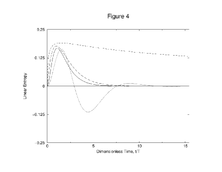
In Fig. (4), for each kernel, we show the linear entropy behavior in the case of a zero temperature reservoir. As in the previous figure, as initial condition we use an eigenstate of the Pauli matrix. In the exponential case, when the stochastic interpretation is not possible the linear entropy takes negative values. Equivalently, this means that is not positive definite.
III.6 Dynamics in a Fock Space
Here we will analyze the dynamics of a CTQRW in a system provided with a Fock space structure, as for example a quantum harmonic oscillator or a mode of an electromagnetic field. With and we denote the corresponding creation and anhilation operators. This situation will allow us to recover the classical concept of continuous time random walks in the context of completely positive maps.
For the superoperator that defines the CTQRW, we assume the following form
| (82) |
where is the displacement operator
| (83) |
Furthermore, we assume that in each application of the complex parameter is chosen with a probability distribution . The induced evolution can be easily analyzed by introducing the Wigner function
| (84) |
whose evolution from Eqs. (14)-(16) then reads
By construction, the solution of this equation provides a completely positive map. Furthermore, we note that this equation can be interpreted as a “classical” continuous time random walk where the statistic of the “particle jumps” is given by and the statistics of the elapsed time between the successive jumps is characterized through the waiting time distribution associated to the kernel . Thus, it is evident that this evolution is a classical one fischer , which implies that any quantum property can only be introduced through the initial conditions.
When all the moments of the distribution are finite, i.e., , , the evolution Eq. (III.6) can be written in terms of a Kramers-Moyal expansion
| (86) |
where the operator is defined by
| (87) |
These expressions follow after developing in Eq. (III.6) the Wigner function around . In this situation, it is also possible to get a close expression for the average excitation number , which reads
| (88) |
Here, we have assumed that the average displacements in the directions are null, i.e., the first moments of the distribution vanish.
Up to second order, the operator reduces to a Hamiltonian term plus a classical Fokker Planck operator. By truncating the evolution up to this order, the CPC is not broken. This fact can be easily demonstrated by going back to the density matrix representation, where the Lindblad superoperator Eq. (16) then reads , with
| (89) |
and
| (90) | |||||
The Lindblad terms proportional to are equivalent to a reservoir at infinite temperature and the terms proportional to and introduce a squeezing effect. On the other hand, it is possible to demonstrate that maintaining only a finite number of higher terms, the evolution for the density matrix can not be written in a Lindblad form and in consequence it is not completely positive. This fact agrees with the predictions of the classical Pawula theorem pawula about Fokker Planck equations.
Subdiffusive Processes: By assuming the fractional kernel Eq. (40), in the limit , , with , the previous second order approximation applies. In this situation, the evolution of the Wigner function is characterized by a subdiffusive process. In fact, the average excitation number reads
| (91) |
Note that in comparison with a Markovian Lindblad evolution, , here the increasing of the average excitations present a slower grow. On the other hand, the evolution of the Wigner function can be written as
| (92) |
Here, is an arbitrary direction in the complex plane, and in order to simplify the expression, we have “traced out” the Wigner function over the perpendicular direction. We remark that this kind of fractional subdiffusive dynamics is allowed in the context of completely positive maps. This equation was extensively analyzed in the literature metzler , where it was found that the solution presents a non-Gaussian diffusion front. We notice that the relations between the exponents that characterize this behavior front were found to be universal in the context of quasiperiodic and disordered systems zhong .
Long Jumps: When the moments of the distribution are not defined, the dynamics must be analyzed in the Fourier domain, . Denoting with a hat symbol the Fourier transform, from Eq. (III.6), we get
where the rates of the Fourier modes is given by
| (93) |
For example, by assuming a Levy distribution metzler , with , the evolution can be written as a series of infinite fractional derivatives with respect to the variables . Nevertheless, with the present formalism, it is not possible to check the CPC of any truncated evolution.
Quantum Random Walks: Finally we note that the concept of quantum random walks julia used in the context of quantum computation and quantum information can be recovered as a particular case of our approach by using the generalized displacement operator
| (94) |
and assuming that , and . Here, is an arbitrary rotation of an extra spin variable, is an arbitrary direction in the complex plane and is the discreet time step.
III.7 Generalized Intrinsic Decoherence Formalism
The intrinsic decoherence formalism milburn ; moya was introduced by Milburn as a phenomenological frame to the description of decoherence phenomema. Here, we will analyze and generalize this formalism by interpreting it as a CTQRW. First, we assume as a superoperator
| (95) |
where is an arbitrary Hamiltonian in a given Hilbert space, and is a random variable chosen with a density probability . From Eqs. (14)-(16), the average density matrix evolves as
In the basis of eigenstates of the Hamiltonian , , the evolution of the matrix elements is given by
| (97) |
Here, the decaying rates read
| (98) |
where , is the Fourier transform of the probability and are the Bohr frequencies.
The original Milburn proposal is obtained by choosing
| (99) |
which implies the density matrix evolution
| (100) |
Thus, our CTQRW provides a natural non-Markovian generalization of this formalism. On the other hand, by choosing the exponential waiting distribution of Eq. (99), , and using the identity , the rate results . This expression coincides with that obtained in the formalism of Ref. bonifaccio .
IV Summary and Conclusions
In this paper we have demonstrated that non-Markovian master equations that consist in a memory integral over a Lindblad structure can be considered as a valid tool in the description of open quantum system dynamics.
Our approach for the understanding of this kind of equations consists in a natural generalization of the classical concept of continuous time random walks to a quantum context. We have defined a CTQRW in terms of a set of random renewal events, each one consisting in the action of a superoperator over a density matrix. The selection of different statistics for the elapsed time between the successive applications of the superoperator allowed us to construct different classes of completely positive evolutions that lead to strong non-exponential decay of the density matrix elements. Remarkable examples are the telegraphic master equation, Eq. (38), which interpolates between a Gaussian short time dynamics and an asymptotic exponential decay, and the fractional master equation, Eq. (41), which leads to stretched exponential and power law behaviors. On the other hand, in a Fock space the dynamics reduces to a classical one, which allowed us to demonstrate that fractional subdiffusive processes are consistent with a completely positive evolution.
Concerning the possibility of obtaining non-physical solutions from the Non-Markovian master equation Eq. (14), we have found a set of mathematical conditions on the kernel that guarantee the CPC of the solution map. As in classical Fokker-Planck equations, the set of conditions Eq. (19) allows us to link each safe kernel with a corresponding waiting time distribution, which in the present case allows to associate to the master equation a CTQRW.
By analyzing the exponential kernel, related to the telegraphic master equation, we have demonstrated that when the kernel can not be associated with a waiting time distribution, the resulting solution map can be either non-physical, only positive, or even completely positive. This case demonstrates that no general conclusions can be obtained outside the regime where a stochastic interpretation is available. Furthermore, we have demonstrated that telegraphic master equations constructed with Lindblad superoperators that can be only introduced through an infinitesimal transformation, Eq. (17), only admit a stochastic interpretation in the Markovian limit. In the case of the fractional kernel we have implemented a numerical simulation that confirms the equivalence between the non-Markovian fractional master equation and the corresponding CTQRW.
Finally we want to remark that from the understating achieved in this work, some interesting open question arise in a natural way, as for example a possible microscopic derivation of these non-Markovian master equations and the finding of alternative stochastic representation based in a continuous measurement theory. In fact, from the examples worked out in this paper, we conclude that the stochastic dynamics of a CTQRW can be thought in a rough way as the continuous measuring action of an environment over an open quantum system, where the scattering superoperator must be associated with the microscopic interaction between the system and the environment, and the statistics of the random times with the spectral properties of the bath.
Acknowledgements.
I am grateful to H. Schomerus and D. Spehner for enlighting discussions.References
- (1) R. Alicki and K. Lendi, in Quantum Dynamical Semigroups and Applications, (Lect. N. in Phys. 286, Springer, 1987).
- (2) M.A. Nielsen and I.L. Chuang, Quantum Computation and Quantum Information, Cambridge University Press (2000).
- (3) V. Wong and M. Gruebele, Chem. Phys. 284, 29 (2002).
- (4) V. Wong and M. Gruebele, Phys. Rev. A 63, 022502 (2001).
- (5) J. Zhong, et. al., Phys. Rev. Lett. 86, 2485 (2001).
- (6) Y. Jung, E. Barkai, and R.J. Silbey, Chem. Phys. 284, 181 (2002).
- (7) V.V. Dobrovitski, et. al., Phys. Rev. Lett. 90, 210401 (2003).
- (8) D. Kuznezov, A. Bulgac, and G.D. Dang, Phys. Rev. Lett. 82, 1136 (1999).
- (9) B.J. Dalton and B.M. Garraway, Phys. Rev. A 68, 033809 (2003).
- (10) W. Feller, An introduction to Probability Theory and Its Applications (J. Wiley & Sons, NY, 1971), Vols. 1 and 2.
- (11) E.W. Montroll and G.H. Weiss, J. Math. Phys. 6, 167 (1965); H. Scher and E.W. Montroll, Phys. Rev. 12, 2455 (1975).
- (12) R. Metzler, and J. Klafter, Phys. Rep. 339, 1 (2000).
- (13) J. Kempe, arXiv: quant-ph/0303081 (2003).
- (14) S.M. Barnett, and S. Stenholm, Phys. Rev. A 64, 033808 (2001).
- (15) I.M. Sokolov, Phys. Rev. E 66, 041101 (2002).
- (16) R. Metzler, E. Barkai, and J. Klafter, Phys. Rev. Lett. 82, 3563 (1999).
-
(17)
In Ref.sokolov the extra conditions
and that must be a CM function are also demanded. By writing the survival probability as
it is simple to realize that these conditions are equivalent to demand the inequality , which implies that this extra conditions are automatically satisfied if the conditions Eq. (19) are satisfied. This follows by noticing that a well defined waiting time distribution always guarantee . - (18) H.J. Briegel, and B.G. Englert, Phys. Rev. A 47, 3311 (1993).
- (19) G. Kimura, Phys. Rev. A 66, 062113 (2002).
- (20) P.M. Morse and H. Feshbach, Methods of Theoretical Physics, Mc Graw Hill Company, (1953).
- (21) Lu-Ming Duan and Guang-Can Guo, Phys. Rev. A 56, 4466 (1997).
- (22) A.A. Budini, Phys. Rev. A 64, 052110 (2001).
- (23) S. Yu, Phys. Rev. A 62, 024302 (2000).
- (24) W. Fischer, H. Leschke, and P. Müller, Phys. Rev. Lett. 73 1578 (1994).
- (25) R.F. Pawula, Phys. Rev. 162, 186 (1967).
- (26) See Eq. (45) in Ref. metzler .
- (27) G.J. Milburn, Phys. Rev. A 44, 5401 (1991).
- (28) H. Moya-Cessa, V. Bužek, M.S. Kim, and P.L. Knight, Phys. Rev. A 48, 3900 (1993).
- (29) R. Bonifacio, et. al., J. Mod. Opt. 47, 2199 (2000); R. Bonifacio, S. Olivares, P. Tombesi, and D. Vitali, Phys. Rev. A 61, 053802 (2000).