Rotating kinky braneworlds

Abstract

Cylindrical braneworlds have been used in the literature as a convenient way to resolve co-dimension-two branes. They are prevented from collapsing by a massless worldvolume field with non-trivial winding, but here we discuss another way of preventing collapse, which is to rotate the brane. We use a simple microscopic field theory model of a domain wall with a condensate for which rotation is a necessity, not just a nice added extra. This is due to a splitting instability, whereby the effective potential trapping the condensate is not strong enough to hold it on the defect in the presence of winding without charge.

We use analytic defect solutions in the field theory (kinky vortons) to construct a thin-wall braneworld model by including gravitational dynamics, and we allow for the rotation required by the microscopic theory. We then discuss the impact rotation has on the bulk and brane geometry, thereby providing an anchor for further cosmological investigations. Our setup naturally leads to worldvolume fields living at slightly different radii, and we speculate on the consequences of this in regard to the fermion mass-hierarchy.

1 Introduction

According to the braneworld idea, all Standard Model matter fields, except for gravity, are confined to a brane that is localized inside a higher dimensional bulk spacetime. This explains why our human experience is limited to only three spatial dimensions, even though additional large (or even infinite) extra dimensions might exist. Since gravity has kinetic support in the bulk, the presence of extra dimensions changes the way sources localized on the brane gravitate. This modified gravitational sector is useful because it provides a phenomenological window to infer the presence of extra dimensions and at the same time it leads to a new perspective on longstanding gravitational puzzles. Importantly, these aspects can be studied by using an effective field theory approach to braneworlds that remains agnostic about the model’s high energy origin. In that context, co-dimension-two braneworlds turned out to be particularly interesting for a variety of reasons:

• The cosmological constant (CC) problem: in 4D gravity the vacuum energy of Standard Model matter fields acts as a cosmological constant and thus destabilizes a Minkowski vacuum (or de Sitter vacuum with phenomenologically small curvature scale) unless some fine-tuning is imposed. This is the essence of the CC problem Zeldovich:1967gd ; Zeldovich:1968zz ; Weinberg1989 ; Burgess:2013ara ; Padilla:2015aaa . Models with two infinite volume extra dimensions offer a built-in mechanism to hide the vacuum energy of Standard Model particles from a brane observer. Rather than producing a 4D de Sitter phase on the brane, vacuum energy deforms the bulk into a cone leaving the brane curvature unaffected. From the perspective of a brane observer, the vacuum energy is therefore decoupled. Unfortunately, it has not yet been possible to exploit this mechanism in a phenomenologically viable way. Specifically, the brane induced gravity model (BIG) Dvali:2000xg ; Kaloper:2007ap , which is based on the DGP mechanism Dvali:2000hr to restore a 4D gravity regime, was found to suffer from ghost instablities in the relevant parameter regime Dubovsky:2002jm ; Hassan:2010ys ; Niedermann:2014bqa ; Eglseer:2015xla . In fact, the authors in Niedermann:2017cel have argued recently that the failure can be understood from a model independent perspective. Their analysis uses a very general spectral decomposition of the gravitational propagator. They have also highlighted a small handful of loopholes to their obstructions, and it remains to be seen whether those can be realized within an extra dimensional context. At the end of this work, we will speculate on this possibility in light of our new results.

• The hierarchy problem: according to the ADD proposal ArkaniHamed:1998rs ; Antoniadis:1998ig models with large (but finite) volume extra dimensions can offer a geometrical explanation for the weakness of gravity, which becomes a consequence of the large extra space volume. Models with two co-dimensions are particularly interesting as they are the most predictive: if the bulk gravitational scale is of order of $\sim\,10\,\mathrm{TeV}$ (or above), a ten mircron (or smaller) sized extra dimension is required in order to realize the observed coupling strength of the gravitational zero mode (unless there are substantial warping effects). This implies both signatures of quantum gravity in collider experiments as well as deviations from the Newtonian inverse square law in table top experiments. The supersymmetric large extra dimensions (SLED) proposal Aghababaie:2003wz (see also Gibbons:2003di ) is a prominent example of such a 6D model and can be understood as the low energy version of a particular supergravity theory.

• Brane cosmology: 6D models provide a minimal playground to study cosmological signatures of the braneworld paradigm. Note that this program has been realised in five dimensions in the case of the Randall-Sundrum model Randall:1999ee ; Randall:1999vf (see also Maartens:2010ar for a review on brane cosmology) but little work has been done in higher dimensions due to a simple physical reason: in general, a brane with more than one co-dimension acts as an antenna of gravitational waves if the brane undergoes cosmological evolution Niedermann:2014yka ; Niedermann:2014bqa . This in turn makes it difficult to describe the full time-dependent, coupled system of bulk-brane equations consistently. However, it is this type of new dynamical feature that might also lead to a rich phenomenology, both for finite and infinite volume models.

Despite their phenomenological prospects, co-dimension-two braneworlds suffer from a technical difficulty which is absent in one co-dimension: spacetime curvature diverges at the position of an infinitely thin co-dimension-two brane. This can be understood as the gravitational analogue of a charged string in electrodynamics for which the Coulomb field diverges logarithmically. In the case of a pure tension brane this is a rather mild conical singularity, which can be modelled in terms of a two-dimensional delta-function. However, this is no longer possible for cosmological brane matter with FLRW symmetries Vinet:2004bk . This problem is typically dealt with by blowing up the transverse brane directions. A particularly popular choice consists in replacing the string-like brane by a hollow cylinder (or ring from a purely extra dimensional perspective). This is convenient because then the brane becomes locally a co-dimension-one object, making Israel’s covariant matching techniques Israel:1966rt applicable. This type of brane model was first introduced in Peloso:2006cq to regularize a flux-stabilized, compact (rugby ball shaped) 6D model but later also applied to models with infinite volume extra dimensions Kaloper:2007ap ; Eglseer:2015xla . In a more generic context, it was used in Burgess:2008yx to derive (renormalized) matching conditions of co-dimensions-two braneworlds. In order to prevent the brane’s compact direction from collapsing, a massless scalar field is added to its worldvolume theory. The scalar winds around the brane, thereby providing the angular pressure needed to stabilize the cylinder’s radial direction. Building up on these result, later work often used an angular pressure component of the brane energy-momentum tensor to effectively implement this stabilisation mechanism, rather than resolving it in terms of a worldvolume scalar field (see for example Niedermann:2014bqa ; Niedermann:2014vaa ; Niedermann:2015vbk ).

This work is guided by the question as to whether it is possible to consistently embed the hollow cylinder construction in a (classical) mircrophysical theory that resolves the brane at high energies. In order to maintain a high level of generality, we study this setup within a minimal extra dimensional framework, which should make it possible to extent our construction to established finite (e.g. the rugby ball models Peloso:2006cq ; Aghababaie:2003wz ; Niedermann:2015vbk ) and infinite (e.g. the BIG model Kaloper:2007ap ) volume braneworld models, or to further study it in its minimal form in accordance with the inflating “cigar” proposal in Niedermann:2014yka . Specifically, we will use a domain wall solution that is bent into a cylinder in order to model the brane sector. A cylindrical collapse can then be avoided by localizing a condensate inside the wall (or brane equivalently). These configurations are known as kinky vortons Battye:2008zh ; Battye2009a ; Battye:2009nf and were studied in two spatial dimensions as a proxy for closed loops of superconducting cosmic strings in three dimensions (so-called vortons Davis:1988jq ). Due to the trapping of the condensate the brane carries winding and charge, which both contribute towards its stability. In fact, for kinky vortons it is known Battye:2008zh that the charge is a vital ingredient to avoid non-axial instabilities, whereby the potential trapping the condensate is not strong enough to hold on to it.

The important realization of Sec. 2 is that the condensate’s Nöther charge leaves a low energy fingerprint in the form of a non-vanishing angular momentum of the brane, and hence cannot be characterized by an angular pressure (or winding) alone. Correspondingly, the requirement of having a consistent microphysical description in terms of a kinky vorton forces us to include angular momentum in our low energy description. This is an important observation for two reasons: Firstly, it introduces rotation as a new dynamical feature of 6D braneworlds which to our knowledge has not been considered before, and secondly, it raises the question as to whether alternative ultraviolet (UV) embeddings might lead to the same conclusion, making it hence imperative to include rotation to the low energy description.

While answering this UV-sensitive question goes beyond the scope of the present work, we devote Sec. 3 to a first discussion of the implications rotation has on the spacetime geometry. This is done within a thin-wall approximation that makes explicit contact with the established models based on a worldvolume description of the brane. We are able to derive explicit solutions of the coupled gravitational system, including the bulk Einstein and brane matching equations. We then find two types of solutions; those for which the bulk geometry asymptotes to a cone (sub-critical) and those for which the bulk closes in a second axis (super-critical). These solutions can serve as an anchor for more detailed cosmological investigations of both finite and infinite volume scenarios. In particular, in the non-rotating limit the super-critical branch of our braneworld model has recently been shown to feature a new mechanism to realize an inflationary phase on the brane Niedermann:2014yka and thus holds greater phenomenological promise.

We will conclude our work in Sec. 4 by discussing different directions of future research, and possible implications for the fermion mass hieracrchy.

2 Kinky vortons

The idea behind a kinky vorton is to construct a domain wall (kink) in two spatial dimensions, and then bend it into a circle. This, however, would be unstable, as the tension in the kink would cause the radius of the ring to reduce, and the kink would eventually collapse and decay into radiation. To prevent this from happening we may put a condensate on the kink, and arrange it such that the condensate stabilizes the vorton at some radius, with the condensate providing both Nöther charge and winding number to contribute towards stability. We now discuss such a model, as described in Battye:2008zh ; Battye:2009nf .

2.1 Microphysical description

The field responsible for the domain wall is taken to be a real scalar field $\Phi$ with the standard symmetry-breaking potential, and we take the condensate field to be a complex scalar $\Sigma$, again with the standard symmetry-breaking form. The two fields have a bi-quadratic coupling leaving us with

$${\cal L} = -\frac{1}{2}\,\partial_{\mu}\Phi\partial^{\mu}\Phi-\partial_{\mu}\Sigma^{\dagger}\partial^{\mu}\Sigma-\frac{1}{4}\,\lambda_{\Phi}\,\left(\Phi^{2}-\eta_{\Phi}^{2}\right)^{2}-\frac{1}{4}\,\lambda_{\Sigma}\left(|\Sigma|^{2}-\eta_{\Sigma}^{2}\right)^{2}-\beta\,\Phi^{2}\,|\Sigma|^{2}+\frac{1}{4}\,\lambda_{\Sigma}\,\eta^{4}_{\Sigma}.$$

We shall take our model to live in $d$ spacetime dimensions, and label the co-ordinates such that the fields are independent of $z$, with $x$ being the transverse co-ordinate, and the current being in the $y$-direction. Later, when we come to the circular vorton, then the radial co-ordinate $r$ will play the role of $x$, and the azimuthal direction $\phi$, along which the current flows, will play the role of $y$, and we shall keep the notation $z$ for those directions along which the fields do not depend (see Fig. 1).

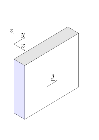
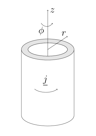
Figure 1: A sketch of the orientation of the domain wall and the vorton, each with current $\underline{j}$.

The constant term in the Lagrangian density is to ensure that $V(\Phi=\pm\eta_{\Phi},\;\Sigma=0)=0$. The condensate is taken to be of the form

$$\Sigma = |\Sigma|(x)\exp\{i\sigma(t,y)\}=|\Sigma|(x)\exp\{i[\omega t+ky]\},$$ (2)

and we define the quantity $\chi$, which is used to characterize vortons as electric ($\chi>0$), chiral ($\chi=0$) or magnetic ($\chi<0$),

$$\chi = \omega^{2}-k^{2}.$$ (3)

The magnitude of the condensate field, $|\Sigma|$, is to vanish away from the kink, and take some non-zero value on the kink. In order to achieve this we note that the effective potential for the condensate in the core of the kink ($\Phi=0$) is given by

$$V(\Phi=0,\Sigma) = \frac{1}{4}\lambda_{\Sigma}\left(|\Sigma|^{2}-\eta^{2}_{\Sigma}-\frac{2\chi}{\lambda_{\Sigma}}\right)^{2}+C,$$ (4)

$$C = -\frac{1}{4}\lambda_{\Sigma}(\eta^{2}_{\Sigma}+2\chi/\lambda_{\Sigma})^{2}+\frac{1}{4}\lambda_{\Phi}\eta^{4}_{\Phi}$$ (5)

and so for a non-zero $\Sigma$-condensate to form, we require

$$\eta_{\Sigma}^{2}+\frac{2\chi}{\lambda_{\Sigma}}>0,$$ (6)

and then the condensate has value $|\Sigma|^{2}=\eta_{\Sigma}^{2}+\frac{2\chi}{\lambda_{\Sigma}}$, which minimizes $V$.

In order to ensure the spontaneous breaking of the $\mathbb{Z}_{2}$ symmetry $\Phi\to-\Phi$, and hence the formation of a kink, we impose that the global vacua are $(\Phi=\pm\eta_{\Phi},\;\Sigma=0)$, and so require the condensate on the kink to have an energy penalty compared to the global vacuum, $V(\Phi=0,\;|\Sigma|^{2}=\eta_{\Sigma}^{2}+\frac{2\chi}{\lambda_{\Sigma}})>V(\Phi=\pm\eta_{\Phi},\;\Sigma=0)$ . This leads to

$$\eta^{4}_{\Phi}\frac{\lambda_{\Phi}}{\lambda_{\Sigma}}>\left(\eta_{\Sigma}^{2}+2\chi/\lambda_{\Sigma}\right)^{2}.$$ (7)

Finally, we wish to ensure that no condensate forms when $\Phi=\pm\eta_{\Phi}$, and so we note that a positive quadratic term in

$$V(\Phi=\pm\eta_{\Phi},\;\Sigma) = \left(\beta\eta^{2}_{\Phi}-\frac{1}{2}\lambda_{\Sigma}\eta^{2}_{\Sigma}-\chi\right)|\Sigma|^{2}+\frac{1}{4}\lambda_{\Sigma}|\Sigma|^{4}+constant$$ (8)

would prevent such a breaking of the U(1) symmetry by the presence of a condensate, which necessitates

$$\beta>\frac{\lambda_{\Sigma}}{2}\frac{\eta^{2}_{\Sigma}+2\chi/\lambda_{\Sigma}}{\eta^{2}_{\Phi}}.$$ (9)

At this point we make a parameter choice that will allow us to find analytic solutions, by imposing that (7) and (9) are equivalent. This leads to

$$\beta=\frac{1}{2}\sqrt{\lambda_{\Phi}\lambda_{\Sigma}}.$$ (10)

The analytic solution in question is

$$\Phi = \eta_{\Phi}\tanh(ax),$$ (11a)

$$|\Sigma| = \frac{b}{\cosh(ax)},$$ (11b)

$$a^{2} = \beta\eta_{\Phi}^{2}-(\chi+\lambda_{\Sigma}\eta_{\Sigma}^{2}/2),$$ (11c)

$$b^{2} = \frac{2}{\lambda_{\Sigma}}(2(\chi+\lambda_{\Sigma}\eta_{\Sigma}^{2}/2)-\beta\eta_{\Phi}^{2}),$$ (11d)

which further requires

$$\lambda_{\Sigma} = 4\beta,$$ (12)

and then (10) gives $\lambda_{\Phi}=\beta$. Having found the analytic solution for a kink with a condensate, we need to ensure that the solution parameters $a$ and $b$ are real, leading to

$$2\beta\eta_{\Sigma}^{2}+\chi<\beta\eta_{\Phi}^{2}<2(2\beta\eta_{\Sigma}^{2}+\chi).$$ (13)

At this point we make another choice of parameters, which ensures a symmetric range in possible values of $\chi$

$$\eta_{\Phi}^{2} = \frac{8}{3}\eta_{\Sigma}^{2},$$ (14)

leading to

$$-1<4\tilde{\chi}<1,$$ (15)

where we have introduced the dimensionless quantity

$$\tilde{\chi} = \frac{\chi}{\beta\eta_{\Phi}^{2}}.$$ (16)

We also note that the scale for the thickness of the domain wall is given by

$$({\rm thickness})^{-1}=a=\frac{1}{2}\,\sqrt{\beta\eta_{\Phi}^{2}}\,\sqrt{1-4\tilde{\chi}},$$ (17)

and from now on we work in units where $\beta\eta_{\Phi}^{2}=1$. We are now in a position to evaluate some physical properties of the straight kink-vorton, so we start by defining the Nöther current, $j_{\mu}$, and charge, $Q$,

$$j_{\mu} = -\frac{i}{2}\,\left(\Sigma^{\dagger}\partial_{\mu}\Sigma-\partial_{\mu}\Sigma^{\dagger}\Sigma\right),$$ (18)

$$Q/V_{z} = \int\,\mathrm{d}x\,\mathrm{d}y\,j_{0}=\omega\,\int\mathrm{d}x\,\mathrm{d}y\,|\Sigma|^{2},$$ (19)

where $V_{z}$ is the volume in the $\underline{z}$ directions.

The Hamiltonian for (LABEL:eq:fieldTheoryFullLagrangian) is calculated in the standard way, and its spatial integral gives the energy. Taking the analytic solution, and the specified choices of parameters, allows us to derive the energy and charge of the straight domain wall as

$$E/(L_{y}\,V_{z}) = {\cal E}/L_{y}=\frac{8\,\chi^{2}-10\,\chi+5+6\,(1+4\,\chi)(k^{2}+\omega^{2})}{6\,\beta\sqrt{1-4\,\chi}},$$ (20)

$$Q/(L_{y}\,V_{z}) = {\cal Q}/L_{y}=\frac{\omega\,(1+4\,\chi)}{\beta\,\sqrt{1-4\,\chi}},$$ (21)

where $L_{y}$ is the length of the domain wall in the $y$ direction.

Having found the exact form of the straight kinky vortons, we now look to what happens when we bend them into a circle. The idea is that while a condensate-free kink is bound to collapse under its own tension, the presence of a condensate may stabilize the collapse. The belief was that a closed loop with a condensate of definite winding number

$$N = \frac{2\pi}{\lambda}R=kR,$$ (22)

without charge, would be enough to prevent collapse Ostriker:1986xc ; Copeland:1987th ; Haws:1988ax ; Copeland:1987yv , but a more complete analysis revealed that in fact the angular momentum of the loop, when charge is also present, was the important factor Davis:1988jq ; Davis:1988ip ; Davis:1988ij . Even when both charge and winding number are present, one must be careful about making statements of stability, as circular vortons may be unstable against non-circular perturbations, in particular there may be pinch instabilities Battye:2008zh .

For this analysis we follow Battye:2008zh and consider the approximate solution of a large radius vorton composed with the field profiles of the analytic solution. Taking the square of (21) for a vorton of radius $R$ ($L_{y}=2\pi R$), and using $\omega^{2}=\chi+k^{2}$ we find that

$$16\chi^{3}+8\left(1+\frac{2N^{2}}{R^{2}}\right)\chi^{2}+\left(1+\frac{8N^{2}}{R^{2}}+\frac{4\beta^{2}{\cal Q}^{2}}{4\pi^{2}R^{2}}\right)\chi+\left(N^{2}-\frac{\beta^{2}{\cal Q}^{2}}{4\pi^{2}}\right)\frac{1}{R^{2}} = 0\,.$$ (23)

In order to get a feel for how $R$ varies with $\chi$ according to this equation we show some examples in Fig. 2 for fixed winding number and charge.

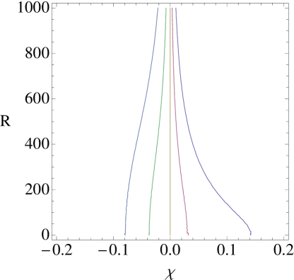
Figure 2: A plot showing how $R$ varies with $\chi$, for $N=200$ (left), $150$, $\frac{\beta{\cal Q}}{2\pi}$, $100$, and $50$ (right) in the case $2\beta{\cal Q}=1500$, in units where $\beta\eta_{\Phi}^{2}=1$.

We will be interested in the thin-wall limit, $R>>1$, which takes us to $\chi\sim 0$, as can be seen from Fig. 2. In fact, (23) gives a thin-wall approximation to $\chi$ of

$$\chi_{tw} \simeq \frac{\left(\frac{\beta{\cal Q}}{2\pi}\right)^{2}-N^{2}}{1+\frac{4\left(\frac{\beta{\cal Q}}{2\pi}\right)^{2}+8N^{2}}{R^{2}}}\frac{1}{R^{2}}.$$ (24)

We now wish to find the energy-minimizing radius, so proceed to calculate the energy by taking (21) and (20), which leads to

$${\cal E} = \frac{2\pi}{\beta\sqrt{1-4\chi}}\left[\frac{R}{3}\left(4\chi^{2}-5\chi+\frac{5}{2}\right)+\frac{1}{R}\left(N^{2}(1+4\chi)+\left(\frac{\beta{\cal Q}}{2\pi}\right)^{2}\frac{1-4\chi}{1+4\chi}\right)\right].$$ (25)

We now minimize this with respect to $R$, taking $\chi$ to be effectively independent of $R$ in the thin-wall limit, to find the minimum-energy vorton radius to be

$$R_{0}^{2} = 3\frac{(1+4\chi)N^{2}+\frac{1-4\chi}{1+4\chi}\left(\frac{\beta{\cal Q}}{2\pi}\right)^{2}}{4\chi^{2}-5\chi+5/2}.$$ (26)

The final quantity of interest is the angular momentum of the vorton, established in Minkowski spacetime as

$$J = \int\mathrm{d}\phi\,\mathrm{d}r\,\mathrm{d}z\,r\,T^{t}_{\;\phi}$$ (27)

$$= 2\pi V_{z}\int\mathrm{d}r\,r\,2\,\omega\,k\,|\Sigma|^{2}$$

$$= 2\,k\,{\cal Q}\,V_{z}.$$

So we introduce the angular momentum per unit $z$-volume ${\cal J}=J/V_{z}$, to find

$${\cal J} = 2\frac{N{\cal Q}}{R}.$$ (28)

We are now in a position to be able to calculate the energy-minimizing radius $R$ and quantity $\chi$ by specifying the winding number $N$ and the charge ${\cal Q}$. This follows by substituting $R_{0}$ from (26) into (23) and solving, numerically, for $\chi$. This $\chi$ is then used in (26) to find the radius $R_{0}$. As this analysis for circular vortons uses the analytic solution for straight kinks, then we only expect this approximation to hold for large radii. For example, Battye:2008zh have shown that for winding numbers greater than 10 and radii greater than 50 the approximation and full field theory simulations are in agreement. Importantly, they also found no solutions for a number of cases, such as ${\cal Q}=500$ (or $N=10$). This highlights that the microphysics plays an important role in the existence of these large-scale defects, and so to construct a consistent braneworld model one must take this physics into account. In particular, it was seen in Battye:2008zh that if ${\cal Q}=0$ (or $N=0$), then the vortons have zero radius which, in the context of braneworlds constructed with these domain walls, would rule out braneworlds that are “stabilized” by winding alone.

2.2 Thin wall description

We may now take the analytic solution for the vortons and come up with an effective action in the thin-brane limit by integrating the field theory action transverse to the kink,

$$S = \int{\rm d}x\int{\rm d}t\,{\rm d}y\,{\cal L},$$ (29)

where by imposing the ansatz (11a-11b) along with $\Sigma=|\Sigma|\exp\{i\sigma(t,y)\}$ we may perform the $x$-integration to yield

$$S = \int{\rm d}t\,{\rm d}y\,\left[-\frac{1}{2}\,\partial_{\mu}\tilde{\sigma}\partial^{\mu}\tilde{\sigma}-\lambda_{(d-1)}\right],$$ (30a)

$$\tilde{\sigma}^{2} = \frac{2\,(1+4\,\chi)}{\beta\,\sqrt{1-4\,\chi}}\sigma^{2},$$ (30b)

$$\lambda_{(d-1)} = \frac{8\,\chi^{2}-10\,\chi+5}{6\,\beta\sqrt{1-4\,\chi}},$$ (30c)

so the kinky-wall looks like a thin wall with a canonical massless scalar, $\tilde{\sigma}$, living on it.

The energy of a kink with a condensate is found by calculating the Hamiltonian from the action, and yields

$${\cal E} = 2\pi R\,\lambda_{3}+\frac{\pi\,\tilde{N}^{2}}{R}+\pi R\,\tilde{\omega}^{2},$$ (31)

where we have introduced the rescaled $\omega$ and $N$

$$\tilde{\omega}^{2} = \frac{2\,(1+4\,\chi)}{\beta\,\sqrt{1-4\,\chi}}\,\omega^{2},\qquad\tilde{N}^{2}=\frac{2\,(1+4\,\chi)}{\beta\,\sqrt{1-4\,\chi}}\,N^{2},$$ (32)

and find that the expression for energy matches the previous expression (20), as it should. In the next section we will use the thin wall description to study the gravitational response within a six dimensional braneworld model.

3 Kinky braneworlds

Here we employ the kinky vorton as a microscopic core model for a 4-brane, $\Sigma_{4}=\mathbb{R}^{3}\times\mathcal{S}^{1}$, with three infinite and one circular spatial dimension. In other words, we consider the case for which the axial direction corresponds to a three dimensional manifold [with coordinates $\underline{z}=(z_{1},z_{2},z_{3})$] describing the spatial dimensions of our universe. Accordingly, the circular vorton dimension plays the role of a compact brane dimension, see Fig. 1.

We are mainly interested in the gravitational response of the coupled vorton-gravity system. As this is hard to solve analytically, we employ the effective theory introduced via (30a) to describe the system in the thin brane limit. Correspondingly, the worldvolume theory in its covariant form reads

$$S_{\mathrm{brane}}=\int\mathrm{d}^{5}\tilde{x}\,\sqrt{-\det\left(\tilde{g}\right)}\left[-\frac{1}{2}\partial_{\tilde{\mu}}\tilde{\sigma}\partial^{\tilde{\mu}}\tilde{\sigma}-\lambda_{5}+M_{6}^{4}\Delta K\right]\;,$$ (33)

where the last term is the Gibbons-Hawking-York boundary term, constructed out of the extrinsic curvature $K$.

3.1 Bulk-brane system

We start with the exterior, $r>R_{0}$, bulk metric,

$$\mathrm{d}s^{2}_{\mathrm{ext}}=-\,u(r)\,\left[\mathrm{d}t+a(r)\,\mathrm{d}\varphi\right]^{2}+\mathrm{e}^{2\,k(r)/3}\mathrm{d}\underline{z}^{2}+F^{2}\,\mathrm{e}^{2\,k(r)}\mathrm{d}r^{2}+r^{2}\,u(r)^{-1}\mathrm{d}\varphi^{2}\;,$$ (34)

which adapts the ansatz used by Davies (and first introduced in levy_robinson_1964 ) to describe a rotating cylinder to 6D. The constant $F$ accounts for the presence of a conical deficit angle. The corresponding vacuum field equations read

$$2\,F^{2}\,\frac{\mathrm{e}^{2k}}{u}\,R_{tt} \equiv\frac{1}{\,r^{2}}\left(u\,a^{\prime}\right)^{2}-\left(\frac{u^{\prime}}{u}\right)^{2}+\frac{1}{r}\,\frac{u^{\prime}}{u}+\frac{u^{\prime\prime}}{u}=0\;,$$ (35a)

$$F^{2}\,\mathrm{e}^{2\left(k-u\right)}\,\left(R_{t\varphi}-aR_{tt}\right) \equiv a^{\prime\prime}-\frac{1}{r}\,a^{\prime}+2\,a^{\prime}\,\frac{u^{\prime}}{u}=0\;,$$ (35b)

$$R_{rr}-3\,F^{2}\,\mathrm{e}^{4k/3}R_{zz} \equiv\frac{1}{2\,r^{2}}\,\left(u\,a^{\prime}\right)^{2}+\frac{1}{r}\,\left(2\,k^{\prime}+\frac{u^{\prime}}{u}\right)+\frac{2}{3}\left(k^{\prime 2}-\frac{3}{4}\,\left(\frac{u^{\prime}}{u}\right)^{2}\right)=0\;.$$ (35c)

The first two equations coincide with the 4D ones, and they are solved by

$$u(r) =\frac{1-B\left(|E|\,r\right)^{2\,A}}{A\sqrt{|B|}\left(|E|\,r\right)^{A-1}}\;,$$ (36a)

$$a(r) =-\,\frac{A}{E\left[1-B\,(|E|\,r)^{2A}\right]}+C\;,$$ (36b)

where $A$, $B$, $C$ and $E$ are integration constants. Eq. (35c) then implies

$$4\,r\,k^{\prime}\left(3+r\,k^{\prime}\right)=3\,\left(A^{2}-1\right)\;,$$ (37)

which is different from its 4D counterpart and solved by

$$k_{\pm}(r)=\frac{1}{2}\left(-3\pm\,\sqrt{3}\sqrt{2+A^{2}}\right)\log\left(D\,r\right)\;,$$ (38)

where $D$ is a constant. Only the branch $k=k_{+}$ is continuously connected to the trivial solution $k=0$. Later we will see that this branch has to be chosen in order to describe the geometry of a thin vorton configuration.

The spacetime region inside the brane uses radial coordinate $\bar{r}$, and is assumed to be Minkowskian (in accordance with the findings in Davies ), which in a non-rotating frame reads

$$\mathrm{d}s^{2}_{\mathrm{int}}=-\mathrm{d}t^{2}+\mathrm{d}\underline{z}^{2}+\mathrm{d}\bar{r}^{2}+\bar{r}^{2}\mathrm{d}\varphi^{2}\;.$$ (39)

Further, by introducing the brane coordinates $\tilde{x}^{\tilde{\alpha}}=(t,\underline{z},\varphi)$, we can parametrise the brane induced metric as

$$\mathrm{d}\tilde{s}^{2}=-\mathrm{d}t^{2}+\mathrm{d}\underline{z}^{2}+R_{0}^{2}\,\mathrm{d}\varphi^{2}\;.$$ (40)

Continuity of the metric across the brane then requires

$$a|_{r=R_{0}}=0\,, u|_{r=R_{0}}=1\,, k|_{r=R_{0}}=0\,.$$ (41)

which in turn implies

$$D =1/R_{0}\;,$$ (42a)

$$B =\frac{1}{4}\,(R_{0}\,|E|)^{-2\left(A+1\right)}\left[A-\sqrt{A^{2}+4\,R_{0}^{2}\,E^{2}}\right]^{2}\;,$$ (42b)

$$C =\frac{A}{E\left[1-B\left(R_{0}|E|\right)^{2A}\right]}\;.$$ (42c)

The remaining integration constants are fixed in terms of the brane matter through Israel’s junction conditions,

$$\Delta K^{\tilde{\mu}}_{\;\tilde{\nu}}\,-\,\delta^{\tilde{\mu}}_{\tilde{\nu}}\,\Delta K\,= \,\frac{1}{M_{6}^{4}}\left[T^{\tilde{\mu}}_{(\tilde{\sigma})\tilde{\nu}}-\lambda_{5}\,\delta^{\tilde{\mu}}_{\tilde{\nu}}\right]\;.$$ (43)

Here we may think of the tension $\lambda_{5}$ combining with the matter stress-tensor to provide the total brane stress-tensor $T_{(brane,tot)}^{\tilde{\mu}\tilde{\nu}}=T_{(\tilde{\sigma})}^{\tilde{\mu}\tilde{\nu}}\,-\,\lambda_{5}\,\tilde{g}^{\tilde{\mu}\tilde{\nu}}$. We also introduced the discontinutiy of the extrinsic curvature across the brane,

$$\Delta K^{\tilde{\mu}}_{\;\tilde{\nu}}:=K^{\tilde{\mu}}_{\mathrm{(int)}\tilde{\nu}}\Big{|}_{\bar{r}=R_{0}}+K^{\tilde{\mu}}_{\mathrm{(ext)}\tilde{\nu}}\Big{|}_{r=R_{0}}\;.$$ (44)

We used the convention where the interior normal vector points outwards and the exterior normal vector points inwards, explicitly $n_{\mathrm{int}}=\partial_{\bar{r}}$ and $n_{\mathrm{ext}}=-K\,\mathrm{e}^{k(r)}\partial_{r}$. Then the Minkowskian geometry in the interior implies $K^{\varphi}_{\mathrm{(int)}\varphi}=1/R_{0}$ as the only non-vanishing component. On the other hand, the exterior geometry (34) has the following non-zero extrinsic curvature components (evaluated at the brane)

$$K_{(\mathrm{ext})t}^{t} =-\,\frac{1}{2\,F}\,u^{\prime}|_{r=R_{0}}=\frac{-1+\sqrt{A^{2}+4\,R_{0}^{2}\,E^{2}}}{2\,F\,R_{0}}\;,$$ (45a)

$$K_{(\mathrm{ext})\varphi}^{t} =-\,\frac{1}{2\,F}\,a^{\prime}|_{r=R_{0}}=\frac{R_{0}\,E}{F}\;,$$ (45b)

$$K_{(\mathrm{ext})\varphi}^{\varphi} =-\,\frac{1}{2\,F\,R_{0}}\,\left[2-R_{0}\,u^{\prime}\right]_{r=R_{0}}=\frac{-1-\sqrt{A^{2}+4\,R_{0}^{2}\,E^{2}}}{2\,F\,R_{0}}\;,$$ (45c)

$$K_{(\mathrm{ext})t}^{\varphi} =-\frac{E}{F\,R_{0}}\;,$$ (45d)

$$K_{(\mathrm{ext})1}^{1} =-\,\frac{1}{3\,F}\,k^{\prime}|_{r=R_{0}}=\frac{3\mp\sqrt{3}\,\sqrt{2+A^{2}}}{6\,F\,R_{0}}\;,$$ (45e)

where the upper sign corresponds to the choice $k=k_{+}$ and the lower one to $k=k_{-}$. The matter field is taken to have the following form

$$\tilde{\sigma}=\mu_{0}^{3/2}\left(\omega\,t+N\varphi\right)\equiv\tilde{\omega}\,t+\tilde{N}\,\varphi\;,$$ (46)

where $N$ is the winding number introduced before and $\mu_{0}$ a mass scale, which, according to (30b), is fixed by the underlying vorton model,

$$\mu_{0}^{3}=\frac{2\,\left(1+4\,\chi\right)}{\beta\sqrt{1-4\,\chi}}\;.$$ (47)

The brane-induced stress tensor has the following non-zero components,

$$T^{t}_{(\sigma)\;t} =-\frac{\mu_{0}^{3}}{2}\left(\omega^{2}+\frac{N^{2}}{R_{0}^{2}}\right)\;, T^{t}_{(\sigma)\;\varphi} =\mu_{0}^{3}\,\omega N\;,$$ (48a)

$$T^{\varphi}_{(\sigma)\;\varphi} =\frac{\mu^{3}_{0}}{2}\left(\omega^{2}+\frac{N^{2}}{R_{0}^{2}}\right)\;, T^{\varphi}_{(\sigma)\;t} =-\frac{\mu_{0}^{3}}{R_{0}^{2}}\,\omega\,N\;,$$ (48b)

$$T^{z}_{(\sigma)\;z} =\frac{\mu_{0}^{3}}{2}\left(\omega^{2}-\frac{N^{2}}{R_{0}^{2}}\right)\;.$$ (48c)

It is further convenient to introduce the dimensionless quantities

$$\bar{\lambda}=\frac{2\,R_{0}\,\lambda_{5}}{M_{6}^{4}}\;, \bar{\omega}^{2}=\frac{R_{0}\,\mu_{0}^{3}\,\omega^{2}}{M_{6}^{4}}\;, \bar{q}^{2}=\frac{\mu_{0}^{3}\,N^{2}}{R_{0}\,M_{6}^{4}}\;,$$ (49)

where $M_{6}$ is the gravitational scale in the bulk. We are now ready to evaluate the junction conditions (43), yielding four independent equations,

$$\left(t\atop\varphi\right): \frac{E\,R_{0}}{F} =\bar{q}\,\bar{\omega}\;,$$ (50a)

$$6\,\left(z\atop z\right)-2\,\left(t\atop t\right)-2\,\left(\varphi\atop\varphi\right): \frac{4}{F} =4+3\,\left(\bar{\omega}^{2}-\bar{q}^{2}\right)-\bar{\lambda}\;,$$ (50b)

$$\left(t\atop t\right)-\left(\varphi\atop\varphi\right): \frac{\sqrt{A^{2}+4\,R_{0}^{2}\,E^{2}}}{F} =\left(1-\bar{q}^{2}-\bar{\omega}^{2}\right)\;,$$ (50c)

$$\left(z\atop z\right): \frac{2\,\sqrt{3}\,\sqrt{2+A^{2}}}{F} =\pm\,3\left(2+\bar{\omega}^{2}-\bar{q}^{2}-\bar{\lambda}\right)\;,$$ (50d)

where the “+” and “–” sign in the last equation correspond to $k=k_{+}$ and $k=k_{-}$, respectively. We obtain

$$F =\frac{E\,R_{0}}{\bar{q}\,\bar{\omega}}\;,$$ (51a)

$$R_{0}\,E =\frac{4\,\bar{q}\,\bar{\omega}}{4-3\,\bar{q}^{2}-\bar{\lambda}+3\,\bar{\omega}^{2}}\;,$$ (51b)

$$A^{2} =16\,\frac{\bar{q}^{4}+\left(1-\bar{\omega}^{2}\right)^{2}-2\,\bar{q}^{2}\left(1+\bar{\omega}^{2}\right)}{\left[4-3\,\bar{q}^{2}-\bar{\lambda}+3\,\bar{\omega}^{2}\right]^{2}}\;,$$ (51c)

where $\bar{\omega}$ and $\bar{\lambda}$ have to be chosen such that $A$ is real.

Since all geometry related integration constants have been fixed, the remaining equation in (50d) provides a constraint on the brane parameters as specified in (49). In particular, it determines the radius $R_{0}$ once the winding number $N$, tension $\lambda_{5}$ and frequency $\omega$ have been fixed. After using the expressions in (51), the constraint (50d) reads

$$\pm\sigma_{1}\,\sqrt{17\,\bar{q}^{4}-\left(8-\bar{\lambda}\right)\bar{\lambda}-6\,\bar{\lambda}\,\bar{\omega}^{2}+17\,\bar{\omega}^{4}-\bar{q}^{2}\left(40-6\bar{\lambda}+34\,\bar{\omega}^{2}\right)+8\left(3+\bar{\omega}^{2}\right)}\\ -\sqrt{6}\,\left(2+\bar{\omega}^{2}-\bar{\lambda}-\bar{q}^{2}\right)=0\;,$$ (52)

where $\sigma_{1}=\mathrm{sgn}\left(4+3\,\bar{\omega}^{2}-3\,\bar{q}^{2}-\bar{\lambda}\right)$. Again, the “+” and “–” sign corresponds to $k=k_{+}$ and $k=k_{-}$, respectively.

3.2 Parameter space

As a first sanity check, we try to make contact with the Minkowski analysis. To that end, we take the decoupling limit ($M_{6}\to\infty$) of the above equation, corresponding to $\left\{\bar{q}^{2},\,\bar{\omega}^{2},\,\bar{\lambda}\right\}\ll 1$. This implies $\sigma_{1}=1$ and requires the “+” sign in (52). Later, we will see that this choice leads to a conical geometry if we depart from the decoupling limit. At first non-vanishing order, we find

$$\bar{q}^{2}+\bar{\omega}^{2}-\bar{\lambda}\approx 0\;,$$ (53)

which after restoring $R_{0}$, using (49), becomes

$$\frac{N^{2}}{R^{2}_{0}}+\omega^{2}-2\,\mu_{0}^{-3}\lambda_{5}\approx 0\;.$$ (54)

By using the definitions in (21), (30c) and (47), we can show that this is identical to the expression in (26), constituting a nice consistency check of our calculations. Note that the above equation also admits solutions for $\omega=0$ which correspond to $R_{0}>0$. These solutions are not supported by our kinky vorton model which implies a collapse in this case. The mismatch occurs because the thin-wall approximation in (24), which we used to derive the EFT, breaks down in that particular case. We still include this case in our discussion here, because it allows us to make contact with well-studied conical geometries in the literature.

In the next step, we go away from the decoupling limit and discuss the solutions of (52) in greater generality.

Conical branch

Here we pick the “+” sign in (52), corresponding to $k=k_{+}$ in (38). This branch is of particular interest as it admits a consistent decoupling limit. We find two solutions

$$\bar{q}^{2}_{\pm}=\frac{1}{11}\,\left[8+3\,\bar{\lambda}+11\,\bar{\omega}^{2}\pm 4\,\sqrt{4\left(1-\bar{\lambda}\right)^{2}+22\,\bar{\omega}^{2}}\right]\;,$$ (55)

and for these to be a solution to (52) we find

$$3\,\bar{\lambda} <3+2\,\sqrt{6}\,|\bar{\omega}|\quad\mathrm{for}\quad\bar{q}^{2}=\bar{q}^{2}_{-}\;,$$ (56a)

$$3\,\bar{\lambda} >3-2\,\sqrt{6}\,|\bar{\omega}|\quad\mathrm{for}\quad\bar{q}^{2}=\bar{q}^{2}_{+}\;,$$ (56b)

where we used $\sigma_{1}|_{\bar{q}^{2}=\bar{q}^{2}_{\pm}}=\mp 1$.

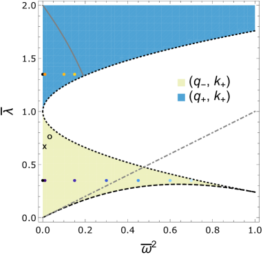
(a) Conical branch ($k=k_{+}$) with sub-critical ($\bar{q}^{2}=\bar{q}^{2}_{-}$) and super-critical ($\bar{q}^{2}=\bar{q}^{2}_{+}$) sub-branch. The dash-dotted line approximates the dashed bound in the decoupling limit.

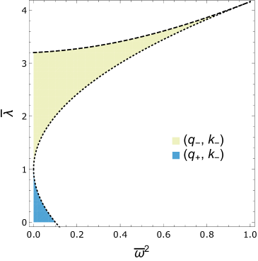
(b) Alternative branch ($k=k_{-}$) with sub-critical ($\bar{q}^{2}=\bar{q}^{2}_{+}$) and super-critical ($\bar{q}^{2}=\bar{q}^{2}_{-}$) sub-branch. It is incompatible with the decoupling limit in (53).

Figure 3: Parameter space of the thin brane model. Each pair $(\bar{\omega},\bar{\lambda})$ corresponds by virtue of (52) to a particular value of $\bar{q}^{2}$ (and to a certain value of $R_{0}$ once the winding number has been fixed). The dotted and dashed lines depict the positivity bound on $A^{2}$ and $\bar{q}^{2}$, respectively. Only the shaded regions admit a stable solution.

In order to ensure a stationnary, real solution, we have to make sure that both $A^{2}$ and $\bar{q}^{2}$ are positive, which is not guaranteed by their respective equations. For $\bar{q}^{2}=\bar{q}^{2}_{-}$ the positivity of $A^{2}$ in (51c) gives an upper bound on $\bar{\lambda}$, and the positivity of $\bar{q}^{2}_{-}$ in (55) gives a lower bound, leaving us with

$$8+3\,\bar{\omega}^{2}-4\,\sqrt{2}\,\sqrt{2-\bar{\omega}^{2}+2\,\bar{\omega}^{4}}<5\,\bar{\lambda}<5-2\,\sqrt{3}\,\sqrt{\left(11-4\,\sqrt{6}\right)}\,|\bar{\omega}|\;,$$ (57)

corresponding to the green (light) shaded region in Fig. 3(a). Note that the upper bound in (56a) is weaker. For ${q}^{2}=\bar{q}^{2}_{+}$ we obtain a lower bound coming from the positivity of $A^{2}$ in (51c)

$$5\,\bar{\lambda}>5+2\,\sqrt{3}\,\sqrt{\left(11-4\,\sqrt{6}\right)}\,|\bar{\omega}|\;,$$ (58)

which again trumps the one in (56b) and gives rise to the blue (dark) shaded region in Fig. 3(a).

The important message is that the $k=k_{+}$ branch admits stationnary solutions with $(\bar{\omega}\neq 0)$ that correspond to a constant brane radius $R_{0}$, and therefore consistently generalises the well-studied static solutions with $\bar{\omega}=0$. The non-shaded regions, on the other hand, are incompatible with a stabilised radius, and we therefore expect them to lead to a run-away behaviour. Moreover, these statements fully take into account the gravitational back-reaction and are hence applicable to cases of sizeable 5D energy densities, corresponding to $\left\{\bar{\lambda},\bar{q}^{2},\bar{\omega}\right\}=\mathcal{O}(1)$, where curvature effects can no longer be neglected. Specifically, without back-reaction we would have excluded the parameter regime below the dashed-dotted line in Fig. 3(a) to ensure positivity of $\bar{q}^{2}$ based on (53), which indeed becomes vastly inaccurate at high energies.

To obtain a better geometrical understanding of this branch, we consider the limit $\bar{\omega}\to 0$. We will find that it is continuously connected to the conical geometry of a static hollow cylinder with constant surface tension, which is characterised by a constant deficit angle $\Delta$. We will henceforth refer to it as the “conical branch” (also for $\bar{\omega}\neq 0$). From (55) and (56) we find that $\bar{q}^{2}=\bar{\lambda}$ for both $\bar{q}^{2}=\bar{q}_{-}^{2}$ and $\bar{q}^{2}=\bar{q}_{+}^{2}$ [which also follows from the decoupling limit in (53)]. We will refer to them as the “sub-critical” and “super-critical” sub-branch as they correspond to the disjoint tension regimes $0<\bar{\lambda}<1$ and $\bar{\lambda}>1$, respectively. Also note that this result is compatible with the decoupling limit in (53), which singles out this branch as the physically relevant one when we want to describe the geometry of a kinky vorton in the thin wall limit.

It is straightforward to check that the integration constants in (42) and (51) reduce to

$$D =1/R_{0}\;, C =0\;, B =1\;,$$

$$F =\left(1-\bar{\lambda}\right)^{-1}\;, E =0\;, A =-1\;.$$ (59)

Note that (51c) also admits the solution $A=1$, which we dismiss as it would imply $C\to\infty$. We further derive $u(r)=1$ and $a(r)=k(r)=0$, leaving us indeed with a conical geometry in the exterior,

$$\mathrm{d}s_{\mathrm{ext}}^{2}=-\mathrm{d}t^{2}+\mathrm{d}\underline{z}^{2}\,+\left(1-\bar{\lambda}\right)^{-2}\mathrm{d}r^{2}\,+\,r^{2}\,\mathrm{d}\varphi^{2}\;,$$ (60)

where the deficit angle is given by $\Delta=2\pi\,\bar{\lambda}$ (see Sec. 3.3 for a more extensive discussion of this geometry). Note that for $F>0$ (sub-critical) the range of $r$ is $[R_{0},\infty)$, whereas for $F<0$ (super-critical) it is $(0,R_{0}]$. In the latter case this implies the existence of a second axis at $r=0$. In summary, the conical branch corresponds to the choice $k=k_{+}$, where its sub-critical and super-critical sub-branch is described by the green (light) and blue (dark) shaded region in Fig. 3(a), respectively.

Alternative branch

Here we briefly discuss the branch with $k=k_{-}$. The solution for $\bar{q}^{2}$ is still given by (55), only the regimes of validity of the respective sub-branches have changed,

$$3\,\bar{\lambda} <3+2\,\sqrt{6}\,|\bar{\omega}|\quad\mathrm{for}\quad\bar{q}^{2}=\bar{q}^{2}_{+}\;,$$ (61a)

$$3\,\bar{\lambda} >3-2\,\sqrt{6}\,|\bar{\omega}|\quad\mathrm{for}\quad\bar{q}^{2}=\bar{q}^{2}_{-}\;.$$ (61b)

As before we demand positivity of $A^{2}$ and $\bar{q}^{2}$, which for $\bar{q}^{2}=\bar{q}^{2}_{-}$ amounts to

$$8+3\,\bar{\omega}^{2}+4\,\sqrt{2}\,\sqrt{2-\bar{\omega}^{2}+2\,\bar{\omega}^{4}}>5\,\bar{\lambda}>5+2\,\sqrt{3}\,\sqrt{\left(11+4\,\sqrt{6}\right)}\,|\bar{\omega}|\;,$$ (62)

corresponding to the green (light) shaded region in Fig. 3(b). For ${q}^{2}=\bar{q}^{2}_{+}$ we obtain the upper bound

$$5\,\bar{\lambda}<5-2\,\sqrt{3}\,\sqrt{\left(11+4\,\sqrt{6}\right)}\,|\bar{\omega}|\;,$$ (63)

giving rise to the blue (dark) shaded region in Fig. 3(b). Like the conical branch, the solution simplifies considerably in the limit $\bar{\omega}\to 0$. Specifically, we obtain the following non-vanishing integration constants: $A=-5$, $\bar{q}^{2}=(16-5\bar{\lambda})/11$ as well as $F=-11/(1-\bar{\lambda})$, which in turn yields the bulk geometry

$$\mathrm{d}s^{2}_{\mathrm{ext}}=\left(\frac{R_{0}}{r}\right)^{4}\,\mathrm{d}t^{2}+\left(\frac{R_{0}}{r}\right)^{4}\,\mathrm{d}\underline{z}^{2}+F^{2}\,\left(\frac{R_{0}}{r}\right)^{12}\,\mathrm{d}r^{2}+r^{2}\,\left(\frac{R_{0}}{r}\right)^{-4}\,\mathrm{d}\varphi^{2}\,.$$ (64)

The existence of this solution had to be expected as a second branch also exists in the (rotationless) 4D case, typically referred to as “Melvin” or “Kasner” branch Linet1990 ; Christensen1999 . However, the solution for $\bar{q}^{2}$ is obviously incompatible with the decoupling limit in (53), so it cannot arise from the microscopic model considered here and hence will not be considered any further.

3.3 Geometry of rotating braneworlds

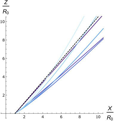
(a) Radial embedding diagram ($Y=0$): rotation leads to a widening of the cone close to the brane. Far away a flat conical profile is approached.

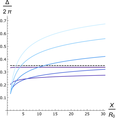
(b) Deficit angle as “seen” by a local bulk observer. Further away curvature decreases and a constant deficit angle is approached.

Figure 4: Deformed cones for sub-critical tension, $\bar{\lambda}=0.35$, and $\bar{\omega}^{2}\in\left\{0.01,0.15,\,0.3,\,0.45,\,0.6,\,0.7\right\}$ [from dark to light, corresponding to the dots in the green (light) region of Fig. 3(a)]. The dashed curve represents the static case ($\bar{\omega}=0$). The brane “sits” at $X=1$.

In order to infer the geometric impact the parameter $\bar{\omega}$ has on the geometry, it is instructive to construct an embedding diagram that visualises the extra space curvature. To that end, we consider a generic extra-dimensional slice of the physical manifold ($\mathrm{d}t=\mathrm{d}\underline{z}=0$),

$$\mathrm{d}s_{\mathrm{ext}}^{2}=F^{2}\,\mathrm{e}^{2\,k(r)}\,\mathrm{d}r^{2}+v(r)^{2}\,\mathrm{d}\varphi^{2}\;,$$ (65)

where we defined

$$v(r)=\sqrt{\frac{r^{2}}{u(r)}-a^{2}(r)\,u(r)}\;.$$ (66)

This metric can be described as a hypersurface in a three-dimensional Euclidian space which is parametrised in terms of $(r,\varphi)$ through the embedding functions $\left[X(r,\varphi),\,Y(r,\varphi),\,Z(r)\right]$, where $X(r,\varphi)=\cos\left(\varphi\right)\,v(r)$, $Y(r,\varphi)=\sin\left(\varphi\right)\,v(r)$ and $Z(r)$ is determined by the boundary value problem

$$Z^{\prime}(r)=\pm\,\sqrt{K^{2}\,\mathrm{e}^{2\,k(r)}-\left[v^{\prime}(r)\right]^{2}}\quad\text{and}\quad Z(R_{0})=0\;.$$ (67)

For $\bar{\omega}=0$ we can use the static geometry in (60). In that case it is easy to solve the differential equation, yielding the embedding

$$\left[X(r,\varphi),\,Y(r,\varphi),\,Z(r)\right]=\left[r\,\cos\left(\varphi\right),\,r\,\sin\left(\varphi\right),\,\pm\,\frac{\sqrt{1-\left(1-\bar{\lambda}\right)^{2}}}{|1-\bar{\lambda}|}\,\left(r-R_{0}\right)\right]\;.$$ (68)

As a further geometrical probe, we introduce the local deficit angle $\Delta(r)$ a 6D observer would infer from two measurements of the bulk circumference at $R$ and $R+\mathrm{d}R$, where $R$ is the proper radius defined by $\mathrm{d}R=\sqrt{g_{rr}}\,\mathrm{d}r$,

$$\frac{\Delta(r)}{2\,\pi}:=1-\frac{\mathrm{d}v(R)}{\mathrm{d}R}=1-\frac{v^{\prime}(r)}{|F|\,\mathrm{e}^{k(r)}}\,.$$ (69)

The second equality follows from (65). Evaluated at the brane, we obtain

$$\frac{\Delta(r)}{2\,\pi}=1\mp\left[1-\frac{1}{8}\,\left(\bar{\omega}^{2}+7\,\bar{q}^{2}_{\mp}+\bar{\lambda}\right)\right]\,,$$ (70)

where we used (66) and (45). In the static case ($\bar{\omega}=0\Rightarrow\bar{q}^{2}=\bar{\lambda}$) this reduces to $\Delta(r)/(2\pi)=1-|1-\bar{\lambda}|$, which agrees with the well-known expression for a global deficit angle.

Sub-critical tension

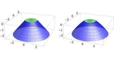
(a) Sub-critical tension ($\bar{\lambda}=0.35$). Without rotation ($\bar{\omega}^{2}=0$, left) the extra space is a flat cone. With rotation ($\bar{\omega}^{2}=0.45$, right) we observe a slight widening of the cone and a build-up of curvature close to the brane.

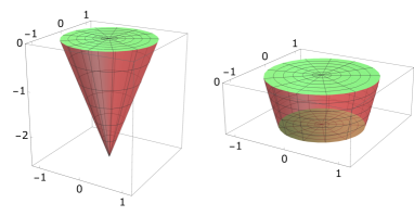
(b) Super-critical tension ($\bar{\lambda}=1.35$): Without rotation ($\bar{\omega}^{2}=0$, left) the extra space is an inverted cone that closes in a conical singularity. With rotation ($\bar{\omega}^{2}=0.001$, right) the extra space is capped at $r=0.65$ (“o”) before an excess develops.

Figure 5: Embedding diagrams of the extra space geometry. The interior (green) is flat whereas the exterior (blue or red) features a conical deficit and is curved for $\bar{\omega}\neq 0$.

We first discuss the geometry of a sub-critical tension brane ($\bar{\lambda}<1$). In the static case ($\bar{\omega}=0$) the extra space is described by a (constant) conical geometry with vanishing curvature. The corresponding embedding diagramm (for $Y=0$) and deficit angle are depicted as the dashed line in Fig. 4(a) and 4(b), respectively (see also Fig. 5(a) for the full angular embedding). This is the higher dimensional generalisation of the geometry of an infinitely long, straight cosmic string in 4D Vilenkin1981c ; Gott1985 ; Hiscock1985a . For $\bar{\omega}\neq 0$ we integrate (67) numerically and evaluate (69) to obtain the coloured lines in Fig. 4(a) and 4(b), respectively. We see that the angular momentum of the brane leads to a widening of the cone close to the brane. Contrary to the static case, the bulk spacetime is no longer flat, it rather has non-vanishing spatial curvature which becomes strongest in the near-brane region and falls off as $r\to\infty$. Accordingly, the bulk curves into a constant cone far way from the brane. Fig. 4(b) shows that the asymptotic deficit angle can lie above (for large $\bar{\omega}$) or below (for small $\bar{\omega}$) the static value. Further, from the parameter plot in Fig. 3(a) it follows that in order to realise a deficit angle that asymptotes to a near-critical value ($\Delta\lesssim 2\pi$) we either have to tune $\bar{\lambda}\lesssim 1$ and $\bar{\omega}\ll 1$ (which is close to the well-studied static case) or occupy the green (light) sliver around $\bar{\lambda}\approx 0.2$ which admits $\bar{\omega}\lesssim 1$ (best approximated by the lightest blue line in Fig. 3(a)).

Another crucial observation is that the intrinsic brane geometry is flat for all consistent parameter choices, which is obvious from the induced metric in (40). This implies that the self-tuning (or degravitation) property, which makes 6D braneworld models interesting with respect to the cosmological constant problem, is preserved for our (sub-critical) kinky vorton model (see for example Niedermann:2014bqa and references therein).

Super-critical tension

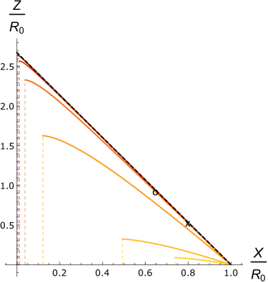
(a) Radial embedding diagram ($Y=0$): rotation leads to a wider inverted cone. To avoid an excess angle, the extra space has to be capped by a second (sub-critical) brane sitting to the right of the dashed line.

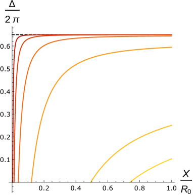
(b) The local deficit angle decreases away from the brane until it turns eventually negative, corresponding to an excess angle.

Figure 6: Deformed inverted cones for super-critical tension, $\bar{\lambda}=1.35$, and $\bar{\omega}^{2}\in\left\{10^{-5},10^{-4},\,10^{-3},\,10^{-2},\,10^{-1},\,0.15\right\}$ [from dark to light, corresponding to the dots in the blue (dark) region in Fig. 3(a)]. The dashed curve represents the static case ($\bar{\omega}=0$). The brane “sits” at $X=1$.

In the super-critical case when $\bar{\lambda}>1$ the circumference of the extra space shrinks as we move away from the brane. In the static case, this leads to an inverted cone with deficit angle $\Delta/(2\pi)=2-\bar{\lambda}$, which closes in a second axis Ortiz:1990tn ; Blanco-Pillado2014 (at coordinate position $r=0$), depicted by the dashed lines in Fig. 6 (see also Fig. 5(b) for the full angular embedding). As this additional axis exhibits a conical singularity, it signals the presence of second brane with fine-tuned tension $\bar{\lambda}_{*}=2-\bar{\lambda}$. This brane can either be infinitely thin, giving rise to the observed singularity, or again be described in terms of an extended configuration, smoothing out the singularity. In the latter case the bulk is “capped” at some non-vanishing value $0<r_{2}<R_{0}$. In both cases the bulk spacetime becomes compact.

We now move on to the rotating case. We find that the (inverted) cone is generically widened as we increase $\bar{\omega}$, cf. Fig. 6(a). Moreover, this effect gets more pronounced the further we move away from the brane (the smaller $X$ or $r$ is), and is accompanied by a build-up of spatial curvature. This resonates with the observation that the curves in Fig. 6(b) become steeper as we approach the axis at $X=0$. Eventually, it drops below zero that way indicating the presence of an excess angle (rather than a deficit angle). This point is marked by the (vertical) dashed lines in Fig. 6(a). However, as excess angles generically require a negative brane tension, we dismiss this regime as unphysical (at least it cannot be described in terms of the kinky vorton model proposed here). We therefore require the bulk spacetime to be regularised before that point is reached, which again can be achieved by including a second brane, cf. right plot in Fig. 5(b). Its stress-energy has to be tuned such that it gives rise to the correct value of $\Delta(X)$ at its position. We will provide an explicit example later in Sec. 3.5. We also see from Fig. 6(b) that the point where $\Delta(X)$ drops below zero moves further to the brane for larger values of $\bar{\omega}$. This implies that there is a maximal $\bar{\omega}$ for which it is no longer possible to regularise the bulk in terms of a physical, i.e. non-negative, brane tension. By demanding $\Delta(R_{0})>0$ we derive from (69) the bound

$$6\,\bar{\lambda}<-2+8\,\bar{\omega}^{2}+7\,\sqrt{2}\,\sqrt{2-7\,\bar{\omega}^{2}+2\,\bar{\omega}^{4}}\;,$$ (71)

which is depicted as the grey curve in the blue (dark) region in Fig. 3(a). We thus find that the extra space cone becomes shorter for larger values of $\bar{\omega}$ due to the necessity of capping the space earlier.

In summary, super-critical solutions ($\bar{\lambda}>1$) can be consistently generalised to $\bar{\omega}\neq 0$ by introducing a second sub-critical brane which caps the extra space at a finite distance away from the axis at $X=0$. We further find that rotation leads to a widening and shortening of the inverted cone.

3.4 Dragging of inertial frames

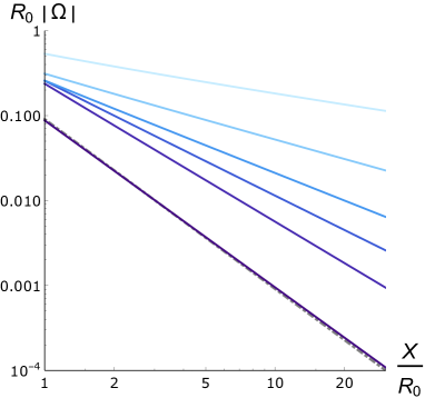
(a) Sub-critical case (static frame): The angular momentum of the brane (proportional to $\bar{\omega}$) drags along the bulk spacetime with diminishing effect as we move further away.

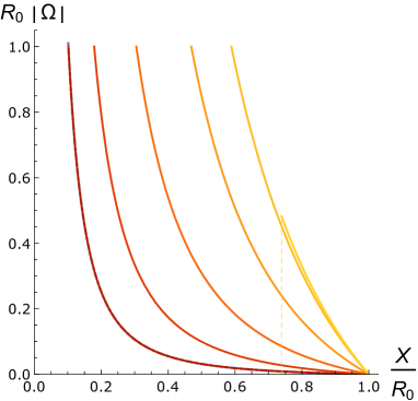
(b) Super-critical case (co-rotating frame): The “dragging” of the exterior space increases for larger angular momentum of the brane.

Figure 7: Radial profile of the rotation function $\Omega(r)$ with parameter values and color coding ($\bar{\omega}$ increasing from dark to light) as specified in Fig. 4 and Fig. 6, respectively. The dashed-dotted lines correspond to the analytic result in the slowly rotating case.

The main new physical feature we introduce in this paper is an angular momentum of the brane, cf. Eq. (28). Here we discuss how this property affects the relative angular motion of different inertial bulk observers. We first discuss the sub-critical case for which the bulk is infinite.

We start with the coordinate transformation

$$\tilde{\varphi}=\varphi+\Omega_{0}\,t,$$ (72)

where $\Omega_{0}$ is constant. The metric (34) then reads

$$\mathrm{d}s^{2}_{\mathrm{ext}}=-r^{2}\,v(r)^{-2}\,\mathrm{d}t^{2}+\mathrm{e}^{2\,k(r)/3}\mathrm{d}\underline{z}^{2}+F^{2}\,\mathrm{e}^{2\,k(r)}\mathrm{d}r^{2}+v(r)^{2}\left[\mathrm{d}\tilde{\varphi}-\Omega(r)\mathrm{d}t\right]^{2}\;,$$ (73)

where $v(r)$ has been defined in (66). We also identified the $r$-dependent function

$$\Omega(r) =\Omega_{0}+\frac{a(r)\,u(r)}{v(r)^{2}}\;.$$ (74)

We further fix the constant $\Omega_{0}$ by demanding $\lim_{r\to\infty}\,\Omega(r)=0$, explicitly

$$\Omega_{0} =-\,\lim_{r\to\infty}\frac{a(r)\,u(r)}{v(r)^{2}}$$

$$=E\,\frac{\left[A-\sqrt{A^{2}+4\,R_{0}^{2}\,E^{2}}\right]^{2}-4\,R_{0}^{2}\,E^{2}}{\left(-A\right)\,\left[A-\sqrt{A^{2}+4\,R_{0}^{2}\,E^{2}}\right]^{2}}\;,$$ (75)

where the second line assumes the conical branch.

We will now argue that $\Omega(r)$ provides a sensible measure of the “rotation of spacetime”. To that end, we consider a slowly rotating brane, corresponding to

$$R_{0}\,E\,\approx\,\sqrt{\bar{\lambda}}\,\left(1-\bar{\lambda}\right)^{-1}\,\bar{\omega}\ll 1\;.$$ (76)

At linear order in $E$ we find $A\approx-1$, $B\approx 1$, $C\approx R_{0}^{2}\,E$ as well as $\Omega_{0}\approx E$ due to (3.4). Substituting these into Eqs. (36) and (37) yields $v(r)\approx r$ and $k(r)\approx 0$, which in turn implies

$$\mathrm{d}s^{2}_{\mathrm{ext}}\approx-\,\mathrm{d}t^{2}+\mathrm{d}\underline{z}^{2}+F^{2}\mathrm{d}r^{2}+r^{2}\left[\mathrm{d}\tilde{\varphi}-\Omega(r)\mathrm{d}t\right]^{2}\;,$$ (77)

where due to (74)

$$\Omega(r)\approx\frac{R_{0}^{2}}{r^{2}}\,\Omega_{0}\approx\frac{R_{0}}{r^{2}}\,\sqrt{\bar{\lambda}}\,\left(1-\bar{\lambda}\right)^{-1}\,\bar{\omega}\,.$$ (78)

We indeed find that $\Omega(r)$ vanishes in the limit $r\to\infty$, leading to a non-rotating and locally flat Minkowski metric. The $(t,\tilde{\varphi})$-frame hence corresponds to a static, inertial observer at radial infinity (residing at constant $\tilde{\varphi}$) and thus sets the standard of no rotation. The $(t,\varphi)$-frame, on the other hand, corresponds to an inertial observer at the brane (residing at constant $\varphi$). Due to (72) [or (78)], it rotates with respect to the asymptotic observer with angular velocity $\Omega_{0}$. The function $\Omega(r)$ generalizes this concept to intermediate observers at radius $R_{0}\leq r<\infty$ and, in that particular sense, corresponds to the “rotation of spacetime”.

Eq. (78) suggests that the rotation is enhanced when the brane tension approaches the critical value $\bar{\lambda}=1$. However, from the parameter plot in Fig. 3(a) it is clear that this limit is only consistent if we sent $\bar{\omega}\to 0$ which counteracts the enhancement. On the other hand, in the limit where the brane tension is sent to zero ($\lambda\to 0$), all gravitational effects of the brane disappear, leading to an empty 6D Minkowski spacetime without rotation.

We now depart from the limit of slow rotation and evaluate the function $\Omega(r)$ for different values of $\bar{\omega}$ in Fig. 7(a), assuming that it still provides a sensible measure of rotation. We find a power law behavior $\Omega(X)\propto X^{-\alpha}$ with $0<\alpha<2$, where the upper limit is approached for a slowly rotating brane in accordance with (78) (dash-dotted line). We also see that $\Omega$ becomes generically larger, when $\bar{\omega}$ is increased. This nicely resonates with the observation that the angular momentum of the brane, as defined in the decoupling limit in (28), is proportional to $\bar{\omega}$.

In the super-critical case ($\bar{\lambda}>0$), the extra space is compact which prevents us from introducing an inertial frame at radial infinity. We therefore use the super-critical brane as the non-rotating reference point with respect to which inertial bulk observers are rotating with angular velocity

$$\tilde{\Omega}(r) =-\frac{a(r)\,u(r)}{v(r)^{2}}\;.$$ (79)

Note the constant shift in comparison to (74). The function $\tilde{\Omega}(X)$ is depicted in Fig. 7(b) for different values of $\bar{\omega}$. Starting with the hierarchically small value $\bar{\omega}=10^{-5}$, we find that increasing $\bar{\omega}$ leads to an increase in $\tilde{\Omega}(X)$ for all values of $X$, again in accordance with its interpretation as the rotation of spacetime. All curves diverge towards $X=0$. Note however that spacetime has to be cut off before $X=0$ is reached to avoid an excess angle (for $\bar{\omega}=0.15$ the “excess point” is marked by the dashed line).

In summary, we have argued (and explicitly shown for a slowly rotating brane) that due to the angular momentum of the brane, inertial observers at different radial positions are rotating with respect to each other. This effect, known as the dragging of inertial frames in the context of rotating black holes, is controlled by the value of $\bar{\omega}$.

3.5 Second brane matching

We have seen that for a super-critical brane the extra space needs to be capped by including a second sub-critical brane, otherwise a regime of (diverging) excess angle close to the symmetry axis occurs. The crucial question is whether such a brane exists, i.e. can be realized in terms of a physical matter theory. Our analysis allows us to answer this question, at least if we again employ the thin vorton model to describe the second brane. To be specific, for every point, $\left(\bar{\omega}^{2},\,\bar{\lambda}\right)$, in the blue (dark) parameter regime in Fig. 3(a) (corresponding to the super-critical brane) and a given radial position $r_{*}<R_{0}$, we can ask whether there exists a dual point, $\left(\bar{\omega}^{2}_{*},\,\bar{\lambda}_{*}\right)$, in the green (light) region (corresponding to a sub-critical brane that consistently caps the extra space at $r=r_{*}$).

We first note that for a given branch choice the bulk geometry is fully determined once the parameters $\bar{\omega}^{2}$ and $\bar{\lambda}$ have been fixed. It is therefore enough to match two geometric quantities in order to fix the matter content of the dual brane. Here we will employ the deficit angle, $\Delta(r)$, and the rotational profile, $\tilde{\Omega}(r)$. The former is given by (69) and can be (numerically) evaluated at $r=r_{*}$ for a given choice of $\bar{\omega}^{2}$ and $\bar{\lambda}$; on the other hand, it is also related to the matter content on the second brane according to (70) subject to the formal replacement $\left\{\bar{\omega}^{2},\bar{\lambda}\right\}\to\left\{\bar{\omega}^{2}_{*},\,\bar{\lambda}_{*}\right\}$. Applying the same reasoning to $R_{0}^{2}\,\tilde{\Omega}^{\prime}(r)$ as defined in (79), we obtain the two matching equations

$$\frac{1}{8}\,\left(\bar{\omega}^{2}_{*}+7\,\bar{q}^{2}_{*}+\bar{\lambda}_{*}\right)\, \stackrel{{\scriptstyle!}}{{=}}\,\frac{\Delta(r_{*})}{2\pi}\,,$$ (80a)

$$\frac{-8\,\bar{q}_{*}\,\bar{\omega}_{*}}{4-3\,\bar{q}_{*}^{2}-\bar{\lambda}_{*}+3\,\bar{\omega^{2}_{*}}}\, \stackrel{{\scriptstyle!}}{{=}}\,R_{0}^{2}\,\tilde{\Omega}^{\prime}(r_{*})\;,$$ (80b)

where $\bar{q}^{2}_{*}(\bar{\omega}_{*},\bar{\lambda}_{*})$ is determined by the “ – ” branch in (55), corresponding to a sub-critical brane. Note that we used $\tilde{\Omega}^{\prime}(r)$ [rather than $\tilde{\Omega}(r)$] as this quantity does not depend on the choice of the non-rotating reference frame. As a check of these relations we can consider the static limit ($\bar{\omega}=0$), which implies $\bar{\omega}_{*}=0$ and the tuning-relation $\bar{\lambda}_{*}=2-\bar{\lambda}$ in agreement with the literature Blanco-Pillado2014 . The authors in Ref. Niedermann:2014yka investigated what happens in cases where the brane tensions do not fulfil the above relation, and it was found that stationary solutions exist for which the brane starts to expand in axial direction with constant rate, corresponding to a 4D de Sitter phase on the brane. As our ansatz in (34) is not general enough to accommodate an expanding brane, we remain short on a definite statement about the rotating brane case. However, it is conceivable that there is a continuously connected super-critical solution with $\bar{\omega}\neq 0$ which shows the same inflating behaviour.

Here we do not provide an exhaustive discussion of the matching and rather present a proof of existence relying on a special choice of parameters. Specifically, we use

$$\bar{\lambda}\,=\,1.35\,, \bar{\omega}^{2}\,=\,0.001\,,$$ (81)

corresponding to one of the super-critical solutions depicted in Fig. 6. We further consider the two radii $r_{*}/R_{0}\in\left\{0.65,\,0.8\right\}$ at which we cap the extra space, marked by the points “o” and “x” in Fig. 6(a) (see also the right plot in Fig. 5(b)). With this choice we can calculate the right side of Eqs. (80). We then use a numerical root finding algorithm to determine the corresponding points in the $\left(\bar{\omega}^{2}_{*},\,\bar{\lambda}_{*}\right)$-plane, depicted by “x” and “o” in Fig. 3(a). And indeed we find that both are within the green (light) shaded region, representing consistent, stationary (non-inflating) configurations of the super-critical system. Let us stress that those solutions are particularly interesting for model building purposes as they correspond to compact extra dimensions, admitting a 4D gravity regime at low energy scales.

4 Conclusions

In this paper we have examined a microphysical model that could lead (or be extended) to established 6D braneworlds of finite Peloso:2006cq ; Aghababaie:2003wz ; Niedermann:2014yka or infinite Dvali:2000xg ; Kaloper:2007ap extra space volume, whereby two extra dimensions are hidden by having the Universe live on a cylindrical brane. In the existing construction, which used a thin-wall approach to the calculation, the brane had a massless, periodic scalar field living inside its worldvolume, and the cylindrical brane was prevented from collapsing by a winding of the worldvolume scalar. From the perspective of the microscopic model used here, this thin-wall approach removes degrees of freedom, which turns out to be crucial. Indeed, there are unstable modes in the microphysics that break the rotational symmetry of the extra dimensions, questioning the UV stability of this particular incarnation of braneworlds. However, using the same model it is possible to fix the problem. Taking a lesson from the cosmology of topological defects known as vortons Davis:1988jq ; Davis:1988ip ; Davis:1988ij , we learn that rotation of the ring-like object is crucial to prevent its collapse. In the context of the underlying microphysics, or indeed the worldvolume theory, this corresponds to having a current circulate around the loop, rather than simply a winding number.

By using the analytic properties of a field theory model, spelled out in Battye:2008zh ; Battye:2009nf , we have taken parameters from the microscopic model where the flat-space ring solutions are known to be stable (under axially symmetric perturbations), and placed them in a gravitational setting, using a thin-wall approximation. The extra freedom of rotation gives a richer set of braneworld solutions, where the rotating braneworld drags the ambient spacetime along with it. We have explored a range of parameters and have found that in cases where the deficit angle in the extra dimensions is less than $2\pi$ (sub-critical) we have infinite volume in the extra dimensions, whilst for larger deficit angles (super-critical) the extra dimensions are compact. The former set could be easily extended to the BIG model Kaloper:2007ap by adding a four dimensional Einstein Hilbert term to the worldvolume theory in (33). In fact, this would not change the vacuum configurations as they correspond to vanishing intrinsic brane curvature. It would then be interesting whether the new freedom due to rotation helps to avoid the ghost instabilities diagnosed within the same cylindrical brane setup in Niedermann:2014bqa ; Eglseer:2015xla . Note that, according to the findings in Niedermann:2017cel , this would require a screening mechanism (for example Vainshtein screening Vainshtein:1972sx ) to kick in at small distance scales. On the other hand, the latter set offers, due to its compactness, a different type of interesting phenomenology. This could be further explored by generalizing from a Minkowski worldvolume geometry to a cosmological setting, just as was done for the cigar shaped proposal in the non-rotating case Niedermann:2014yka . Regarding the stability of our rotating configurations, a final statement still requires a study of non-axially symmetric perturbations. A similar fluctuation analysis would also allow to infer the phenomenological implications of the presence of the scalar degree of freedom $\tilde{\sigma}$, which so far has only been investigated in the non-rotating case in Kaloper:2007ap ; Eglseer:2015xla .

As a final speculation we would like to comment on the effect that rotation has on fermions bound to the braneworld. In practise, the braneworld has non-zero thickness, and the braneworld matter fields have wavefunctions that peak somewhere on the brane. The precise location of the wavefunctions of the different fermions has important consequences for the fermion mass hierarchy, and proton stability, as pointed out by ArkaniHamed:1998sj ; ArkaniHamed:1999dc . This is due to the overlap between different wavefunctions being exponentially suppressed as their centres move away from one another. In the context of our spinning cylindrical braneworld it is natural to expect the heavier braneworld fermions to be pushed to a larger radius than the lighter ones, and so could give a natural description of this mechanism. This would, of course, require a full calculation to give concrete realisation.

- (1) Y. B. Zel’dovich, Cosmological Constant and Elementary Particles, JETP Lett. 6 (1967) 316.
- (2) Ya. B. Zel’dovich, A. Krasinski and Ya. B. Zeldovich, The Cosmological constant and the theory of elementary particles, Sov. Phys. Usp. 11 (1968) 381–393.
- (3) S. Weinberg, The Cosmological Constant Problem, Rev. Mod. Phys. 61 (1989) 1–23.
- (4) C. P. Burgess, The Cosmological Constant Problem: Why it’s hard to get Dark Energy from Micro-physics, in Proceedings, 100th Les Houches Summer School: Post-Planck Cosmology: Les Houches, France, July 8 - August 2, 2013, pp. 149–197, 2015, 1309.4133, DOI.
- (5) A. Padilla, Lectures on the Cosmological Constant Problem, 1502.05296.
- (6) G. R. Dvali and G. Gabadadze, Gravity on a brane in infinite volume extra space, Phys. Rev. D63 (2001) 065007, [hep-th/0008054].
- (7) N. Kaloper and D. Kiley, Charting the landscape of modified gravity, JHEP 05 (2007) 045, [hep-th/0703190].
- (8) G. R. Dvali, G. Gabadadze and M. Porrati, 4-D gravity on a brane in 5-D Minkowski space, Phys. Lett. B485 (2000) 208–214, [hep-th/0005016].
- (9) S. L. Dubovsky and V. A. Rubakov, Brane induced gravity in more than one extra dimensions: Violation of equivalence principle and ghost, Phys. Rev. D67 (2003) 104014, [hep-th/0212222].
- (10) S. F. Hassan, S. Hofmann and M. von Strauss, Brane Induced Gravity, its Ghost and the Cosmological Constant Problem, JCAP 1101 (2011) 020, [1007.1263].
- (11) F. Niedermann, R. Schneider, S. Hofmann and J. Khoury, Universe as a cosmic string, Phys. Rev. D 91 (2015) 024002, [1410.0700].
- (12) L. Eglseer, F. Niedermann and R. Schneider, Brane induced gravity: Ghosts and naturalness, Phys. Rev. D92 (2015) 084029, [1506.02666].
- (13) F. Niedermann and A. Padilla, Gravitational Mechanisms to Self-Tune the Cosmological Constant: Obstructions and Ways Forward, Phys. Rev. Lett. 119 (2017) 251306, [1706.04778].
- (14) N. Arkani-Hamed, S. Dimopoulos and G. R. Dvali, The Hierarchy problem and new dimensions at a millimeter, Phys. Lett. B429 (1998) 263–272, [hep-ph/9803315].
- (15) I. Antoniadis, N. Arkani-Hamed, S. Dimopoulos and G. R. Dvali, New dimensions at a millimeter to a Fermi and superstrings at a TeV, Phys. Lett. B436 (1998) 257–263, [hep-ph/9804398].
- (16) Y. Aghababaie, C. P. Burgess, S. L. Parameswaran and F. Quevedo, Towards a naturally small cosmological constant from branes in 6-D supergravity, Nucl. Phys. B680 (2004) 389–414, [hep-th/0304256].
- (17) G. W. Gibbons, R. Gueven and C. N. Pope, 3-branes and uniqueness of the Salam-Sezgin vacuum, Phys. Lett. B595 (2004) 498–504, [hep-th/0307238].
- (18) C. P. Burgess and L. van Nierop, Large Dimensions and Small Curvatures from Supersymmetric Brane Back-reaction, JHEP 04 (2011) 078, [1101.0152].
- (19) C. P. Burgess and L. van Nierop, Technically Natural Cosmological Constant From Supersymmetric 6D Brane Backreaction, Phys. Dark Univ. 2 (2013) 1–16, [1108.0345].
- (20) F. Niedermann and R. Schneider, Fine-tuning with brane-localized flux in 6D supergravity, JHEP 02 (2016) 025, [1508.01124].
- (21) F. Niedermann and R. Schneider, SLED phenomenology: curvature vs. volume, JHEP 03 (2016) 130.
- (22) L. Randall and R. Sundrum, A Large mass hierarchy from a small extra dimension, Phys. Rev. Lett. 83 (1999) 3370–3373, [hep-ph/9905221].
- (23) L. Randall and R. Sundrum, An Alternative to compactification, Phys. Rev. Lett. 83 (1999) 4690–4693, [hep-th/9906064].
- (24) R. Maartens and K. Koyama, Brane-World Gravity, Living Rev. Rel. 13 (2010) 5, [1004.3962].
- (25) F. Niedermann and R. Schneider, Radially stabilized inflating cosmic strings, Phys. Rev. D 91 (2015) 064010, [1412.2750].
- (26) J. Vinet and J. M. Cline, Can codimension-two branes solve the cosmological constant problem?, Phys. Rev. D70 (2004) 083514, [hep-th/0406141].
- (27) H. B. Nielsen and P. Olesen, Vortex Line Models for Dual Strings, Nucl. Phys. B61 (1973) 45–61.
- (28) C. P. Burgess, R. Diener and M. Williams, The Gravity of Dark Vortices: Effective Field Theory for Branes and Strings Carrying Localized Flux, JHEP 11 (2015) 049, [1506.08095].
- (29) C. P. Burgess, R. Diener and M. Williams, EFT for Vortices with Dilaton-dependent Localized Flux, JHEP 11 (2015) 054, [1508.00856].
- (30) W. Israel, Singular hypersurfaces and thin shells in general relativity, Nuovo Cim. B44S10 (1966) 1.
- (31) M. Peloso, L. Sorbo and G. Tasinato, Standard 4-D gravity on a brane in six dimensional flux compactifications, Phys. Rev. D73 (2006) 104025, [hep-th/0603026].
- (32) C. P. Burgess, D. Hoover, C. de Rham and G. Tasinato, Effective Field Theories and Matching for Codimension-2 Branes, JHEP 03 (2009) 124, [0812.3820].
- (33) F. Niedermann and R. Schneider, Cosmology on a cosmic ring, JCAP 1503 (2015) 050, [1411.3328].
- (34) R. A. Battye and P. M. Sutcliffe, Kinky Vortons, Nucl. Phys. B805 (2008) 287–304, [0806.2212].
- (35) R. A. Battye, J. A. Pearson, S. Pike and P. M. Sutcliffe, Formation and evolution of kinky vortons, JCAP 0909 (2009) 039, [0908.1865].
- (36) R. A. Battye and P. M. Sutcliffe, Stability and the equation of state for kinky vortons, Phys. Rev. D80 (2009) 085024, [0908.1344].
- (37) R. Davis and E. P. S. Shellard, The physics of vortex superconductivity. ii, Physics Letters B 209 (1988) 485–490.
- (38) J. P. Ostriker, A. C. Thompson and E. Witten, Cosmological Effects of Superconducting Strings, Phys. Lett. B180 (1986) 231–239.
- (39) E. J. Copeland, N. Turok and M. Hindmarsh, Dynamics of Superconducting Cosmic Strings, Phys. Rev. Lett. 58 (1987) 1910–1913.
- (40) D. Haws, M. Hindmarsh and N. Turok, SUPERCONDUCTING STRINGS OR SPRINGS?, Phys. Lett. B209 (1988) 255–261.
- (41) E. Copeland, D. Haws, M. Hindmarsh and N. Turok, Dynamics of and radiation from superconducting strings and springs, Nuclear Physics B 306 (1988) 908–930.
- (42) R. L. Davis, SEMITOPOLOGICAL SOLITONS, Phys. Rev. D38 (1988) 3722.
- (43) R. L. Davis and E. P. S. Shellard, COSMIC VORTONS, Nucl. Phys. B323 (1989) 209–224.
- (44) H. Davies and T. Caplan, The space-time metric inside a rotating cylinder, in Proc. Camb. Phil. Soc, vol. 69, p. 325, 1971.
- (45) H. Levy and W. J. Robinson, The rotating body problem, Mathematical Proceedings of the Cambridge Philosophical Society 60 (1964) 279–285.
- (46) E. Frehland, The general stationary gravitational vacuum field of cylindrical symmetry, Commun. Math. Phys. 23 (1971) 127–131.
- (47) E. Kasner, Solutions of the einstein equations involving functions of only one variable, Transactions of the American Mathematical Society 27 (1925) 155–162.
- (48) B. Linet, On the supermassive U(1) gauge cosmic strings, Class. Quant. Grav. 7 (1990) L75–L79.
- (49) M. Christensen, A. L. Larsen and Y. Verbin, Complete classification of the string - like solutions of the gravitating Abelian Higgs model, Phys. Rev. D60 (1999) 125012, [gr-qc/9904049].
- (50) A. Vilenkin, Gravitational Field of Vacuum Domain Walls and Strings, Phys. Rev. D23 (1981) 852–857.
- (51) J. R. Gott, III, Gravitational lensing effects of vacuum strings: Exact solutions, Astrophys. J. 288 (1985) 422–427.
- (52) W. A. Hiscock, Exact Gravitational Field of a String, Phys. Rev. D31 (1985) 3288–3290.
- (53) M. E. Ortiz, A New look at supermassive cosmic strings, Phys. Rev. D 43 (1991) 2521–2526.
- (54) J. J. Blanco-Pillado, B. Reina, K. Sousa and J. Urrestilla, Supermassive Cosmic String Compactifications, JCAP 1406 (2014) 001, [1312.5441].
- (55) A. I. Vainshtein, To the problem of nonvanishing gravitation mass, Phys. Lett. 39B (1972) 393–394.
- (56) N. Arkani-Hamed and S. Dimopoulos, New origin for approximate symmetries from distant breaking in extra dimensions, Phys. Rev. D65 (2002) 052003, [hep-ph/9811353].
- (57) N. Arkani-Hamed and M. Schmaltz, Hierarchies without symmetries from extra dimensions, Phys. Rev. D61 (2000) 033005, [hep-ph/9903417].