Social Event Scheduling ^⋆

Abstract

A major challenge for social event organizers (e.g., event planning and marketing companies, venues) is attracting the maximum number of participants, since it has great impact on the success of the event, and, consequently, the expected gains (e.g., revenue, artist/brand publicity). In this paper, we introduce the Social Event Scheduling (SES) problem, which schedules a set of social events considering user preferences and behavior, events’ spatiotemporal conflicts, and competing events, in order to maximize the overall number of attendees. We show that SES is strongly NP-hard, even in highly restricted instances. To cope with the hardness of the SES problem we design a greedy approximation algorithm. Finally, we evaluate our method experimentally using a dataset from the Meetup event-based social network.

I Introduction

The wide adoption of social media and networks has recently given rise to a new type of social networks that focus on online event management, called Event-based Social Networks (EBSN) [7]. In the most predominant EBSN platforms, such as Meetup, Eventbrite or Whova, users organize, manage and share social events and activities. In conjunction with the events’ organizers in EBSNs, several entities such as event planning and marketing companies (e.g., Jack Morton, GPJ), organizations (e.g., IEEE), as well as venues (e.g., theaters, night clubs), organize and manage a variety of social events (music concerts, conferences, promotion parties). A major challenge for event organizers is attracting the maximum number of participants, since it has great impact on the success of the event, and consequently, on the expected gains from it, for all involved (e.g., revenue, artist/brand publicity).

Consider the following real-world scenario. A company is going to organize the Summerfest festival. Summerfest is an 11-day music festival, featuring 11 stages and attracting more than 800K people each year. Throughout the festival, in addition to the music concerts, numerous multi-themed events take place (e.g., theatrical performances). Assume that Alice enjoys listening to Pop music, and is a fashion lover. On Monday from 7:00 to 10:00pm, a concert of a famous Pop band is scheduled to take place at the festival. At the same day, on a different stage, a fashion show is taking place from 7:00 to 9:00pm. Furthermore, from 6:00 to 8:00pm on that day, a music concert of a Pop singer has been organized by a nearby (competing) venue. Despite the fact that Alice is interested in all three events, she is only able to attend one of them. In another scenario, assume that a Pop concert is hosted by the festival on Tuesday evening, but Alice is not capable of attending this event, because on Tuesdays she works until late at night.

The above example illustrates the major aspects that should be considered in events scheduling scenarios. In order to attract as many attendances as possible, organizers have to carefully select the events that are going to take place during the festival, possibly picking among from numerous candidate events, as well as the date/time on which each event is going to take place. During the event scheduling process, at least the following aspects have to be considered: user preferences, user habits (e.g., availability), spatiotemporal conflicts between scheduled events, and possible third parties events (e.g., organized by a third party company) which might attract potential attendees (i.e., competing events).

In this work, we introduce the Social Event Scheduling (SES) problem, which considers the aforementioned aspects and the goal is to maximize the overall number of participants in the scheduled events. In short, given a set of events, a set of time periods and a set of users, our objective is to determine how to assign events on the time periods, so that the maximum participant enrollment is achieved.

Recently, a number of works have been proposed in the context of event-participant planing [6, 12, 13, 11, 15, 14, 5, 2]. These works examine a problem from a different perspective: given a set of pre-scheduled events, they focus on finding the most appropriate assignments for the users (i.e., participants) attending the events. The determined user-event assignments aim at maximizing the satisfaction of the users. However, these works fail to consider a crucial issue in event management, which is the “satisfaction” (e.g., revenue, publicity) of the entities involved in the event organization (e.g., organizer, artist, sponsors, services’ providers). Here, in contrast to existing works, our objective is to maximize the satisfaction of the event-side entities. To this end, instead of assigning users to events, we assign events to time intervals, so that the number of events’ attendees is maximized. Briefly, we study an “event-centric” problem, while the existing approaches focus on “user-centric” problems.

Therefore, our objective is substantially different compared to the existing works. The same holds for the solution; in our problem, the solution is a set of event-time assignments, while in existing works is a set of user-event assignments. Additionally, in order to solve our problem we have to find a subset from a set of candidate events (i.e., some events may not be included in the solution), while in other works the solution contains all the users (i.e., each user is assigned to events). Finally, beyond the user and event entities which are also considered in existing works, in our problem more core entities are involved (e.g., event organizer, competing events). Thus, overall, the objective, the solution and the setting of our problem substantially differ from existing works.

II Social Event Scheduling Problem

In this section we first introduce the Social Event Scheduling (SES) problem; and then we study its complexity. Before we formally introduce our problem, we present some necessary definitions.

Organizer & Time intervals. We assume that the event organizer (e.g., company, venue) is associated with a number of (available) resources $\theta\in\mathbb{R}^{+}$. For example, as resources we can consider the agents (i.e., staff) which are responsible to setup and coordinate the events. Let $\mathcal{T}$ be a set of candidate time intervals, representing time periods that are available for organizing events. Note that the intervals contained in $\mathcal{T}$ are disjoint.

Candidate Events. Assume a set $\mathcal{E}$ of available events to be scheduled, referred as candidate events. Each $e\in\mathcal{E}$ is associated with a location $\ell_{e}$ representing the place (e.g., a stage) that is going to host the event. Further, each event $e$ requires a specific amount of resources $\xi_{e}\in\mathbb{R}^{+}_{0}$ for its organization, referred as required resources.

Schedule & Assignment. An assignment $\alpha_{e}^{t}$ denotes that the candidate event $e\in\mathcal{E}$ is scheduled to take place at $t\in\mathcal{T}$. An event schedule ${\mathcal{S}}$ is a set of assignments, where there exist no two assignments referring to the same event. Given a schedule $\mathcal{S}$, we denote as $\mathcal{E}(\mathcal{S})$ the set of all candidate events that are scheduled by ${\mathcal{S}}$; and $\mathcal{E}_{t}(\mathcal{S})$ the candidate events that are scheduled by ${\mathcal{S}}$ to take place at $t$ (i.e., assigned to $t$). Formally, $\mathcal{E}(\mathcal{S})=\{e_{i}\in\mathcal{E}\mid a_{e_{i}}^{t_{i}}\in\mathcal{S}\}$ and $\mathcal{E}_{t}(\mathcal{S})=\{e_{i}\in\mathcal{E}\mid a_{e_{i}}^{t_{i}}\in\mathcal{S}\text{ with }t_{i}=t\}$. Further, for a candidate event $e\in\mathcal{E}(\mathcal{S})$, we denote as $t_{e}(\mathcal{S})$ the time interval on which $\mathcal{S}$ assigns $e$.

Feasibility. A schedule $\mathcal{S}$ is said to be feasible if the following constraints are satisfied: (1) $\forall t\in\mathcal{T}$ holds that $\nexists e_{i},e_{j}\in\mathcal{E}_{t}(\mathcal{S})$ with $\ell_{e_{i}}=\ell_{e_{j}}$ (location constraint); and (2) $\forall t\in\mathcal{T}$ holds that ${\underset{\forall e\in\mathcal{E}_{t}(\mathcal{S})}{\!\!\!\!\!\!\!\!\sum}\!\!\!\!\!\!\!\!\xi_{e}}\leq\theta$ (resources constraint). In analogy, an assignment $\alpha_{e}^{t}$ is said to be feasible if the aforementioned constraints hold for $t$. Further, we call valid assignment, an assignment $\alpha_{e}^{t}$ when the assignment is feasible and $e\notin\mathcal{E}(\mathcal{S})$.

Competing Events. Let $\mathcal{C}$ be a set of competing events. As competing events we define events that have already been scheduled by third parties (e.g., organized by a third party marketing company), and will possibly attract potential attendees of the candidate events. Based on its scheduled time, each competing event $c\in\mathcal{C}$ is associated with a time interval $t_{c}\in\mathcal{T}$. Further, as $\mathcal{C}_{t}$ we denote the competing events that are associated with the time interval $t$; i.e., ${\mathcal{C}_{t}=\{c\in\mathcal{C}\mid t_{c}=t\}}$.

Users. Consider a set of users $\mathcal{U}$, for each user $u\in\mathcal{U}$ and event $h\in\mathcal{E}\cup\mathcal{C}$, there is a function ${\mu\colon\mathcal{U}\times(\mathcal{E}\cup\mathcal{C})\to[0,1]}$, denoted as $\mu_{u,h}$, that models the interest of user $u$ over $h$. The interest value (i.e., affinity) can be estimated by considering a large number of factors (e.g., preferences, social connections)${}^{\textrm{\ref{fot:mining}}}$.

Moreover, for each user $u$ and time interval $t$ a social activity probability $\sigma_{u}^{t}$ is considered, representing the probability of user $u$ participating in a social activity at $t$. Formally we have ${\sigma\colon\mathcal{U}\times\mathcal{T}\to[0,1]}$. This probability can be estimated by examining the user’s past behavior (e.g., number of check-ins)${}^{\textrm{\ref{fot:mining}}}$. Note that, user data can either be gathered by analyzing organizer data (e.g., registered users profiles) or be provided by a market research company.

Attendance. Assume a user $u$ and a candidate event $e\in\mathcal{E}$ that is scheduled by $\mathcal{S}$ to take place at time interval $t$; $\rho_{u,e}^{t}$ denotes the probability of $u$ attending $e$ at $t$. Considering the Luce’s choice theory, the probability $\rho_{u,e}^{t}$ is influenced by the social activity probability $\sigma$ of $u$ at $t$, and the interest $\mu$ of $u$ over $e$, $\mathcal{C}_{t}$ and $\mathcal{E}_{t}(\mathcal{S})$. We define the probability of $u$ attending $e$ at $t$ as:

$$\rho_{u,e}^{t}=\sigma_{u}^{t}\>\dfrac{\mu_{u,e}}{{\underset{\forall c\in\mathcal{C}_{t}}{\sum}\mu_{u,c}}+{\underset{\forall p\in\mathcal{E}_{t}(\mathcal{S})}{\sum}\!\!\!\!\mu_{u,p}}}$$ (1)

Furthermore, considering all users $\mathcal{U}$, we define the expected attendance for an event $e$ scheduled to take place at $t$ as:

$$\omega^{t}_{e}=\underset{\begin{subarray}{c}\forall u\in\mathcal{U}\end{subarray}}{\sum}\>\>\rho_{u,e}^{t}$$ (2)

Total Utility. The total utility for a schedule $\mathcal{S}$, denoted as $\Omega(\mathcal{S})$, is computed by considering the expected attendance over all scheduled events. Thus, we have:

$$\Omega(\mathcal{S})=\underset{\begin{subarray}{c}\forall e\in\mathcal{E}(\mathcal{S})\end{subarray}}{\sum}\>\omega^{t_{e}(\mathcal{S})}_{e}$$ (3)

We formally define the Social Event Scheduling (SES) problem as follows:

Social Event Scheduling Problem (SES). Given an integer $k$, a set of candidate time intervals $\mathcal{T}$; a set of competing events $\mathcal{C}$; a set of candidate events $\mathcal{E}$; and a set of users $\mathcal{U}$; our goal is to find a feasible schedule $\mathcal{S}_{k}$ that determines how to assign $k$ candidate events such that the total utility $\Omega$ is maximized; i.e., ${\mathcal{S}_{k}=\operatorname*{arg\,max}\Omega({\mathcal{S}})}$ and $|\mathcal{S}|=k$.

Next, we show that even in highly restricted instances the SES problem is strongly NP-hard.

Theorem 1. The SES problem is strongly NP-hard.

Proof Sketch. Our reduction is from the Multiple Knapsack Problem with Identical bin capacities (MKPI), which is known to be strongly NP-hard [8]. In MKPI there are multiple items and bins. Each item has a weight and a profit and all bins have the same capacity. In the reduction, we use the following associations between the MKPI and the SES: $(1)$ bins to time intervals; $(2)$ capacity to number of available resources; $(3)$ items to events; $(4)$ weight to number of required resources; $(5)$ item profit to likeness; and $(6)$ total profit to expected attendance. Further, in the proof, we consider the following restricted instance of SES: $(1)$ the users are as many as the candidate events; $(2)$ there is only one competing event in each time interval; $(3)$ all users have the same interest value $K$ over the competing events; $(4)$ each user likes only one event and each event is liked only by one user; $(5)$ the interest function is ${\mu=p\frac{K}{1-p}}$, where $p$ is item profit; $(6)$ the social activity probability is the same for each user and time interval; and $(7)$ there are no location constraints. $\blacksquare$

III Greedy Algorithm (GRD)

First, we define the assignment score; and then we present the GRD algorithm.

Assignment Score. Assume a schedule $\mathcal{S}$ and an assignment $\alpha_{r}^{t}$, where $r$ is not previously assigned by $\mathcal{S}$ (i.e., $r\notin\mathcal{E}(\mathcal{S})$). As assignment score (also referred as score) of an assignment $\alpha_{r}^{t}$, denoted as $\alpha_{r}^{t}.S$, we define the gain in the expected attendance by including $\alpha_{r}^{t}$ in $\mathcal{S}$. The assignment score (based on Eq. 2) is defined as:

$$\alpha_{r}^{t}.S\,\,=\!\!\underset{\begin{subarray}{c}\forall e_{j}\in\\ \mathcal{E}_{t}(\mathcal{S})\cup\{r\}\end{subarray}}{\sum}\!\!\!\!\!\!\omega^{\prime\,t}_{e_{j}}\,-\,\underset{\begin{subarray}{c}\forall e_{i}\in\\ \mathcal{E}_{t}(\mathcal{S})\end{subarray}}{\sum}\!\omega^{t}_{e_{i}}$$ (4)

Note that, the expected attendance $\omega^{\prime}$ of each event after assigning $r$, differs from the expected attendance $\omega$ before the assignment. Also, based on Eq. 2 & 4, it is apparent that the score of an assignment referring to interval $t$ is determined based on all the events assigned to $t$. Finally, given a set of assignments, the term top assignment refers to the assignment with the largest score.

Algorithm Outline. Here we describe a simple greedy algorithm, referred as Greedy algorithm (GRD). The basic idea of GRD is that the assignments between all pairs of event and interval are initially generated. Then, in each step/iteration, the assignment with the largest score is selected. After selecting an assignment, a part of the potential assignment’s scores have to updated. Recall that the assignment’s score is defined w.r.t. the events assigned in the assignment’s interval (Eq. 4). Thus, when an assignment $\alpha_{e}^{t}$ is selected, we have to recompute (update) the scores of the assignments referring to $t$ interval.

Algorithm Description. Algorithm 1 presents the pseudocode of GRD. At the beginning the algorithm calculates the score, for all possible assignments (line 3). The generated assignments are inserted into list $\mathcal{L}$ (line 4). Then, in each step the assignment $\alpha_{e_{p}}^{t_{p}}$ with the largest score is found and popped (line 6). If the popped assignment is feasible and the event $e_{p}$ is not previous assigned (i.e., assignment is valid), $\alpha_{e_{p}}^{t_{p}}$ is inserted into schedule $\mathcal{S}$ (line 8). Until a valid assignment is selected, the assignment with the largest score is popped and checked. After selecting $\alpha_{e_{p}}^{t_{p}}$, the algorithm traverses $\mathcal{L}$, updating the appropriate assignments (loop in line 11). Finally, the algorithm terminates when $k$ assignments are selected.

Complexity Analysis. Initially, the GRD computes the assignments for all event-interval pairs (loop in line 2), which requires $O(|\mathcal{E}||\mathcal{T}||\mathcal{U}|)$. Note that, each assignment score (Eq. 4) is computed in $O(|\mathcal{U}|)$. In the next phase (loop in line 5), the GRD performs $k$ iterations. In each iteration, the ${\mathsf{popTopAssgn}}$ operation (line 6) traverses the $\mathcal{L}$ list of size $|\mathcal{T}|(|\mathcal{E}|-i)$, where $0\leq i\leq k-1$. Thus, in sum, the cost for traversing $\mathcal{L}$ is $O(\sum_{i=0}^{k-1}|\mathcal{T}|(|\mathcal{E}|-i))$. Additionally, in each iteration (except the last), $|\mathcal{E}|-(i+1)$ assignment updates are performed, in the worst case. Hence, the overall cost for updates is $O(|\mathcal{U}|\sum_{i=0}^{k-2}|\mathcal{E}|-i-1))$. Therefore, the overall computation cost of GRD in the worst case is $O(|\mathcal{U}||\mathcal{C}|+|\mathcal{E}||\mathcal{T}||\mathcal{U}|+k|\mathcal{E}||\mathcal{T}|+k|\mathcal{E}||\mathcal{U}|-k^{2}|\mathcal{T}|-k^{2}|\mathcal{U}|)$. Finally, the space complexity is $O(|\mathcal{E}||\mathcal{T}|)$.

1

Input: $k$: number of scheduled events;   $\mathcal{T}$: time intervals; $\mathcal{E}$: candidate events;   $\mathcal{C}$: competing events;   $\mathcal{U}$: users;

Output: $\mathcal{S}$: feasible schedule containing $k$ assignments

Variables: $\mathcal{L}$: assignment list

2

3$\mathcal{S}\leftarrow\varnothing;$   $\mathcal{L}\leftarrow\varnothing;$

4foreach $(e,t)\in\mathcal{E}\times\mathcal{T}$ do /​​/generate assignments

       compute $\alpha_{e}^{t}.S$

        /​​/by Eq. 4

       insert $\alpha_{e}^{t}$ into $\mathcal{L}$

        /​​/initialize assignment list

5      

6

7while $|\mathcal{S}|<k$ do

8      

      $\alpha_{e_{p}}^{t_{p}}$ $\leftarrow$ ${\mathsf{popTopAssgn}}(\mathcal{L})$

        /​​/find & remove the assignment with largest score

9      

10      if $\alpha_{e_{p}}^{t_{p}}$ is valid  then

             insert $\alpha_{e_{p}}^{t_{p}}$ into $\mathcal{S}$

              /​​/insert the top and valid assignment into schedule

11            

12            if $|\mathcal{S}|<k$ then

13                  

14                  foreach $\alpha_{e}^{t}\in\mathcal{L}$ do /​​/update assignments

15                        

16                        if $t=t_{p}$ and $\alpha_{e}^{t}$ is valid  then

                               compute new $\alpha_{e}^{t}.S;$

                                /​​/by Eq. 4

17                              

18                        

19                        else if $\alpha_{e}^{t}$ is not valid  then remove $\alpha_{e}^{t}$ from $\mathcal{L}$;

20                        

21                  

22            

23      

24return $\mathcal{S}$

Algorithm 1 GRD ($k$, $\mathcal{T}$, $\mathcal{E}$, $\mathcal{C}$, $\mathcal{U}$)

IV Experimental Analysis

IV-A Setup

Data. In our experiments we use the largest Meetup dataset from [9], which contains data from California. Adopting the same approach as in [11, 12, 13, 15], in order to define the interest of a user to an event, we associate the events with the tags of the group who organize it. Then, we compute the likeness value using Jaccard similarity over the user-event tags. After preprocessing, we have the Meetup dataset containing $42$,$444$ users and about $16$K events.

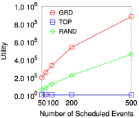
(a) Utility vs. $k$

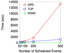
(b) Time vs. $k$

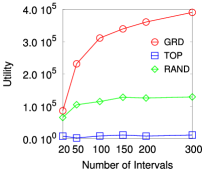
(c) Utility vs. $|\mathcal{T}|$

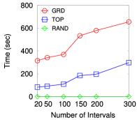
(d) Time vs. $|\mathcal{T}|$

Figure 1: Varying the number of: (1) scheduled events $k$; and (2) time intervals $|\mathcal{T}|$

Parameters. Adopting the same setting as in the related works [6, 11, 12, 13, 15], we set the the default and maximum value of the of scheduled events $k$, to $100$ and $500$, respectively. Also, we vary the number of time intervals $|\mathcal{T}|$, from $\frac{k}{5}$ up to $3k$, with default value set to $\frac{3k}{2}$. Further, the number of candidate events $|\mathcal{E}|$ is set to $2k$.

In order to select the values for the number of competing events per interval, we analyze the two Meetup datasets from [9]. From the analysis, we found that, on average, $8.1$ events are taking place during overlapping intervals. Therefore, the number of competing events per interval is selected by a uniform distribution having $8.1$ as mean value.

Regarding the value for the number of available events’ locations, we consider the percentage of pairs of events that are spatio-temporally conflicting, as specified in [11]. As a result, we set the number of available locations to $25$. The social activity probability $\sigma_{u}^{t}$ is defined using a Uniform distribution.

The performance and the effectiveness of the examined methods are marginally affected by the available/required resources parameters (here as resources we consider organizer’s staff). Hence, we choose a reasonable number based on our scenario, setting the number of available resources to $20$. Also, the number of required resources is selected by a uniform distribution defined over the interval $[1,\frac{20}{3}]$.

Methods. In our evaluation we study our method GRD, as well as two baselines. The first baseline method, TOP, computes the assignment scores for all the events and selects the events with $top$-$k$ score values. The second, denoted as RAND assigns events to intervals, randomly. Note that, since the objective, the solution and the setting of our problem are substantially different (see Sect. I) from the related works [6, 12, 13, 11, 15, 14, 5, 2], the existing methods cannot be used to solve the SES problem. All algorithms were written in C++ and the experiments were performed on an 2.67GHz Intel Xeon E5640 with 32GB of RAM.

IV-B Results

In the first experiment, we study the effect of varying the number of scheduled events $k$. In terms of utility (Fig. 1a), we observe that, in all cases, GRD outperforms significantly both baselines. The difference between RAND and GRD increases as $k$ increases. This is expected considering the fact that the larger the $k$, the larger the number of “better”, compared to random, selected assignments. Finally, TOP reports considerably low utility scores in all cases.

The results regarding the execution time are depicted in Figure 1b. Note that the computations that are performed due to updates increase with $k$, while the number of initially computed scores is the same for all $k$. Also, TOP performs only the initial scores’ computations (there are no score updates). That’s why the difference between the GRD and the TOP increases with $k$.

In the next experiment, we vary the number of time intervals $|\mathcal{T}|$. Regarding utility (Fig. 1c), we observe that, as the number of intervals increases, the utility of GRD and TOP methods increases too. This happens because the increase of available intervals results to a smaller number of events assigned in the same interval, as well as to a larger number of candidate assignments. In terms of execution time (Fig. 1d), for the same reason as in the first experiment, the difference between the GRD and the TOP increases with $|\mathcal{T}|$.

V Conclusions

This paper introduced the Social Event Scheduling (SES) problem. The goal of SES is to maximize the overall events’ attendance considering several events’ and users’ factors. We showed that SES is strongly NP-hard and we developed a greedy algorithm.

References

- [1] I. Boutsis, S. Karanikolaou, and V. Kalogeraki. Personalized event recommendations using social networks. In MDM, 2015.
- [2] Y. Cheng, Y. Yuan, L. Chen, C. G. Giraud-Carrier, G. Wang. Complex event-participant planning and its incremental variant. In ICDE, 2017.
- [3] R. Du, Z. Yu, T. Mei, Z. Wang, Z. Wang, and B. Guo. Predicting Activity Attendance in Event-based Social Networks: Content, Context and Social Influence. In UbiComp, 2014.
- [4] K. Feng, G. Cong, S. S. Bhowmick, and S. Ma. In Search of Influential Event Organizers in Online Social Networks. In SIGMOD, 2014.
- [5] J. Huang, Y. Zhou, X. Jia, and H. Sun. A novel social event organization approach for diverse user choices. The Computer Journal, 2016.
- [6] K. Li, W. Lu, S. Bhagat, L. V. Lakshmanan, and C. Yu. On Social Event Organization. In KDD, 2014.
- [7] X. Liu, Q. He, Y. Tian, W. Lee, J. McPherson, J. Han. Event-based social networks: linking the online and offline social worlds. KDD 2012
- [8] S. Martello and P. Toth. Knapsack Problems: Algorithms and Computer Implementations. John Wiley & Sons, 1990.
- [9] T. N. Pham, X. Li, G. Cong, Z. Zhang. A General Graph-based Model for Recommendation in Event-based Social Networks. In ICDE, 2015.
- [10] D. Romero, K. Reinecke, L. Robert. The influence of early respondents: information cascade effects in online event scheduling. WSDM 2017
- [11] J. She, Y. Tong, and L. Chen. Utility-Aware Social Event-Participant Planning. In SIGMOD, 2015.
- [12] J. She, Y. Tong, L. Chen, and C. C. Cao. Conflict-aware Event-participant Arrangement. In ICDE, 2015.
- [13] J. She, Y. Tong, L. Chen, and C. C. Cao. Conflict-aware Event-participant Arrangement and Its Variant for Online Setting. TKDE, 2016.
- [14] J. She, Y. Tong, L. Chen, and T. Song. Feedback-Aware Social Event-Participant Arrangement. In SIGMOD, 2017.
- [15] Y. Tong, J. She, and R. Meng. Bottleneck-aware Arrangement Over Event-based Social Networks: The Max-Min Approach. WWWJ, 2015.
- [16] T.Xu, H.Zhong, H Zhu, H Xiong, E Chen, G Liu. Exploring the impact of dynamic mutual influence on social event participation. In SDM 2015
- [17] W. Zhang, J. Wang, W. Feng. Combining Latent Factor Model with Location Features for Event-based Group Recommendation. KDD, 2013.
- [18] X. Zhang, J. Zhao, and G. Cao. Who Will Attend? - Predicting Event Attendance in Event-based Social Network. In MDM, 2015.