Diffusion with Resetting Inside a Circle

Abstract

We study the Brownian motion of a particle in a bounded circular 2-dimensional domain, in search for a stationary target on the boundary of the domain. The process switches between two modes: one where it performs a two-dimensional diffusion inside the circle and one where it travels along the one-dimensional boundary. During the diffusion, the Brownian particle resets to its initial position with a constant rate $r$. The Fokker-Planck formalism allows us to calculate the mean time to absorption (MTA) as well as the optimal resetting rate for which the MTA is minimized. From the derived analytical results the parameter regions where resetting reduces the search time can be specified. We also provide a numerical method for the verification of our results.

I Introduction

A large range of phenomena are characterized by the properties of first passage time of different stochastic processes Redner01 . A special case of them are related to search processes that take place in confinement and have long been an object of scientific research Querin . They find applications among a large range of distinct fields such as microbiological systems, network theory and computer science Redner14 ; Gelenbe ; Montanari . In the last few years, the mean time to absorption (MTA) for many target processes inside different bounded domains have been evaluated. For most stochastic processes, an analytical expression in an arbitrary domain is rather difficult to establish Benichou05 . Nevertheless progress can be made by the study of general concepts like the reduction of dimensionality Holyst ; Benichou09 ; Benichou07 ; Evans12dec in well defined domains. Here we consider such a simple confining geometry inside of which a stochastic search process combining two-dimensional diffusion inside a circle with one-dimensional diffusion on the periodic boundary takes place. We ask ourselves how the implementation of a resetting mechanism, which forces the diffusive searcher to return to its initial position, will influence the MTA if we assume that the target on the boundary is perfectly absorbing.

A resetting mechanism like the one introduced in the previous paragraph may seem purely artificial but it is strongly inspired by patterns often encountered in nature. For example animals may relocate to previously visited positions in order to improve their searching strategy Boyer . Stochastic processes performing resetting as well as effectively reducing their dimensionality find apllications in various systems. For macrobiological processes like foraging catalan such a combination arises naturally, for instance, hunting along the shore of a lake and returning to the roost. At the same time reduction of dimensionality can be considered as fulfillment of a constraint in terms of a randomized search algorithm which in general profit from a restart mechanism Pal17 .

Our study builds on an increasing amount of works discussing stochastic processes with resetting Shkilev ; Kusmierz2 ; Sharma which became only recently a subject of study in the physics literature Zanette ; Montero13 . The interest on this field was strongly boosted by the work of Evans and Majumdar who first analyzed the case of a one-dimensional Brownian motion modified by a resetting mechanism Evans11 . The search properties of this process have been studied by considering an absorbing target at the origin and calculating the mean first passage time $T$ to the origin as a function of the resetting rate $r$. It is clear that $T$ diverges as $T\sim r^{-1/2}$ for $r\rightarrow 0$, which recovers the well-known result that the mean first passage time for a purely diffusive particle is infinite. Also as $r\rightarrow\infty$, the particle hardly gets an opportunity to diffuse away from its starting position and remains localized for an indefinite time. As a result, $T$ diverges. It is evident that a minimum exists for $T$ since $T$ diverges in the two limits $r\rightarrow 0$ and $r\rightarrow\infty$.

This setting has shown the drastic effect of a resetting mechanism on the distribution of search times and has lead to several questions with regard to the dynamics of similar processes. So the generalization of this problem for the special cases of space-depending rates, resetting to a random position with a given distribution and to a spatial distribution of the target were presented in Evans112 . It has also been shown that the presented formalism can easily be expanded for the higher dimensional cases Evans14 . At the same time the properties of the non-equilibrium steady state have been evaluated for the special case of a diffusion inside a potential landscape APal .

Next to the archetype of diffusion processes with resetting several other stochastic processes have been analyzed in a resetting context. As an example, for the first order transition observed for a Levy flight process with resetting, the mean first passage time and the optimal search time have been evaluated in Kusmierz . This very interesting property of phase transitions was treated extensive in Campos ; Touchette while even the thermodynamics of this process could be analyzed Fuchs . Furthermore resetting is not only relevant for stochastic search processes as the work of Gupta et. al. Gupta ; Gupta2 shows, where the effect of a persistent resetting mechanism on the time evolution of fluctuating surfaces has been studied.

In the recent past the important influence of memory in the foraging behavior of macrobiological organisms was analyzed by Boyer et al. in Boyer17 where the properties of a stochastic process resetting to a previously visited site has been evaluated. Next to the evaluation of the resetting rate in the last years the optimal resetting time distribution could also been determined Apal2 . Lastly we have to note that in most of the presented models the resetting mechanism could be considered as an external mechanism. A variation of this property was presented in the work of Falcao and Evans Falcao , where the possibility of a resetting relies on the internal dynamics.

In the following we imagine that we have a stochastic searcher starting from a position inside of a circle with radius $R$. At the same time we have a stationary target on the boundary of the circle. The stochastic searcher performs a two-dimensional Brownian motion with the diffusion constant $D_{2}$ until it arrives at the boundary of the circle. The searcher then sticks to the boundary and undergoes a one-dimensional diffusion with diffusion constant $D_{1}$ along the boundary. With a constant rate $r$ the particle then resets to the initial position inside the circle. Then again the particle performs a two-dimensional diffusion until it arrives at the boundary and so on. The process terminates when the searcher finds the target. We assume here that the target has no dimension which ensures that such a termination is possible only during the one-dimensional diffusion phase. This assumption allows to calculate the MTA exactly by using the results derived in a large number of works on stochastic processes with resetting in the last few years.

This paper is structured as follows: we will first remind the readers about the properties of diffusion processes with stochastic resetting. In Sec. II we will hereto consider the case where the initial position of the particle is on the boundary of the circle and analyze the corresponding MTA. In Sec. III we focus on the case with an initial position at the center of the circle and compare our results to previous works in an intermittent setting Moreau11 . In Sec. IV we analyze the properties for general initial conditions. We will first derive an expression for the gain potential. This provides the master equation of the process which can then be solved in order to give us the desired MTA. Furthermore, we will characterize the different areas for which a resetting proves beneficial, depending on the parameters $D_{2}$, $D_{1}$ and $r$. In Sec. V we will follow the same approach as in Sec. IV in order to analyze the properties of the generalized process where resetting may even occur during the two-dimensional diffusion. In the last section we will focus on open questions and possible extensions of the present work.

II Diffusion with Resetting in one-dimensional periodic domain

We start with the simpler problem of an initial position on the boundary of the circle. In this case we do not need to consider the two-dimensional diffusion as this case boils down to just a one-dimensional diffusion process with resetting in a periodic domain of length $L=2\pi R$.

Let us first recapitulate some basic properties of the one-dimensional diffusion with resetting. In order to fully describe a resetting process by a Fokker-Planck equation formalism we need to define different potentials describing the dynamics of the resetting process. One needs to define a resetting potential $\mathcal{P}_{S}(x)$ responsible for the particle removal associated to the relocation of the particles. This potential is in turn complemented by the gain potential $\mathcal{P}_{G}(x)$, which is responsible for the reappearance of the particles at a different position derived from the corresponding distribution function. Finally, as we are dealing with a target process, we need to insert an annihilation potential $\mathcal{P}_{A}(x)$.

This allows us to describe the evolution of the probability density function $\psi(x,t;x_{0})$ for a process starting from the position $x_{0}$ at the time-point $t=0$, by solving the master equation

$$\frac{\partial\psi(x,t;x_{0})}{\partial t}=D\frac{\partial^{2}\psi(x,t;x_{0})}{\partial x^{2}}+\mathcal{P}_{G}(x)\int\,\mathrm{d}x^{\prime}\,\mathcal{P}_{S}(x^{\prime})\psi(x^{\prime},t;x_{0})-\mathcal{P}_{S}(x)\psi(x,t;x_{0})-\mathcal{P}_{A}(x)\psi(x,t;x_{0}).$$ (1)

This Fokker-Planck equation above can be generally used in order to describe the dynamics for a large range of search processes. The insertion of the potential $\mathcal{P}_{A}$ allows us to study even processes with partial absorbing conditions Sano ; Whitehouse ; Scha . Since in the presented problems perfect absorbing boundary conditions are implied, the annihilation potential $\mathcal{P}_{A}$ can be replaced by the boundary conditions

$$\psi(0,t;x_{0})=\psi\left(L,t;x_{0}\right)=0.$$ (2)

From the Fokker-Planck equation one can easily derive the backward master equation fulfilled by the survival probability $Q(x_{0},t)$,

$$Q(x_{0},t)=\int\,\mathrm{d}x\,\psi(x,t;x_{0})$$ (3)

describing the probability for a process to have survived up to the time-point $t$ if it started from the position $x_{0}$. It is indeed possible to derive $Q(x_{0},t)$ for a large range of potentials describing complex dynamics, as we shall encounter in Sec. IV.

The first process which we deal with is the one-dimensional process returning to its initial position after each reset with a uniform resetting field and two perfect absorbing boundaries. In order to solve this problem we are assuming now that $x_{r}$ is the position of the particle after the reset. So we set $\mathcal{P}_{G}(x)=\delta(x-x_{r})$ and $\mathcal{P}_{S}(x)=r$ with $\psi(0,x_{0};t)=\psi(L,x_{0};t)=0$.

It is not hard to see that in this case the backward master equation (1) can be replaced by following expression

$$\frac{\partial Q(x,t)}{\partial t}=D_{1}\frac{\partial^{2}Q(x,t)}{\partial x^{2}}-rQ(x,t)+rQ(x_{0},t)$$ (4)

with

$$Q(0,t)=Q(L,t)=0.$$ (5)

In order to solve this differential equation we can use the Laplace-Transform

$$\tilde{q}(x,s)=\int\limits_{0}^{\infty}\,\mathrm{d}t\,Q(x,t)e^{-st}$$ (6)

leading to

$$D_{1}\frac{\partial^{2}\tilde{q}(x,s)}{\partial x^{2}}-(r+s)\tilde{q}(x,s)+1+r\tilde{q}(x_{r},s)=0.$$ (7)

which yields Evans14

$$\tilde{q}(x,s)=Ae^{\sqrt{\frac{r+s}{D_{1}}}x}+Be^{-\sqrt{\frac{r+s}{D_{1}}}x}+\frac{1+r\tilde{q}(x_{r},s)}{r}.$$ (8)

Now by setting $s=0$ we are in the position to calculate the mean time to absorption

$$T(x)=-\int_{0}^{\infty}\,\mathrm{d}t\,t\frac{\partial Q(x,t)}{\partial t}=\tilde{q}(x,0)$$ (9)

for which the expression

$$T(x)=Ae^{\ell^{-1}x}+Be^{-\ell^{-1}x}+\frac{1+rT(x_{r})}{r}$$ (10)

with $T(0)=T(L)=0$ holds. We used hereby the notation

$$\ell=\sqrt{\frac{D_{1}}{r}}$$ (11)

for the mean free path length between two resets.

We now can make the assumption that

$$\frac{\partial}{\partial x}T(x)|_{x=L/2}=0$$ (12)

which together with the two boundary conditions leads to the solution

$$T(x)=\frac{1+rT(x_{r})}{r}\left(1-\frac{\cosh\ell^{-1}(x-L/2)}{\cosh\ell^{-1}L/2}\right)$$ (13)

For the special case of $x_{r}=x$, namely the case where the particle resets to its initial position, we can derive the formula

$$T(x)=-\frac{\ell^{2}}{D_{1}}\left(1-\frac{\sinh\ell^{-1}L}{\sinh\ell^{-1}x+\sinh\ell^{-1}(L-x)}\right).$$ (14)

This result allows us to address the question with regard to the dependence of the mean time on the starting position.

We define therefore the optimal free path length, $\ell^{*}$, as the value of $\ell$ for which

$$\frac{\partial}{\partial\ell}T(x)|_{\ell=\ell^{*}}=0$$ (15)

holds. In Fig. 1 we can see that by decreasing the distance between the starting position and one of the boundaries a crossover for the optimal mean free path length from an infinite value to a finite one takes place. This is particularly interesting from a physical point of view. For initial positions near the boundaries, a finite traveling distance between two resets and hence $r>0$ is efficient. As soon as the particle starts at a position between the crossover points $(0.276L,0.724L)$, an infinite time interval between resets and thus pure diffusive motion is preferred.

Figure 1: Inverse of the optimal mean free path length vs the starting position of the searcher for a system of length $L=1$. We can see that for $0.276L<x_{0}<0.724L$ the optimal mean free path length is equal to $\infty$. This fact changes if we consider a starting position which is closer to the boundaries and thus a finite value for the mean free path length tends to be optimal.

III Hard Resetting

Let us now consider the case where the initial position is at the center of the circle. We will characterize this process from now on as hard reset process. It can be treated as a special case of the general process presented in the next section. We treat this special case here first since the presented results confirm previous discoveries which were derived for processes that exhibit intermittent dynamics Benichou10 ; Benicou14 . Furthermore this first problem is actually rather simple and thus a good introduction to our general approach.

Since the particle finds itself in the center of the circle after each reset the subsequent one-dimensional excursion will start from an arbitrary point on the circle due to the radial symmetry. This allows us to use the uniform probability distribution function $\mathcal{P}_{G}(x)=L^{-1}=\left(2\pi R\right)^{-1}$ $\forall x\in[0,2\pi R]$ for the gain potential in equation (1).

In order to calculate the MTA we will have to calculate the mean time for each of the two different modes consisting purely of one- and two-dimensional diffusion. Let $T_{1}$ be the mean time the particle spends during its one-dimensional diffusion and $T_{2}$ the mean time for the two-dimensional path then the total mean time to absorption is given by,

$$T=T_{1}+T_{2}.$$ (16)

For this simple process the MTA is given by

$$T=rT_{1}\tau_{2}+T_{1}+\tau_{2},$$ (17)

where $\tau_{2}$ is the mean time that a Brownian particle starting at the center of a circle with radius $R$ needs in order to reach the boundary (mean time to boundary, MTB). This quantity is easily derived from the expression Redner01

$$\tau_{2}(R)=\frac{R^{2}}{4D_{2}}.$$ (18)

In order to determine the MTA of the one-dimensional diffusion we just need to find the solution to the differential equation

$$-1=D_{1}\frac{\partial^{2}}{\partial x^{2}}T_{1}(x)-\frac{r}{L}T_{1}(x)+\frac{r}{L}\int\,\mathrm{d}z\,T(z)$$ (19)

with the boundary conditions

$$T(0)=T(L)=0.$$ (20)

Which as shown in the previous section takes the form

$$T(x)=-A\frac{\cosh\ell^{-1}(x-L/2)}{r\cosh L\left(2\ell\right)^{-1}}+\frac{L}{r}+F(0,L).$$ (21)

where we used the notation $F(0,L)=\int_{0}^{L}\,\mathrm{d}z\,T(z)$. From the boundary conditions we can determine the constant $A$ as,

$$A=rF(0,L)+L.$$ (22)

Reinserting the above expression in the general form described in (21) and evaluating $F(0,L)$ gives us

$$F(0,L)=\left(\frac{L}{r}+F(0,L)\right)\left(1-2\ell\tanh L\left(2\ell\right)^{-1}\right)$$

from which we obtain

$$F(0,L)=\frac{L}{r}\left(\left(2\ell\right)^{-1}\coth L\left(2\ell\right)^{-1}-1\right)\,.$$ (23)

Finally we have

$$T(x)=\frac{L\coth L\left(2\ell\right)^{-1}}{2\ell r}\left(1-\frac{\cosh\ell^{-1}(x-L/2)}{\cosh L\left(2\ell\right)^{-1}}\right).$$ (24)

Figure 2: Numerical evaluation of the formula (24) for $x_{0}=0.5$ with $L=1$. We have chosen here, as before, $D_{1}=5\cdot 10^{-7}$.

From (24) one can see that the mean time to absorption is minimized for $\ell\rightarrow 0$. In order to prove this result we use the following variation of the original problem. We consider the gain potential

$$\mathcal{P}_{G}(x)=\begin{cases}\frac{1}{1-2\varepsilon}&\quad\text{if }\varepsilon<x<1-\varepsilon\\ 0&\quad\text{else }\\ \end{cases}$$ (25)

which restores the original uniform potential in the limit $\varepsilon\rightarrow 0$. For the potential described by equation (25) and $L=1$ we get the mean time

$$T(x)=\frac{(1-2\varepsilon)\left(\cosh\left(2\ell\right)^{-1}-\cosh\ell^{-1}(x-1/2)\right)}{2r\ell\sinh\ell^{-1}(1/2-\varepsilon)}.$$ (26)

For small values of $\ell$ and $x\in[0,1]$ we have

$$\left(1-\frac{\cosh\ell^{-1}(x-1/2)}{\cosh\left(2\ell\right)^{-1}}\right)\simeq 1.$$ (27)

This allows us to replace equation (26) above with the expression

$$T(x)=\frac{\sigma^{-2}2(1-2\varepsilon)\ell}{\tanh\left(2\ell\right)^{-1}-\cosh\ell^{-1}\varepsilon-\sinh\ell^{-1}\varepsilon}.$$

Now by using

$$\tanh\left(\frac{\ell^{-1}}{2}\right)\simeq 1,$$ (28)

for small values of $\varepsilon$ we can simplify our formula to

$$T(x)=\varepsilon\sigma^{-2}(1-2\varepsilon)\frac{e^{\ell^{-1}\varepsilon}}{\ell^{-1}\varepsilon}.$$ (29)

We also see that for high values of the resetting rate, the mean time becomes independent of the initial position since due to the resetting, the information with regard to the initial position gets lost for increasing times.

Now we need to consider that the function $x^{-1}e^{x}$ has a minimum for $x=1$. Correspondingly, the optimal resetting rate for this one-dimensional problem is achieved when $\ell^{-1}=\varepsilon^{-1}$. By sending now $\varepsilon$ to zero, in order to regain the original problem, we notice that the optimal resetting rate goes to infinity.

Figure 3: MTA for the hard resetting problem in the special case of $D_{2}/D_{1}=2$ for $R=(2\pi)^{-1}$ and $D_{1}=5\cdot 10^{-7}$.

Figure 4: MTA for the hard resetting problem in the special case of $D_{2}/D_{1}=0.25$ for $R=(2\pi)^{-1}$ and $D_{1}=5\cdot 10^{-7}$.

Although there is no finite optimal resetting rate for the one-dimensional case, the situation changes when we consider the two-dimensional excursion of the particle. We evaluate therefore Eq. (17) by implementing Eq. (18) and Eq. (24) and integrating over the interval $[0,L]$ leading to

$$T=\frac{R^{2}}{4D_{2}}+\frac{\left(L\coth L\left(2\ell\right)^{-1}-2\ell\right)}{2r\ell}\left(\frac{rR^{2}}{4D_{2}}+1\right).$$ (30)

This expression is in perfect agreement with Eq. (2.23) of Benicou14 . By using the series expansion of the cotangent function we rewrite this expression as

$$T=\frac{R^{2}}{4D_{2}}+\frac{2}{D_{1}}\left(1+\frac{r}{D_{2}}\right)\sum\limits_{k=0}^{\infty}\frac{L^{-1}}{\left(\frac{2\pi k}{L}\right)^{2}+\frac{r}{D_{1}}}.$$ (31)

It follows from this result that an optimal resetting rate can be found only if $D_{2}/D_{1}\geq 0.38$. This result is easily obtained by a numerical evaluation of the formula above. In Figs. 3 and 4 we can see the diverse behavior of the mean time to absorption for different values of $\ell$ for values above and below the critical value of $D_{2}=0.38D_{1}$ respectively.

IV Partial Resetting

Now we consider the general case where the initial position lies inside the circle and is not the center. We start with the problem where resetting can only take place from the boundary of the domain. We will characterize this strategy from now on as partial reset process. In the next section we will consider the problem of a persistent resetting field, where resetting can take place from anywhere during the Brownian motion of the particle, including from aywhere inside the circle, irrespective of whether the particle is undergoing one-dimensional or two-dimensional diffusion.

Let us first imagine that our particle starts from the position, given by the polar coordinates $\vec{x}=\left(R_{0},\theta_{0}\right)$, where $R_{0}$ is the distance from the center and $\theta_{0}$ is the angle it makes with the vertical. After a two-dimensional excursion the particle arrives at the circle. The mean time for this arrival at the boundary is given by

$$\tau_{2}(R,R_{0})=\frac{R^{2}-R_{0}^{2}}{4D_{2}}.$$ (32)

Depending on the parameters $R_{0}$ and $\theta_{0}$ the likelihood of crossing the boundary at a specific angle has to be calculated. This allows us to determine the probability distribution function of the starting position for the subsequent one-dimensional diffusion phase. In order to compute the probability distribution function of the hitting angle we can use an electrostatics analogy Redner01 which leads to

$$\mathcal{P}(\theta;\theta_{0},R_{0})=\frac{1-\frac{R_{0}^{2}}{R^{2}}}{2\pi R\Big{(}1-\frac{2R_{0}\cos(\theta-\theta_{0})}{R}+\frac{R_{0}^{2}}{R^{2}}\Big{)}}.$$ (33)

Figure 5: Mean time to absorption for a Brownian process starting inside a two-dimensional circle for different initial conditions $(R_{0},\theta)$. The points were determined by a Monte-Carlo simulation with $D_{2}=10^{-6}$, $2D_{1}=D_{2}$ and $R=1/2\pi$. The lines correspond to our theoretical values for these parameters.

Let $x_{0}$ be the point on the boundary of the circle that lies on the line connecting the initial position $\vec{R}_{0}=\left(\theta_{0},R_{0}\right)$ to the center of the circle and is closest to the initial position. Then $\mathcal{P}_{G}(z)=\mathcal{P}(\theta,R_{0})$ holds, if we assume that $R(\theta-\theta_{0})=(z-x_{0})$. Inserting this expression in Eq. (1) we can get following backward equation for the mean time to absorption for a process starting on the boundary at the position $x$,

$$0=D_{1}\frac{\partial^{2}}{\partial x^{2}}T(x)-rT(x)+1+r\int\,\mathrm{d}z\,P_{G}(z)T(z).$$ (34)

Using the boundary condition $T(0)=T(2\pi R)=0$ together with Eq. (12) we can easily solve this non-homogeneous differential equation of second order to deliver

$$T(x)=\left(\frac{1}{r}+\int\,\mathrm{d}z\,\mathcal{P}_{G}(z)T(z)\right)\left(1-\frac{\cosh\ell^{-1}(x-\pi R)}{\cosh\ell^{-1}\pi R}\right).$$ (35)

If we multiply now both sides of this formula with $\mathcal{P}_{G}(x)$ and integrate over the interval $[0,2\pi R]$ we can see that

$$T(x)=\frac{\cosh\sqrt{\frac{r}{D}}\frac{L}{2}-\cosh\sqrt{\frac{r}{D}}\left(x-L/2\right)}{r\int\,\mathrm{d}z\,\mathcal{P}_{G}(z)\cosh\sqrt{\frac{r}{D}}\left(z-L/2\right)}$$ (36)

holds.

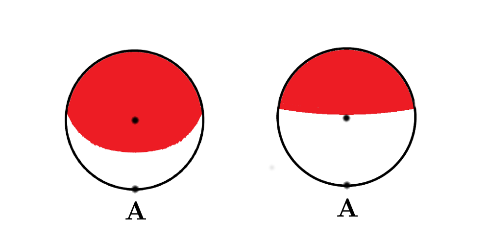
Figure 6: Different regimes with regard to the existence of an optimal resetting rate for different initial position for a Brownian particle in search for a target located at A. The left figure corresponds to the choice of parameters with $D_{2}/D_{1}=0.25$ and on the right to $D_{2}=D_{1}$. The shaded area (red) describes initial positions for which no positive optimal resetting rate can be found. We can see that for $D_{2}/D_{1}=1$ a particle starting from the center of the circle can be optimized through a positive resetting rate.

The MTA is thus given by the expression

$$T_{1}=\int\,\mathrm{d}z\,\mathcal{P}_{G}(z)T(z).$$ (37)

Implementing all of these results in Eq. (17) we get

$$T=\frac{R^{2}-R_{0}^{2}}{4D_{2}}+\left(\frac{1}{r}+\frac{R^{2}-R_{0}^{2}}{4D_{2}}\right)\times$$

$$\times\int\,\mathrm{d}x\,\mathcal{P}_{G}(x)\frac{\cosh\sqrt{\frac{r}{D_{1}}}\pi R-\cosh\sqrt{\frac{r}{D_{1}}}\left(x-\pi R\right)}{\int\,\mathrm{d}z\,\mathcal{P}_{G}(z)\cosh\sqrt{\frac{r}{D_{1}}}\left(z-\pi R\right)}.$$ (38)

In Fig. 5 we can observe a very good agreement between this formula and the results of Monte-Carlo simulations.

The derived equation gives us the opportunity to characterize the different regimes inside the circle for which an optimal resetting rate can be found. In Fig. 6 we represent the respective areas for the ratios of $D_{2}=0.25D_{1}$ and $D_{2}=D_{1}$ which are below and above the characteristic value of $D_{2}=0.38D_{1}$, that was determined in the last section. In both figures the $R_{0}/R=1$ axis is crossed at the value of $\theta=0.56\pi$, which is in perfect agreement with the results of Sec. II.

V Persistent Resetting

In the previous section we could determine for specific values of the ratio $D_{2}/D_{1}$ the different regimes for which a resetting from the boundary could be beneficial. In this section we analyze the dynamics for a process for which resetting takes place not only from the boundary, but also from inside of the circle. We consider also a permanent resetting field and characterize in the following the process as persistent reset process.

While the formalism and approach of the previous sections proves useful, special care with regard to two characteristics of the present problem have to be taken into account. The first is the modification of the MTB, $\tau_{2}$, due to the resetting mechanism. The second is the effect of the resetting mechanism on the hitting angle distribution.

We start with the first point, the goal being to determine the conditions under which an optimal resetting rate with regard to $\tau_{2}$ can be found. Let $\vec{x}_{r}$ be the position of resetting then the two-dimensional excursions of the particle are described by the backward equation

$$D_{2}\nabla^{2}\tilde{q}(\vec{x},s)-(r+s)\tilde{q}(\vec{x},s)=-1-r\tilde{q}(\vec{x}_{r},s)$$ (39)

with the boundary condition

$$\tilde{q}\left(\vec{x},s\right)|_{|\vec{x}|=R}=0.$$ (40)

We start by providing the solution to the homogeneous equation

$$D_{2}\nabla^{2}\tilde{q}(\vec{x},s)-(r+s)\tilde{q}(\vec{x},s)=0$$ (41)

which is radially symmetric about the origin and has a vanishing derivative at $|\vec{x}|=0$

$$\nabla\tilde{q}(\vec{x},s)|_{\vec{x}=\vec{0}}=0.$$ (42)

These conditions are fulfilled by the equation

$$\tilde{q}_{hom}(\vec{x},s)=I_{0}\left(\sqrt{\frac{r+s}{D_{2}}}|\vec{x}|\right)$$ (43)

where $I_{n}$ is the modified Bessel function of the first type.

Now we can use this expression in order to solve the differential equation (39), by considering, as before, the Ansatz

$$\tilde{q}\left(\vec{x},s\right)=AI_{0}\left(\sqrt{\frac{r+s}{D_{2}}}|\vec{x}|\right)+B.$$ (44)

By taking into account the boundary condition we can derive the solution

$$\tilde{q}\left(\vec{x},s\right)=\frac{I_{0}\left(\ell^{-1}_{s}R\right)-I_{0}\left(\ell^{-1}_{s}|\vec{x}|\right)}{rI_{0}\left(\ell^{-1}_{s}|\vec{x}_{r}|\right)+sI_{0}\left(\ell^{-1}_{s}R\right)}$$ (45)

with $\ell^{-1}_{s}=\sqrt{(r+s)/D_{2}}$. For the problems studied in this paper, where the resetting position $\vec{x}_{r}$ is equal to the starting position, we have

$$\tilde{q}\left(\vec{x},s\right)=\frac{I_{0}\left(\ell^{-1}_{s}R\right)-I_{0}\left(\ell^{-1}_{s}|\vec{x}|\right)}{rI_{0}\left(\ell^{-1}_{s}|\vec{x}|\right)+sI_{0}\left(\ell^{-1}_{s}R\right)}.$$ (46)

Now we can determine the MTB for this process provided by the formula

$$\tau_{2}(R_{0})=\tilde{q}\left(R_{0},s=0\right)=\frac{1}{r}\left(\frac{I_{0}\left(\ell^{-1}_{2}R\right)}{I_{0}\left(\ell^{-1}_{2}R_{0}\right)}-1\right)$$ (47)

with $\ell_{2}=\sqrt{D_{2}/r}$. In Fig, 7 we can see a very good agreement between the derived analytical solution and the Monte-Carlo simulation. Furthermore in Fig. 8 we determine the optimal resetting rate for a large range of values of the ratio $R_{0}/R$. As we can see, an optimal resetting rate can be found only for $R_{0}>0.578R$.

Figure 7: MTB for two-dimensional Brownian motion in a circle of radius $R=1$ starting from the radius $R_{0}=0.9$ for different inverse mean path lengths. We can clearly see that there exists an optimal resetting rate for which this time is minimized.

Figure 8: Inverse of the optimal mean free path length for different ratios of the initial radius to the total radius of the circle. We can see that for $R_{0}>0.578R$ the optimal resetting rate is greater than zero. We have used here a circle of radius $R=(2\pi)^{-1}$.

We can even calculate the ratio $D_{2}/D_{1}$ for which the effect of resetting is beneficial when starting from the center of the circle. We can use the same formula as before to show that the mean time to absorption in this case is given by

$$T=\frac{1}{r}\left(\frac{I_{0}\left(\ell^{-1}_{2}R\right)}{I_{0}\left(\ell^{-1}_{2}R_{0}\right)}-1\right)+\frac{I_{0}\left(\ell^{-1}_{2}R\right)}{I_{0}\left(\ell^{-1}_{2}R_{0}\right)}\times$$

$$\times\frac{\coth L(2\ell_{1})^{-1}}{2r\ell_{1}}\left(L-2\ell_{1}\tanh L\left(2\ell_{1}\right)^{-1}\right)$$ (48)

with $\ell_{1}=\sqrt{D_{1}/r}$. By evaluating this formula we can see that a necessary condition for the existence of an optimal resetting rate is $D_{2}>0.4D_{1}$. As expected, this value is slightly larger than the value ($D_{2}>0.38D_{1}$) calculated in the last section for the special case where the resetting field acts only on the boundary of the system.

Now we focus on the effect of the resetting on the hitting angle. As discussed in Belan a resetting mechanism has a significant effect on the outcome of an absorption process. This can be understood by considering the stochastic paths of the particle influenced by resetting as the paths of a renewal process. The mean length of these paths is proportional to $r^{-1}$. Successfully approaching the boundary is only possible for the direct paths between initial position and boundary.

We use the method introduced in Belan in order to calculate the effect. Let $P(\theta,t)$ describe the probability density function of the absorption time for a path that crosses the boundary at the point corresponding to the angle $\theta$, then the probability for the same outcome with a positive resetting rate $r$ is given by

$$P_{r}(\theta)=\frac{\tilde{P}(\theta,r)}{\tilde{P}(r)},$$ (49)

where $\tilde{P}(\theta,r)$ and $\tilde{P}(r)$ denote the Laplace Transforms of $P(\theta,t)$ and $P(t)=\int\,\mathrm{d}\theta\,P(\theta,t)$ evaluated at $r$, respectively. In order to calculate the probability distribution functions $P(\theta,t)$, the image method proves cumbersome. We therefore suggest a Monte-Carlo simulation for the calculation of this probability distribution function.

The calculation of the Laplace Transform $\tilde{P}(r)$ is easier on the other side, since

$$\tilde{P}(r)=-\int\limits_{0}^{\infty}\,\mathrm{d}t\,\frac{\partial Q(R_{0},t)}{\partial t}e^{-rt}=$$

$$=-e^{-rt}Q(R_{0},t)|_{0}^{\infty}-r\int\limits_{0}^{\infty}\,\mathrm{d}t\,e^{-rt}Q(R_{0},t)=$$

$$=\frac{2I_{0}(\ell^{-1}_{2}R_{0})}{I_{0}(\ell^{-1}R)+I_{0}(\ell^{-1}_{2}R_{0})}.$$ (50)

As in Sec. IV we can use this formula in order to determine the probability distribution function of the starting point on the circle $\mathcal{P}_{G}(z)=P_{r}(\theta)$ by setting $R(\theta-\theta_{0})=(z-x_{0})$.

This way we can summarize all results of the present section in the following formula

$$T=\frac{1}{r}\left(\frac{I_{0}\left(\ell^{-1}_{2}R\right)}{I_{0}\left(\ell^{-1}_{2}R_{0}\right)}-1\right)+\frac{I_{0}\left(\ell^{-1}_{2}R\right)}{I_{0}\left(\ell^{-1}_{2}R_{0}\right)}\times$$

$$\times\int\,\mathrm{d}x\,\mathcal{P}_{G}(x)\frac{\cosh\ell^{-1}_{1}\pi R-\cosh\ell^{-1}_{1}\left(x-\pi R\right)}{\int\,\mathrm{d}z\,\mathcal{P}_{G}(z)\cosh\ell^{-1}_{1}\left(z-\pi R\right)}.$$ (51)

This expression is in good agreement with our previous results. For example it is not hard to see that in the limit $D_{2}\rightarrow\infty$ the present formula is equivalent to Eq. (38).

Figure 9: MTA for a particle starting from the center of the circle of radius $R=(2\pi)^{-1}$ for different inverse mean path lengths. We can clearly see that there exists an optimal resetting rate for which this time is minimized. The results of the Monte-Carlo simulation show a very good agreement to the analytical expectations derived from the formula (48).

VI conclusion

In this work we studied the dynamics of a diffusive searcher which combines two different behaviors. In one mode the searcher undergoes a two-dimensional diffusion and in the second mode a one-dimensional diffusion process along the boundary is performed. We also assumed that the evolution of the process is accompanied by restarts allowing the searcher to return to its initial position.

We started by a Fokker-Planck formalism and used the Laplace Transform to calculate the mean time to absorption for several variations of the process. This allowed us to get a better understanding of the properties of random search processes with restarts in two-dimensional bounded domains. In the past we could show that resetting can be beneficial for the case of an one-dimensional diffusion process in a bounded domain Scha . The work presented here allows us to claim that this statement holds also for a diffusion process inside a two-dimensional domain.

Specifically we could see that for the case of a one-dimensional process taking place in a periodic domain of length $L$ an optimal resetting rate exists as long as the distance between the initial position and the target is smaller than $0.276L$. In the next section we found that if the resetting distribution applies on the whole interval $[0,L]$, then the optimal resetting rate is equal to $\infty$.

These results were especially useful when analyzing the process switching from two-dimensional diffusion to one-dimensional excursion on the boundary where a resetting field applies. For this problem we could determine several regions for which an optimal resetting rate that was bigger than zero for different values of the ratio $D_{2}/D_{1}$ between the two diffusion constants. It was also possible to show that when the process starts from the center of the circle an optimal resetting rate can be found as long as $D_{2}>0.38D_{1}$. This is in perfect agreement with the past findings of similar works concerned with processes exhibiting intermittent behavior Benichou10 . In the last section we considered the possibility of a reset from also inside the circle and have shown that when starting from the center of the circle a resetting rate that is bigger than zero can only be preferential when $D_{2}>0.4D_{1}$.

Another generalization of the present formalism could consist in the replacement of the point-like target by an extended area on the boundary. The presented methods can easily be implemented to solve the problem of a Brownian particle trying to escape from a bounded domain through a small window while under the effect of a resetting potential. This can be considered as a variation of the narrow escape problem Voituriez . It would be interesting to see if a positive resetting rate can accelerate this process.

In several works in the past discussing diffusion with resetting, the case of many searchers has also been considered Evans11 ; Evans14 ; Whitehouse . We think that such a consideration would also be interesting in the present setting. One could go even further and implement an interaction mechanism between these searchers by adopting a single-file diffusion process on the boundary of the circle.

*

Appendix A Monte-Carlo simulation

Figure 10: Numerical and analytical evaluation of the targeting problem with no resetting. We calculate the mean time to absorption for a Brownian particle starting from $x_{0}=1/2$ with two absorbing boundary conditions $T(0)=T(1)=0$. We can see that a comparison between our analytical and numerical results is only possible for low values of $\sigma$.

In order to compare our analytical findings with numerical results we relied upon Monte-Carlo simulations. An easy way to simulate a Brownian-like motion consists hereby of observing the evolution of a discrete time random walk $x_{t}$ with $t\in\mathbb{N}$, defined by

$$x_{t}=x_{0}+\sum_{k=0}^{t}\xi_{k}$$ (52)

whereas the random variables $\xi_{k}$ are drawn from a normal distribution with mean $0$ and variance $\sigma^{2}$.

The mean variance of the random walk is given by the formula

$$\mathbb{E}\left[x_{t}^{2}-x_{0}^{2}\right]=\mathbb{E}\left[\sum\limits_{i=1}^{t}(x_{i}-x_{i-1})^{2}\right]=\sigma^{2}t.$$ (53)

By comparing this expression to the Green’s function we see that $\sigma^{2}=2D_{1}$. This relation between these two scales (analytical and numerical) allows us to directly compare our numerical results to the derived analytical expressions.

We have to note here that one has to be careful with regard to the choice of standard deviation, since higher values of volatility may lead to discrepancies between the two approaches since the nature of the continuum (analytical) and the discrete (numerical) time-step processes is fundamentally different. This is shown in Figure 10 where the expected time to absorption for a process with no resetting and two perfectly absorbing boundary conditions is plotted for both numerical and analytical methods.

In the latter sections IV and V the implementation and understanding of the dynamics of two-dimensional Brownian motions became necessary. In order to achieve that, we considered a two-dimensional random walk described by the equation

$$\vec{x}_{t}=\left(x_{0}+\sum_{k=0}^{t}\xi_{k}\right)\vec{e_{x}}+\left(y_{0}+\sum_{k=0}^{t}\xi_{k}\right)\vec{e_{y}},$$ (54)

whereas $\xi_{k}$ is a white noise process derived from the Gaussian distribution $\mathcal{N}(0,\sigma)$. For the presented two-dimensional process we have a standard deviation given by $2D_{2}=\sigma^{2}$. This allows us to determine numerically the stopping time

$$\tau_{2}=\inf\left\{t\in\mathbb{N}:x_{t}^{2}+y_{t}^{2}\geq R^{2}\right\}.$$ (55)

For two-dimensional systems the offset is extremely hard to reduce in comparison to the one-dimensional processes. Fortunately we can rely hereby on two methods: using processes with a smaller volatility and/or introduce a finer time-scale. The first method is non-optimal since it leads to an increase of the mean time to absorption and correspondingly to higher running times.

We decided therefore to use the second method. We considered hereby that each time step consists of $\delta^{-2}$ smaller steps during which jumps of length $\delta\xi$ are performed. It is easy to see that by sending $\delta$ to zero the desired Wiener process can be approximated, but even for $\delta>0$ this method leads to a great improvement of the derived results. For section IV we have chosen $\delta=0.25$ and for section V $\delta=0.1$.

In order to simulate the resetting mechanism we introduced the resetting probability $r_{n}\in[0,1]$. After each jump the walker is reset to a new position with a probability $r_{n}$ according to the gain distribution $\mathcal{P}_{G}$. The mean time between two resets $\tau_{r}$ for this process is consequently given by the formula

$$\tau_{r}=1+\sum_{k=0}^{\infty}kr_{n}(1-r_{n})^{k}=1+\frac{1-r_{n}}{r_{n}}=\frac{1}{r_{n}}.$$ (56)

In our analytical calculations we know that the times intervals between two resets have an exponential distribution

$$P(t)=re^{-rt}$$ (57)

for which then the mean time is given by $\tau_{r}=\frac{1}{r}$.

A comparison between our analytical findings and the Monte-Carlo approach is made possible by adjusting the two parameters, $r_{n}$ and $r$, so that these two time scales are equal.

- (1) S. Redner, A Guide to First-Passage Processes (Cambridge University Press, 2001).
- (2) T. Guérin, N. Levernier, O. Bénichou, and R. Voituriez, Nature 534, 356 (2016).
- (3) R. Metzler, G. Oshanin, and S. Redner, First-Passage Phenomena and their Apllications (World Scientific, Singapore, 2014) Vol 35.
- (4) E. Gelenbe Phys. Rev. E 82, 061112 (2010).
- (5) A. Montanari and R. Zecchina Phys Rev Lett. 88, 178701 (2002).
- (6) S. Condamin, O. Bénichou, and M. Moreau, Phys. Rev. Lett. 95, 260601 (2005).
- (7) R. Hołyst, M. Błaźejczyk, K. Burdzy, G. Góralski, L. Bocquet, Physica A: Stat. Mech. Appl. 277, 71 (2000).
- (8) O. Bénichou, Y. Kafri, M. Sheinman, and R. Voituriez, Phys. Rev. Lett. 103, 138102 (2009).
- (9) O. Bénichou, M. Moreau, P.-H. Suet, and R. Voituriez, J. Chem. Phys. 126, 234109 (2007).
- (10) M. R. Evans, S. N. Majumdar and K. Mallick, J. Phys. A: Math. Theor. 46, 185001 (2013).
- (11) D. Boyer and Solis-Salas, Phys. Rev. Lett. 112, 240601 (2014)
- (12) F. Bartumeus, and J. Catalan, J. Phys. A: Math. Theor. 42, 43 (2009).
- (13) A. Pal and S. Reuveni, Phys. Rev. Lett. 118, 030603 (2017).
- (14) V.P. Shkilev, Phys. Rev. E 96, 012126 (2017)
- (15) Ł . Kuśmierz, M. Bier and E. Gudowska-Nowak J. Phys. A: Math Theor. 50, 18 (2017).
- (16) A. Scacchi and A. Sharma, Molecular Physics 116, 460 (2017).
- (17) S. C. Manrubia, and D. H. Zanette, Phys. Rev. E 59, 4945 (1999).
- (18) M. Montero, and J. Villarroel, Phys. Rev. E 87, 012116 (2013).
- (19) M. R. Evans, and S. N. Majumdar, Phys. Rev. Lett. 106, 160601 (2011).
- (20) M. R. Evans, and S. N. Majumdar, J. Phys. A: Math. Theor. 44, 435001 (2011).
- (21) M. R. Evans, and S. N. Majumdar, J. Phys. A: Math. Theor. 47, 285001 (2014).
- (22) A. Pal Phys. Rev. E 91, 012113 (2014).
- (23) Ł. Kuśmierz, S. N. Majumdar, S. Sabhapandit, and G. Schehr, Phys. Rev. Lett. 113, 220602 (2014).
- (24) D. Campos and V Méndez, Phys. Rev. E 92, 062115 (2015).
- (25) R. J. Harris, and H. Touchette, J. Phys. A: Math. Theor. 50, 10LT01 (2017)
- (26) J. Fuchs, S Goldt, and U. Seifert, Europhys. Lett. 113, 60009 (2016).
- (27) S. Gupta, S. N. Majumdar, and G. Schehr, Phys. Rev. Lett. 112, 220601 (2014).
- (28) S. Gupta, and A. Nagar, J. Phys. A: Math Theor. 49, 445001 (2016).
- (29) D. Boyer, M. R. Evans, and S. N. Majumdar, J. Stat. Mech. 023208, 2017.
- (30) A. Pal, and S. Reuveni, Phys. Rev. Lett. 118, 030603 (2017).
- (31) R. Falcao and M. R. Evans, J. Stat. Mech. 17, 023204 (2017).
- (32) O. Bénichou, C. Loverdo, M. Moreau, and R. Voituriez, Rev. Mod. Phys. 83, 81 (2011).
- (33) H. Sano and M. Tachiya, J. Chem. Phys. 71, 1276 (1979).
- (34) J. Whitehouse, M. R. Evans and S. N. Majumdar, Phys. Rev. E 87, 022118 (2013).
- (35) C. Christou and A. Schadschneider, J. Phys. A: Math Theor. 48, 28 (2015)
- (36) O. Bénichou, D. Grebenkov, P. Levitz, C. Loverdo, and R. Voituriez, Phys. Rev. Lett. 105, 150606 (2010).
- (37) O. Bénichou, D. S. Grebenkov, L. Hillairet, L. Phun, R. Voituriez, and M. Zinsmeister, Analysis and Mathematical Physics 5, 321-362 (2015).
- (38) S. Belan, https://arxiv.org/pdf/1703.01486 (2017).
- (39) O. Bénichou and R. Voituriez, Phys. Rev. Lett. 100, 168105 (2008).