Observational constraints on quantum decoherence
during inflation

Abstract

Since inflationary perturbations must generically couple to all degrees of freedom present in the early Universe, it is more realistic to view these fluctuations as an open quantum system interacting with an environment. Then, on very general grounds, their evolution can be modelled with a Lindblad equation. This modified evolution leads to quantum decoherence of the system, as well as to corrections to observables such as the power spectrum of curvature fluctuations. On one hand, current cosmological observations constrain the properties of possible environments and place upper bounds on the interaction strengths. On the other hand, imposing that decoherence completes by the end of inflation implies lower bounds on the interaction strengths. Therefore, the question arises of whether successful decoherence can occur without altering the power spectrum. In this paper, we systematically identify all scenarios in which this is possible. As an illustration, we discuss the case in which the environment consists of a heavy test scalar field. We show that this realises the very peculiar configuration where the correction to the power spectrum is quasi scale invariant. In that case, the presence of the environment improves the fit to the data for some inflationary models but deteriorates it for others. This clearly demonstrates that decoherence is not only of theoretical importance but can also be crucial for astrophysical observations.

1 Introduction

One of the deepest insights of modern cosmology is that all structures in our Universe (galaxies, clusters of galaxies, Cosmic Microwave Background - CMB - anisotropies etc.) originate from vacuum quantum fluctuations stretched by the expansion and amplified by gravitational instability [1, 2, 3, 4, 5, 6] during an early epoch of accelerated expansion named inflation [7, 8, 9, 10, 11, 12]. This idea is strongly supported by the data [13, 14], in particular by the fact that we observe an almost scale invariant power spectrum of curvature perturbations.

However, the quantum origins of the perturbations also raise new issues. Clearly, the structures observed today are classical objects and the question of how the quantum-to-classical transition occurred in a cosmological context remains unanswered and has been the subject of many investigations [15, 16, 17, 18, 19, 20, 21, 22, 23, 24, 25, 26, 27, 28, 29, 30, 31, 32, 33, 34, 35, 36]. It is widely believed that decoherence [37, 38, 39] could have played an important role in that process [40, 41, 42, 43, 44, 45, 46, 47, 48, 49, 50, 51, 52, 53, 54]. On more general grounds, cosmological fluctuations have to couple (at least gravitationally) to the other degrees of freedom present in the Universe. They should thus be treated as an open quantum system rather than an isolated one, and studying decoherence is an effective way to investigate the role played by these additional degrees of freedom. As a consequence, decoherence is important not only for theoretical considerations but also for observational reasons. In other words, even if one denies its relevance in foundational issues of quantum mechanics, on the practical side, it must be taken into account since the presence of these interacting extra degrees of freedom appears to be unavoidable.

Under some very general conditions (to be discussed in this article), the evolution of an open quantum system can be modelled through a Lindblad equation, which describes how the interaction with the environment modifies the evolution of the system. This modification is such that the off-diagonal terms of the system density matrix go to zero in a preferred basis selected by the form of the interaction. Although this does not solve the quantum measurement problem [55, 56] since it does not explain how a definite outcome is obtained, it explains how a preferred basis can be selected and why we do not see superpositions of macroscopic objects.

Decoherence is not an instantaneous process but proceeds over a finite time scale, controlled by the strength of the interaction between the system and its environment. Over the duration of that interaction, the environment can also change the diagonal elements of the density operator, i.e. the probabilities associated to the possible final results. This is why in general, the environment does not only suppress interferences between possible outcomes of a measurement, it also changes their predicted probabilities of occurrence.

In a cosmological setting, this means that if decoherence occurs in the early Universe, the statistical properties of cosmological perturbations may be modified. Since the later are very well constrained, in particular by measurements of the CMB temperature and polarisation anisotropies [13, 14], this opens up the possibility to observationally constrain cosmic decoherence. The question we investigate in the present work is therefore the following: Which interactions with which environments allow sufficient decoherence to take place in the early Universe while preserving the standard statistical properties of primordial cosmological fluctuations as predicted from inflation and confirmed by observations?

This article is organised as follows. In Sec. 2, we present the general Lindblad equation formalism for cosmological perturbations during inflation. We pay special attention to how correlation functions of the environment enter this equation, and to the conditions under which it is valid. We also relate its parameters to microphysical quantities in the case where the environment is made of a heavy scalar field. In Sec. 3, we calculate environment induced corrections to the power spectrum of cosmological perturbations in the case where the interaction is linear in the Mukhanov-Sasaki variable (see Sec. 3.1, where an exact solution for the full density matrix is obtained), and in the case where the interaction is quadratic (see Sec. 3.2, where mode coupling renders the analysis more involved but the modified power spectrum can still be calculated exactly). Requiring that quasi scale invariance is preserved, we derive an upper bound on the effective interaction strength. In Sec. 4, we calculate the level of decoherence that cosmological perturbations undergo during inflation, in the case of linear interactions in Sec. 4.1 and for quadratic interactions in Sec. 4.2. Requiring that decoherence has occurred by the end of inflation, we derive a lower bound on the effective interaction strength that we compare with the above-mentioned upper bound. This allows us to identify the class of viable scenarios. In Sec. 5, we generalise our approach to arbitrary order interactions (i.e. cubic and beyond), and we show how the power spectrum and the decoherence rate can still be calculated exactly. In Sec. 6, we summarise our results and conclude by mentioning a few possible extensions. Finally, the paper ends with a series of technical appendices. Appendix A presents a detailed derivation of the Lindblad equation, focusing on the assumptions needed to obtain it, in order to determine whether and when they are satisfied in a cosmological context. In Appendix B, we discuss the case where the environment is made of a heavy scalar field, which allows us to relate the phenomenological parameters appearing in the Lindblad equation to microphysical quantities. In Appendix C, we explain how an exact solution to the Lindblad equation can be found if the system is linearly coupled to the environment, and Appendix D provides details for the calculation of the power spectrum if the coupling is quadratic.

2 Lindblad equation for inflationary perturbations in interaction with an environment

During inflation curvature perturbations are described by the Mukhanov-Sasaki variable [1, 57] $v\left(\eta,\bm{x}\right)$, where $\eta$ denotes conformal time and $\bm{x}$ is the conformal spatial coordinate. This variable is a combination of the perturbed inflaton field and of the Bardeen potential, the latter being a generalisation of the gravitational Newtonian potential [58]. The free evolution Hamiltonian for cosmological perturbations, $\hat{H}_{v}$, can be expressed as [59]

$$\hat{H}_{v}=\int_{\mathbb{R}^{3}}\mathrm{d}^{3}\bm{k}\,\hat{\mathcal{H}}_{\bm{k}}=\frac{1}{2}\int_{\mathbb{R}^{3}}\mathrm{d}^{3}\bm{k}\left[\hat{p}_{\bm{k}}\hat{p}_{\bm{k}}^{\dagger}+\omega^{2}\left(\eta,\bm{k}\right)\hat{v}_{\bm{k}}\hat{v}_{\bm{k}}^{\dagger}\right],$$ (2.1)

where $\hat{v}_{\bm{k}}(\eta)$ is the Fourier transform of the Mukhanov-Sasaki variable, namely

$$\hat{v}\left(\eta,\bm{x}\right)=\frac{1}{\left(2\pi\right)^{3/2}}\int_{\mathbb{R}^{3}}\mathrm{d}^{3}\bm{k}\,\hat{v}_{\bm{k}}(\eta)e^{i\bm{k}.\bm{x}}\,,$$ (2.2)

and $\hat{p}_{\bm{k}}=\hat{v}_{\bm{k}}^{\prime}$ is the Fourier transform of its conjugate momentum. Here a prime denotes a derivative with respect to conformal time $\eta$. The Hamiltonian (2.1) describes a collection of parametric oscillators, the time-dependent frequency of which is given by

$$\omega^{2}\left(\eta,\bm{k}\right)=k^{2}-\frac{\left(a\mathchoice{{\hbox{$\displaystyle\sqrt{\epsilon_{1}\,}$}\lower 0.4pt\hbox{\vrule height=4.30554pt,depth=-3.44446pt}}}{{\hbox{$\textstyle\sqrt{\epsilon_{1}\,}$}\lower 0.4pt\hbox{\vrule height=4.30554pt,depth=-3.44446pt}}}{{\hbox{$\scriptstyle\sqrt{\epsilon_{1}\,}$}\lower 0.4pt\hbox{\vrule height=3.01389pt,depth=-2.41113pt}}}{{\hbox{$\scriptscriptstyle\sqrt{\epsilon_{1}\,}$}\lower 0.4pt\hbox{\vrule height=2.15277pt,depth=-1.72223pt}}}\right)^{\prime\prime}}{a\mathchoice{{\hbox{$\displaystyle\sqrt{\epsilon_{1}\,}$}\lower 0.4pt\hbox{\vrule height=4.30554pt,depth=-3.44446pt}}}{{\hbox{$\textstyle\sqrt{\epsilon_{1}\,}$}\lower 0.4pt\hbox{\vrule height=4.30554pt,depth=-3.44446pt}}}{{\hbox{$\scriptstyle\sqrt{\epsilon_{1}\,}$}\lower 0.4pt\hbox{\vrule height=3.01389pt,depth=-2.41113pt}}}{{\hbox{$\scriptscriptstyle\sqrt{\epsilon_{1}\,}$}\lower 0.4pt\hbox{\vrule height=2.15277pt,depth=-1.72223pt}}}}\,,$$ (2.3)

where $a$ is the Friedman-Lemaître-Robertson-Walker scale factor, $\epsilon_{1}=1-{\cal H}^{\prime}/{\cal H}^{2}$ the first slow-roll parameter and ${\cal H}=a^{\prime}/a=aH$, $H$ being the Hubble parameter (not to be confused with the Hamiltonian).

2.1 Quantising inflationary perturbations

Since $\hat{v}(\eta,{\bm{x}})$ is real, one has $\hat{v}_{-\bm{k}}=\hat{v}_{\bm{k}}^{\dagger}$. Decomposing $\hat{v}_{\bm{k}}$ and $\hat{p}_{\bm{k}}$ into real and imaginary parts according to $\hat{v}_{\bm{k}}=\left(\hat{v}_{\bm{k}}^{\mathrm{R}}+i\hat{v}_{\bm{k}}^{\mathrm{I}}\right)/\mathchoice{{\hbox{$\displaystyle\sqrt{2\,}$}\lower 0.4pt\hbox{\vrule height=6.44444pt,depth=-5.15558pt}}}{{\hbox{$\textstyle\sqrt{2\,}$}\lower 0.4pt\hbox{\vrule height=6.44444pt,depth=-5.15558pt}}}{{\hbox{$\scriptstyle\sqrt{2\,}$}\lower 0.4pt\hbox{\vrule height=4.51111pt,depth=-3.6089pt}}}{{\hbox{$\scriptscriptstyle\sqrt{2\,}$}\lower 0.4pt\hbox{\vrule height=3.22221pt,depth=-2.57779pt}}}$ and $\hat{p}_{\bm{k}}=\left(\hat{p}_{\bm{k}}^{\mathrm{R}}+i\hat{p}_{\bm{k}}^{\mathrm{I}}\right)/\mathchoice{{\hbox{$\displaystyle\sqrt{2\,}$}\lower 0.4pt\hbox{\vrule height=6.44444pt,depth=-5.15558pt}}}{{\hbox{$\textstyle\sqrt{2\,}$}\lower 0.4pt\hbox{\vrule height=6.44444pt,depth=-5.15558pt}}}{{\hbox{$\scriptstyle\sqrt{2\,}$}\lower 0.4pt\hbox{\vrule height=4.51111pt,depth=-3.6089pt}}}{{\hbox{$\scriptscriptstyle\sqrt{2\,}$}\lower 0.4pt\hbox{\vrule height=3.22221pt,depth=-2.57779pt}}}$, this gives rise to $\hat{v}_{-\bm{k}}^{\mathrm{R}}=\hat{v}_{\bm{k}}^{\mathrm{R}}$ and $\hat{v}_{-\bm{k}}^{\mathrm{I}}=-\hat{v}_{\bm{k}}^{\mathrm{I}}$, and similar expressions for $\hat{p}_{\pm\bm{k}}^{\mathrm{R,I}}$. This shows that not all $v_{\bm{k}}$’s are independent degrees of freedom and that only the variables $v_{\bm{k}}^{\mathrm{R}}$ and $v_{\bm{k}}^{\mathrm{I}}$ for $\bm{k}\in\mathbb{R}^{3+}$ must be quantised, i.e. $\bm{k}$ runs on half of the Fourier space. This is done through the canonical commutation relations

$$\left[\hat{v}_{\bm{k}},\hat{p}_{\bm{q}}\right]=i\delta\left({\bm{k}}+{\bm{q}}\right)\,,$$ (2.4)

which also imply that $\left[\hat{v}_{\bm{k}}^{\dagger},\hat{p}_{\bm{q}}\right]=\left[\hat{v}_{\bm{k}},\hat{p}_{\bm{q}}^{\dagger}\right]=i\delta\left({\bm{k}}-{\bm{q}}\right)$.

The quantum state of the perturbations is represented by a wavefunctional $\Psi[v(\eta,{\bm{x}})]$. In Fourier space, it reads

$$\Psi\left[v(\eta,{\bm{x}})\right]=\Psi\left[\left\{v_{\bm{k}}^{s}\left(\eta\right)\right\}_{\bm{k}\in\mathbb{R}^{3+},\,s\in\left\{\mathrm{R},\mathrm{I}\right\}}\right]$$ (2.5)

i.e. it is a function of the infinite number of Fourier components in $\mathbb{R}^{3+}$. Since the free Hamiltonian (2.1) can be written as a sum of independent Hamiltonians on each component of the Fock space, $\hat{H}_{v}=\int_{\mathbb{R}^{3+}}\mathrm{d}^{3}\bm{k}\sum_{s=\mathrm{R,I}}\hat{\mathcal{H}}_{\bm{k}}^{s}$, with $\hat{\mathcal{H}}_{\bm{k}}^{s}=(\hat{p}_{\bm{k}}^{s})^{2}/2+\omega^{2}(\hat{v}_{\bm{k}}^{s})^{2}/2$, if the wavefunctional can be factorised initially it remains so at later times,

$$\Psi\left[v\left(\eta,{\bm{x}}\right)\right]=\prod_{\bm{k}\in\mathbb{R}^{3+}}\Psi_{\bm{k}}\left(v_{\bm{k}}^{\mathrm{R}},v_{\bm{k}}^{\mathrm{I}}\right)=\prod_{\bm{k}\in\mathbb{R}^{3+}}\Psi^{\mathrm{R}}_{\bm{k}}\left(v_{\bm{k}}^{\mathrm{R}}\right)\Psi^{\mathrm{I}}_{\bm{k}}\left(v_{\bm{k}}^{\mathrm{I}}\right)\,.$$ (2.6)

Here, the dependence in $\eta$ has been dropped in the two latest expressions for display convenience, and the product has to be understood as a tensorial one (sometimes noted $\otimes$). As will be shown below, in the presence of non-linear interaction (i.e. in the presence of mode coupling), this factorisation is no longer possible and one has to work with Eq. (2.5).

In order to include non-pure states in the analysis, one has to work in terms of the density matrix $\hat{\rho}_{v}=\left|\Psi\left[v\right]\right\rangle\left\langle\Psi\left[v\right]\right|$. In the free theory (2.1), the factorisation (2.6) gives rise to a similar one for the density matrix,

$$\hat{\rho}_{v}(\eta)=\prod_{\bm{k}\in\mathbb{R}^{3+}}\prod_{s=\mathrm{R,I}}\hat{\rho}_{\bm{k}}^{s}(\eta)\,.$$ (2.7)

As mentioned above, when non-linear interactions are introduced, this no longer holds.

The evolution of the system is controlled by the Schrödinger equation $\mathrm{d}\left|\Psi\left[v\right]\right\rangle/\mathrm{d}t=-i\hat{H}_{v}\left|\Psi\left[v\right]\right\rangle$ or, equivalently, by the Liouville-von Neumann equation

$$\frac{\mathrm{d}\hat{\rho}_{v}}{\mathrm{d}\eta}=-i\left[\hat{H}_{v},\hat{\rho}_{v}\right]\,.$$ (2.8)

If the state is factorisable, this can also be written in Fourier space as follows. Time differentiating Eq. (2.7), one first has

$$\frac{\mathrm{d}\hat{\rho}_{v}}{\mathrm{d}\eta}=\int_{\mathbb{R}^{3+}}\mathrm{d}^{3}\bm{k}\left(\frac{{\mathrm{d}}\hat{\rho}_{\bm{k}}^{\mathrm{R}}}{{\mathrm{d}}\eta}\hat{\rho}_{\bm{k}}^{\mathrm{I}}+\hat{\rho}_{\bm{k}}^{\mathrm{R}}\frac{{\mathrm{d}}\hat{\rho}_{\bm{k}}^{\mathrm{I}}}{{\mathrm{d}}\eta}\right)\prod_{\bm{k}^{\prime}\neq\bm{k}}\prod_{s=\mathrm{R},\mathrm{I}}\hat{\rho}^{s}_{\bm{k}^{\prime}}\,.$$ (2.9)

Then, using the fact that $\hat{H}_{v}=\int_{\mathbb{R}^{3+}}\mathrm{d}^{3}\bm{k}\sum_{s=\mathrm{R,I}}\hat{\mathcal{H}}_{\bm{k}}^{s}$, the commutator in Eq. (2.8) can be expressed as

$$\left[\hat{H}_{v},\hat{\rho}_{v}\right] =\int_{\mathbb{R}^{3+}}\mathrm{d}^{3}\bm{k}\sum_{s=\mathrm{R,I}}\left[\hat{\mathcal{H}}_{\bm{k}}^{s},\hat{\rho}_{v}\right]$$ (2.10)

$$=\int_{\mathbb{R}^{3+}}\mathrm{d}^{3}\bm{k}\left(\left[\hat{\mathcal{H}}_{\bm{k}}^{\mathrm{R}},\hat{\rho}_{\bm{k}}^{\mathrm{R}}\right]\hat{\rho}_{\bm{k}}^{\mathrm{I}}+\hat{\rho}_{\bm{k}}^{\mathrm{R}}\left[\hat{\mathcal{H}}_{\bm{k}}^{\mathrm{I}},\hat{\rho}_{\bm{k}}^{\mathrm{I}}\right]\right)\prod_{\bm{k}^{\prime}\neq\bm{k}}\prod_{s=\mathrm{R,I}}\hat{\rho}_{\bm{k}^{\prime}}^{s}\,.$$

Plugging Eqs. (2.9) and (2.10) into Eq. (2.8), one obtains

$$\frac{\mathrm{d}\hat{\rho}_{\bm{k}}^{s}}{\mathrm{d}\eta}=-i\left[\hat{\mathcal{H}}_{\bm{k}}^{s},\hat{\rho}_{\bm{k}}^{s}\right]\,.$$ (2.11)

This confirms that, in the absence of non-linear interactions, each Fourier subspace can be treated independently from the others.

2.2 Including the interaction with an environment

The previous considerations assume that the cosmological perturbations can be modelled as an isolated system. In practice however, there are other degrees of freedom in the Universe that, on generic grounds, interact with the perturbations. This is why cosmological perturbations, here described by the set of variables $v_{\bm{k}}(\eta)$ or, equivalently, $v(\eta,{\bm{x}})$, should rather be modelled as an open system interacting with the “environment” comprising all other degrees of freedom associated with other fields, cosmological perturbations outside our causal horizon, physics beyond the UV or IR cutoffs of the theory, etc. The total Hamiltonian can be written as

$$\hat{H}=\hat{H}_{v}\otimes\hat{\mathbb{I}}_{\mathrm{env}}+\hat{\mathbb{I}}_{v}\otimes\hat{H}_{\mathrm{env}}+g\hat{H}_{\mathrm{int}}\,,$$ (2.12)

where $\hat{H}_{v}$ is the Hamiltonian (2.1), $\hat{H}_{\mathrm{env}}$ is the free evolution Hamiltonian for the environment that we will not need to specify, $g$ is a dimensionless coupling constant and $\hat{H}_{\mathrm{int}}$ is the interaction Hamiltonian. Requiring that the system and the environment couple through local interactions only, it can be expressed as

$$\hat{H}_{\mathrm{int}}\left(\eta\right)=\int\mathrm{d}^{3}\bm{x}\,\hat{A}\left(\eta,\bm{x}\right)\otimes\hat{R}\left(\eta,\bm{x}\right)\,,$$ (2.13)

where $\hat{A}$ belongs to the system sector and $\hat{R}$ belongs to the environment sector.

In principle, $\hat{A}$ may involve the field operator $\hat{v}$ and its conjugated momentum $\hat{p}$. We however expect the interaction Hamiltonian to be dominated by terms depending on $\hat{v}$ only for several reasons. First, since one observes temperature fluctuations that are proportional to $\hat{v}$, the relevant pointer basis for decoherence must be given by field configurations [45]. Moreover, since the conjugated momentum $\hat{p}$ is proportional to the decaying mode, we expect its contribution to be subdominant. In addition, this is what is found in concrete examples. For instance, in Refs. [47, 53], it is shown that cubic terms in the action for cosmological perturbations can induce decoherence of long wavelength fluctuations if the short wavelengths modes are collected as an environment. Some of these terms involve $\dot{\zeta}$, where $\zeta$ is the curvature perturbation, and can therefore be neglected as being proportional to the decaying mode. The remaining terms contain only spatial derivatives of $\zeta$, such as $\zeta(\partial_{i}\zeta)^{2}$, which implies that $\hat{A}$ is proportional to the long wavelength part of $\hat{v}$ and $\hat{R}$ is proportional to the square of its short wavelength part (neglecting the spatial derivative of the long wavelength part). Here, we even consider the possibility of having higher-order terms in the action, leading to

$$\hat{A}=\hat{v}^{n}$$ (2.14)

where $n$ is a free index. This form is also obtained in the example detailed in Appendix B where a massive test scalar field plays the role of the environment. Notice that if $\hat{A}$ is a more generic function of $\hat{v}$, the contributions from each term of its Taylor expansion can be computed from our result and summed up in the final result. In addition, in cases where the above generic arguments do not apply and $\hat{A}$ involves $\hat{p}$ explicitly, our method can still be employed as will be shown explicitly, see the discussion at the end of Sec. 3.1.4.

2.2.1 Lindblad equation

Let us notice that the interaction term (2.13) is, strictly speaking, not of the form usually required to derive a Lindblad equation. However, in Appendix A, we show that the usual treatment can be generalised to an interaction term of the form (2.13). In that Appendix, it is shown that, even if the full system starts off being described by a density matrix $\hat{\rho}$ for which there are no initial correlations between the system and the environment, $\hat{\rho}\left(\eta_{\mathrm{in}}\right)=\hat{\rho}_{v}\left(\eta_{\mathrm{in}}\right)\otimes\hat{\rho}_{\mathrm{env}}\left(\eta_{\mathrm{in}}\right)$, then, at latter times, the system and the environment become entangled. Since we are only interested in tracking the evolution of the cosmological perturbations, let us introduce the reduced density matrix

$$\hat{\rho}_{v}=\underset{\mathrm{environment}}{\mathrm{Trace}}\left(\left|v,\mathrm{env}\,\right\rangle\left\langle v,\mathrm{env}\,\right|\right)\,,$$ (2.15)

where the environment degrees of freedom have been traced out. Under the assumption that the autocorrelation time of $\hat{R}$ in the environment, $\eta_{\mathrm{c}}$, is much shorter than the time scale over which the system evolves, in Appendix A the reduced density matrix (2.15) is shown to follow the non-unitary evolution equation

$$\frac{\mathrm{d}\hat{\rho}_{v}}{\mathrm{d}\eta}=-i\left[\hat{H}_{v},\hat{\rho}_{v}\right]-\frac{\gamma}{2}\int\mathrm{d}^{3}\bm{x}\,\mathrm{d}^{3}{\bm{y}}\,C_{R}\left({\bm{x}},{\bm{y}}\right)\left[\hat{A}(\bm{x}),\left[\hat{A}(\bm{y}),\hat{\rho}_{v}\right]\right]\,,$$ (2.16)

where $C_{R}$ is the same-time correlation function of $\hat{R}$ in the environment, $C_{R}({\bm{x}},{\bm{y}})=\langle\hat{R}(\eta,{\bm{x}})\hat{R}(\eta,{\bm{y}})\rangle$, and the coefficient $\gamma$ is related to the coupling constant $g$ and to the autocorrelation (conformal) time $\eta_{\mathrm{c}}$ of $\hat{R}$ in the environment, according to

$$\gamma=2g^{2}\eta_{\mathrm{c}}\,.$$ (2.17)

This parameter is, in general, time-dependent, and in what follows we assume that it is given by a power law in the scale factor

$$\gamma=\gamma_{*}\left(\frac{a}{a_{*}}\right)^{p},$$ (2.18)

where $p$ is a free index and a star refers to a reference time. For convenience, we take it to be the time when the pivot scale $k_{*}=0.05\,\mathrm{Mpc}^{-1}$ crosses the Hubble radius during inflation. The time dependence of $\gamma$ comes from the fact that $g$ and $\eta_{\mathrm{c}}$ are found to depend on time when it comes to concrete models as will be exemplified below.

The Lindblad operator (2.16) is also a generator of all quantum dynamical semigroups [60], i.e. of the transformations $F_{\eta}(\rho)$ of the density matrix indexed by the time parameter $\eta$ that satisfy the Markovian property $F_{\eta}[F_{\eta^{\prime}}(\rho)]=F_{\eta+\eta^{\prime}}(\rho)$. It therefore allows one to investigate the dynamics of observable cosmological fluctuations as an open quantum system on very generic grounds.

2.2.2 Correlation function of the environment

If the environment is in a statistically homogeneous configuration, $C_{R}$ depends on $\bm{x}-\bm{y}$ only, and if statistical isotropy is satisfied too, it simply depends on $|\bm{x}-\bm{y}|$. Assuming also that a single physical length scale $\ell_{\mathrm{E}}$ is involved, it is a function of $a|\bm{x}-\bm{y}|/\ell_{\mathrm{E}}$, and in what follows, for simplicity, we assume it to be a top-hat function

$$C_{R}\left(\bm{x},\bm{y}\right)=\bar{C}_{R}\,\Theta\left(\frac{a\left|\bm{x}-\bm{y}\right|}{\ell_{\mathrm{E}}}\right)\,,$$ (2.19)

where $\Theta(x)$ is $1$ if $x<1$ and $0$ otherwise and $\bar{C}_{R}$ is a constant. Notice that the appearance of the scale factor $a$ in the argument of the top-hat function is due to the fact that $\bm{x}$ and $\bm{y}$ are comoving coordinates while the correlation length $\ell_{\mathrm{E}}$ is a physical scale.

With a given model for the environment, the correlation function can in principle be calculated more precisely. In the following, the form of $C_{R}(\bm{x},\bm{y})$ will be left unspecified as much as possible. In any case, one expects the above approach to be a good approximation, since only when physical scales are of the order of the correlation length of the environment can our modelling be slightly inaccurate.

2.2.3 A heavy scalar field as the environment

In Appendix B, the case where the environment consists of a scalar field $\psi$ with mass $M\gg H$ is investigated. In practice, the coupling between $\hat{v}$ and $\hat{\psi}$ is assumed to be of the form

$$\hat{H}_{\mathrm{int}}=\lambda\mu^{4-n-m}\int\mathrm{d}^{3}{\bm{x}}\mathchoice{{\hbox{$\displaystyle\sqrt{-g\,}$}\lower 0.4pt\hbox{\vrule height=4.30554pt,depth=-3.44446pt}}}{{\hbox{$\textstyle\sqrt{-g\,}$}\lower 0.4pt\hbox{\vrule height=4.30554pt,depth=-3.44446pt}}}{{\hbox{$\scriptstyle\sqrt{-g\,}$}\lower 0.4pt\hbox{\vrule height=3.01389pt,depth=-2.41113pt}}}{{\hbox{$\scriptscriptstyle\sqrt{-g\,}$}\lower 0.4pt\hbox{\vrule height=2.15277pt,depth=-1.72223pt}}}\hat{\phi}^{n}\left(\eta,{\bm{x}}\right)\hat{\psi}^{m}\left(\eta,{\bm{x}}\right)\,,$$ (2.20)

where $\mu$ is a fixed mass scale parameter, $\textstyle\sqrt{-g\,}$  is the square root of minus the determinant of the metric and $\hat{\phi}=\hat{v}/a$. The correlation function of $\hat{\psi}^{m}$ can be calculated using renormalisation techniques for heavy scalar fields on de-Sitter space-times [61, 62, 63] and one finds

$$\bar{C}_{R} =\left\{\left(2m-1\right)!!-\sigma\left(m\right)\left[\left(m-1\right)!!\right]^{2}\right\}\left(\frac{37}{504\pi^{2}}\frac{H^{6}}{M^{4}}\right)^{m}\,,$$ (2.21)

$$a\eta_{\mathrm{c}} =\ell_{\mathrm{E}}=2\mathchoice{{\hbox{$\displaystyle\sqrt{2\,}$}\lower 0.4pt\hbox{\vrule height=6.44444pt,depth=-5.15558pt}}}{{\hbox{$\textstyle\sqrt{2\,}$}\lower 0.4pt\hbox{\vrule height=6.44444pt,depth=-5.15558pt}}}{{\hbox{$\scriptstyle\sqrt{2\,}$}\lower 0.4pt\hbox{\vrule height=4.51111pt,depth=-3.6089pt}}}{{\hbox{$\scriptscriptstyle\sqrt{2\,}$}\lower 0.4pt\hbox{\vrule height=3.22221pt,depth=-2.57779pt}}}\mathchoice{{\hbox{$\displaystyle\sqrt{\frac{\left(2m-1\right)!!-\sigma\left(m\right)\left[\left(m-1\right)!!\right]^{2}}{m^{2}\left(2m-3\right)!!}\,}$}\lower 0.4pt\hbox{\vrule height=16.80444pt,depth=-13.44362pt}}}{{\hbox{$\textstyle\sqrt{\frac{\left(2m-1\right)!!-\sigma\left(m\right)\left[\left(m-1\right)!!\right]^{2}}{m^{2}\left(2m-3\right)!!}\,}$}\lower 0.4pt\hbox{\vrule height=11.78888pt,depth=-9.43115pt}}}{{\hbox{$\scriptstyle\sqrt{\frac{\left(2m-1\right)!!-\sigma\left(m\right)\left[\left(m-1\right)!!\right]^{2}}{m^{2}\left(2m-3\right)!!}\,}$}\lower 0.4pt\hbox{\vrule height=8.78888pt,depth=-7.03114pt}}}{{\hbox{$\scriptscriptstyle\sqrt{\frac{\left(2m-1\right)!!-\sigma\left(m\right)\left[\left(m-1\right)!!\right]^{2}}{m^{2}\left(2m-3\right)!!}\,}$}\lower 0.4pt\hbox{\vrule height=8.78888pt,depth=-7.03114pt}}}\frac{1}{M}\,.$$

In this expression, $\sigma(m)$ is $1$ or $0$ depending on whether $m$ is even or odd, and “$!!$” denotes the double factorial. Defining the Lindblad operator as $\hat{A}=\hat{v}^{n}$, in agreement with Eq. (2.14), the ansatz (2.18) is realised with

$$\gamma_{*} =4\mathchoice{{\hbox{$\displaystyle\sqrt{2\,}$}\lower 0.4pt\hbox{\vrule height=6.44444pt,depth=-5.15558pt}}}{{\hbox{$\textstyle\sqrt{2\,}$}\lower 0.4pt\hbox{\vrule height=6.44444pt,depth=-5.15558pt}}}{{\hbox{$\scriptstyle\sqrt{2\,}$}\lower 0.4pt\hbox{\vrule height=4.51111pt,depth=-3.6089pt}}}{{\hbox{$\scriptscriptstyle\sqrt{2\,}$}\lower 0.4pt\hbox{\vrule height=3.22221pt,depth=-2.57779pt}}}\mathchoice{{\hbox{$\displaystyle\sqrt{\frac{\left(2m-1\right)!!-\sigma\left(m\right)\left[\left(m-1\right)!!\right]^{2}}{m^{2}\left(2m-3\right)!!}\,}$}\lower 0.4pt\hbox{\vrule height=16.80444pt,depth=-13.44362pt}}}{{\hbox{$\textstyle\sqrt{\frac{\left(2m-1\right)!!-\sigma\left(m\right)\left[\left(m-1\right)!!\right]^{2}}{m^{2}\left(2m-3\right)!!}\,}$}\lower 0.4pt\hbox{\vrule height=11.78888pt,depth=-9.43115pt}}}{{\hbox{$\scriptstyle\sqrt{\frac{\left(2m-1\right)!!-\sigma\left(m\right)\left[\left(m-1\right)!!\right]^{2}}{m^{2}\left(2m-3\right)!!}\,}$}\lower 0.4pt\hbox{\vrule height=8.78888pt,depth=-7.03114pt}}}{{\hbox{$\scriptscriptstyle\sqrt{\frac{\left(2m-1\right)!!-\sigma\left(m\right)\left[\left(m-1\right)!!\right]^{2}}{m^{2}\left(2m-3\right)!!}\,}$}\lower 0.4pt\hbox{\vrule height=8.78888pt,depth=-7.03114pt}}}\frac{\lambda^{2}}{M}\mu^{8-2n-2m}a_{*}^{7-2n}\,,$$ (2.22)

$$p =7-2n-6m\epsilon_{1*}\,.$$

The scaling of $\gamma$ with $a$, i.e. $\gamma\propto a^{p}$ with $p=7-2n-6m\epsilon_{1*}$, can be understood as follows. In the interaction Hamiltonian (2.20), $\mathchoice{{\hbox{$\displaystyle\sqrt{-g\,}$}\lower 0.4pt\hbox{\vrule height=4.30554pt,depth=-3.44446pt}}}{{\hbox{$\textstyle\sqrt{-g\,}$}\lower 0.4pt\hbox{\vrule height=4.30554pt,depth=-3.44446pt}}}{{\hbox{$\scriptstyle\sqrt{-g\,}$}\lower 0.4pt\hbox{\vrule height=3.01389pt,depth=-2.41113pt}}}{{\hbox{$\scriptscriptstyle\sqrt{-g\,}$}\lower 0.4pt\hbox{\vrule height=2.15277pt,depth=-1.72223pt}}}=a^{4}$ and the field redefinition $\phi=v/a$ contributes $a^{-n}$, so the coupling constant $g$ introduced in Appendix A (not to be confused with the determinant of the metric) is time dependent and effectively scales as $g\propto\lambda a^{4-n}$. Since the correlation cosmic time of the environment $t_{\mathrm{c}}$ is constant, $\eta_{\mathrm{{c}}}=t_{\mathrm{{c}}}/a$ scales as the inverse of the scale factor. We conclude, using Eq. (2.17), that $\gamma\propto g^{2}\eta_{\mathrm{c}}\propto a^{7-2n}$. Finally, since $H\propto a^{-\epsilon_{1}}$ at first order in slow roll, $\bar{C}_{R}$ is not strictly constant but scales as $a^{-6m\epsilon_{1}}$. This slow time dependence can be absorbed in the definition of $\gamma$, by shifting $p\rightarrow p-6m\epsilon_{1*}$, and in replacing $H$ with $H_{*}$ in Eq. (2.21). For linear interactions, $n=1$, $p\simeq 5$, for quadratic interactions, $n=2$, $p\simeq 3$, and in Sec. 3 we will show why these behaviours are in fact very remarkable.

The typical time scale over which the system evolves is of order the Hubble time, so the assumption that it is much longer than the environment autocorrelation time, which is necessary in order to derive the Lindblad equation, amounts to $M\gg H$. In Appendix B, it is shown that this condition also guarantees that $\psi$ is a test field (i.e. does not substantially contribute to the energy budget of the Universe). Another requirement for the validity of the Lindblad approach is that the interaction between the system and the environment does not affect much the behaviour of the environment and only perturbatively affects the system. In Appendix B this is shown to be the case if $\lambda\ll H^{6-3m}M^{2m-2}/(\mu^{4-n-m}\phi^{n})$. One concludes that, if the additional field $\psi$ is sufficiently heavy, and if the coupling constant $\lambda$ is sufficiently small, the influence of $\psi$ on the dynamics of the Mukhanov-Sasaki variable associated with $\phi$ can be studied with the Lindblad equation (2.16), with the parameters given in Eqs. (2.18)-(2.22).

2.2.4 Evolving quantum mean values

In order to extract observable predictions from the quantum state described by the density matrix $\hat{\rho}_{v}$, quantum expectation values

$$\left\langle\hat{O}\right\rangle=\mathrm{Tr}\left(\hat{\rho}_{v}\hat{O}\right)$$ (2.23)

have to be calculated, where $\hat{O}$ is an arbitrary operator acting in the Hilbert space of the system. When the Lindblad equation (2.16) cannot be fully solved, it may also be convenient to restrict the analysis to (a subset of) such expectation values, as will be shown below. Differentiating Eq. (2.23) with respect to time and plugging Eq. (2.16) in leads to

$$\frac{\mathrm{d}\left\langle\hat{O}\right\rangle}{\mathrm{d}\eta} =\left\langle\frac{\partial\hat{O}}{\partial\eta}\right\rangle-i\left\langle\left[\hat{O},\hat{H}_{v}\right]\right\rangle-\frac{\gamma}{2}\int\mathrm{d}^{3}\bm{x}\,\mathrm{d}^{3}{\bm{y}}\,C_{R}\left({\bm{x}},{\bm{y}}\right)\left\langle\left[\left[\hat{O},\hat{A}(\bm{x})\right],\hat{A}({\bm{y}})\right]\right\rangle\,.$$ (2.24)

In this expression, $\partial\hat{O}/\partial\eta$ accounts for a possible explicit time dependence of the operator $\hat{O}$. The term describing the interaction between the system and the environment can be written in Fourier space, and one obtains

$$\frac{\mathrm{d}\left\langle\hat{O}\right\rangle}{\mathrm{d}\eta} =\left\langle\frac{\partial\hat{O}}{\partial\eta}\right\rangle-i\left\langle\left[\hat{O},\hat{H}_{v}\right]\right\rangle-\frac{\gamma}{2}(2\pi)^{3/2}\int_{\mathbb{R}^{3}}\mathrm{d}^{3}\bm{k}\,\tilde{C}_{R}\left({\bm{k}}\right)\left\langle\left[\left[\hat{O},\hat{A}_{\bm{k}}\right],\hat{A}_{-{\bm{k}}}\right]\right\rangle\,.$$ (2.25)

To derive this expression, we have assumed that the environment is placed in a statistically homogeneous configuration such that, as stated above, $C_{R}(\bm{x},\bm{y})=C_{R}(\bm{x}-\bm{y})$, and the functions $C_{R}(\bm{x}-\bm{y})$ and $\hat{A}(\bm{x})$ have been Fourier expanded in a similar way as in Eq. (2.2). Using the top-hat ansatz (2.19), one obtains

$$\tilde{C}_{R}\left({\bm{k}}\right)=\mathchoice{{\hbox{$\displaystyle\sqrt{\frac{2}{\pi}\,}$}\lower 0.4pt\hbox{\vrule height=8.59721pt,depth=-6.8778pt}}}{{\hbox{$\textstyle\sqrt{\frac{2}{\pi}\,}$}\lower 0.4pt\hbox{\vrule height=6.01805pt,depth=-4.81447pt}}}{{\hbox{$\scriptstyle\sqrt{\frac{2}{\pi}\,}$}\lower 0.4pt\hbox{\vrule height=4.2986pt,depth=-3.4389pt}}}{{\hbox{$\scriptscriptstyle\sqrt{\frac{2}{\pi}\,}$}\lower 0.4pt\hbox{\vrule height=4.2986pt,depth=-3.4389pt}}}\frac{\bar{C}_{R}}{k^{3}}\left[\sin\left(\frac{k\ell_{\mathrm{E}}}{a}\right)-\frac{k\ell_{\mathrm{E}}}{a}\cos\left(\frac{k\ell_{\mathrm{E}}}{a}\right)\right]\,,$$ (2.26)

where $k$ stands for the modulus of $\bm{k}$. The fact that $\tilde{C}_{R}({\bm{k}})$ depends only on $k$ is related to the statistical isotropy assumption behind Eq. (2.19), namely the fact that $C_{R}(\bm{x}-\bm{y})$ depends only on $|\bm{x}-\bm{y}|$. The Fourier transform (2.26) can itself be approximated by a top-hat function of $k\ell_{\mathrm{E}}/a$,

$$\tilde{C}_{R}({\bm{k}})\simeq\mathchoice{{\hbox{$\displaystyle\sqrt{\frac{2}{\pi}\,}$}\lower 0.4pt\hbox{\vrule height=8.59721pt,depth=-6.8778pt}}}{{\hbox{$\textstyle\sqrt{\frac{2}{\pi}\,}$}\lower 0.4pt\hbox{\vrule height=6.01805pt,depth=-4.81447pt}}}{{\hbox{$\scriptstyle\sqrt{\frac{2}{\pi}\,}$}\lower 0.4pt\hbox{\vrule height=4.2986pt,depth=-3.4389pt}}}{{\hbox{$\scriptscriptstyle\sqrt{\frac{2}{\pi}\,}$}\lower 0.4pt\hbox{\vrule height=4.2986pt,depth=-3.4389pt}}}\frac{\bar{C}_{R}\ell_{\mathrm{E}}^{3}}{3a^{3}}\Theta\left(\frac{k\ell_{\mathrm{E}}}{a}\right)\,,$$ (2.27)

where the amplitude at the origin has been matched.

3 Power spectrum

In the previous section we have shown how interactions with the environment can be modelled through the addition of a non-unitary term in the evolution equation of the density matrix for the system, which becomes of the Lindblad type (2.16). As explained in Sec. 1, this new term leads to the dynamical suppression of the off-diagonal elements of the density matrix when written in the basis of the eigenstates of the operator through which the system couples to the environment [$\hat{A}$ in the notations of Eq. (2.16), which here we take to be some power of the Mukhanov-Sasaki variable $\hat{v}$, see Eq. (2.14)]. This will be explicitly shown in Sec. 4 and is at the basis of the “decoherence” mechanism. However, Eq. (2.16) also has a unitary term which comes from the free Hamiltonian of the system. If that term couples the evolution of the diagonal elements of the density matrix to the non-diagonal ones, the Lindblad term also induces modifications of the diagonal elements of the density matrix, hence of the expected probabilities of observing given values of $\hat{v}$, that is to say of the observable predictions for measurements of the system. In particular, the power spectrum of cosmological curvature perturbations is altered by the presence of the Lindblad term, and in this section we calculate the corrected power spectrum. We then determine how observations constrain the size of this correction, and thus place bounds on the strength of interactions with the environment.

3.1 Linear interaction

Let us first consider the case where the system couples linearly to the environment, $\hat{A}(\bm{x})=\hat{v}(\bm{x})$, i.e. $n=1$ in Eq. (2.14). We will show that the Lindblad equation can be solved exactly in that case, i.e. all elements of the density matrix will be given explicitly. In particular, we will show how the power spectrum can be extracted and how the correction it receives from the Lindblad term can be studied.

3.1.1 Lindblad equation in Fourier space

Let us first show that if $n=1$, the Lindblad equation (2.16) decouples into a set of independent Lindblad equations in each Fourier subspace. Since we have shown that this is already the case in the free theory, see Eq. (2.11), it is enough to consider the interaction term only and to show that it has the same property. From Eq. (2.16), the interaction term is given by

$$\int \mathrm{d}^{3}\bm{x}\,\mathrm{d}^{3}{\bm{y}}\,C_{R}({\bm{x}}-{\bm{y}})\left[\hat{v}(\bm{x}),\left[\hat{v}(\bm{y}),\hat{\rho}_{v}\right]\right]=(2\pi)^{3/2}\int_{\mathbb{R}^{3}}\mathrm{d}^{3}{\bm{p}}\,\tilde{C}_{R}({\bm{p}})\left[\hat{v}_{\bm{p}}^{\dagger},\left[\hat{v}_{\bm{p}},\hat{\rho}_{v}\right]\right]$$ (3.1)

$$\kern-10.00002pt=\frac{(2\pi)^{3/2}}{2}\int_{\mathbb{R}^{3}}\,\mathrm{d}^{3}\bm{p}\,\tilde{C}_{R}(\bm{p})\biggl{(}\left[\hat{v}_{\bm{p}}^{\mathrm{R}},\left[\hat{v}_{\bm{p}}^{\mathrm{R}},\hat{\rho}_{v}\right]\right]+\left[\hat{v}_{\bm{p}}^{\mathrm{I}},\left[\hat{v}_{\bm{p}}^{\mathrm{I}},\hat{\rho}_{v}\right]\right]-i\left[\hat{v}_{\bm{p}}^{\mathrm{I}},\left[\hat{v}_{\bm{p}}^{\mathrm{R}},\hat{\rho}_{v}\right]\right]+i\left[\hat{v}_{\bm{p}}^{\mathrm{R}},\left[\hat{v}_{\bm{p}}^{\mathrm{I}},\hat{\rho}_{v}\right]\right]\biggr{)}\,,$$

where in the first equality we have Fourier expanded $C_{R}$ and $\hat{v}$ and in the second equality we have used the decomposition $\hat{v}_{\bm{p}}=\left(\hat{v}_{\bm{p}}^{\mathrm{R}}+i\hat{v}_{\bm{p}}^{\mathrm{I}}\right)/\mathchoice{{\hbox{$\displaystyle\sqrt{2\,}$}\lower 0.4pt\hbox{\vrule height=6.44444pt,depth=-5.15558pt}}}{{\hbox{$\textstyle\sqrt{2\,}$}\lower 0.4pt\hbox{\vrule height=6.44444pt,depth=-5.15558pt}}}{{\hbox{$\scriptstyle\sqrt{2\,}$}\lower 0.4pt\hbox{\vrule height=4.51111pt,depth=-3.6089pt}}}{{\hbox{$\scriptscriptstyle\sqrt{2\,}$}\lower 0.4pt\hbox{\vrule height=3.22221pt,depth=-2.57779pt}}}$ introduced in Sec. 2.1. In Eq. (3.1), the two last terms vanish. Indeed, one can split the integral over $\mathbb{R}^{3}$ into two pieces, namely over $\mathbb{R}^{3+}$ and $\mathbb{R}^{3-}$, and, in the second piece, perform the change of variable ${\bm{p}}\rightarrow-{\bm{p}}$. Using the symmetry relation $\hat{v}_{-\bm{p}}^{\mathrm{R}}=\hat{v}_{\bm{p}}^{\mathrm{R}}$ and $\hat{v}_{-\bm{p}}^{\mathrm{I}}=-\hat{v}_{\bm{p}}^{\mathrm{I}}$ together with the fact that the correlation function of the environment only depends on the modulus of the wavevector (hence is independent of its sign), one obtains that the two pieces of the integral cancel out each other. If the state is factorisable as in Eq. (2.7), one then finds that the interaction term can be similarly factorised,

$$\int \mathrm{d}^{3}{\bm{x}}\,\mathrm{d}^{3}{\bm{y}}\,C_{R}\left({\bm{x}}-{\bm{y}}\right)\left[\hat{v}(\bm{x}),\left[\hat{v}(\bm{y}),\hat{\rho}_{v}\right]\right]=$$ (3.2)

$$\qquad\quad(2\pi)^{3/2}\int_{\mathbb{R}^{3+}}\,\mathrm{d}^{3}\bm{p}\,\tilde{C}_{R}(\bm{p})\biggl{(}\left[\hat{v}_{\bm{p}}^{\mathrm{R}},\left[\hat{v}_{\bm{p}}^{\mathrm{R}},\hat{\rho}_{\bm{p}}^{\mathrm{R}}\right]\right]\hat{\rho}_{\bm{p}}^{\mathrm{I}}+\hat{\rho}_{\bm{p}}^{\mathrm{R}}\left[\hat{v}_{\bm{p}}^{\mathrm{I}},\left[\hat{v}_{\bm{p}}^{\mathrm{I}},\hat{\rho}_{\bm{p}}^{\mathrm{I}}\right]\right]\biggr{)}\prod_{\bm{p}^{\prime}\neq\bm{p}}\prod_{s^{\prime}=\mathrm{R,I}}\hat{\rho}_{\bm{p}^{\prime}}^{s^{\prime}}\,.$$

The fact that the interaction term is linear in $\hat{v}(\eta,{\bm{x}})$ thus preserves the property that each Fourier mode evolves separately, and combining Eqs. (2.9), (2.10), and (3.2), one obtains

$$\frac{\mathrm{d}\hat{\rho}_{\bm{k}}^{s}}{\mathrm{d}\eta}=-i\left[\hat{\mathcal{H}}_{\bm{k}}^{s},\hat{\rho}_{\bm{k}}^{s}\right]-\frac{\gamma}{2}(2\pi)^{3/2}\tilde{C}_{R}({\bm{k}})\left[\hat{v}_{\bm{k}}^{s},\left[\hat{v}_{\bm{k}}^{s},\hat{\rho}_{\bm{k}}^{s}\right]\right]\,.$$ (3.3)

Let us also notice that a particular comoving scale appears in the interaction term. Indeed, in order for Eq. (3.3) to have the correct dimension, $\gamma\tilde{C}_{R}(\bm{k})$ must be homogeneous to the square of a comoving wavenumber. In what follows, we denote this scale $k_{\gamma}$, and using the form (2.27), it can be written as

$$k_{\gamma}\equiv\mathchoice{{\hbox{$\displaystyle\sqrt{\frac{8\pi}{3}\bar{C}_{R}\ell_{\mathrm{E}}^{3}\frac{\gamma_{*}}{a_{*}^{3}}\,}$}\lower 0.4pt\hbox{\vrule height=9.95636pt,depth=-7.96512pt}}}{{\hbox{$\textstyle\sqrt{\frac{8\pi}{3}\bar{C}_{R}\ell_{\mathrm{E}}^{3}\frac{\gamma_{*}}{a_{*}^{3}}\,}$}\lower 0.4pt\hbox{\vrule height=8.74889pt,depth=-6.99915pt}}}{{\hbox{$\scriptstyle\sqrt{\frac{8\pi}{3}\bar{C}_{R}\ell_{\mathrm{E}}^{3}\frac{\gamma_{*}}{a_{*}^{3}}\,}$}\lower 0.4pt\hbox{\vrule height=6.14998pt,depth=-4.92001pt}}}{{\hbox{$\scriptscriptstyle\sqrt{\frac{8\pi}{3}\bar{C}_{R}\ell_{\mathrm{E}}^{3}\frac{\gamma_{*}}{a_{*}^{3}}\,}$}\lower 0.4pt\hbox{\vrule height=5.67776pt,depth=-4.54224pt}}}\,,$$ (3.4)

where $8\pi/3$ has been included for future convenience. In terms of the microphysical parameters of the model described in Appendix B where the environment is made of a heavy test scalar field, making use of Eqs. (2.21) and (2.22), one has

$$\frac{k_{\gamma}}{k_{*}}=32\mathchoice{{\hbox{$\displaystyle\sqrt{\frac{\pi}{3}\,}$}\lower 0.4pt\hbox{\vrule height=7.52776pt,depth=-6.02223pt}}}{{\hbox{$\textstyle\sqrt{\frac{\pi}{3}\,}$}\lower 0.4pt\hbox{\vrule height=5.26944pt,depth=-4.21558pt}}}{{\hbox{$\scriptstyle\sqrt{\frac{\pi}{3}\,}$}\lower 0.4pt\hbox{\vrule height=3.76387pt,depth=-3.01111pt}}}{{\hbox{$\scriptscriptstyle\sqrt{\frac{\pi}{3}\,}$}\lower 0.4pt\hbox{\vrule height=3.76387pt,depth=-3.01111pt}}}\left(\frac{37}{504\pi^{2}}\right)^{\frac{m}{2}}\frac{\left\{\left(2m-1\right)!!-\sigma\left(m\right)\left[\left(m-1\right)!!\right]^{2}\right\}^{\frac{3}{2}}}{m^{2}{\left(2m-3\right)!!}}g\left(\frac{H_{*}}{M}\right)^{3m-1}\left(\frac{M}{\mu}\right)^{m-3}\,,$$ (3.5)

where the relation $k_{*}=a_{*}H_{*}$ has been used and where one can check that the right-hand side is indeed dimensionless.

3.1.2 Solution to the Lindblad equation

We now show how Eq. (3.3) can be solved exactly, leading to the solution of the full Lindblad equation (2.16). Let us introduce the eigenvectors $|v_{\bm{k}}^{s}\rangle$ of the operator $\hat{v}_{\bm{k}}^{s}$, i.e. the states such that $\hat{v}_{\bm{k}}^{s}|v_{\bm{k}}^{s}\rangle=v_{\bm{k}}^{s}|v_{\bm{k}}^{s}\rangle$. By projecting Eq. (3.3) onto $\langle v_{\bm{k}}^{s,(1)}|$ on the left and $|v_{\bm{k}}^{s,(2)}\rangle$ on the right, one has

$$\frac{\mathrm{d}\left\langle v^{s,(1)}_{\bm{k}}\right|\hat{\rho}_{\bm{k}}^{s}\left|v^{s,(2)}_{\bm{k}}\right\rangle}{\mathrm{d}\eta}= \Bigg{\{}\frac{i}{2}\left[\frac{\partial^{2}}{\partial{v^{s,(1)}_{\bm{k}}}^{2}}-\frac{\partial^{2}}{\partial{v^{s,(2)}_{\bm{k}}}^{2}}\right]-i\frac{\omega^{2}\left(k\right)}{2}\left[{v^{s,(1)}_{\bm{k}}}^{2}-{v^{s,(2)}_{\bm{k}}}^{2}\right]$$ (3.6)

$$-\frac{\gamma}{2}\left(2\pi\right)^{3/2}\tilde{C}_{R}({\bm{k}})\left[{v^{s,(1)}_{\bm{k}}}-{v^{s,(2)}_{\bm{k}}}\right]^{2}\Bigg{\}}\left\langle v^{s,(1)}_{\bm{k}}\right|\hat{\rho}^{s}_{\bm{k}}\left|v^{s,(2)}_{\bm{k}}\right\rangle\,,$$

where Eq. (2.1) for the free Hamiltonian has been used with the representation $\hat{p}_{\bm{k}}^{s}=-i\partial/(\partial v_{\bm{k}}^{s})$ of the momentum operator in position basis. If the generic element $\langle v^{s,(1)}_{\bm{k}}|\hat{\rho}_{\bm{k}}^{s}|v^{s,(2)}_{\bm{k}}\rangle$ of the density matrix $\hat{\rho}_{\bm{k}}^{s}$ is seen as a function of $v^{s,(1)}_{\bm{k}}$, $v^{s,(2)}_{\bm{k}}$ and $\eta$, the above equation can be interpreted as a linear, second-order, partial differential equation. In Appendix C, it is shown that expressed in terms of the variables $v^{s,(1)}_{\bm{k}}-v^{s,(2)}_{\bm{k}}$ and $v^{s,(1)}_{\bm{k}}+v^{s,(2)}_{\bm{k}}$, Eq. (3.6) leads to a first-order partial differential equation when the coordinate $v^{s,(1)}_{\bm{k}}+v^{s,(2)}_{\bm{k}}$ is Fourier transformed, and can be solved with the method of characteristics. One obtains the solution given in Eq. (C.20), namely

$$\left\langle v_{{\bm{k}}}^{s,(1)}\right|\hat{\rho}_{\bm{k}}^{s}\left|v_{{\bm{k}}}^{s,(2)}\right\rangle=\frac{\left(2\pi\right)^{-1/2}}{\mathchoice{{\hbox{$\displaystyle\sqrt{\left|v_{\bm{k}}\right|^{2}+\mathcal{J}_{\bm{k}}\,}$}\lower 0.4pt\hbox{\vrule height=9.30444pt,depth=-7.44359pt}}}{{\hbox{$\textstyle\sqrt{\left|v_{\bm{k}}\right|^{2}+\mathcal{J}_{\bm{k}}\,}$}\lower 0.4pt\hbox{\vrule height=9.30444pt,depth=-7.44359pt}}}{{\hbox{$\scriptstyle\sqrt{\left|v_{\bm{k}}\right|^{2}+\mathcal{J}_{\bm{k}}\,}$}\lower 0.4pt\hbox{\vrule height=6.53888pt,depth=-5.23112pt}}}{{\hbox{$\scriptscriptstyle\sqrt{\left|v_{\bm{k}}\right|^{2}+\mathcal{J}_{\bm{k}}\,}$}\lower 0.4pt\hbox{\vrule height=5.03888pt,depth=-4.03113pt}}}}\exp\left\{-\frac{{v^{s,(2)}_{\bm{k}}}^{2}+{v^{s,(1)}_{\bm{k}}}^{2}+i{\left|v_{\bm{k}}\right|^{2}}^{\prime}\left[{v^{s,(2)}_{\bm{k}}}^{2}-{v^{s,(1)}_{\bm{k}}}^{2}\right]}{4\left(\left|v_{\bm{k}}\right|^{2}+\mathcal{J}_{\bm{k}}\right)}\right\}$$ (3.7)

$$\qquad\qquad\times\exp\Biggl{\{}-\frac{\left[v^{s,(2)}_{\bm{k}}-v^{s,(1)}_{\bm{k}}\right]^{2}}{2\left(\left|v_{\bm{k}}\right|^{2}+\mathcal{J}_{\bm{k}}\right)}\left(\mathcal{I}_{\bm{k}}\mathcal{J}_{\bm{k}}-\mathcal{K}_{\bm{k}}^{2}+\left|v_{\bm{k}}^{\prime}\right|^{2}\mathcal{J}_{\bm{k}}+\left|v_{\bm{k}}\right|^{2}\mathcal{I}_{\bm{k}}-{\left|v_{\bm{k}}\right|^{2}}^{\prime}\mathcal{K}_{\bm{k}}\right)$$

$$\qquad\qquad-\frac{i\mathcal{K}_{\bm{k}}}{2\left(\left|v_{\bm{k}}\right|^{2}+\mathcal{J}_{\bm{k}}\right)}\left[{v^{s,(2)}_{\bm{k}}}^{2}-{v^{s,(1)}_{\bm{k}}}^{2}\right]\Biggr{\}},$$

where the quantities ${\cal I}_{\bm{k}}$, ${\cal J}_{\bm{k}}$ and ${\cal K}_{\bm{k}}$ are defined by

$$\mathcal{I}_{\bm{k}}\left(\eta\right) \equiv 4\left(2\pi\right)^{3/2}\int_{-\infty}^{\eta}\mathrm{d}\eta^{\prime}\gamma\left(\eta^{\prime}\right)\tilde{C}_{R}\left(\bm{k},\eta^{\prime}\right)\mathrm{Im}^{2}\left[v_{\bm{k}}\left(\eta^{\prime}\right){v_{\bm{k}}^{*}}^{\prime}\left(\eta\right)\right]\,,$$ (3.8)

$$\mathcal{J}_{\bm{k}}\left(\eta\right) \equiv 4\left(2\pi\right)^{3/2}\int_{-\infty}^{\eta}\mathrm{d}\eta^{\prime}\gamma\left(\eta^{\prime}\right)\tilde{C}_{R}\left(\bm{k},\eta^{\prime}\right)\mathrm{Im}^{2}\left[v_{\bm{k}}\left(\eta^{\prime}\right){v_{\bm{k}}^{*}}\left(\eta\right)\right]\,,$$ (3.9)

$$\mathcal{K}_{\bm{k}}\left(\eta\right) \equiv 4\left(2\pi\right)^{3/2}\int_{-\infty}^{\eta}\mathrm{d}\eta^{\prime}\gamma\left(\eta^{\prime}\right)\tilde{C}_{R}\left(\bm{k},\eta^{\prime}\right)\mathrm{Im}\left[v_{\bm{k}}\left(\eta^{\prime}\right){v_{\bm{k}}^{*}}^{\prime}\left(\eta\right)\right]\mathrm{Im}\left[v_{\bm{k}}\left(\eta^{\prime}\right){v_{\bm{k}}^{*}}\left(\eta\right)\right]\,,$$ (3.10)

and $v_{\bm{k}}(\eta)$ is the solution of the Mukhanov-Sasaki mode equation $v^{\prime\prime}_{\bm{k}}+\omega^{2}(k)v_{\bm{k}}=0$ with initial conditions set in the Bunch-Davies vacuum. With Eq. (2.7), this provides an exact solution to the full Lindblad equation (2.16). Because of the linearity of the interaction term, the state is still Gaussian, and one can check that it is properly normalised, $\mathrm{Tr}(\rho_{v})=1$. If one sets $\gamma=0$, i.e. if one switches off the interaction with the environment, one can also check that

$$\left\langle v_{{\bm{k}}}^{s,(1)}\right|\hat{\rho}_{\bm{k}}^{s}\left|v_{{\bm{k}}}^{s,(2)}\right\rangle_{\gamma=0}=\Psi_{\bm{k}}^{s}\left({v^{s,(1)}_{\bm{k}}}\right){\Psi_{\bm{k}}^{s*}}\left({v^{s,(2)}_{\bm{k}}}\right)\,,$$ (3.11)

with the wavefunction $\Psi_{\bm{k}}^{s}(v)\propto e^{i\frac{v_{\bm{k}}^{\prime}}{2v_{\bm{k}}}v^{2}}$. The standard two-mode squeezed state, which is a pure state, is therefore recovered in that limit.

Notice that the ability to set initial conditions for the perturbations in the Bunch-Davies vacuum, one of the most attractive features of inflation, is preserved by the Lindblad equation, thanks to the presence of the environment correlation function. Indeed, as long as the mode has not crossed out the environment correlation length, it is unaffected by the presence of the environment, see Eq. (2.27).

3.1.3 Two-point correlation function

In the solution (LABEL:eq:finalrhomaintext), one can check that the diagonal elements of the density matrix, i.e. the coefficients obtained by setting $v_{\bm{k}}^{s,(1)}=v_{\bm{k}}^{s,(2)}$, are affected by the presence of the environment since they involve the quantity $\mathcal{J}_{\bm{k}}$ defined in Eq. (3.9), which depends on $\gamma$. This confirms that the observable predictions one can draw from the state (LABEL:eq:finalrhomaintext) are modified by the interaction with the environment. Since this state is still Gaussian, this modification is entirely captured by the change in the two-point correlation function, i.e. the power spectrum, that we now calculate.

The quantum mean value of $\left(\hat{v}_{\bm{k}}^{s}\right)^{2}$ can be expressed as

$$P_{vv}\left(k\right)\equiv\left\langle\left|\hat{v}_{\bm{k}}\right|^{2}\right\rangle=\left\langle\left(\hat{v}_{\bm{k}}^{s}\right)^{2}\right\rangle=\mathrm{Tr}\left[\left(\hat{v}_{\bm{k}}^{s}\right)^{2}\hat{\rho}_{v}\right]=\int_{-\infty}^{\infty}\mathrm{d}v_{{\bm{k}}}^{s}\left\langle v_{{\bm{k}}}^{s}\left|\hat{\rho}_{{\bm{k}}}^{s}\right|v_{{\bm{k}}}^{s}\right\rangle\left(v_{{\bm{k}}}^{s}\right)^{2}\,.$$ (3.12)

Making use of Eq. (LABEL:eq:finalrhomaintext), this integral is Gaussian and can be performed easily, leading to

$$P_{vv}\left(k\right)=\left|v_{\bm{k}}\right|^{2}+\mathcal{J}_{\bm{k}}\,.$$ (3.13)

In the absence of interaction with the environment, $\mathcal{J}_{\bm{k}}=0$ and one recovers the standard result. The power spectrum of curvature perturbations can be directly obtained from the relation $\zeta_{\bm{k}}=v_{\bm{k}}/(a\mathchoice{{\hbox{$\displaystyle\sqrt{2\epsilon_{1}\,}$}\lower 0.4pt\hbox{\vrule height=6.44444pt,depth=-5.15558pt}}}{{\hbox{$\textstyle\sqrt{2\epsilon_{1}\,}$}\lower 0.4pt\hbox{\vrule height=6.44444pt,depth=-5.15558pt}}}{{\hbox{$\scriptstyle\sqrt{2\epsilon_{1}\,}$}\lower 0.4pt\hbox{\vrule height=4.51111pt,depth=-3.6089pt}}}{{\hbox{$\scriptscriptstyle\sqrt{2\epsilon_{1}\,}$}\lower 0.4pt\hbox{\vrule height=3.22221pt,depth=-2.57779pt}}}M_{\scriptscriptstyle{\mathrm{Pl}}})$, and this leads to

$$\mathcal{P}_{\zeta}=\frac{k^{3}}{2\pi^{2}}\frac{P_{vv}}{2a^{2}\epsilon_{1}M_{\scriptscriptstyle{\mathrm{Pl}}}^{2}}=\left.\mathcal{P}_{\zeta}\right|_{\mathrm{standard}}\left(1+\Delta{\cal P}_{\bm{k}}\right),$$ (3.14)

with

$$\Delta{\cal P}_{\bm{k}}\equiv\frac{{\cal J}_{\bm{k}}}{\left|v_{\bm{k}}\right|^{2}}\,.$$ (3.15)

3.1.4 Alternative derivation of the power spectrum

Before proceeding to the “concrete” calculation of the modified power spectrum, i.e. of the quantity ${\cal J}_{\bm{k}}/|v_{\bm{k}}|^{2}$, let us notice that the above result can also be obtained without solving for the Lindblad equation (2.16) entirely, but by restricting the analysis to two-point correlators. This technique will be of particular convenience in the case of quadratic interaction with the environment since there, no explicit solution to the Lindblad equation can be found, see Sec. 3.2.

Let us first consider the case of one-point correlators. Making use of Eq. (2.25) with $\hat{O}=\hat{v}_{\bm{k}}$ and $\hat{O}=\hat{p}_{\bm{k}}$, one has

$$\frac{\mathrm{d}\left\langle\hat{v}_{\bm{k}}\right\rangle}{\mathrm{d}\eta}=\left\langle\hat{p}_{\bm{k}}\right\rangle\,,\qquad\frac{\mathrm{d}\left\langle\hat{p}_{\bm{k}}\right\rangle}{\mathrm{d}\eta}=-\omega^{2}(k)\left\langle\hat{v}_{\bm{k}}\right\rangle\,.$$ (3.16)

This is nothing but the Ehrenfest theorem since no correction due to the interaction with the environment appears in these equations. Combined together, they lead to $\langle\hat{v}_{\bm{k}}\rangle^{\prime\prime}+\omega^{2}(k)\langle\hat{v}_{\bm{k}}\rangle=0$, i.e. the classical Mukhanov-Sasaki equation for $\langle\hat{v}_{\bm{k}}\rangle$. Since the state is initially symmetric, $\langle\hat{v}_{\bm{k}}\rangle=\langle\hat{p}_{\bm{k}}\rangle=0$, it remains so at all times.

If one then considers two-point correlators of the form $\langle\hat{O}\rangle=\langle\hat{O}_{{\bm{k}}_{1}}\hat{O}_{{\bm{k}}_{2}}\rangle$ with $\hat{O}_{{\bm{k}}_{i}}=\hat{v}_{\bm{k}_{i}}$ or $\hat{p}_{\bm{k}_{i}}$, one obtains

$$\frac{\mathrm{d}}{\mathrm{d}\eta}\left\langle\hat{v}_{{\bm{k}}_{1}}\hat{v}_{{\bm{k}}_{2}}\right\rangle =\left\langle\hat{v}_{{\bm{k}}_{1}}\hat{p}_{{\bm{k}}_{2}}+\hat{p}_{{\bm{k}}_{1}}\hat{v}_{{\bm{k}}_{2}}\right\rangle,$$ (3.17)

$$\frac{\mathrm{d}}{\mathrm{d}\eta}\left\langle\hat{v}_{{\bm{k}}_{1}}\hat{p}_{{\bm{k}}_{2}}\right\rangle =\left\langle\hat{p}_{{\bm{k}}_{1}}\hat{p}_{{\bm{k}}_{2}}\right\rangle-\omega^{2}(k_{2})\left\langle\hat{v}_{{\bm{k}}_{1}}\hat{v}_{{\bm{k}}_{2}}\right\rangle,$$

$$\frac{\mathrm{d}}{\mathrm{d}\eta}\left\langle\hat{p}_{{\bm{k}}_{1}}\hat{v}_{{\bm{k}}_{2}}\right\rangle =\left\langle\hat{p}_{{\bm{k}}_{1}}\hat{p}_{{\bm{k}}_{2}}\right\rangle-\omega^{2}(k_{1})\left\langle\hat{v}_{{\bm{k}}_{1}}\hat{v}_{{\bm{k}}_{2}}\right\rangle,$$

$$\frac{\mathrm{d}}{\mathrm{d}\eta}\left\langle\hat{p}_{{\bm{k}}_{1}}\hat{p}_{{\bm{k}}_{2}}\right\rangle =-\omega^{2}(k_{2})\left\langle\hat{p}_{{\bm{k}}_{1}}\hat{v}_{{\bm{k}}_{2}}\right\rangle-\omega^{2}(k_{1})\left\langle\hat{v}_{{\bm{k}}_{1}}\hat{p}_{{\bm{k}}_{2}}\right\rangle+\gamma(2\pi)^{3/2}\tilde{C}_{R}({\bm{k}}_{1})\delta({\bm{k}}_{1}+{\bm{k}}_{2}).$$

One can see that the environment induces a new term proportional to $\gamma$ only in the evolution equation for $\left\langle\hat{p}_{\bm{k}_{1}}\hat{p}_{{\bm{k}}_{2}}\right\rangle$, but since the previous equations are all coupled together, it affects the evolution of all two-point correlators. The appearance of a Dirac function $\delta({\bm{k}}_{1}+{\bm{k}}_{2})$ in the modification to the last equation is important since it means that the interaction with the environment preserves statistical homogeneity, i.e. solutions of the form

$$\left\langle\hat{O}_{{\bm{k}}_{1}}\hat{O}^{\prime}_{{\bm{k}}_{2}}\right\rangle=P_{OO^{\prime}}(\bm{k}_{1})\,\delta({\bm{k}}_{1}+{\bm{k}}_{2}).$$ (3.18)

can be found. If the environment correlator also preserves statistical isotropy, $\tilde{C}_{R}({\bm{k}})=\tilde{C}_{R}(k)$, as is the case of the ansatz (2.27) adopted in this work, the above system admits statistically homogeneous and isotropic solutions where $P_{OO^{\prime}}$ in Eq. (3.18) is a function of the modulus of the wavenumber only. Plugging Eq. (3.18) into Eqs. (3.17), one then obtains

$$\frac{\mathrm{d}P_{vv}(k)}{\mathrm{d}\eta} =P_{vp}(k)+P_{pv}(k)\,,$$ (3.20)

$$\frac{\mathrm{d}P_{vp}(k)}{\mathrm{d}\eta} =\frac{\mathrm{d}P_{pv}(k)}{\mathrm{d}\eta}=P_{pp}(k)-w^{2}(k)P_{vv}(k)\,,$$

$$\frac{\mathrm{d}P_{pp}(k)}{\mathrm{d}\eta} =-\omega^{2}(k)\left[P_{pv}(k)+P_{vp}(k)\right]+\gamma(2\pi)^{3/2}\tilde{C}_{R}\left(k\right)\,.$$

These equations can be combined into a single third-order equation for $P_{vv}$ only, which reads

$$P_{vv}^{\prime\prime\prime}+4\omega^{2}P_{vv}^{\prime}+4\omega^{\prime}\omega P_{vv}=S_{1}\,,$$ (3.21)

with $S_{1}$ being defined as

$$S_{1}\left(\bm{k},\eta\right)\equiv 2(2\pi)^{3/2}\gamma\tilde{C}_{R}\left(k\right)\,.$$ (3.22)

The consistency check is then to verify that the solution obtained in Eq. (3.13) is indeed a solution of Eq. (3.21). Using the explicit form of ${\cal J}_{\bm{k}}$ given by Eq. (3.9), we see that differentiating Eq. (3.13) requires to differentiate a function of the form $\int_{-\infty}^{\eta}\mathrm{d}\eta^{\prime}g(\eta^{\prime},\eta)$, which gives $g(\eta,\eta)+\int_{-\infty}^{\eta}\mathrm{d}\eta^{\prime}\partial[g(\eta^{\prime},\eta)]/\partial\eta$. This leads to

$$P_{vv}^{\prime}=v_{\bm{k}}^{\prime}v_{\bm{k}}^{*}+v_{\bm{k}}v_{\bm{k}}^{*}{}^{\prime}+4\left(2\pi\right)^{3/2}\int_{-\infty}^{\eta}\mathrm{d}\eta^{\prime}\gamma\left(\eta^{\prime}\right)\tilde{C}_{R}\left(k,\eta^{\prime}\right)\frac{\partial}{\partial\eta}\mathrm{Im}^{2}\left[v_{\bm{k}}\left(\eta^{\prime}\right){v_{\bm{k}}^{*}}\left(\eta\right)\right]\,,$$ (3.23)

the term corresponding to $g(\eta,\eta)$ being absent since proportional to $\mathrm{Im}^{2}\left[v_{\bm{k}}\left(\eta\right){v_{\bm{k}}^{*}(\eta)}\right]=0$. Similar considerations lead to the third derivative of $P_{vv}$, which can be expressed as

$$P_{vv}^{\prime\prime\prime}= v_{\bm{k}}^{\prime\prime\prime}v_{\bm{k}}^{*}+3v_{\bm{k}}^{\prime\prime}v_{\bm{k}}^{*}{}^{\prime}+3v_{\bm{k}}^{\prime}v_{\bm{k}}^{*}{}^{\prime\prime}+v_{\bm{k}}v_{\bm{k}}^{*}{}^{\prime\prime\prime}+2\gamma(2\pi)^{3/2}\tilde{C}_{R}\left(k\right)$$ (3.24)

$$+4\left(2\pi\right)^{3/2}\int_{-\infty}^{\eta}\mathrm{d}\eta^{\prime}\gamma\left(\eta^{\prime}\right)\tilde{C}_{R}\left(k,\eta^{\prime}\right)\frac{\partial^{3}}{\partial\eta^{3}}\mathrm{Im}^{2}\left[v_{\bm{k}}\left(\eta^{\prime}\right){v_{\bm{k}}^{*}}\left(\eta\right)\right]\,.$$

Using the mode equation for $v_{\bm{k}}$, $v_{\bm{k}}^{\prime\prime}+\omega^{2}v_{\bm{k}}=0$, it is then easy to show that $P_{vv}$ given in Eq. (3.13) is indeed a solution of Eq. (3.21).

As explained in Sec. 2.2, it is natural to consider that $\hat{A}$ depends on $\hat{v}$ only. It was also mentioned that our technique was applicable even if $\hat{A}$ involves $\hat{p}$. In the linear case discussed here, this implies $\hat{A}=\hat{p}$. One can then show that the evolution of the system is still controlled by an equation of the form (3.21), the only difference being the source term that is now given by $S_{1}(\bm{k},\eta)=(2\pi)^{3/2}[(\gamma\tilde{C}_{R})^{\prime\prime}+2\omega^{2}(k)\gamma\tilde{C}_{R}]$.

3.1.5 Power spectrum in the slow-roll approximation

Our final move is to use the slow-roll approximation to calculate $\Delta\mathcal{P}_{\bm{k}}=\mathcal{J}_{\bm{k}}/|v_{\bm{k}}|^{2}$, where ${\cal J}_{\bm{k}}$ is defined by Eq. (3.9) and $v_{\bm{k}}$ is the solution to the Mukhanov-Sasaki equation that is normalised to the Bunch-Davies vacuum in the sub-Hubble limit. This is done in details in Appendix C.2 and here we simply quote the results. Defining $\nu\equiv 3/2+\epsilon_{1*}+\epsilon_{2*}/2$, where $\epsilon_{1*}$ and $\epsilon_{2*}$ are the first and second slow-roll parameters calculated at Hubble exit time of the pivot scale $k_{*}$, at first order in slow roll the solution to the mode equation is given by a Bessel function of index $\nu$, see Eq. (C.24). Inserting this mode function into Eq. (3.9), and making use of Eq. (2.18) with $a\propto\eta^{-1-\epsilon_{1*}}$, one obtains Eq. (C.2), where the integrals can be performed explicitly in terms of generalised hypergeometric functions, see Eqs. (C.2) and (C.2).

The result can then be expanded in two limits. The first one consists in using the requirement that the environment autocorrelation time $t_{\mathrm{c}}$ is much shorter than the typical time scale over which the system evolves, $H^{-1}$. If the environment correlation time and length are similar, $t_{\mathrm{c}}\sim\ell_{\mathrm{E}}$, as is the case for the example discussed in Appendix B where the degrees of freedom contained in a heavy scalar field play the role of the environment, this amounts to $H\ell_{\mathrm{E}}\ll 1$. The second limit consists in evaluating the power spectrum at the end of inflation, where all modes of astrophysical interest today are far outside the Hubble radius, i.e. are such that $-k\eta\ll 1$.

In these limits, the dominant contribution to the power spectrum depends on the value of $p$ and three cases need to be distinguished. If $p>3+(2+2\nu)/(1+\epsilon_{1*})$, referred to as case one if what follows, then

$$\Delta{\cal P}_{\bm{k}}\bigl{|}_{1}\simeq \frac{\pi 2^{-1-2\nu}}{\nu^{2}\Gamma^{2}(\nu)}\left(\frac{k_{\gamma}}{k_{*}}\right)^{2}\left(\frac{k}{k_{*}}\right)^{2\nu}\left(\frac{\eta}{\eta_{*}}\right)^{2+2\nu-(p-3)(1+\epsilon_{1})}\biggl{[}\frac{2}{2-\left(p-3\right)\left(1+\epsilon_{1*}\right)}$$ (3.25)

$$-\frac{1}{2\left(1+\nu\right)-\left(p-3\right)\left(1+\epsilon_{1*}\right)}-\frac{1}{2\left(1-\nu\right)-\left(p-3\right)\left(1+\epsilon_{1*}\right)}\biggr{]}.$$

The second case is when $3+1/(1+\epsilon_{1*})<p<3+(2+2\nu)/(1+\epsilon_{1*})$, for which the quantity $\Delta{\cal P}_{\bm{k}}$ reads

$$\Delta{\cal P}_{\bm{k}}\bigl{|}_{2}\simeq \frac{\mathchoice{{\hbox{$\displaystyle\sqrt{\pi\,}$}\lower 0.4pt\hbox{\vrule height=4.30554pt,depth=-3.44446pt}}}{{\hbox{$\textstyle\sqrt{\pi\,}$}\lower 0.4pt\hbox{\vrule height=4.30554pt,depth=-3.44446pt}}}{{\hbox{$\scriptstyle\sqrt{\pi\,}$}\lower 0.4pt\hbox{\vrule height=3.01389pt,depth=-2.41113pt}}}{{\hbox{$\scriptscriptstyle\sqrt{\pi\,}$}\lower 0.4pt\hbox{\vrule height=2.15277pt,depth=-1.72223pt}}}}{4}\left(\frac{k_{\gamma}}{k_{*}}\right)^{2}\left(\frac{k}{k_{*}}\right)^{\left(p-3\right)\left(1+\epsilon_{1*}\right)-2}\frac{\Gamma\left[\frac{\left(p-3\right)\left(1+\epsilon_{1*}\right)-1}{2}\right]\Gamma\left[1+\nu-\frac{\left(p-3\right)\left(1+\epsilon_{1*}\right)}{2}\right]}{\Gamma\left[\frac{\left(p-3\right)\left(1+\epsilon_{1*}\right)}{2}\right]\Gamma\left[\frac{\left(p-3\right)\left(1+\epsilon_{1*}\right)}{2}+\nu\right]}\,.$$ (3.26)

Finally remains the third case where $p<3+1/(1+\epsilon_{1*})$ and one obtains

$$\Delta{\cal P}_{\bm{k}}\bigl{|}_{3}\simeq \left(\frac{k_{\gamma}}{k_{*}}\right)^{2}\left(\frac{k}{k_{*}}\right)^{\left(p-3\right)\left(1+\epsilon_{1*}\right)\left(1-\epsilon_{1*}\right)+\epsilon_{1*}-2}\frac{\left(1+\epsilon_{1*}\right)^{1-(p-3)(1+\epsilon_{1*})}}{2-2\left(p-3\right)\left(1+\epsilon_{1*}\right)}$$ (3.27)

$$\left(H_{*}\ell_{\mathrm{E}}\right)^{\left[\left(p-3\right)\left(1+\epsilon_{1*}\right)-1\right]\left(1-\epsilon_{1*}\right)}\,.$$

For complete consistency, these expressions must also be expanded in slow roll since we have used this approximation before. At first order, the form of the result for the three cases ($i=1,2,3$) is given by

$$\Delta{\cal P}_{\bm{k}}\bigl{|}_{i}\simeq {\cal A}_{i}(k)\left[1+{\cal B}_{i}\epsilon_{1*}+{\cal C}_{i}\epsilon_{2*}+\left({\cal D}_{i}\epsilon_{1*}+{\cal E}_{i}\epsilon_{2*}\right)\ln\left(\frac{k}{k_{*}}\right)\right]\,,$$ (3.28)

where ${\cal A}_{i}(k)$, ${\cal B}_{i}$, ${\cal C}_{i}$ and ${\cal D}_{i}$ can be calculated from Eqs. (3.25), (3.26) and (3.27) and are given by

$${\cal A}_{1}(k) =\left(\frac{k_{\gamma}}{k_{*}}\right)^{2}\left(\frac{k}{k_{*}}\right)^{3}\left(\frac{\eta}{\eta_{*}}\right)^{2+2\nu-(p-3)(1+\epsilon_{1*})}\frac{2}{(p-2)(p-5)(p-8)},$$ (3.29)

$${\cal B}_{1} =2\gamma_{\mathrm{E}}+\ln 4-7+\frac{1}{2-p}+\frac{3}{8-p}+\frac{2}{5-p},$$ (3.30)

$${\cal C}_{1} =\gamma_{\mathrm{E}}+\ln 2-2+\frac{6}{(p-2)(p-8)},\quad{\cal D}_{1}=2,\quad{\cal E}_{1}=1,$$ (3.31)

$${\cal A}_{2}(k) =\left(\frac{k_{\gamma}}{k_{*}}\right)^{2}\left(\frac{k}{k_{*}}\right)^{p-5}\frac{(6-p)\pi}{2^{6-p}(p-2)\sin(\pi p/2)\Gamma(p-3)},$$ (3.32)

$${\cal B}_{2} =-2\frac{(p-1)(p-3)}{(p-4)(p-2)}-\frac{1}{2}(p-5)\psi\left(4-\frac{p}{2}\right)-\psi\left(-2+\frac{p}{2}\right)$$

$$-\frac{1}{2}(p-3)\psi\left(-\frac{3}{2}+\frac{p}{2}\right),$$ (3.33)

$${\cal C}_{2} =\frac{1}{2}\psi\left(4-\frac{p}{2}\right)-\frac{1}{2}\psi\left(\frac{p}{2}\right),\quad{\cal D}_{2}=p-3,\quad{\cal E}_{2}=0,$$ (3.34)

$${\cal A}_{3}(k) =\left(\frac{k_{\gamma}}{k_{*}}\right)^{2}\left(\frac{k}{k_{*}}\right)^{p-5}\frac{\left(H_{*}\ell_{\mathrm{E}}\right)^{p-4}}{2(4-p)},$$ (3.35)

$${\cal B}_{3} =3-p+\frac{1}{4-p}+\ln\left(H_{*}\ell_{\mathrm{E}}\right),\quad{\cal C}_{3}=0,\quad{\cal D}_{3}=1,\quad{\cal E}_{3}=0\,,$$ (3.36)

where $\gamma_{\mathrm{E}}\simeq 0.577$ is the Euler-Masheroni constant and $\psi(z)$ is the digamma function.

Let us note that in the first and second cases, the result is independent of $\ell_{\mathrm{E}}$, since the main contribution to the integral (3.9) comes from the neighbourhood of its upper bound. It means that the details of the shape of the environment correlator $C_{R}$ are irrelevant in these cases, and the top-hat ansatz (2.19) we have employed does not lead to any loss of generality. In the third case however, the result is directly dependent on $\ell_{\mathrm{E}}$. The slow-roll corrections given in Eq. (3.36) may therefore lie beyond the accuracy level of the present calculation where the environment correlator is approximated with a top-hat function. In any case, the observational constraints derived below make use of the expression (3.35) for the amplitude $\mathcal{A}_{3}$ only in this case, and are therefore robust.

Another remark is that in the second and third cases, the power spectrum settles to a stationary value at late time since none of the expressions (3.26) and (3.27) depends on time. In the first case however, the power spectrum is not frozen on large scales and continues to evolve as is revealed by the amplitude ${\cal A}_{1}$ in Eq. (3.29), which can also be written as

$${\cal A}_{1}(k)=\left(\frac{k_{\gamma}}{k_{*}}\right)^{2}\left(\frac{k}{k_{*}}\right)^{3}\frac{2}{(p-2)(p-5)(p-8)}\exp\left\{\left(N-N_{*}\right)\left[p-3-\frac{2(1+\nu)}{1+\epsilon_{1*}}\right]\right\}\,.$$ (3.37)

In this expression, $N-N_{*}$ is the number of $e$-folds elapsed since the pivot scale crosses the Hubble radius. The exponential dependence on $N-N_{*}$ explains why we have not expanded this term, and the time-dependent term of Eq. (3.29), in slow roll. Let us note that the power of $e^{N-N_{*}}$ is positive since the condition $p>3+(2+2\nu)/(1+\epsilon_{1*})$ is precisely what defines case number one. The correction to the standard result is therefore enhanced by a very large factor in this case.

3.1.6 Observational constraints

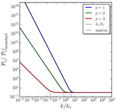
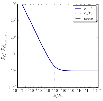
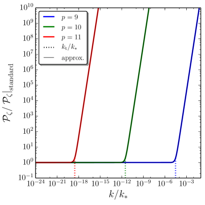
Figure 1: Numerical integration of the power spectrum in the case of a linear interaction with the environment, for different values of $p$ as indicated on the plots. The coloured lines represent the exact result while the black lines correspond to our analytical approximation (3.29)-(3.36) (because of the perfect overlap they are difficult to distinguish). The vertical dotted lines indicate the position of the transition scale $k_{\mathrm{t}}$ as given in Eqs. (3.38). The values chosen for the parameters are $\epsilon_{1*}=10^{-4}$, $\epsilon_{2*}=1-0.96-2\epsilon_{1*}$ (such that $n_{\scriptscriptstyle{\mathrm{S}}}\simeq 0.96$ in the standard branch), $H_{*}\ell_{\mathrm{E}}=10^{-3}$, $k_{\gamma}/k_{*}=10^{-3}$, and $\Delta N_{*}=50$.

In order to check the validity of the above calculations, we have numerically integrated the power spectrum for different values of $p$, and compared the result to our analytical approximations. The comparison is displayed in Fig. 1, where one can check that the analytical approximations (3.29)-(3.36) match very well the numerical result (because of the perfect overlap they can in fact not even be distinguished).

The structure of Eq. (3.14) implies that the power spectrum in the presence of decoherence is made of two branches, the standard, almost scale-invariant one, and a new branch which strongly deviates from scale invariance (except for the case $p\simeq 5$ discussed below). The scale $k_{\mathrm{t}}$ at which the transition between the two branches occurs is such that ${\cal A}_{i}(k_{\mathrm{t}})\sim 1$, and Eqs. (3.37), (3.32) and (3.35) give rise to

$$\frac{k_{\mathrm{t}}}{k_{*}}\biggl{|}_{1} \simeq\left(\frac{k_{\gamma}}{k_{*}}\right)^{-\frac{2}{3}}\exp\left\{-\frac{\Delta N_{*}}{3}\left[p-3-\frac{2(1+\nu)}{1+\epsilon_{1}}\right]\right\},$$ (3.38)

$$\frac{k_{\mathrm{t}}}{k_{*}}\biggl{|}_{2} \simeq\left(\frac{k_{\gamma}}{k_{*}}\right)^{-\frac{2}{p-5}},$$

$$\frac{k_{\mathrm{t}}}{k_{*}}\biggl{|}_{3} \simeq\left(\frac{k_{\gamma}}{k_{*}}\right)^{-\frac{2}{p-5}}\left(H_{*}\ell_{\mathrm{E}}\right)^{-\frac{p-4}{p-5}}\,,$$

where $\Delta N_{*}$ corresponds to $N-N_{*}$ evaluated at the end of inflation, i.e. $\Delta N_{*}=N_{\mathrm{end}}-N_{*}$.

More precisely, in the first case, i.e. when $p>8-3\epsilon_{1*}+\epsilon_{2*}$, Eq. (3.37) shows that the correction to the standard power spectrum scales as $k^{3}$ regardless of the value of $p$. This can be checked on the bottom-right panel of Fig. 1 where, for $p=9$, $10$ and $11$, the corrections grow for large values of $k$ (small scales) and have the same slope. Since we observe an almost scale-invariant power spectrum, the part $k>k_{\mathrm{t}}$ of the power spectrum has to be outside the observable window, $k_{\mathrm{t}}\gg k_{*}$. Together with Eq. (3.38), it gives rise to

$$\left.\frac{k_{\gamma}}{k_{*}}\right|_{1}\ll e^{-\frac{1}{2}\left(p-8+3\epsilon_{1*}-\epsilon_{2*}\right)\Delta N_{*}}\,.$$ (3.39)

Through Eq. (3.4), this directly constrains the interaction strength with the environment, to very small values.

The second case corresponds to $4-\epsilon_{1*}<p<8-3\epsilon_{1*}+\epsilon_{2*}$, and Eq. (3.32) implies that the correction scales as $k^{p-5}$, such that it modifies the power spectrum at $k>k_{\mathrm{t}}$ if $p>5$ and $k<k_{\mathrm{t}}$ if $p<5$ (the case $p=5$ is singular and is discussed separately below), with a $p$-dependent slope. This can be checked on the top-right and bottom-left panels of Fig. 1. For instance, for $p=4$ (top-right panel), ${\cal A}_{2}(k)\propto k^{-1}$ and, indeed, the correction grows on large scales. On the contrary, if we consider, say $p=6$ and $p=7$ (bottom-right panel), one has ${\cal A}_{2}(k)\propto k^{1}$ and ${\cal A}_{2}(k)\propto k^{2}$ respectively, and, indeed, the corrections now grow on small scales and with different slopes. In order for observed modes to lie outside the modified, non scale-invariant part of the power spectrum, one needs to have $k_{\mathrm{t}}\ll k_{*}$ for $p<5$ and $k_{\mathrm{t}}\gg k_{*}$ for $p>5$. In both cases, with Eq. (3.38) it leads to

$$\left.\frac{k_{\gamma}}{k_{*}}\right|_{2}\ll 1\,.$$ (3.40)

Finally, the third case is defined by $p<4-\epsilon_{1*}$. The scaling of ${\cal A}_{3}(k)$ is the same as for ${\cal A}_{2}(k)$ as can be checked on the top-left panel in Fig. 1. For instance, $p=2$ corresponds to ${\cal A}_{3}(k)\propto k^{-3}$ and $p=3$ to ${\cal A}_{2}(k)\propto k^{-2}$. Observational constraints on scale invariance impose $k_{\mathrm{t}}\ll k_{*}$, which, with Eq. (3.38), translates into

$$\left.\frac{k_{\gamma}}{k_{*}}\right|_{3}\ll\left(H_{*}\ell_{\mathrm{E}}\right)^{\frac{4-p}{2}}\,.$$ (3.41)

Notice that the constraint $k_{\mathrm{t}}\ll k_{*}$ (when $p<5$) is conceptually different from the constraint $k_{\mathrm{t}}\gg k_{*}$ (when $p>5$). Indeed, in the former case, one removes the corrections to the power spectrum outside our observational window, while in the later case, one pushes the corrections to scales that are smaller than the ones probed in the CMB but that could still be of astrophysical interest.

3.1.7 Case of a heavy scalar field as the environment

As can be seen in Fig. 1, of particular interest is the case $p=5$, see the pink line in the bottom-left panel, where the power spectrum is almost scale invariant even in the modified branch. A crucial remark is that the microphysical example studied in Appendix B, where the environment is made of the degrees of freedom contained in a heavy test scalar field, precisely gives $p\simeq 5$. More precisely, from Eq. (2.22), one has $p=5-6m\epsilon_{1*}$ in that case. Let us study the observational predictions of this model in more details. Combining the standard expression of the power spectrum, namely

$$\mathcal{P}_{\zeta}|_{\mathrm{standard}}=\frac{H_{*}^{2}}{8\pi^{2}\epsilon_{1}M_{\scriptscriptstyle{\mathrm{Pl}}}^{2}}\left[1-2(C+1)\epsilon_{1*}-C\epsilon_{2*}-(2\epsilon_{1*}+\epsilon_{2*})\ln\left(\frac{k}{k_{*}}\right)\right],$$ (3.42)

where $C=\gamma_{\mathrm{E}}+\ln 2-2\simeq-0.7296$ is a numerical constant, with Eqs. (3.14) and (3.26), one has

$$\mathcal{P}_{\zeta}= \frac{H_{*}^{2}\left(1+\frac{\pi}{6}\frac{k_{\gamma}^{2}}{k_{*}^{2}}\right)}{8\pi^{2}\epsilon_{1}M_{\scriptscriptstyle{\mathrm{Pl}}}^{2}}\left\{1-\frac{2\left(C+1\right)+\frac{\pi}{9}\frac{k_{\gamma}^{2}}{k_{*}^{2}}\left[2-3C+3\left(3C-1\right)m\right]}{1+\frac{\pi}{6}\frac{k_{\gamma}^{2}}{k_{*}^{2}}}\epsilon_{1*}\right.$$ (3.43)

$$\left.-\left[C+\frac{\frac{\pi}{6}\frac{k_{\gamma}^{2}}{k_{*}^{2}}}{3\left(1+\frac{\pi}{6}\frac{k_{\gamma}^{2}}{k_{*}^{2}}\right)}\right]\epsilon_{2*}-\left[2\epsilon_{1*}+\epsilon_{2*}+\frac{\frac{\pi}{6}\frac{k_{\gamma}^{2}}{k_{*}^{2}}\left(6m-2\right)}{1+\frac{\pi}{6}\frac{k_{\gamma}^{2}}{k_{*}^{2}}}\epsilon_{1*}\right]\ln\left(\frac{k}{k_{*}}\right)\right\}\,.$$

In this expression, recall that $k_{\gamma}/k_{*}$ is given by Eq. (3.5). This formula differs in two ways from the standard one (3.42). First, the amplitude is no longer a function of the inflationary energy scale $H_{*}$ and the first slow-roll parameter $\epsilon_{1*}$ only, but now also depends on the ratio $k_{\gamma}/k_{*}$. If one assumes that tensor perturbations are not affected by the presence of the environment and that their power spectrum is still given by the standard formula $\mathcal{P}_{h}\simeq 2H_{*}^{2}/(\pi^{2}M_{\scriptscriptstyle{\mathrm{Pl}}}^{2})$, the tensor-to-scalar ratio $r\equiv\mathcal{P}_{h}/\mathcal{P}_{\zeta}$, which is the standard case in given by $\left.r\right|_{\mathrm{standard}}=16\epsilon_{1*}$, now reads

$$r=\frac{\left.r\right|_{\mathrm{standard}}}{1+\frac{\pi}{6}\frac{k_{\gamma}^{2}}{k_{*}^{2}}}\,.$$ (3.44)

When $k_{\gamma}/k_{*}\ll 1$, one recovers the standard result, otherwise $r$ is reduced compared to the free theory. Second, the spectral index $n_{\scriptscriptstyle{\mathrm{S}}}\equiv 1+\mathrm{d}\ln\mathcal{P}_{\zeta}/\mathrm{d}\ln k$ is also modified, and instead of the standard formula $\left.n_{\scriptscriptstyle{\mathrm{S}}}\right|_{\mathrm{standard}}=1-2\epsilon_{1*}-\epsilon_{2*}$, we now have

$$n_{\scriptscriptstyle{\mathrm{S}}}=\left.n_{\scriptscriptstyle{\mathrm{S}}}\right|_{\mathrm{standard}}-\frac{\frac{\pi}{6}\frac{k_{\gamma}^{2}}{k_{*}^{2}}}{1+\frac{\pi}{6}\frac{k_{\gamma}^{2}}{k_{*}^{2}}}\left(6m-2\right)\epsilon_{1*}\,.$$ (3.45)

When $k_{\gamma}/k_{*}\ll 1$, one recovers the standard result $n_{\scriptscriptstyle{\mathrm{S}}}\simeq\left.n_{\scriptscriptstyle{\mathrm{S}}}\right|_{\mathrm{standard}}$ but if $k_{\gamma}/k_{*}\gg 1$, one obtains $n_{\scriptscriptstyle{\mathrm{S}}}\simeq\left.n_{\scriptscriptstyle{\mathrm{S}}}\right|_{\mathrm{standard}}-(6m-2)\epsilon_{1*}$. The shift in the spectral index $\Delta n_{\scriptscriptstyle{\mathrm{S}}}$ is negative (at least for $m>1/3$) and proportional to $\epsilon_{1*}$, so it is still compatible with quasi scale invariance but it may have consequences for particular models of inflation.

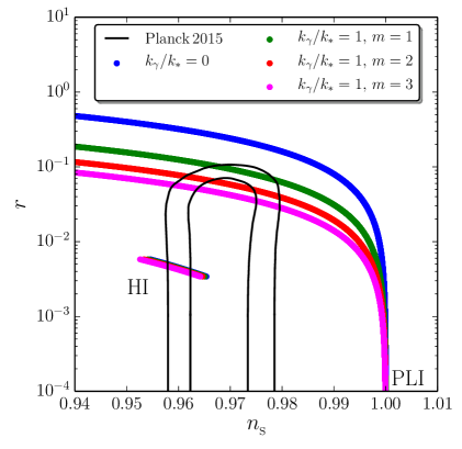
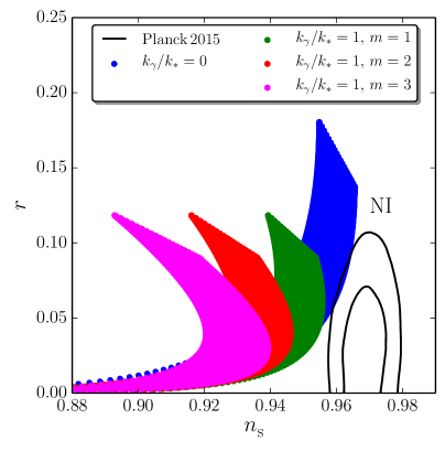
Figure 2: Spectral index $n_{\scriptscriptstyle{\mathrm{S}}}$ and tensor-to-scalar ratio $r$ for three single-field models of inflation, Higgs inflation (or the Starobinsky model) “HI” and power-law inflation “PLI” in the left panel, and natural inflation “NI” in the right panel. The black lines correspond to the one- and two-sigma contours obtained from the Planck 2015 $TT$ data combined with the high-$\ell$ $C_{\ell}^{TE}+C_{\ell}^{EE}$ likelihood and the low-$\ell$ temperature plus polarisation likelihood (PlanckTT,TE,EE+lowTEB in the notations of LABEL:Aghanim:2015xee) together with the BICEP2-Keck/Planck likelihood described in LABEL:Ade:2015tva. The blue disks correspond to the standard results in absence of decoherence, while the green, red and pink disks correspond to the modified power spectrum (3.43) with $k_{\gamma}/k_{*}=1$, for $m=1$, $2$ and $3$ respectively.

To illustrate this result, in Fig. 2 we have displayed the spectral index and the tensor-to-scalar ratio predicted by three single-field models of inflation: Higgs inflation [65] (or the Starobinsky model [7], HI) where the potential is given by $V(\phi)\propto[1-\exp(-\mathchoice{{\hbox{$\displaystyle\sqrt{2/3\,}$}\lower 0.4pt\hbox{\vrule height=7.5pt,depth=-6.00003pt}}}{{\hbox{$\textstyle\sqrt{2/3\,}$}\lower 0.4pt\hbox{\vrule height=7.5pt,depth=-6.00003pt}}}{{\hbox{$\scriptstyle\sqrt{2/3\,}$}\lower 0.4pt\hbox{\vrule height=5.25pt,depth=-4.20003pt}}}{{\hbox{$\scriptscriptstyle\sqrt{2/3\,}$}\lower 0.4pt\hbox{\vrule height=3.75pt,depth=-3.00002pt}}}\phi/M_{\scriptscriptstyle{\mathrm{Pl}}})]^{2}$, power-law inflation [66] (PLI) where $V(\phi)\propto\exp(-\alpha\phi/M_{\scriptscriptstyle{\mathrm{Pl}}})$, and natural inflation [67] (NI) where $V(\phi)\propto 1+\cos(\phi/f)$. The predictions are calculated with the ASPIC library [68, 69], where the free parameters appearing in the potential are varied together with the reheating temperature according to the priors of LABEL:Martin:2013nzq, and one assumes the averaged equation-of-state parameter during reheating to vanish. The black lines are the one- and two-sigma contours of the BICEP2-Keck/Planck 2015 likelihood [64, 14]. The blue disks correspond to the standard predictions (3.42), while the green, red and pink disks correspond to the modified predictions (3.43) $k_{\gamma}/k_{*}=1$, for $m=1$, $2$ and $3$ respectively. For the plateau model of Higgs inflation, because the predicted tensor-to-scalar ratio in the free theory is small, $\epsilon_{1*}$ is small and the shift in the spectral index is also small, such that the model still provides a good fit to the data in the presence of decoherence. For power-law inflation, in the absence of decoherence the model is strongly disfavoured, since it predicts a too large value for $n_{\scriptscriptstyle{\mathrm{S}}}$ when $r$ is sufficiently small. In the presence of decoherence however, the decrease in the value of both $n_{\scriptscriptstyle{\mathrm{S}}}$ and $r$ is such that the model becomes viable for some values of its free parameter $\alpha$. For natural inflation, the standard version of the model is disfavoured since it predicts a too small value for the spectral index. By further decreasing the spectral index, decoherence makes it worse and the model is even more disfavoured.

One concludes that for the interaction model proposed in Appendix B, the observational constraint on the interaction strength, here parametrised by $k_{\gamma}/k_{*}$, depends on the specific model of inflation. For models predicting the right value of the spectral index and very low values for the tensor-to-scalar ratio, such as Higgs inflation, decoherence does not change much the predictions and as a result there is no strong constraint on $k_{\gamma}/k_{*}$. For models predicting too large values for the spectral index, such as power-law inflation, the model becomes viable only in the presence of decoherence and observations place a lower bound on the interaction strength. On the contrary, for models predicting too small values for the spectral index, such as natural inflation, or models predicting values for the spectral index that are in agreement with the data and values for the tensor-to-scalar ratio that are not far from the current upper bound, decoherence can only make the model worse, and observations impose an upper bound on the interaction strength.

3.2 Quadratic interaction

Let us now consider the case where the system couples quadratically to the environment, $\hat{A}(\bm{x})=\hat{v}^{2}(\bm{x})$, i.e. $n=2$ in Eq. (2.14). Contrary to the case of linear interactions, because of mode coupling, the Lindblad equation (2.16) does not decouple into a set of independent Lindblad equations for each Fourier mode, and cannot be solved entirely. However, the power spectrum can still be calculated by making use of the technique presented in Sec. 3.1.4.

3.2.1 Two-point correlation functions

Let us start by deriving the equation of motion for the two-point correlation functions. Using the fact that the Fourier transform of a squared function is the convolution product of its Fourier transform, namely

$$\hat{v}^{2}(\eta,{\bm{x}})=\frac{1}{(2\pi)^{3}}\int_{\mathbb{R}^{3}}{\mathrm{d}}^{3}{\bm{k}}^{\prime}\,{\mathrm{d}}^{3}{\bm{p}}\,\hat{v}_{\bm{k}^{\prime}}\hat{v}_{\bm{p}-\bm{k}^{\prime}}\,\mathrm{e}^{i{\bm{p}}\cdot{\bm{x}}},$$ (3.46)

one obtains that Eq. (2.25) leads to

$$\frac{\mathrm{d}\left\langle\hat{\rho}_{v}\hat{O}\right\rangle}{\mathrm{d}\eta}= -i\left\langle\left[\hat{O},\hat{H}_{v}\right]\right\rangle+\left\langle\frac{\partial\hat{O}}{\partial\eta}\hat{\rho}_{v}\right\rangle$$ (3.47)

$$-\frac{\gamma}{2(2\pi)^{3/2}}\int_{\mathbb{R}^{3}}\mathrm{d}^{3}\bm{k}\,\mathrm{d}^{3}{\bm{k}}^{\prime}\,\mathrm{d}^{3}{\bm{q}}\,\tilde{C}_{R}(\bm{k})\left\langle\left[\left[\hat{O},\hat{v}_{{\bm{k}}^{\prime}}\hat{v}_{{\bm{k}}-{\bm{k}}^{\prime}}\right],\hat{v}_{{\bm{q}}}\hat{v}_{-{\bm{k}}-{\bm{q}}}\right]\hat{\rho}_{v}\right\rangle\,.$$

As explained in Sec. 3.1.4, one can derive the equations of motion for one-point correlators and, as before, find that, in agreement with Ehrenfest theorem, the standard equations are unmodified, see Eqs. (3.16). For two-point correlators, as in Sec. 3.1.4, only the equation for $\langle\hat{p}_{{\bm{k}}_{1}}\hat{p}_{{\bm{k}}_{2}}\rangle$ is changed and one finds

$$\frac{\mathrm{d}}{\mathrm{d}\eta}\left\langle\hat{v}_{{\bm{k}}_{1}}\hat{v}_{{\bm{k}}_{2}}\right\rangle =\left\langle\hat{v}_{{\bm{k}}_{1}}\hat{p}_{{\bm{k}}_{2}}+\hat{p}_{{\bm{k}}_{1}}\hat{v}_{{\bm{k}}_{2}}\right\rangle,$$ (3.48)

$$\frac{\mathrm{d}}{\mathrm{d}\eta}\left\langle\hat{v}_{{\bm{k}}_{1}}\hat{p}_{{\bm{k}}_{2}}\right\rangle =\left\langle\hat{p}_{{\bm{k}}_{1}}\hat{p}_{{\bm{k}}_{2}}\right\rangle-\omega^{2}(k_{2})\left\langle\hat{v}_{{\bm{k}}_{1}}\hat{v}_{{\bm{k}}_{2}}\right\rangle,$$

$$\frac{\mathrm{d}}{\mathrm{d}\eta}\left\langle\hat{p}_{{\bm{k}}_{1}}\hat{v}_{{\bm{k}}_{2}}\right\rangle =\left\langle\hat{p}_{{\bm{k}}_{1}}\hat{p}_{{\bm{k}}_{2}}\right\rangle-\omega^{2}(k_{1})\left\langle\hat{v}_{{\bm{k}}_{1}}\hat{v}_{{\bm{k}}_{2}}\right\rangle,$$

$$\frac{\mathrm{d}}{\mathrm{d}\eta}\left\langle\hat{p}_{{\bm{k}}_{1}}\hat{p}_{{\bm{k}}_{2}}\right\rangle =-\omega^{2}(k_{2})\left\langle\hat{p}_{{\bm{k}}_{1}}\hat{v}_{{\bm{k}}_{2}}\right\rangle-\omega^{2}(k_{1})\left\langle\hat{v}_{{\bm{k}}_{1}}\hat{p}_{{\bm{k}}_{2}}\right\rangle$$

$$+\frac{4\gamma}{(2\pi)^{3/2}}\int\mathrm{d}^{3}{\bm{k}}\,\tilde{C}_{R}(\bm{k})\left\langle\hat{v}_{{\bm{k}}+{\bm{k}}_{1}}\hat{v}_{-{\bm{k}}+{\bm{k}}_{2}}\right\rangle.$$

An important remark is that the term involving $\gamma$ is not explicitly proportional to $\delta({\bm{k}}_{1}+{\bm{k}}_{2})$ as was the case for linear interactions, where the presence of the Dirac function guaranteed that the Lindblad term preserved statistical homogeneity. One may therefore be concerned that the above system generates violations to statistical homogeneity. However, if the system is solved through a perturbative expansion in $\gamma$, during the first iteration the Lindblad term contains the correlator $\langle\hat{v}_{{\bm{k}}+{\bm{k}}_{1}}\hat{v}_{-{\bm{k}}+{\bm{k}}_{2}}\rangle$ evaluated in the free theory, which is proportional to $\delta(\bm{k}_{1}+\bm{k}_{2})$. This guarantees that the solution that is obtained at the first iteration is statistically homogeneous. Since it sources the equation at the second iteration, the solution is again statistically homogeneous, so on and so forth. The result is therefore statistically homogeneous, and Eq. (3.48) admits a solution of the form given by Eq. (3.18). If $\tilde{C}_{R}$ is also isotropic, $\tilde{C}_{R}(\bm{k})=\tilde{C}_{R}(k)$, the system for isotropic solutions then reduces to

$$\frac{\mathrm{d}P_{vv}(k)}{\mathrm{d}\eta} =P_{vp}(k)+P_{pv}(k),$$ (3.50)

$$\frac{\mathrm{d}P_{vp}(k)}{\mathrm{d}\eta} =\frac{\mathrm{d}P_{pv}(k)}{\mathrm{d}\eta}=P_{pp}(k)-w^{2}(k)P_{vv}(k),$$

$$\frac{\mathrm{d}P_{pp}(k)}{\mathrm{d}\eta} =-\omega^{2}(k)\left[P_{pv}(k)+P_{vp}(k)\right]+\frac{4\gamma}{(2\pi)^{3/2}}\int_{\mathbb{R}^{3}}\mathrm{d}^{3}{\bm{k}}^{\prime}\,\tilde{C}_{R}\left(k^{\prime}\right)P_{vv}\left(\left|\bm{k}^{\prime}+\bm{k}\right|\right).$$

As was done in the linear interaction case, one can combine the above equations in order to get a third order equation for $P_{vv}$ only,

$$P_{vv}^{\prime\prime\prime}+4\omega^{2}P_{vv}^{\prime}+4\omega^{\prime}\omega P_{vv}-\frac{8\gamma}{(2\pi)^{3/2}}\int_{\mathbb{R}^{3}}\mathrm{d}^{3}{\bm{k}}^{\prime}\,\tilde{C}_{R}\left({k}^{\prime}\right)P_{vv}\left(\left|\bm{k}^{\prime}+\bm{k}\right|\right)=0\,.$$ (3.51)

Compared with the corresponding equation (3.21) for linear interactions, where the power spectrum is sourced by the Fourier transform of the environment correlation function, in the present case it is sourced by the convolution product of the Fourier transform of the environment correlation function with the power spectrum itself. This makes clear that, as announced, quadratic interactions yield mode coupling, since the power spectrum at a given mode is sourced by its value at all other modes.

As was mentioned for the linear case, our technique can still be employed if $\hat{A}$ involves $\hat{p}$. In the quadratic case discussed here, this either implies $\hat{A}=\hat{p}^{2}$ or $\hat{A}=\hat{v}\hat{p}$. In that situtation, $P_{vv}$ obeys the same equation as Eq. (3.51), with a different source function that we do not give here since its concrete form is not especially illuminating but that can be readily obtained.

3.2.2 Solving the equation for the power spectrum

The third-order differential equation for the power spectrum $P_{vv}$, Eq. (3.51), is of the form

$$P_{vv}^{\prime\prime\prime}+4\omega^{2}P_{vv}^{\prime}+4\omega\omega^{\prime}P_{vv}=S_{2}\,,$$ (3.52)

where the source $S_{2}$ is a function of time that involves the power spectrum $P_{vv}$ itself evaluated at all scales, namely

$$S_{2}\left(\bm{k},\eta\right)=\frac{8\gamma}{(2\pi)^{3/2}}\int_{\mathbb{R}^{3}}\mathrm{d}^{3}{\bm{k}}^{\prime}\,\tilde{C}_{R}\left({k}^{\prime}\right)P_{vv}\left(\left|\bm{k}^{\prime}+\bm{k}\right|\right)\,.$$ (3.53)

This is therefore an integro-differential equation, that couples all modes together, and that is very difficult to solve in full generality. However, at leading order in $\gamma$, one can use the free theory to calculate $S_{2}$, which becomes a fixed function of time. Then, Eq. (3.52) is turned into an ordinary differential equation that can be solved as we now explain. If one wants to go to higher orders in $\gamma$, one can repeat the procedure and embed it in a recursive expansion in $\gamma$, but that would be inconsistent with the standard derivation of the Lindblad equation, see Appendix A, which is valid at linear order in $\gamma$ only.

Inspired by the fact that Eq. (3.9) provides a solution to Eq. (3.21), let us introduce the function ${\cal S}_{\bm{k}}$ defined by

$$\mathcal{S}_{\bm{k}}\left(\eta\right)=-\frac{2}{\left(v^{*}_{\bm{k}}v_{\bm{k}}^{\prime}-v^{\prime*}_{\bm{k}}v_{\bm{k}}\right)^{2}}\int_{\eta_{0}}^{\eta}S_{2}\left(\eta^{\prime}\right)\mathrm{Im}^{2}\left[v_{\bm{k}}\left(\eta^{\prime}\right)v^{*}_{\bm{k}}\left(\eta\right)\right]\mathrm{d}\eta^{\prime}\,,$$ (3.54)

where $v_{\bm{k}}(\eta)$ is a mode function, that is to say a solution of the Mukhanov-Sasaki equation $v^{\prime\prime}_{\bm{k}}+\omega^{2}v_{\bm{k}}=0$. Since the Wronskian of $v_{\bm{k}}$ is conserved through the Mukhanov-Sasaki equation, the factor in front the integral in Eq. (3.54) is a constant. Using similar techniques as the ones used below Eq. (3.21), it is straightforward to check that $\mathcal{S}_{\bm{k}}$ is a particular solution of the equation of motion (3.52) for $P_{vv}$.

In fact, one can show that this particular solution is independent of the mode function $v_{\bm{k}}(\eta)$ one has chosen. Indeed, $\mathcal{S}_{\bm{k}}(\eta)$ is the solution of Eq. (3.52) that, as can be shown from Eq. (3.54), satisfies $\mathcal{S}_{\bm{k}}(\eta_{0})=\mathcal{S}^{\prime}_{\bm{k}}(\eta_{0})=\mathcal{S}^{\prime\prime}_{\bm{k}}(\eta_{0})=0$. It is therefore unique. In practice, to evaluate it, one can use the Bunch-Davies normalised mode function, for which $v_{\bm{k}}^{*}v_{\bm{k}}-v_{\bm{k}}^{\prime*}v_{\bm{k}}=i$, but the result is independent of that choice, and $\mathcal{S}_{\bm{k}}(\eta)$ therefore carries a single integration constant, namely $\eta_{0}$. The full solution can be obtained by adding the solution of the homogeneous equation (i.e. without the source term) $P_{vv}^{\prime\prime\prime}+4\omega^{2}P_{vv}^{\prime}+4\omega\omega^{\prime}P_{vv}=0$. As already mentioned for the linear case, one can check that $v_{\bm{k}}(\eta)v^{*}_{\bm{k}}(\eta)$ satisfies this equation if $v_{\bm{k}}$ is a solution [not necessarily the same as the one used to write down Eq. (3.54)] of the mode equation. The complete solution can then be expressed as

$$P_{vv}\left(k\right)=|v_{\bm{k}}|^{2}+\mathcal{S}_{\bm{k}}.$$ (3.55)

If one sets the mode function appearing in the first term of the right-hand side of Eq. (3.55) to the Bunch-Davies normalised one, $P_{vv}$ matches the Bunch-Davies result in the infinite past if $\eta_{0}=-\infty$, and this leads to

$$P_{vv}=v_{\bm{k}}\left(\eta\right)v^{*}_{\bm{k}}\left(\eta\right)+2\int_{-\infty}^{\eta}S_{2}\left(\eta^{\prime}\right)\mathrm{Im}^{2}\left[v_{\bm{k}}\left(\eta^{\prime}\right)v^{*}_{\bm{k}}\left(\eta\right)\right]\mathrm{d}\eta^{\prime}\,.$$ (3.56)

In this expression, let us stress that $v_{\bm{k}}$ is now Bunch-Davies normalised. Notice that since this does not rely on the concrete form of $S_{2}$, Eq. (3.56) is a solution of Eq. (3.52) for any source function. In particular, if the source term is given by $S_{1}$, see Eq. (3.22), then Eq. (3.54) for $\mathcal{S}_{\bm{k}}$ reduces to Eq. (3.9) that defines ${\cal J}_{\bm{k}}$, and Eq. (3.55) matches Eq. (3.13).

3.2.3 Calculation of the source term

The next step is to calculate the source term, that is to say the convolution product between the power spectrum in the free theory and the Fourier transform of the environment correlator. This is done in details in Appendix D.1 and here, we simply quote the result. By performing the angular integration, one can first show that

$$\int_{\mathbb{R}^{3}}\mathrm{d}^{3}{\bm{k}}^{\prime}\,\tilde{C}_{R}\left(k^{\prime}\right)P_{vv}\left(\left|\bm{k}^{\prime}+\bm{k}\right|\right) =\frac{\pi}{k}\int_{0}^{\infty}\mathrm{d}p\,p\,P_{vv}(p)\int_{\left(k-p\right)^{2}}^{\left(k+p\right)^{2}}\mathrm{d}z\,\tilde{C}_{R}\left(\mathchoice{{\hbox{$\displaystyle\sqrt{z\,}$}\lower 0.4pt\hbox{\vrule height=4.30554pt,depth=-3.44446pt}}}{{\hbox{$\textstyle\sqrt{z\,}$}\lower 0.4pt\hbox{\vrule height=4.30554pt,depth=-3.44446pt}}}{{\hbox{$\scriptstyle\sqrt{z\,}$}\lower 0.4pt\hbox{\vrule height=3.01389pt,depth=-2.41113pt}}}{{\hbox{$\scriptscriptstyle\sqrt{z\,}$}\lower 0.4pt\hbox{\vrule height=2.15277pt,depth=-1.72223pt}}}\right)\,,$$ (3.57)

see Eq. (D.3). The integral over $p$ contains a UV part ($p>aH$, sub-Hubble scales) and an IR part ($p<aH$, super-Hubble scales).

The UV part is finite and subdominant at late time. In any case, as usually done, it is regularised away by adiabatic subtraction [72, 73], which amounts to setting the upper bound of the integral over $p$ in Eq. (3.57) to the comoving Hubble scale $-1/\eta$.

The IR part is divergent, and can be regularised by imposing an IR cutoff, that corresponds to the comoving Hubble scale at the onset of inflation and that we call $-1/\eta_{\mathrm{IR}}$. In the integral over $z$, $\tilde{C}_{R}$ is such that it vanishes when its argument is larger than the comoving correlation wavenumber of the environment, $a/\ell_{\mathrm{E}}$, and goes to a constant value in the opposite limit. Since the integral over $p$ is now restricted to super-Hubble modes, $p<aH$, and given that we assumed $\ell_{\mathrm{E}}\ll H^{-1}$ when deriving the Lindblad equation (at least if $\ell_{\mathrm{E}}\sim t_{\mathrm{c}}$, see Appendix A), one has $p\ll a/\ell_{\mathrm{E}}$. Two cases can then be distinguished. If $k\ll a/\ell_{\mathrm{E}}$, both $|k-p|$ and $k+p$ are much smaller than $a/\ell_{\mathrm{E}}$, and $\tilde{C}_{R}(\mathchoice{{\hbox{$\displaystyle\sqrt{z\,}$}\lower 0.4pt\hbox{\vrule height=4.30554pt,depth=-3.44446pt}}}{{\hbox{$\textstyle\sqrt{z\,}$}\lower 0.4pt\hbox{\vrule height=4.30554pt,depth=-3.44446pt}}}{{\hbox{$\scriptstyle\sqrt{z\,}$}\lower 0.4pt\hbox{\vrule height=3.01389pt,depth=-2.41113pt}}}{{\hbox{$\scriptscriptstyle\sqrt{z\,}$}\lower 0.4pt\hbox{\vrule height=2.15277pt,depth=-1.72223pt}}})$ is constant over its integration range. If $k\gg a/\ell_{\mathrm{E}}$, both $|k-p|$ and $k+p$ are much larger than $a/\ell_{\mathrm{E}}$, and $\tilde{C}_{R}(\mathchoice{{\hbox{$\displaystyle\sqrt{z\,}$}\lower 0.4pt\hbox{\vrule height=4.30554pt,depth=-3.44446pt}}}{{\hbox{$\textstyle\sqrt{z\,}$}\lower 0.4pt\hbox{\vrule height=4.30554pt,depth=-3.44446pt}}}{{\hbox{$\scriptstyle\sqrt{z\,}$}\lower 0.4pt\hbox{\vrule height=3.01389pt,depth=-2.41113pt}}}{{\hbox{$\scriptscriptstyle\sqrt{z\,}$}\lower 0.4pt\hbox{\vrule height=2.15277pt,depth=-1.72223pt}}})$ vanishes over its full integration range. This means that in Eq. (3.57), one can simply replace $\tilde{C}_{R}(\mathchoice{{\hbox{$\displaystyle\sqrt{z\,}$}\lower 0.4pt\hbox{\vrule height=4.30554pt,depth=-3.44446pt}}}{{\hbox{$\textstyle\sqrt{z\,}$}\lower 0.4pt\hbox{\vrule height=4.30554pt,depth=-3.44446pt}}}{{\hbox{$\scriptstyle\sqrt{z\,}$}\lower 0.4pt\hbox{\vrule height=3.01389pt,depth=-2.41113pt}}}{{\hbox{$\scriptscriptstyle\sqrt{z\,}$}\lower 0.4pt\hbox{\vrule height=2.15277pt,depth=-1.72223pt}}})$ by $\tilde{C}_{R}(k)$, and one obtains

$$\int_{\mathbb{R}^{3}}\mathrm{d}^{3}{\bm{k}}^{\prime}\,\tilde{C}_{R}\left(k^{\prime}\right)P_{vv}\left(\left|\bm{k}^{\prime}+\bm{k}\right|\right) \simeq 4\pi\tilde{C}_{R}\left(k\right)\int_{-1/\eta_{\mathrm{IR}}}^{-1/\eta}\mathrm{d}pp^{2}P_{vv}\left(p\right)\,.$$ (3.58)

In Appendix D.1, it is shown how this formula arises as a leading order expansion in $H\ell_{\mathrm{E}}$ starting from the ansatz (2.19), here we simply gave a heuristic argument. Finally, on super-Hubble scales and neglecting slow-roll corrections, the power spectrum in the free theory is given by $P_{vv}(p)=(2p)^{-1}(-p\eta)^{-2}$. Plugging this formula into Eq. (3.58), one is led to

$$\int\mathrm{d}^{3}{\bm{k}}^{\prime}\,\tilde{C}_{R}\left(k^{\prime}\right)P_{vv}\left(\left|\bm{k}^{\prime}+\bm{k}\right|\right) \simeq\frac{2\pi}{\eta^{2}}\tilde{C}_{R}\left(k\right)\ln\left(\frac{\eta_{\mathrm{IR}}}{\eta}\right)\,.$$ (3.59)

Notice that this expression was obtained neglecting all slow-roll corrections. Indeed, since the integral of the power spectrum over all modes appears in the source function, a slow-roll expansion around the pivot scale $k_{*}$ cannot be used consistently to describe the entire set of modes, and one would have to specify the details of the inflationary potential over the entire inflating domain [74] in order to calculate the source term beyond the de-Sitter limit. For this reason, we will ignore all following slow-roll corrections since their inclusion would be inconsistent. A more refined calculation would have to be carried out on a model-by-model basis. From Eqs. (3.51) and (3.59), the source function is then given by

$$S_{2}\left(\eta\right)=\frac{8\gamma}{\mathchoice{{\hbox{$\displaystyle\sqrt{2\pi\,}$}\lower 0.4pt\hbox{\vrule height=6.44444pt,depth=-5.15558pt}}}{{\hbox{$\textstyle\sqrt{2\pi\,}$}\lower 0.4pt\hbox{\vrule height=6.44444pt,depth=-5.15558pt}}}{{\hbox{$\scriptstyle\sqrt{2\pi\,}$}\lower 0.4pt\hbox{\vrule height=4.51111pt,depth=-3.6089pt}}}{{\hbox{$\scriptscriptstyle\sqrt{2\pi\,}$}\lower 0.4pt\hbox{\vrule height=3.22221pt,depth=-2.57779pt}}}\eta^{2}}\tilde{C}_{R}\left(k\right)\ln\left(\frac{\eta_{\mathrm{IR}}}{\eta}\right)\,.$$ (3.60)

3.2.4 Power spectrum and observational constraints

The final step consists in inserting this source with Eq. (2.27) into Eq. (3.56), which is done in Appendix D.2 and results in Eqs. (D.17)-(D.18). As for the linear case, the integrals can be performed in terms of generalised hypergeometric functions, see Eqs. (D.19) and (D.23). One can then simplify the expression of the power spectrum when evaluated on super-Hubble scales and using the fact that the environment has a correlation length much smaller than the Hubble radius, see Eq. (D.27). The modified power spectrum can still be defined by Eq. (3.14), where the equivalent of Eq. (3.15) for the quadratic interaction reads $\Delta{\cal P}_{\bm{k}}\equiv{\cal S}_{\bm{k}}/|v_{\bm{k}}|^{2}$. One finds that three regimes have to be distinguished. The first regime corresponds to when $p>6$, and gives

$$\left.\Delta{\cal P}_{\bm{k}}\right|_{1} \simeq\frac{8\sigma_{\gamma}}{27\pi}\left(\frac{k}{k_{*}}\right)^{3}e^{(p-6)\left(N-N_{*}\right)}\Biggl{[}\frac{1}{p^{2}}-\frac{2}{(p-3)^{2}}+\frac{1}{(p-6)^{2}}+\frac{18\left(N-N_{\mathrm{IR}}\right)}{p(p-3)(p-6)}\Biggr{]}.$$ (3.61)

The second case is when $2<p<6$, for which one has

$$\left.\Delta{\cal P}_{\bm{k}}\right|_{2}\simeq \frac{2^{p-1}(p-4)}{3p\Gamma(p-1)\sin(\pi p/2)}\sigma_{\gamma}\left(\frac{k}{k_{*}}\right)^{p-3}\biggl{[}N_{*}-N_{\mathrm{IR}}+\frac{1}{p-4}-\frac{2(p-1)}{p(p-2)}$$ (3.62)

$$-\frac{\pi}{2}\cot\left(\frac{\pi p}{2}\right)+\ln 2-\psi(p-2)+\ln\left(\frac{k}{k_{*}}\right)\biggr{]}.$$

Finally, the third regime is when $p<2$. In that case, the modification to the power spectrum reads

$$\left.\Delta{\cal P}_{\bm{k}}\right|_{3}\simeq \frac{4}{3}\frac{\left(H_{*}\ell_{\mathrm{E}}\right)^{p-2}}{\pi(2-p)}\sigma_{\gamma}\left(\frac{k}{k_{*}}\right)^{p-3}\biggl{[}\frac{1}{2-p}+N_{*}-N_{\mathrm{IR}}+\ln\left(H_{*}\ell_{\mathrm{E}}\right)+\ln\left(\frac{k}{k_{*}}\right)\biggr{]}.$$ (3.63)

In these expressions, $N-N_{\mathrm{IR}}\equiv\ln(\eta_{\mathrm{IR}}/\eta)$ denotes the number of $e$-folds elapsed since the onset of inflation, and we have introduced the dimensionless coefficient

$$\sigma_{\gamma}\equiv\bar{C}_{R}\frac{\ell_{\mathrm{E}}^{3}}{a_{*}^{3}}\gamma_{*}$$ (3.64)

that characterises the strength of the interaction with the environment. One notices that the cases $p=2$ and $p=6$ are singular and must be treated separately, giving rise to

$$\left.\Delta{\cal P}_{\bm{k}}\right|_{p=2}\simeq \frac{\sigma_{\gamma}}{18\pi}\left(\frac{k}{k_{*}}\right)^{-1}\Bigg{\{}12-\pi^{2}+12C\left(2+C\right)-12\ln^{2}\left(H_{*}\ell_{\mathrm{E}}\right)$$ (3.65)

$$+24\left[C+1-\ln\left(H_{*}\ell_{\mathrm{E}}\right)\right]\left[N_{*}-N_{\mathrm{IR}}+\ln\left(\frac{k}{k_{*}}\right)\right]\Bigg{\}}\,,$$

$$\left.\Delta{\cal P}_{\bm{k}}\right|_{p=6}\simeq \frac{\sigma_{\gamma}}{162\pi}\left(\frac{k}{k_{*}}\right)^{3}\Bigg{\{}2\pi^{2}-21-12C\left(1+2C\right)-12\left(3+4C\right)\left(N-N_{\mathrm{IR}}\right)$$

$$+12\left(1+4C\right)\left(N-N_{*}\right)+24\left(N-N_{*}\right)\left[2\left(N-N_{\mathrm{IR}}\right)-\left(N-N_{*}\right)\right]$$

$$-12\ln\left(\frac{k}{k_{*}}\right)\left[1+4\left(C+N_{*}-N_{\mathrm{IR}}\right)+2\ln\left(\frac{k}{k_{*}}\right)\right]\Bigg{\}}\,.$$

These analytical formulas are superimposed with a numerical integration of the power spectrum in Fig. 3, where one can check that the agreement is excellent (because of the perfect overlap, they are even hard to distinguish).

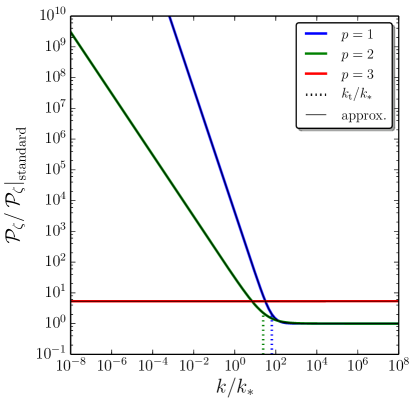
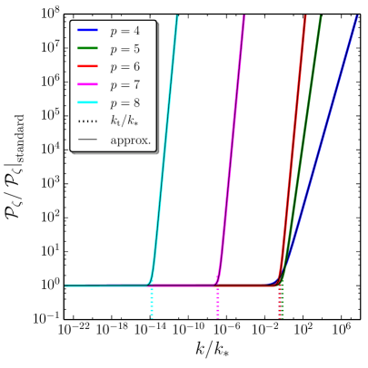
Figure 3: Power spectrum at the end of inflation, numerically integrated in the case of a quadratic interaction with the environment, for different values of $p$ as indicated on the plots. The coloured lines represent the exact result while the black lines correspond to our analytical approximations (3.61)-(3.65) (because of the perfect overlap they are difficult to distinguish). The vertical dotted lines indicate the position of the transition scale $k_{\mathrm{t}}$ defined by $\Delta\mathcal{P}_{\bm{k}_{\mathrm{t}}}=1$. The values chosen for the parameters are $H_{*}\ell_{\mathrm{E}}=10^{-3}$, $\sigma_{\gamma}=10^{-3}$, $\Delta N_{*}=50$, and $N_{{}_{\mathrm{T}}}=N_{\mathrm{end}}-N_{\mathrm{IR}}=10^{4}$.

As for the linear case, the power spectrum is made of two branches, one which matches the standard formula, and one where scale invariance is strongly broken (with the exception of the case $p=3$ that is discussed below separately). The transition between these two branches occurs at the scale $k_{\mathrm{t}}$ such that $\Delta\mathcal{P}_{\bm{k}_{\mathrm{t}}}=1$, and expressions similar to Eq. (3.38) can be derived from Eqs. (3.61)-(3.65) (we do not write them down here for display convenience but they are straightforward). A case-by-case analysis reveals several other similarities with the linear interaction results.

In the first case indeed, i.e. for large values of $p$, the power spectrum is not frozen on large scales and continues to increase, leading to a very large enhancement of the correction to the standard power spectrum at late time. The modified branch of the power spectrum scales as $k^{3}$, similarly to what was seen in Eq. (3.37). The requirement that observed modes are scale invariant, $k_{\mathrm{t}}\gg k_{*}$, leads to the constraint

$$\left.\sigma_{\gamma}\right|_{1}\ll\frac{e^{\left(6-p\right)\Delta N_{*}}}{N_{{}_{\mathrm{T}}}}\,,$$ (3.66)

where $N_{{}_{\mathrm{T}}}$ corresponds to $N-N_{\mathrm{IR}}$ evaluated at the end of inflation, i.e. $N_{{}_{\mathrm{T}}}=N_{\mathrm{end}}-N_{\mathrm{IR}}$ and stands for the total duration of inflation. Let us notice that the $1/N_{{}_{\mathrm{T}}}$ term originates from the last term in Eq. (3.61), which dominates when $N_{{}_{\mathrm{T}}}$ is very large.

In the second case, i.e. for intermediate values of $p$, the power spectrum is frozen on large scales and independent of the shape and correlation length of the environment correlator. This is again similar to the linear case. The power spectrum is modified on small scales, $k>k_{\mathrm{t}}$, if $p>3$, and on large scales, $k<k_{\mathrm{t}}$, if $p<3$. The requirement that the modified, non-scale invariant branch of the power spectrum is unobserved leads to

$$\left.\sigma_{\gamma}\right|_{2}\ll\frac{1}{N_{{}_{\mathrm{T}}}-\Delta N_{*}}\,.$$ (3.67)

The exception evading this constraint is the case $p=3$, where the power spectrum is almost scale invariant even in the modified branch. Strikingly, $p\simeq 3$ again corresponds to the scaling expected in the model proposed in Appendix B, where the environment is made of a heavy test scalar field. In this case, $\sigma_{\gamma}$ is related to the microphysical parameters of the model according to

$$\sigma_{\gamma}=128\left(\frac{37}{504\pi^{2}}\right)^{m}\frac{\left\{\left(2m-1\right)!!-\sigma\left(m\right)\left[\left(m-1\right)!!\right]^{2}\right\}^{3}}{\left[m^{2}\left(2m-3\right)!!\right]^{2}}\lambda^{2}\left(\frac{\mu}{M}\right)^{4-2m}\left(\frac{H_{*}}{M}\right)^{6m}\,,$$ (3.68)

where we have combined Eqs. (2.21), (2.22) and (3.64). Similarly to what was done in Sec. 3.1.7, constraints on $\gamma$ could be placed from the current observational bounds on $n_{\scriptscriptstyle{\mathrm{S}}}$ and $r$ within specific models of inflation, but this would require to include slow-roll corrections to the calculation of the source term, as explained above.

In the third case finally, i.e. for small values of $p$, the power spectrum freezes on large scales. The amplitude of the correction depends explicitly on the environment correlation length $\ell_{\mathrm{E}}$, and it scales with the wavenumber in the same manner as for intermediate values of $p$. This is again similar to the linear case. The power spectrum is modified on large scales $k<k_{\mathrm{t}}$, and requiring that the non scale-invariant part is unobserved leads to the constraint

$$\left.\sigma_{\gamma}\right|_{3}\ll\frac{\left(H\ell_{\mathrm{E}}\right)^{2-p}}{N_{{}_{\mathrm{T}}}-\Delta N_{*}+\ln\left(H_{*}\ell_{\mathrm{E}}\right)}\,.$$ (3.69)

4 Decoherence

In this section, we show how the addition of a non-unitary term in the evolution equation (2.16) of the density matrix of the system, that models the interaction with environmental degrees of freedoms, leads to the dynamical suppression of its off-diagonal elements in the basis of the eigenstates of the interaction operator (here the Mukhanov-Sasaki variable $\hat{v}$). Since this decoherence mechanism is thought to play a role in the quantum-to-classical transition of primordial cosmological perturbations, as explained in Sec. 1, we calculate the required strength of interaction that leads to decoherence at the end of inflation. We then compare this lower bound with the upper bound derived in the previous section from the requirement that quasi scale invariance is preserved. We thus identify the models for which successful decoherence occurs without spoiling standard observational predictions.

4.1 Linear interaction

In the case of linear interactions with the environment, in Sec. 3.1.2 (see also Appendix C) we have shown how Eq. (2.16) can be solved exactly and the density matrix was given in Eq. (LABEL:eq:finalrhomaintext). Since it is written in the basis of the eigenstates of $\hat{v}_{\bm{k}}$, through which the system couples to the environment, the suppression of its off-diagonal elements directly allows us to study decoherence.

4.1.1 Decoherence criterion

Let us consider an off-diagonal element of the density matrix $\hat{\rho}_{\bm{k}}^{s}$, away from the diagonal by a distance $\Delta v_{\bm{k}}$, that we write $\langle v_{{\bm{k}}}^{s}+\Delta v_{{\bm{k}}}/2|\hat{\rho}_{\bm{k}}^{s}|v_{{\bm{k}}}^{s}-\Delta v_{{\bm{k}}}/2\rangle$. From Eq. (LABEL:eq:finalrhomaintext), its amplitude can be expressed as

$$\left|\left\langle v_{{\bm{k}}}^{s}+\frac{\Delta v_{{\bm{k}}}}{2}\right|\hat{\rho}_{\bm{k}}^{s}\left|v_{{\bm{k}}}^{s}-\frac{\Delta v_{{\bm{k}}}}{2}\right\rangle\right|=\left|\left\langle v_{{\bm{k}}}^{s}\right|\hat{\rho}_{\bm{k}}^{s}\left|v_{{\bm{k}}}^{s}\right\rangle\right|\exp\left[-\frac{\delta_{\bm{k}}+\frac{1}{4}}{2}\frac{\Delta v_{{\bm{k}}}^{2}}{P_{vv}(k)}\right]\,,$$ (4.1)

where Eq. (3.13) has been used for the power spectrum $P_{vv}(k)$, and where we have introduced the parameter

$$\delta_{\bm{k}}(\eta) \equiv\mathcal{I}_{\bm{k}}\mathcal{J}_{\bm{k}}-\mathcal{K}_{\bm{k}}^{2}+\left|v_{\bm{k}}^{\prime}\right|^{2}\mathcal{J}_{\bm{k}}+\left|v_{\bm{k}}\right|^{2}\mathcal{I}_{\bm{k}}-{\left|v_{\bm{k}}\right|^{2}}^{\prime}\mathcal{K}_{\bm{k}}\,.$$ (4.2)

In Eq. (4.1), the factor $1/4$ has been separated out from the definition of $\delta_{\bm{k}}$ since it is present even in the absence of interactions with the environment (contrary to $\delta_{\bm{k}}$), such that $\delta_{\bm{k}}$ characterises the additional decrease of the off-diagonal elements produced by the environment. Successful decoherence is characterised by the condition $\delta_{\bm{k}}\gg 1$, which can be justified by either of the three following reasons.

First, the typical distance between two realisations $v_{\bm{k}}^{s,(1)}$ and $v_{\bm{k}}^{s,(2)}$ of the Mukhanov-Sasaki variable $v_{\bm{k}}$ is by definition given by the square root of its expected second moment, $\textstyle\sqrt{P_{vv}(k)\,}$ . If one replaces $\Delta v_{\bm{k}}$ by $\textstyle\sqrt{P_{vv}(k)\,}$  in Eq. (4.1), one can see that a large suppression of the off-diagonal element corresponds to a large value of $\delta_{\bm{k}}$.

Second, $\delta_{\bm{k}}$ appears in Eq. (4.1) added to $1/4$, which corresponds to the standard decrease of the off-diagonal term in the absence of an environment. It seems therefore natural to compare the environment-induced suppression of the off-diagonal element with the standard one, and to define “decoherence” by the requirement that the former is larger than the later, $\delta_{\bm{k}}\gg 1$.

Third, decoherence is sometimes characterised by the so-called purity of the state, defined as $\mathrm{Tr}\left(\hat{\rho}_{\bm{k}}^{s}{}^{2}\right)$ (for other measures of coherence see e.g. LABEL:2014PhRvL.113n0401B). Making use of Eq. (LABEL:eq:finalrhomaintext), this can be expressed as a Gaussian integral and one obtains

$$\mathrm{Tr}\left(\hat{\rho}_{\bm{k}}^{s}{}^{2}\right)=\int_{-\infty}^{\infty}\mathrm{d}v_{{\bm{k}}}^{s,(1)}\int_{-\infty}^{\infty}\mathrm{d}v_{{\bm{k}}}^{s,(2)}\left\langle v_{{\bm{k}}}^{s,(1)}\right|\hat{\rho}_{\bm{k}}^{s}\left|v_{{\bm{k}}}^{s,(2)}\right\rangle=\frac{1}{\mathchoice{{\hbox{$\displaystyle\sqrt{1+4\delta_{\bm{k}}\,}$}\lower 0.4pt\hbox{\vrule height=6.94444pt,depth=-5.55559pt}}}{{\hbox{$\textstyle\sqrt{1+4\delta_{\bm{k}}\,}$}\lower 0.4pt\hbox{\vrule height=6.94444pt,depth=-5.55559pt}}}{{\hbox{$\scriptstyle\sqrt{1+4\delta_{\bm{k}}\,}$}\lower 0.4pt\hbox{\vrule height=4.8611pt,depth=-3.8889pt}}}{{\hbox{$\scriptscriptstyle\sqrt{1+4\delta_{\bm{k}}\,}$}\lower 0.4pt\hbox{\vrule height=3.47221pt,depth=-2.77779pt}}}}\,.$$ (4.3)

When $\delta_{\bm{k}}\ll 1$, $\mathrm{Tr}\left(\hat{\rho}_{\bm{k}}^{s}{}^{2}\right)\simeq 1$ and the state remains pure, while when $\delta_{\bm{k}}\gg 1$, $\mathrm{Tr}\left(\hat{\rho}_{\bm{k}}^{s}{}^{2}\right)\ll 1$ and the state becomes highly mixed. This is another reason why we define decoherence with the criterion $\delta_{\bm{k}}\gg 1$.

4.1.2 Calculation of the decoherence parameter

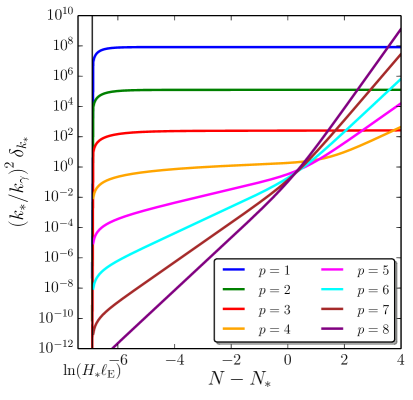
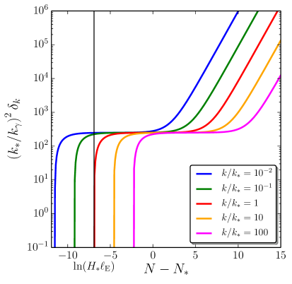
Figure 4: Decoherence parameter $\delta_{\bm{k}}$ [rescaled by $(k_{\gamma}/k_{*})^{2}$], computed with Eq. (4.5), as a function of time (labeled with the number of $e$-folds since Hubble exit of the pivot scale), for a few values of $p$ and a fixed value of $k=k_{*}$ (left panel) and for a few values of $k$ and a fixed value of $p=3$ (right panel). The values chosen for the other parameters are $\epsilon_{1*}=10^{-4}$, $\epsilon_{2*}=1-0.96-2\epsilon_{1*}$ and $H_{*}\ell_{\mathrm{E}}=10^{-3}$.

At linear order in $\gamma$, which is the order at which the Lindblad equation has been established in Appendix A, Eq. (4.2) gives rise to

$$\delta_{\bm{k}}(\eta) \simeq\left|v_{\bm{k}}^{\prime}\right|^{2}\mathcal{J}_{\bm{k}}+\left|v_{\bm{k}}\right|^{2}\mathcal{I}_{\bm{k}}-{\left|v_{\bm{k}}\right|^{2}}^{\prime}\mathcal{K}_{\bm{k}},$$ (4.4)

since one recalls that $\mathcal{I}_{\bm{k}}$, $\mathcal{J}_{\bm{k}}$ and $\mathcal{K}_{\bm{k}}$ all carry a factor $\gamma$, see Eqs. (3.8)-(3.10). As shown in Appendix C.2, the integrals $\mathcal{I}_{\bm{k}}$, $\mathcal{J}_{\bm{k}}$ and $\mathcal{K}_{\bm{k}}$ can be related to the quantities $I_{1}$ and $I_{2}$ defined in Eq. (C.29), see Eqs. (C.2)-(C.2). Plugging Eqs. (C.2)-(C.2) into Eq. (4.4), many cancellations occur (the reason behind all these cancellations will be made explicit in Sec. 4.1.5) and the following expression is obtained

$$\delta_{\bm{k}}\left(\eta\right)= \frac{\pi}{8\sin^{2}\left(\pi\nu\right)}\left(\frac{k_{\gamma}}{k_{*}}\right)^{2}\left(\frac{k}{k_{*}}\right)^{\left(p-3\right)\left(1+\epsilon_{1*}\right)-2}\left[I_{1}\left(\nu\right)+I_{1}\left(-\nu\right)-2\cos\left(\pi\nu\right)I_{2}\left(\nu\right)\right]\,.$$ (4.5)

The corresponding time evolution of $\delta_{\bm{k}}$ is displayed on the left panel of Fig. 4 for different values of $p$ and a fixed value of $k$ ($k=k_{*}$), and on the right panel for a fixed value of $p$ ($p=3$) and different values of $k$. On the left panel, one can see that $\delta_{\bm{k}}$ takes off very rapidly as soon as the mode under consideration crosses out the correlation length of the environment, and either settles to a stationary value afterwards (if $p\leq 2$) or continues to grow (if $p>2$). The case $p=3$ for different values of $k$ is displayed on the right panel, where one can see that after crossing out the environment correlation length, $\delta_{\bm{k}}$ remains stationary for some transient period of time and starts to increase again after a few $e$-folds. Since $\delta_{\bm{k}}$ always increases and since it takes off later for smaller scales (larger values of $k$), it is larger on larger scales (smaller values of $k$).

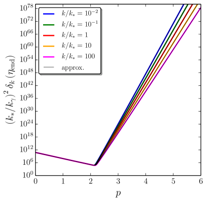
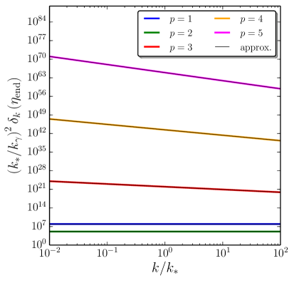
Figure 5: Decoherence parameter $\delta_{\bm{k}}$ [rescaled by $(k_{\gamma}/k_{*})^{2}$] at the end of inflation, as a function of $p$ and for a few values of $k$ (left panel) and as a function of $k$ for a few values of $p$ (right panel). The values chosen for the parameters are $\epsilon_{1*}=10^{-4}$, $\epsilon_{2*}=1-0.96-2\epsilon_{1*}$ and $H_{*}\ell_{\mathrm{E}}=10^{-3}$. The coloured lines correspond to the exact formula (4.5) while the black lines stand for the analytical approximation (4.6) (they are hard to distinguish because of the perfect matching).

This behaviour can be analytically understood by computing $\delta_{\bm{k}}$ at the end of inflation, when the modes of astrophysical interest today are well outside the Hubble radius and Eq. (4.5) can be expanded in the limit $-k\eta\ll 1$. Further assuming that $\ell_{\mathrm{E}}\ll H_{*}^{-1}$ (which was necessary to derive the Lindblad equation in Appendix A, at least if $\ell_{\mathrm{E}}\sim t_{\mathrm{c}}$), one obtains

$$\delta_{\bm{k}}(N)\simeq \frac{1}{4}\left(\frac{k_{\gamma}}{k_{*}}\right)^{2}\Biggl{\{}\frac{\left(H_{*}\ell_{\mathrm{E}}\right)^{\left(p-3\right)\left(1+\epsilon_{1*}\right)-1}}{1-\left(p-3\right)\left(1+\epsilon_{1*}\right)}\left(\frac{k}{k_{*}}\right)^{\left(p-3\right)\left(1+\epsilon_{1*}\right)-2}$$ (4.6)

$$-\frac{\Gamma^{2}\left(\nu\right)e^{\left(p-3-2\frac{1-\nu}{1+\epsilon_{1*}}\right)(N-N_{*})}}{2^{1-2\nu}\pi\left[2\left(1-\nu\right)-\left(p-3\right)\left(1+\epsilon_{1*}\right)\right]}\left(\frac{k}{k_{*}}\right)^{-2\nu}\Biggr{\}}\,.$$

In this equation, one can see that if the coefficient in the argument of the exponential is positive, namely $p>3+2(1-\nu)/(1+\epsilon_{1})$ (or, if one neglects slow-roll corrections, $p\gtrsim 2$), then $\delta_{\bm{k}}$ grows on large scales. If, on the contrary, $p\lesssim 2$, then the exponential becomes very quickly negligible and one is left with the first term, which is constant. This is agreement with the above discussion about Fig. 4.

In Fig. 5, we have represented $\delta_{\bm{k}}$ calculated at the end of inflation using the exact result (4.5) and the analytical approximation (4.6). In the left panel, $\delta_{\bm{k}}(\eta_{\mathrm{end}})$ is plotted as a function of $p$ and for a few values of $k$, and in the right panel it is plotted as a function of $k$ and for a few values of $p$. The coloured lines correspond to the exact result (4.5) while the black lines stand for the analytical approximation (4.6). Evidently, they match very well (and are in fact hard to distinguish).

Since decoherence at observable scales is characterised by the condition $\delta_{\bm{k}_{*}}\gg 1$, Eq. (4.6) allows us to calculate the minimum interaction strength that is required for decoherence to complete before the end of inflation. One obtains that decoherence occurs when

$$\frac{k_{\gamma}}{k_{*}}\gg\begin{cases}(H_{*}\ell_{\mathrm{E}})^{\frac{1-\left(p-3\right)\left(1+\epsilon_{1*}\right)}{2}}\quad&\mathrm{if}\quad p<3+\frac{2-2\nu}{1+\epsilon_{1*}}\,,\\ e^{\left(\frac{1-\nu}{1+\epsilon_{1*}}-\frac{p-3}{2}\right)\Delta N_{*}}\quad&\mathrm{if}\quad p>3+\frac{2-2\nu}{1+\epsilon_{1*}}\,.\end{cases}$$ (4.7)

4.1.3 Combining with observational constraints

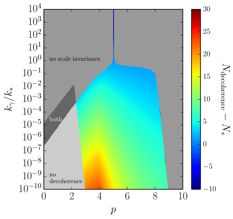
Figure 6: Regions in parameter space $(p,k_{\gamma}/k_{*})$ where decoherence and quasi scale invariance can or cannot be realised. The light grey region corresponds to values of $p$ and $k_{\gamma}/k_{*}$ where the interaction strength with the environment, parametrised by $k_{\gamma}/k_{*}$, see Eq. (3.4), is too small to lead to decoherence. The medium grey region is where it is too large to preserve quasi scale invariance, and the dark grey region is where both problems occur (no decoherence and scale invariance breaking). The coloured region corresponds to parameters where perturbations decohere and scale invariance is preserved. The colour code, indicated by the vertical bar, quantifies how many $e$-folds since Hubble crossing it takes before complete decoherence is reached. Here, decoherence is characterised by the condition $\delta_{\bm{k}_{*}}>10$, and quasi scale invariance by the condition $|n_{\scriptscriptstyle{\mathrm{S}}}-\bar{n}_{{}_{\mathrm{S}}}|<5\sigma_{n_{\scriptscriptstyle{\mathrm{S}}}}$, where $\bar{n}_{{}_{\mathrm{S}}}\simeq 0.96$ and $\sigma_{n_{\scriptscriptstyle{\mathrm{S}}}}\simeq 0.006$ are the mean value and standard deviation of the Planck spectral index measurement [70] respectively. The spectral index and the decoherence parameter are computed numerically without approximations.

We have shown that decoherence occurs in the presence of linear interactions with an environment if the interaction strength is sufficiently large and satisfies Eq. (4.7). However, in Sec. 3.1.6, it was explained that if the interaction strength is too large, quasi scale invariance is lost, which is observationally excluded. The upper bounds (3.39)-(3.41) on the interaction strength were then obtained. When the lower bound provided by Eq. (4.7) is smaller than the upper bound from Eqs. (3.39)-(3.41), there is a range of values for the interaction strength such that decoherence is obtained without spoiling scale invariance. This range is given by

$$e^{-\frac{\Delta N_{*}}{2}\left(p-2+\epsilon_{1*}+\epsilon_{2*}\right)}\ll\frac{k_{\gamma}}{k_{*}}\ll\begin{cases}\left(H_{*}\ell_{\mathrm{E}}\right)^{\frac{4-p}{2}}\ &\mathrm{if}\quad 2-\epsilon_{1*}-\epsilon_{2*}<p<4-\epsilon_{1*}\,,\\ 1\ &\mathrm{if}\quad 4-\epsilon_{1*}<p<8-3\epsilon_{1*}+\epsilon_{2*}\,,\\ e^{-\frac{\Delta N_{*}}{2}\left(p-8+3\epsilon_{1*}-\epsilon_{2*}\right)}\ &\mathrm{if}\quad 8-3\epsilon_{1*}+\epsilon_{2*}<p\,.\end{cases}$$ (4.8)

In particular, one can see that when $p<3+(2-2\nu)/(1+\epsilon_{1*})\simeq 2$, decoherence and quasi scale invariance cannot be achieved simultaneously, since Eq. (3.41) and the first of Eq. (4.7) directly contradict each other. This is because, from Eqs. (3.27) and (4.6), one can see that $\Delta\mathcal{P}_{\bm{k}}=2\delta_{\bm{k}}$ in that case.

This allows one to understand Fig. 6 where the situation is summarised. This figure represents the regions in parameter space $(p,k_{\gamma}/k_{*})$ where quasi scale invariance and decoherence can or cannot be realised. The light grey region corresponds to situations where the interaction strength with the environment is too small to yield decoherence. The medium grey region is where it is too large to preserve quasi scale invariance, and the dark grey region is where both problems occur (no decoherence and scale invariance breaking). For $p\lesssim 2$, one can see that decoherence cannot be realised without spoiling the quasi scale invariance of the power spectrum, in agreement with the above discussion. For $p\gtrsim 2$, there are intermediate values of $k_{\gamma}/k_{*}$ for which decoherence is obtained while preserving quasi scale invariance. This region is coloured in Fig. 6, and the colour code quantifies how many $e$-folds since Hubble crossing are needed in order to complete decoherence. One can check that the larger the interaction strength, the fewer $e$-folds it takes to reach decoherence. In general, decoherence happens after Hubble crossing (light blue to red regions), but it can also occur soon after crossing out the environment correlation length and before crossing out the Hubble radius (dark blue regions).

The most striking feature of the plot is probably the thin vertical line centred at $p=5$. As shown in Sec. 3.1.7, the origin of this line is the fact that for $p=5$, the correction to the power spectrum caused by the Lindblad term is itself scale invariant. As a consequence, even a very large value of the coupling constant can lead to quasi scale invariance. Let us also recall that $p\simeq 5$ is precisely the case that corresponds to the model described in Appendix B where inflationary perturbations couple to heavy scalar degrees of freedom. Fig. 6 highlights again the remarkable property of this type of environment, which allows cosmological perturbations to decohere during inflation without spoiling their scale invariance.

4.1.4 Can we neglect the free Hamiltonian?

It is sometimes argued that decoherence can be estimated without taking the free Hamiltonian into account, since no decoherence occurs in the free theory. In principle, this is true only if decoherence is so rapid that the free evolution of the system can be neglected while it occurs. Here we re-calculate the decoherence parameter in the absence of free evolution in order to determine when this is indeed the case.

Neglecting the free Hamiltonian terms in Eq. (3.6), one has

$$\frac{\mathrm{d}\left\langle v^{s,(1)}_{\bm{k}}\right|\hat{\rho}_{\bm{k}}^{s}\left|v^{s,(2)}_{\bm{k}}\right\rangle}{\mathrm{d}\eta} =-\frac{\gamma}{2}\left(2\pi\right)^{3/2}\tilde{C}_{R}({\bm{k}})\left[{v^{s,(1)}_{\bm{k}}}-{v^{s,(2)}_{\bm{k}}}\right]^{2}\left\langle v^{s,(1)}_{\bm{k}}\right|\hat{\rho}^{s}_{\bm{k}}\left|v^{s,(2)}_{\bm{k}}\right\rangle\,.$$ (4.9)

Using the Bunch-Davies vacuum as the initial state, this can be readily integrated and gives rise to Eq. (4.1) if one replaces $\delta_{\bm{k}}$ with $\delta_{\bm{k}}^{\mathrm{no}\,\mathrm{free}}$, defined as

$$\delta_{\bm{k}}^{\mathrm{no}\,\mathrm{free}}(\eta)=\left(2\pi\right)^{3/2}P_{vv}(k)\int_{-\infty}^{\eta}\gamma\left(\eta^{\prime}\right)\tilde{C}_{R}\left(\bm{k},\eta^{\prime}\right)\mathrm{d}\eta^{\prime}\,.$$ (4.10)

In this expression, $P_{vv}=|v_{\bm{k}}|^{2}+\mathcal{J}_{\bm{k}}$, see Eq. (3.13). Since $\mathcal{J}_{\bm{k}}$ is proportional to $\gamma$, it only adds terms of second order in $\gamma$ in Eq. (4.10), so if one wants to calculate $\delta_{\bm{k}}^{\mathrm{no}\,\mathrm{free}}$ at leading order in $\gamma$, it is enough to keep only the standard contribution to the power spectrum. Expanding $|v_{\bm{k}}|^{2}$ given by Eq. (C.24) in the super-Hubble limit, and making use of Eqs. (2.27) and (C.25), this gives rise to

$$\delta_{\bm{k}}^{\mathrm{no}\,\mathrm{free}}(N)\simeq \frac{1}{4}\left(\frac{k_{\gamma}}{k_{*}}\right)^{2}\Biggl{\{}\frac{\Gamma^{2}(\nu)\left(H\ell_{\mathrm{E}}\right)^{\left(p-3\right)\left(1+\epsilon_{1*}\right)-1}}{2^{1-2\nu}\pi[1-(p-3)(1+\epsilon_{1})]}\left(\frac{k}{k_{*}}\right)^{\left(p-3\right)\left(1+\epsilon_{1*}\right)-1-2\nu}e^{\frac{2\nu-1}{1+\epsilon_{1*}}\left(N-N_{*}\right)}$$ (4.11)

$$-\frac{\Gamma^{2}(\nu)e^{\left(p-3-2\frac{1-\nu}{1+\epsilon_{1*}}\right)(N-N_{*})}}{2^{1-2\nu}\pi[1-(p-3)(1+\epsilon_{1*})]}\left(\frac{k}{k_{*}}\right)^{-2\nu}\Biggr{\}}\,.$$

This expression needs to be compared with Eq. (4.6). Like Eq. (4.6), it is made of two terms and which one dominates at late time depends on the value of $p$. By comparing the exponentials of each term, one finds that if $p<3+1/(1+\epsilon_{1*})\simeq 4$, the first term dominates. In Eq. (4.6), the dominant term depends on whether $p$ is smaller or larger than $3+2(1-\nu)/(1+\epsilon_{1*})\simeq 2$ but since neither term matches the first term of Eq. (4.11), the two expressions strongly disagree in that case. If $p>3+1/(1+\epsilon_{1*})\simeq 4$, however, the second term in Eq. (4.11) dominates, which matches the second term of Eq. (4.6), up to a factor $\left[\left(p-3\right)\left(1+\epsilon_{1*}\right)-1\right]/\left[\left(p-3\right)\left(1+\epsilon_{1*}\right)-2\left(1-\nu\right)\right]$ that is of order one, and the two expressions agree in that case. Interestingly, $p=3+1/(1+\epsilon_{1*})$ corresponds to the limiting value between cases 2 and 3 in the classification introduced in Sec. 3.1.5, where it was shown that $p>3+1/(1+\epsilon_{1*})$ is the condition for the power spectrum to be independent of the environment correlation shape and length. We conclude that only in this case can the free Hamiltonian be neglected when computing the decoherence parameter. Further insight into this result is provided at the end of Sec. 4.1.5.

4.1.5 Alternative derivation of the decoherence parameter

Before moving on to study decoherence in the presence of quadratic interactions, let us show how the above result can be obtained without solving for the Lindblad equation (2.16) entirely. Indeed, in the case of quadratic interactions, a full solution to Eq. (2.16) is not available and we will need an alternative technique.

The starting point is to use Eq. (4.3), $\mathrm{Tr}(\hat{\rho}_{\bm{k}}^{s}{}^{2})=(1+4\delta_{\bm{k}})^{-1/2}$, as a definition of the decoherence parameter $\delta_{\bm{k}}$. Let us recall that when the state is pure, $\hat{\rho}_{\bm{k}}^{s}{}^{2}=\hat{\rho}_{\bm{k}}^{s}$ such that $\mathrm{Tr}(\hat{\rho}_{\bm{k}}^{s}{}^{2})=1$ and $\delta_{\bm{k}}=0$, while in the presence of decoherence, $\delta_{\bm{k}}>0$ and $\mathrm{Tr}(\hat{\rho}_{\bm{k}}^{s}{}^{2})<1$. Using the linearity and the cyclicity of the trace operator, one has

$$\frac{\mathrm{d}}{\mathrm{d}\eta}\mathrm{Tr}\left(\hat{\rho}_{\bm{k}}^{s}{}^{2}\right) =2\mathrm{Tr}\left(\hat{\rho}_{\bm{k}}^{s}\frac{\mathrm{d}\hat{\rho}_{\bm{k}}^{s}}{\mathrm{d}\eta}\right)$$ (4.12)

$$=-2i\mathrm{Tr}\left(\hat{\rho}_{\bm{k}}^{s}\left[\hat{\mathcal{H}}_{\bm{k}}^{s},\hat{\rho}_{\bm{k}}^{s}\right]\right)-\gamma(2\pi)^{3/2}\tilde{C}_{R}({\bm{k}})\mathrm{Tr}\left(\hat{\rho}_{\bm{k}}^{s}\left[\hat{v}_{\bm{k}}^{s},\left[\hat{v}_{\bm{k}}^{s},\hat{\rho}_{\bm{k}}^{s}\right]\right]\right)\,,$$

where in the second equality, the Lindblad equation (3.3) written in Fourier subspaces has been used. In this expression, using the cyclicity of the trace operator, one finds that the first term vanishes and the second one can be written as $\mathrm{Tr}(\hat{\rho}_{\bm{k}}^{s}[\hat{v}_{\bm{k}}^{s},[\hat{v}_{\bm{k}}^{s},\hat{\rho}_{\bm{k}}^{s}]])=2\mathrm{Tr}(\hat{\rho}_{\bm{k}}^{s}[\hat{\rho}_{\bm{k}}^{s},\hat{v}_{\bm{k}}^{s}]\hat{v}_{\bm{k}}^{s})$, so that Eq. (4.12) becomes

$$\frac{\mathrm{d}}{\mathrm{d}\eta}\mathrm{Tr}\left(\hat{\rho}_{\bm{k}}^{s}{}^{2}\right)=-2\gamma(2\pi)^{3/2}\tilde{C}_{R}({\bm{k}})\mathrm{Tr}\left(\hat{\rho}_{\bm{k}}^{s}\left[\hat{\rho}_{\bm{k}}^{s},\hat{v}_{\bm{k}}^{s}\right]\hat{v}_{\bm{k}}^{s}\right)$$ (4.13)

$$\qquad=-2\gamma(2\pi)^{3/2}\tilde{C}_{R}({\bm{k}})\int\mathrm{d}v_{\bm{k}}^{s,(1)}\int\mathrm{d}v_{\bm{k}}^{s,(2)}v_{\bm{k}}^{s,(1)}\left[v_{\bm{k}}^{s,(1)}-v_{\bm{k}}^{s,(2)}\right]\left|\left\langle v_{\bm{k}}^{s,(1)}\right|\hat{\rho}_{\bm{k}}^{s}\left|v_{\bm{k}}^{s,(2)}\right\rangle\right|^{2}\,,$$

where in the second equality, $\mathrm{Tr}(\hat{\rho}_{\bm{k}}^{s}[\hat{\rho}_{\bm{k}}^{s},\hat{v}_{\bm{k}}^{s}]\hat{v}_{\bm{k}}^{s})$ has been written explicitly in terms of the elements of the density matrix $\hat{\rho}_{\bm{k}}^{s}$.

The next step is to notice that at linear order in $\gamma$, it is enough to evaluate the right-hand side of the above equation in the free theory, where the density matrix is given by Eq. (3.11). In this case, the integrals appearing in Eq. (4.13) are Gaussian and can be performed explicitly, and one obtains $\mathrm{Tr}(\hat{\rho}_{\bm{k}}^{s}[\hat{\rho}_{\bm{k}}^{s},\hat{v}_{\bm{k}}^{s}]\hat{v}_{\bm{k}}^{s})=P_{vv}(k)$. The relation (4.13) can then be readily integrated, and expanding Eq. (4.3) at leading order in $\gamma$, $\mathrm{Tr}(\hat{\rho}_{\bm{k}}^{s}{}^{2})\simeq 1-2\delta_{\bm{k}}$, one obtains

$$\delta_{\bm{k}}\left(\eta\right) =\left(2\pi\right)^{3/2}\int_{-\infty}^{\eta}\gamma\left(\eta^{\prime}\right)\tilde{C}_{R}\left(k,\eta^{\prime}\right)P_{vv}\left(k,\eta^{\prime}\right)\mathrm{d}\eta^{\prime}$$ (4.14)

$$=\frac{1}{2}\int_{-\infty}^{\eta}S_{1}\left(\bm{k},\eta^{\prime}\right)P_{vv}\left(\bm{k},\eta^{\prime}\right)\mathrm{d}\eta^{\prime}\,,$$

where in the second line we have recast the result in terms of the source function $S_{1}$ defined in Eq. (3.22). Several remarks about this expression are in order.

First, let us notice that Eq. (4.14) is valid beyond the linear expansion in $\gamma$. Indeed, if one uses the exact solution (LABEL:eq:finalrhomaintext) to the Lindblad equation to calculate the integrals appearing in the right-hand side of Eq. (4.13), one obtains $\mathrm{Tr}(\hat{\rho}_{\bm{k}}^{s}[\hat{\rho}_{\bm{k}}^{s},\hat{v}_{\bm{k}}^{s}]\hat{\rho}_{\bm{k}}^{s})=P_{vv}(k)(1+4\delta_{\bm{k}})^{-3/2}=P_{vv}(k)\mathrm{Tr}^{3}(\hat{\rho}_{\bm{k}}^{s}{}^{2})$. This allows one to write Eq. (4.13) as a linear differential equation for $\mathrm{Tr}(\hat{\rho}_{\bm{k}}^{s}{}^{2})$, the solution of which gives rise to Eq. (4.14) when combined with Eq. (4.3). The formula (4.14) is therefore exact.

Second, at linear order in $\gamma$, the right-hand side of Eq. (4.14) can be evaluated in the free theory where $P_{vv}=|v_{\bm{k}}|^{2}$, where the mode function $v_{\bm{k}}$ is given by Eq. (C.24) in terms of Bessel functions. Making use of Eqs. (2.27) and (C.25), one obtains Eq. (4.5). This elucidates the numerous cancellations that appeared when going from Eq. (4.4) to Eq. (4.5), and which result from the equivalence between Eq. (4.4) and Eq. (4.14). In fact, without expanding in $\gamma$, the right-hand side of Eq. (4.14) can be evaluated with $P_{vv}=|v_{\bm{k}}|^{2}+\mathcal{J}_{\bm{k}}$, see Eq. (3.13), and this gives rise to Eq. (4.2). This explains why, since $P_{vv}$ is linear in $\gamma$, $\delta_{\bm{k}}$ is quadratic in $\gamma$.

Third, it is interesting to compare Eq. (4.14) with Eq. (4.10), which was obtained by neglecting the influence of the free Hamiltonian. One can see that the only difference between these two expressions is that in Eq. (4.10), the power spectrum is taken out of the integral and evaluated at the time $\eta$. This explains why only the contribution from the upper bound of the integral of Eq. (4.10) is correctly computed, up to a prefactor of order one.

4.2 Quadratic interaction

Let us now study decoherence as produced by quadratic interactions with an environment. As already explained, because of mode coupling, the Lindblad equation (2.16) does not decouple into a set of independent Lindblad equations for each Fourier mode, and cannot be solved entirely. This means that the calculation of Sec. 4.1.2 cannot be reproduced here, and that the alternative technique presented in Sec. 4.1.5 must instead be employed. Since the state is not factorisable into Fourier subspaces in the presence of quadratic interactions, i.e. Eq. (2.7) does not apply, the effective density matrix on the space $\left\{s\atop{\bm{k}}\right\}$ has first to be defined by tracing over all other degrees of freedom,

$$\hat{\rho}_{\bm{k}}^{s}\equiv\mathrm{Tr}_{\left\{s^{\prime}\atop{\bm{k}^{\prime}\neq\bm{k}}\right\},\left\{\bar{s}\atop{\bm{k}}\right\}}\left(\hat{\rho}_{v}\right)\,,$$ (4.15)

where $\bar{s}=\mathrm{I}$ if $s=\mathrm{R}$ and $\bar{s}=\mathrm{R}$ if $s=\mathrm{I}$. The decoherence parameter $\delta_{\bm{k}}$ is then defined according to Eq. (4.3) through $\mathrm{Tr}_{\left\{s\atop{\bm{k}}\right\}}(\hat{\rho}_{\bm{k}}^{s}{}^{2})$.

4.2.1 Decoherence criterion

Making use of the linearity and ciclycity of the trace operator, one has

$$\frac{\mathrm{d}}{\mathrm{d}\eta}\mathrm{Tr}_{\left\{s\atop{\bm{k}}\right\}}\left(\hat{\rho}_{\bm{k}}^{s}{}^{2}\right) =2\mathrm{Tr}_{\left\{s\atop{\bm{k}}\right\}}\left[\mathrm{Tr}_{\left\{s^{\prime}\atop{\bm{k}^{\prime}\neq\bm{k}}\right\},\left\{\bar{s}\atop{\bm{k}}\right\}}\left(\hat{\rho}_{v}\right)\frac{\mathrm{d}}{\mathrm{d}\eta}\mathrm{Tr}_{\left\{s^{\prime}\atop{\bm{k}^{\prime}\neq\bm{k}}\right\},\left\{\bar{s}\atop{\bm{k}}\right\}}\left(\hat{\rho}_{v}\right)\right]$$ (4.16)

$$=2\mathrm{Tr}_{\left\{s\atop{\bm{k}}\right\}}\left[\hat{\rho}_{\bm{k}}^{s}\mathrm{Tr}_{\left\{s^{\prime}\atop{\bm{k}^{\prime}\neq\bm{k}}\right\},\left\{\bar{s}\atop{\bm{k}}\right\}}\left(\frac{\mathrm{d}\hat{\rho}_{v}}{\mathrm{d}\eta}\right)\right]\,.$$

In this expression, $\mathrm{d}\hat{\rho}_{v}/\mathrm{d}\eta$ needs to be replaced by the Lindblad equation (2.16) (with $\hat{A}=\hat{v}^{2}$), which contains two terms. The first one involves the free Hamiltonian (2.1) and is, in practice, difficult to incorporate in the following calculation. However, the contribution from this term to the decoherence parameter only reflects the correlations that develop between the Fourier subspace $\left\{s\atop{\bm{k}}\right\}$ under consideration and the other Fourier subspaces, over which we have traced over, see Eq. (4.15). The reason for this partial trace is not that we do not “observe” the other Fourier degrees of freedom, but is because we want to define a decoherence parameter for each Fourier subspace, by analogy with the linear case. If the state were factorisable, the Hamiltonian contribution to Eq. (4.16) would vanish, which is why it is simply discarded in what follows. The second term coming from Eq. (2.16) is the Lindblad term. Fourier expanding $\hat{v}$ and $C_{R}$, it gives rise to

$$\mathrm{Tr}_{\left\{s^{\prime}\atop{\bm{k}^{\prime}\neq\bm{k}}\right\},\left\{\bar{s}\atop{\bm{k}}\right\}}\left(\frac{\mathrm{d}\hat{\rho}_{v}}{\mathrm{d}\eta}\right)= -\frac{\gamma}{2}\left(2\pi\right)^{-3/2}\int_{\mathbb{R}^{3}}\mathrm{d}\bm{k}_{1}\mathrm{d}\bm{k}_{2}\mathrm{d}\bm{k}_{3}\tilde{C}_{R}\left(\bm{k}_{1}\right)$$ (4.17)

$$\quad\mathrm{Tr}_{\left\{s^{\prime}\atop{\bm{k}^{\prime}\neq\bm{k}}\right\},\left\{\bar{s}\atop{\bm{k}}\right\}}\left(\left[\hat{v}_{\bm{k}_{2}}\hat{v}_{-\bm{k}_{1}-\bm{k}_{2}},\left[\hat{v}_{\bm{k}_{3}}\hat{v}_{\bm{k}_{1}-\bm{k}_{3}},\hat{\rho}_{v}\right]\right]\right)\,.$$

At leading order in $\gamma$, the second line of the above expression can be evaluated in the free theory, where the density matrix is factorisable and given by Eqs. (2.7) and (3.11).

Let us consider the case where $\bm{k}\notin\{\pm\bm{k}_{2},\pm(\bm{k}_{1}+\bm{k}_{2}),\pm\bm{k}_{3},\pm(\bm{k}_{1}-\bm{k}_{3})\}$. By removing $\hat{\rho}_{\bm{k}}^{s}$ from the trace in the second line of Eq. (4.16) (since it commutes with all $\hat{v}$ operators), one is left with a full (as opposed to partial) trace, that vanishes. This means that $\bm{k}$ must be equal, up to a sign (recall that $\bm{k}$ and $\bm{k}^{\prime}$ live in $\mathbb{R}^{3+}$ while $\bm{k}_{1}$, $\bm{k}_{2}$ and $\bm{k}_{3}$ live in $\mathbb{R}^{3}$), to one of the wavenumbers that index the $\hat{v}$ operators in Eq. (4.17). If it is equal to one such wavenumber only and the other three are different, one can show that the trace vanishes again, such that $\bm{k}$ must be equal to 2, 3 and all 4 wavenumbers that index the $\hat{v}$ operators in Eq. (4.17). Let us discuss these three possibilities separately.

We first examine the situation where $\bm{k}$ is equal to two of the wavenumbers that index the $\hat{v}$ operators in Eq. (4.17). For instance, let us consider the case where $\bm{k}=\bm{k}_{2}=-\bm{k}_{3}$ and $\bm{k}_{1}\neq-2\bm{k}$, for which one has

$$\kern-50.00008pt\mathrm{Tr}_{\left\{s^{\prime}\atop{\bm{k}^{\prime}\neq\bm{k}}\right\},\left\{\bar{s}\atop{\bm{k}}\right\}}\left(\left[\hat{v}_{\bm{k}}\hat{v}_{-\bm{k}_{1}-\bm{k}},\left[\hat{v}_{-\bm{k}}\hat{v}_{\bm{k}_{1}+\bm{k}},\hat{\rho}_{v}\right]\right]\right)=$$ (4.18)

$$\mathrm{Tr}_{\left\{\bar{s}\atop{\bm{k}}\right\}}\left(\hat{v}_{\bm{k}}\hat{v}_{-\bm{k}}\hat{\rho}_{\bm{k}}^{s}\hat{\rho}_{\bm{k}}^{\bar{s}}\right)\mathrm{Tr}_{\left\{s,\bar{s}\atop{\bm{k}+\bm{k}_{1}}\right\}}\left(\hat{v}_{-\bm{k}-\bm{k}_{1}}\hat{v}_{\bm{k}+\bm{k_{1}}}\hat{\rho}_{\bm{k}+\bm{k_{1}}}^{s}\rho_{\bm{k}+\bm{k_{1}}}^{\bar{s}}\right)$$

$$- \mathrm{Tr}_{\left\{\bar{s}\atop{\bm{k}}\right\}}\left(\hat{v}_{\bm{k}}\hat{\rho}_{\bm{k}}^{s}\hat{\rho}_{\bm{k}}^{\bar{s}}\hat{v}_{-\bm{k}}\right)\mathrm{Tr}_{\left\{s,\bar{s}\atop{\bm{k}+\bm{k}_{1}}\right\}}\left(\hat{v}_{-\bm{k}-\bm{k}_{1}}\hat{\rho}_{\bm{k}+\bm{k_{1}}}^{s}\rho_{\bm{k}+\bm{k_{1}}}^{\bar{s}}\hat{v}_{\bm{k}+\bm{k_{1}}}\right)$$

$$- \mathrm{Tr}_{\left\{\bar{s}\atop{\bm{k}}\right\}}\left(\hat{v}_{-\bm{k}}\hat{\rho}_{\bm{k}}^{s}\hat{\rho}_{\bm{k}}^{\bar{s}}\hat{v}_{\bm{k}}\right)\mathrm{Tr}_{\left\{s,\bar{s}\atop{\bm{k}+\bm{k}_{1}}\right\}}\left(\hat{v}_{\bm{k}+\bm{k}_{1}}\hat{\rho}_{\bm{k}+\bm{k_{1}}}^{s}\rho_{\bm{k}+\bm{k_{1}}}^{\bar{s}}\hat{v}_{-\bm{k}-\bm{k_{1}}}\right)$$

$$+ \mathrm{Tr}_{\left\{\bar{s}\atop{\bm{k}}\right\}}\left(\hat{\rho}_{\bm{k}}^{s}\hat{\rho}_{\bm{k}}^{\bar{s}}\hat{v}_{-\bm{k}}\hat{v}_{\bm{k}}\right)\mathrm{Tr}_{\left\{s,\bar{s}\atop{\bm{k}+\bm{k}_{1}}\right\}}\left(\hat{\rho}_{\bm{k}+\bm{k_{1}}}^{s}\rho_{\bm{k}+\bm{k_{1}}}^{\bar{s}}\hat{v}_{\bm{k}+\bm{k}_{1}}\hat{v}_{-\bm{k}-\bm{k_{1}}}\right)$$

$$= \frac{1}{2}\left[\hat{v}_{\bm{k}}^{s},\left[\hat{v}_{\bm{k}}^{s},\hat{\rho}_{\bm{k}}^{s}\right]\right]P_{vv}\left({\bm{k}}+{\bm{k}}_{1}\right)\,,$$

where we have used the decomposition $\hat{v}_{\bm{k}}=(\hat{v}_{\bm{k}}^{\mathrm{R}}+i\hat{v}_{\bm{k}}^{\mathrm{I}})/\mathchoice{{\hbox{$\displaystyle\sqrt{2\,}$}\lower 0.4pt\hbox{\vrule height=6.44444pt,depth=-5.15558pt}}}{{\hbox{$\textstyle\sqrt{2\,}$}\lower 0.4pt\hbox{\vrule height=6.44444pt,depth=-5.15558pt}}}{{\hbox{$\scriptstyle\sqrt{2\,}$}\lower 0.4pt\hbox{\vrule height=4.51111pt,depth=-3.6089pt}}}{{\hbox{$\scriptscriptstyle\sqrt{2\,}$}\lower 0.4pt\hbox{\vrule height=3.22221pt,depth=-2.57779pt}}}$. The same result is obtained with $\bm{k}=\bm{k}_{2}=\bm{k}_{3}-\bm{k}_{1}$, $\bm{k}=-\bm{k}_{1}-\bm{k_{2}}=-\bm{k}_{3}$ or $\bm{k}=-\bm{k}_{1}-\bm{k_{2}}=-\bm{k}_{1}+\bm{k_{3}}$, if the condition $\bm{k}_{1}\neq-2\bm{k}$ is enforced. In the same manner, if $\bm{k}=-\bm{k}_{2}=\bm{k}_{3}$, $\bm{k}=-\bm{k}_{2}=\bm{k}_{1}-\bm{k}_{3}$, $\bm{k}=\bm{k}_{1}+\bm{k}_{2}=\bm{k}_{3}$ or $\bm{k}=\bm{k}_{1}+\bm{k}_{2}=\bm{k}_{1}-\bm{k}_{3}$, and if the condition $\bm{k}_{1}\neq 2\bm{k}$ is enforced, the same result as in Eq. (4.18) is obtained, except that the power spectrum is evaluated at $\bm{k}-\bm{k}_{1}$ instead of $\bm{k}+\bm{k}_{1}$. One can check that all other configurations give a vanishing result.

Then, one can show that the case where $\bm{k}$ is equal to three of the wavenumbers that index the $\hat{v}$ operators in Eq. (4.17) gives contributions that are always proportional to the quantum mean value of a single mode function operator and therefore vanish, see the discussion below Eq. (3.16). Finally remains the situation where all wavenumbers are, up a sign, equal. For instance, let us consider the case where $\bm{k_{1}}=-2\bm{k}$, $\bm{k}_{2}=\bm{k}$ and $\bm{k}_{3}=-\bm{k}$, for which one has

$$\mathrm{Tr}_{\left\{s^{\prime}\atop{\bm{k}^{\prime}\neq\bm{k}}\right\},\left\{\bar{s}\atop{\bm{k}}\right\}}\left(\left[\hat{v}_{\bm{k}}\hat{v}_{\bm{k}},\left[\hat{v}_{-\bm{k}}\hat{v}_{-\bm{k}},\hat{\rho}_{v}\right]\right]\right) =\mathrm{Tr}_{\left\{\bar{s}\atop{\bm{k}}\right\}}\left(\left[\hat{v}_{\bm{k}}\hat{v}_{\bm{k}},\left[\hat{v}_{-\bm{k}}\hat{v}_{-\bm{k}},\hat{\rho}_{\bm{k}}^{s}\hat{\rho}_{\bm{k}}^{\bar{s}}\right]\right]\right)$$ (4.19)

$$=\frac{1}{4}\left[\hat{v}_{\bm{k}}^{s}{}^{2},\left[\hat{v}_{\bm{k}}^{s}{}^{2},\hat{\rho}_{\bm{k}}^{s}\right]\right]+P_{vv}\left(\bm{k}\right)\left[\hat{v}_{\bm{k}}^{s},\left[\hat{v}_{\bm{k}}^{s},\hat{\rho}_{\bm{k}}^{s}\right]\right]\,.$$

The only other non-vanishing configuration of this type is when $\bm{k_{1}}=2\bm{k}$, $\bm{k}_{2}=-\bm{k}$ and $\bm{k}_{3}=\bm{k}$, which gives the same result. These contributions are however suppressed by a volume factor with respect to the ones giving Eq. (4.18), since they do not vanish only for a single configuration of the wavenumbers $\bm{k}_{1}$, $\bm{k}_{2}$ and $\bm{k}_{3}$, while the configurations leading to Eq. (4.18) leave one wavenumber free. This is why, in the factorisable state, one obtains that

$$\kern-20.00003pt\mathrm{Tr}_{\left\{s^{\prime}\atop{\bm{k}^{\prime}\neq\bm{k}}\right\},\left\{\bar{s}\atop{\bm{k}}\right\}}\left(\left[\hat{v}_{\bm{k}_{2}}\hat{v}_{-\bm{k}_{1}-\bm{k}_{2}},\left[\hat{v}_{\bm{k}_{3}}\hat{v}_{\bm{k}_{1}-\bm{k}_{3}},\hat{\rho}_{v}\right]\right]\right)=\frac{1}{2}\left[\hat{v}_{\bm{k}}^{s},\left[\hat{v}_{\bm{k}}^{s},\hat{\rho}_{\bm{k}}^{s}\right]\right]\times$$ (4.20)

$$\Big{\{} P_{vv}\left({\bm{k}}+{\bm{k}}_{1}\right)\left[\delta\left({\bm{k}}_{2}-{\bm{k}}\right)+\delta\left({\bm{k}}_{2}+{\bm{k}}_{1}+{\bm{k}}\right)\right]\left[\delta\left({\bm{k}}_{3}+{\bm{k}}\right)+\delta\left({\bm{k}}_{3}-{\bm{k}}_{1}-{\bm{k}}\right)\right]$$

$$+ P_{vv}\left({\bm{k}}-{\bm{k}}_{1}\right)\left[\delta\left({\bm{k}}_{2}+{\bm{k}}\right)+\delta\left({\bm{k}}_{2}-{\bm{k}}_{1}+{\bm{k}}\right)\right]\left[\delta\left({\bm{k}}_{3}-{\bm{k}}\right)+\delta\left({\bm{k}}_{3}-{\bm{k}}_{1}+{\bm{k}}\right)\right]\Big{\}}\,.$$

Plugging back this expression into Eq. (4.17), the integrals over $\bm{k}_{2}$ and $\bm{k}_{3}$ can be performed, and one finds that the right-hand side of Eq. (4.17) is given by $-[\hat{v}_{\bm{k}}^{s},[\hat{v}_{\bm{k}}^{s},\hat{\rho}_{\bm{k}}^{s}]]S_{2}/4$, where $S_{2}$ is the source function defined in Eq. (3.53) and computed in Eq. (3.60). Inserting the result into Eq. (4.16), one obtains

$$\frac{\mathrm{d}}{\mathrm{d}\eta}\mathrm{Tr}_{\left\{s\atop{\bm{k}}\right\}}\left(\hat{\rho}_{\bm{k}}^{s}{}^{2}\right) =-S_{2}\left(\bm{k},\eta\right)\mathrm{Tr}_{\left\{s\atop{\bm{k}}\right\}}\left(\hat{\rho}_{\bm{k}}^{s}\left[\hat{v}_{\bm{k}}^{s},\left[\hat{v}_{\bm{k}}^{s},\hat{\rho}_{\bm{k}}^{s}\right]\right]\right)=-S_{2}\left(\bm{k},\eta\right)P_{vv}\left(\bm{k},\eta\right)\,,$$ (4.21)

where in the second equality we have used the formula $\mathrm{Tr}(\hat{\rho}_{\bm{k}}^{s}[\hat{v}_{\bm{k}}^{s},[\hat{v}_{\bm{k}}^{s},\hat{\rho}_{\bm{k}}^{s}]])=P_{vv}(k)$ derived around Eq. (4.13). At leading order in $\gamma$, $\mathrm{Tr}_{\left\{s\atop{\bm{k}}\right\}}\left(\hat{\rho}_{\bm{k}}^{s}{}^{2}\right)\simeq 1-2\delta_{\bm{k}}$, and this gives rise to

$$\delta_{\bm{k}}=\frac{1}{2}\int_{-\infty}^{\eta}S_{2}\left(\bm{k},\eta^{\prime}\right)P_{vv}\left(\bm{k},\eta^{\prime}\right)\mathrm{d}\eta^{\prime}\,.$$ (4.22)

which is analogous to Eq. (4.14). This suggests that the above formula is in fact generic, in the same way that Eq. (3.56) for the power spectrum applies for any source function.

4.2.2 Calculation of the decoherence parameter

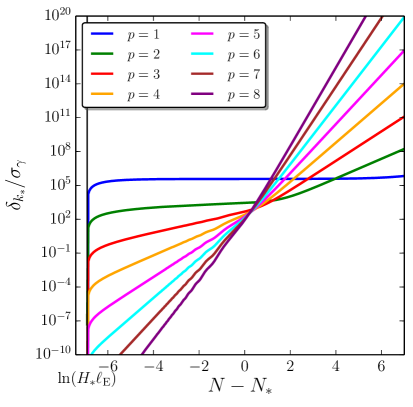
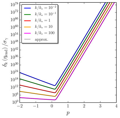
Figure 7: Left panel: decoherence parameter $\delta_{\bm{k}}$ (rescaled by $\sigma_{\gamma}$), computed with Eq. (4.23), as a function of time (labeled with the number of $e$-folds since Hubble exit of the pivot scale), for a few values of $p$ and a fixed value of $k=k_{*}$. Right panel: decoherence parameter at the end of inflation, as a function of $p$ and for a few values of $k$. The coloured lines correspond to the exact formula (4.23) while the black lines stand for the analytical approximation (4.24) (they are hard to distinguish because of the perfect matching). The values chosen for the parameters are $H_{*}\ell_{\mathrm{E}}=10^{-3}$, $\Delta N_{*}=50$, and $N_{{}_{\mathrm{T}}}=N_{\mathrm{end}}-N_{{}_{\mathrm{IR}}}=10^{4}$.

Since the calculation is being performed at linear order in $\gamma$, the right-hand side of Eq. (4.22) must be evaluated in the free theory where $P_{vv}=|v_{\bm{k}}|^{2}$, and the mode function $v_{\bm{k}}$ is given by Eq. (C.24). Making use of Eq. (3.60) for the source function with Eq. (2.27) for the environment correlator, one obtains

$$\delta_{\bm{k}}\left(\eta\right)=-\frac{\sigma_{\gamma}}{3\sin^{2}\left(\pi\nu\right)}\left(\frac{k_{*}}{k}\right)^{\alpha_{2}+1}\left[I_{3}\left(\nu\right)+I_{3}\left(-\nu\right)-2\cos\left(\pi\nu\right)I_{4}\left(\nu\right)\right]\,,$$ (4.23)

where $\sigma_{\gamma}$ has been defined in Eq. (3.64), $I_{3}$ and $I_{4}$ are defined in Appendix D.2 in Eq. (D.18), and where, neglecting slow-roll corrections for the reason given in Sec. 3.2.3, $\nu=3/2$ and $\alpha_{2}=2-p$. Let us notice that the structure of Eq. (4.23) is very similar to the corresponding expression in the case of linear interactions, namely Eq. (4.5).

The corresponding time evolution of $\delta_{\bm{k}}$ is displayed on the left panel of Fig. 7 for different values of $p$ and at the pivot scale $k_{*}$. The main difference with the case of linear interactions shown in Fig. 4 is that, here, $\delta_{\bm{k}}$ continues to increase at late time for all values of $p$ that are shown. This can be understood analytically by computing $\delta_{\bm{k}}$ close to the end of inflation, when the modes of astrophysical interest today are well outside the Hubble radius and Eq. (4.5) can be expanded in the limit $-k\eta\ll 1$. Further assuming that $\ell_{\mathrm{E}}\ll H_{*}^{-1}$, the integrals $I_{3}$ and $I_{4}$ can be expanded according to Eqs. (D.22) and (D.26) respectively, and one obtains

$$\delta_{\bm{k}}\left(N\right)\simeq\frac{2\sigma_{\gamma}}{3\pi} \left\{\left(\frac{k}{k_{*}}\right)^{-3}e^{p\left(N-N_{*}\right)}\frac{p\left(N-N_{{}_{\mathrm{IR}}}\right)-1}{p^{2}}\right.$$ (4.24)

$$\left.+\left(\frac{k}{k_{*}}\right)^{p-3}\frac{\left(H_{*}\ell_{\mathrm{E}}\right)^{p-2}}{2-p}\left[\frac{1}{2-p}+\ln\left(H_{*}\ell_{\mathrm{E}}\right)+\ln\left(\frac{k}{k_{*}}\right)+N_{{}_{\mathrm{T}}}-\Delta N_{*}\right]\right\}\,.$$

In the right panel of Fig. 7, we have represented $\delta_{\bm{k}}$ calculated at the end of inflation using the exact result (4.23) (coloured lines) and the analytical approximation (4.24) (black lines), and they match very well.

In Eq. (4.24), one can see that if $p>0$, the first term dominates at late time and $\delta_{\bm{k}}$ grows on large scales, in agreement with what can be seen on the left panel of Fig. 7. If, on the contrary, $p<0$, the exponential in the first term becomes very quickly negligible and one is left with the second term, which is constant. Recalling that decoherence at observable scales is characterised by the condition $\delta_{{\bm{k}}_{*}}\gg 1$, Eq. (4.24) allows us to calculate the minimum interaction strength that is required for decoherence to complete before the end of inflation,

$$\sigma_{\gamma}\gg\begin{cases}\dfrac{\left(H_{*}\ell_{\mathrm{E}}\right)^{2-p}}{\ln\left(H_{*}\ell_{\mathrm{E}}\right)+N_{{}_{\mathrm{T}}}-\Delta N_{*}}\quad&\mathrm{if}\quad p<0\,,\\ \dfrac{e^{-p\Delta N_{*}}}{N_{{}_{\mathrm{T}}}}\quad&\mathrm{if}\quad p>0\,.\end{cases}$$ (4.25)

4.2.3 Combining with observational constraints

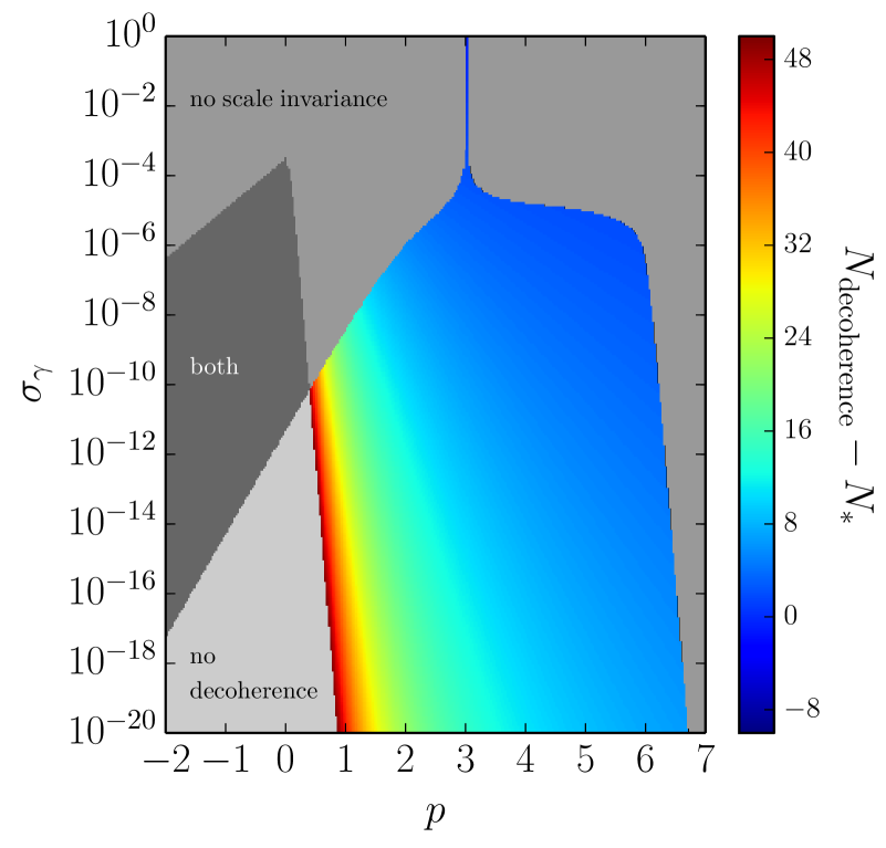
Figure 8: Regions in parameter space $(p,\sigma_{\gamma})$ where decoherence and quasi scale invariance can or cannot be realised. The light grey region corresponds to values of $p$ and $\sigma_{\gamma}$ where the interaction strength with the environment, parametrised by $\sigma_{\gamma}$, see Eq. (3.64), is too small to lead to decoherence. The medium grey region is where it is too large to preserve quasi scale invariance, and the dark grey region is where both problems occur (no decoherence and scale invariance breaking). The coloured region corresponds to parameters where perturbations decohere and scale invariance is preserved. The colour code, indicated by the vertical bar, quantifies how many $e$-folds since Hubble crossing it takes before complete decoherence is reached. This map is obtained with similar conventions as in Fig. 6.

As for the case of linear interactions, these lower bounds can be combined with the upper bounds derived in Sec. 3.2.4 from the requirement that the quasi scale invariance of the power spectrum is preserved. One obtains that the range of values for the interaction strength, here parametrised by $\sigma_{\gamma}$, such that decoherence occurs without spoiling scale invariance is given by

$${e^{-p\Delta N_{*}}}\ll N_{{}_{\mathrm{T}}}\sigma_{\gamma}\ll\begin{cases}{\left(H_{*}\ell_{\mathrm{E}}\right)^{2-p}}\quad&\mathrm{if}\quad 0<p<2\,,\\ 1\quad&\mathrm{if}\quad 2<p<6\,,\\ e^{\left(6-p\right)\Delta N_{*}}\quad&\mathrm{if}\quad p>6\,.\end{cases}$$ (4.26)

In particular, one can see that when $p<0$, the correction to the power spectrum given in Eq. (3.63) and the decoherence parameter given by the first line of Eq. (4.24) are directly related, $\left.\Delta{\cal P}_{\bm{k}}\right|_{3}=2\delta_{\bm{k}}$, which explains why decoherence cannot occur without spoiling the quasi scale invariance of the power spectrum.

The situation is summarised in Fig. 8, which represents the regions in parameter space where quasi scale invariance and decoherence can or cannot be realised. The conventions are the same as the ones used in Fig. 6 in the case of linear interactions, and all remarks made about that figure apply here too. As for linear interactions, the striking feature of Fig. 8 is the presence of a thin vertical line centred at $p=3$, for which the correction to the power spectrum caused by the Lindblad term is scale invariant, and observations do not constrain the interaction strength. Let us stress again that $p\simeq 3$ precisely corresponds to the model described in Appendix B where inflationary perturbations couple to heavy scalar degrees of freedom.

5 Generalisation to higher-order interactions

So far, we have shown that the effective inclusion of environmental degrees of freedom, through a Lindblad equation, gives rise to a modified power spectrum and to a decoherence parameter that can be calculated from a source function, see Eq. (3.56) and Eq. (4.22) respectively. In the case of linear interactions, $n=1$, the source function is given by Eq. (3.22), namely

$$S_{1}\left(\bm{k},\eta\right)=2(2\pi)^{3/2}\gamma\tilde{C}_{R}\left(k\right)\,.$$ (5.1)

For quadratic interactions, $n=2$, one can rewrite Eq. (3.53) as

$$S_{2}\left(\bm{k},\eta\right)=\frac{8\gamma}{(2\pi)^{3/2}}\int\mathrm{d}{\bm{p}}_{1}\,\tilde{C}_{R}\left({\bm{k}-\bm{p}}_{1}\right)P_{vv}\left(\bm{p}_{1}\right)\,,$$ (5.2)

where the power spectrum has to be evaluated in the free theory at leading order in $\gamma$. As explained in Sec. 3.2.3 (see also Appendix D.1), the convolution product between the power spectrum and the environment correlator, which appears in Eq. (5.2), is dominated by its IR contribution where $\bm{p}_{1}$ is super Hubble (if the UV contribution is not simply removed by adiabatic subtraction). Since the environment correlator $\tilde{C}_{R}$ selects out modes that have crossed out the environment correlation length $\ell_{\mathrm{E}}$, which is much smaller than the Hubble radius, the source function is well approximated by the environment correlator times the integrated power spectrum,

$$S_{2}\left(\bm{k},\eta\right)\simeq\frac{8\gamma}{(2\pi)^{3/2}}\tilde{C}_{R}\left({k}\right)\int_{p_{1}<aH}\mathrm{d}{\bm{p}}_{1}P_{vv}\left(p_{1}\right)\,.$$ (5.3)

Before concluding this work, let us try to generalise our approach to higher-order interaction terms. For instance, let us consider a cubic interaction, $\hat{A}=\hat{v}^{3}$. In that case, a long but straightforward calculation, similar to the one presented at the beginning of Sec. 3.2.1, gives the same system as in Eq. (3.48), except that the second line of the last entry now reads

$$-\frac{1}{2}\mathrm{Tr}\left\{\int\mathrm{d}\bm{x}\mathrm{d}\bm{y}C_{R}\left(\bm{x}-\bm{y}\right)\left[\left[\hat{p}_{\bm{k}_{1}}\hat{p}_{\bm{k}_{2}},\hat{v}^{3}\left(\bm{x}\right)\right],\hat{v}^{3}\left(\bm{y}\right)\right]\hat{\rho}_{v}\right\}$$ (5.4)

$$\qquad\qquad=\frac{9}{\left(2\pi\right)^{9/2}}\delta\left(\bm{k}_{1}+\bm{k}_{2}\right)\int\mathrm{d}\bm{p}_{1}\mathrm{d}\bm{p}_{2}\mathrm{d}\bm{p}_{3}\tilde{C}_{R}\left(\bm{p}_{1}+\bm{p}_{2}+\bm{k}_{1}\right)\mathcal{T}_{4}\left(\bm{p}_{1},\bm{p}_{2},\bm{p}_{3}\right)\,.$$

In this expression, the trispectrum has been defined according to $\langle\hat{v}_{\bm{p}_{1}}\hat{v}_{\bm{p}_{2}}\hat{v}_{\bm{p}_{3}}\hat{v}_{\bm{p}_{4}}\rangle=\mathcal{T}_{4}(\bm{p}_{1},\bm{p}_{2},\bm{p}_{3})\delta\left(\bm{p}_{1}+\bm{p}_{2}+\bm{p}_{3}+\bm{p}_{4}\right)$. One then obtains the differential equation (3.52) for the power spectrum, where the source function is given by $S_{3}$, which is such that the quantity written in Eq. (LABEL:eq:neq3:Ppp) equals $S_{3}(\bm{k}_{1})\delta(\bm{k}_{1}+\bm{k}_{2})/2$. At leading order in $\gamma$, it can be evaluated in the free theory where the state is Gaussian and one has $\left\langle\hat{v}_{\bm{p}_{1}}\hat{v}_{\bm{p}_{2}}\hat{v}_{{\bm{k}}_{3}}\hat{v}_{\bm{p}_{4}}\right\rangle=P_{vv}\left(p_{1}\right)P_{vv}\left(p_{3}\right)\delta(\bm{p}_{1}+\bm{p}_{2})\delta(\bm{p}_{3}+\bm{p}_{4})+P_{vv}\left(p_{1}\right)P_{vv}\left(p_{2}\right)\delta(\bm{p}_{1}+\bm{p}_{3})\delta(\bm{p}_{2}+\bm{p}_{4})+P_{vv}\left(p_{1}\right)P_{vv}\left(p_{2}\right)\delta(\bm{p}_{1}+\bm{p}_{4})\delta(\bm{p}_{2}+\bm{p}_{3})$ according to Wick theorem. This gives rise to

$$S_{3}\left(\bm{k},\eta\right)=\frac{18\gamma}{\left(2\pi\right)^{9/2}} \left[2\int\mathrm{d}\bm{p}_{1}\mathrm{d}\bm{p}_{2}\tilde{C}_{R}\left(\bm{k}-\bm{p}_{1}-\bm{p}_{2}\right)P_{vv}\left(\bm{p}_{1}\right)P_{vv}\left(\bm{p}_{2}\right)\right.$$ (5.5)

$$\left.+\tilde{C}_{R}\left(\bm{k}\right)\int\mathrm{d}\bm{p}_{1}\mathrm{d}\bm{p}_{2}P_{vv}\left(\bm{p}_{1}\right)P_{vv}\left(\bm{p}_{2}\right)\right]\,.$$

As for quadratic interactions, in the limit $\ell_{\mathrm{E}}\ll H^{-1}$ and keeping the IR component of these integrals only, this reduces to

$$S_{3}\left(\bm{k},\eta\right)\simeq\frac{54\gamma}{\left(2\pi\right)^{9/2}}\tilde{C}_{R}\left(k\right)\left[\int\mathrm{d}\bm{p}P_{vv}\left(\bm{p}\right)\right]^{2}\,.$$ (5.6)

Figure 9: Feynman diagrams representation of the source function. Straight and wiggly lines stand for propagators of the Mukhanov-Sasaki variable $\hat{v}$, and of the environment operator $\hat{R}$ it couples to, respectively. The first diagram corresponds to linear interactions $\propto\hat{v}\hat{R}$, and the second diagram is for quadratic interactions $\propto\hat{v}^{2}\hat{R}$.

5.1 Diagrammatic calculation of the source

The formulas obtained for the source function for linear interactions in Eq. (5.1), for quadratic interactions in Eq. (5.2), and now for cubic interactions in Eq. (5.5), can be understood with the diagrammatic representation shown in Figs. 9 and 10. In these Feynman diagrams, straight and wiggly lines represent propagators of the Mukhanov-Sasaki variable $\hat{v}$, and of the environment operator $\hat{R}$ it couples to, respectively.

The first diagram in Fig. 9 stands for linear interactions of the form $\hat{v}\hat{R}$. This is why one straight line and one wiggly line are attached to each vertex. Momentum conservation imposes that $\bm{k}_{1}=-\bm{k}_{2}=\bm{k}$ and that $\bm{q}=\bm{k}$. This is why the source function is simply proportional to $g^{2}\tilde{C}_{R}(\bm{k})\propto\gamma\tilde{C}_{R}(\bm{k})$, in agreement with Eq. (5.1).

The second diagram in Fig. 9 stands for quadratic interactions of the form $\hat{v}^{2}\hat{R}$, which is why each vertex has two straight lines and one wiggly line. Momentum conservation imposes that $\bm{k}_{1}=-\bm{k}_{2}=\bm{k}$ and that $\bm{q}=\bm{k}-\bm{p}_{1}$. The loop integral then gives rise to $\int\mathrm{d}\bm{p}_{1}P_{vv}(\bm{p}_{1})\tilde{C}_{R}(\bm{k}-\bm{p}_{1})$, which indeed corresponds to Eq. (5.2).

The two left diagrams in Fig. 10 stand for cubic interactions of the form $\hat{v}^{3}\hat{R}$ and correspond to the two ways one can have three straight lines and one wiggly line per vertex, while having a single wiggly line in the diagram. In the left top diagram, momentum conservation imposes that $\bm{k}_{1}=-\bm{k}_{2}=\bm{k}$ and that $\bm{q}=\bm{k}-\bm{p}_{1}-\bm{p}_{2}$. The loop integral then gives rise to $\int\mathrm{d}\bm{p}_{1}\mathrm{d}\bm{p}_{2}P_{vv}(\bm{p}_{1})P_{vv}(\bm{p}_{2})\tilde{C}_{R}(\bm{k}-\bm{p}_{1}-\bm{p}_{2})$, which indeed corresponds to the first term of Eq. (5.5). In the left bottom diagram, momentum conservation imposes that $\bm{k}_{1}=-\bm{k}_{2}=\bm{k}$ and that $\bm{q}=\bm{k}$, so the loop integral is given by $\int\mathrm{d}\bm{p}_{1}\mathrm{d}\bm{p}_{2}P_{vv}(\bm{p}_{1})P_{vv}(\bm{p}_{2})\tilde{C}_{R}(\bm{k})$, which indeed corresponds to the second term in Eq. (5.5). The multiplicity of the top diagram is $2$ since the lines labeled by $\bm{p}_{1}$ and $\bm{p}_{2}$ are indistinguishable, again in agreement with Eq. (5.5).

Figure 10: Feynman diagrams representation of the source function, as in Fig. 9, for cubic interactions $\propto\hat{v}^{3}\hat{R}$ (left diagrams), and for quartic interactions $\propto\hat{v}^{4}\hat{R}$ (right diagrams).

This diagrammatic representation is useful since it allows one to easily guess the form of the source function if the coupling is of arbitrary order $n$,

$$S_{n}\left(\bm{k},\eta\right)=\frac{2n^{2}}{\left(2\pi\right)^{\frac{3}{2}\left(2n-3\right)}}\gamma\int\prod_{i=1}^{n-1}\mathrm{d}\bm{p}_{i}P_{vv}\left(\bm{p}_{i}\right)\sum_{j=0}^{n-1}a_{j}\tilde{C}_{R}\left(\bm{k}-\sum_{m=1}^{j}\bm{p}_{m}\right)\,.$$ (5.7)

In this expression, $j$ is the number of system propagators that are involved in the loop with the environment propagator, such that $n-1-j$ is the number of tadpole system propagators, and $a_{j}$ is the corresponding multiplicity factor. Let us discuss in more detail the above expression using again the case $n=3$, see Fig. 10 (left diagrams). We have seen that there are two diagrams, one with no tadpole (top-left diagram) and the other one with two tadpoles (bottom-left diagram). For the first one, one has $j=2$ and, indeed, one checks that $n-1-j=0$. As already mentioned, the corresponding multilplicity factor is $a_{2}=2$. The argument of the correlation function is given by $\bm{k}-\sum_{m=1}^{2}\bm{p}_{m}=\bm{k}-\bm{p}_{1}-\bm{p}_{2}$ in agreement with Eq. (5.5). For the second diagram, $j=0$ since we see that no system propagator is involved in a loop with the environment propagator. As already mentioned, this implies that the number of tadpoles is $n-1-j=2$. The multiplicity factor is $a_{0}=1$. Let us also notice that the sum appearing in the argument of the correlation function is such that the upper bound (zero) is less that the lower bound (one). In that case, this simply means that this sum vanishes by notational convention. There is no diagram with one tadpole (the number of tadpoles being always even) and, hence, $a_{1}=0$. The total number of terms is therefore $\sum_{j=0}^{n-1}=a_{0}+a_{2}=3$ which is indeed the number of terms obtained by expanding a four-point correlation function by means of the Wick theorem.

This discussion can be repeated for higher-order cases. For instance, for $n=4$, see Fig. 10 (right diagrams), one still has two terms, one with no tadpole and multiplicity $a_{3}=6$ (right top diagram) and another with two tadpoles and multiplicity $a_{1}=9$ (right bottom diagram), the total number of terms being $15$ (using $a_{0}=a_{2}=0$), again in agreement with Wick theorem.

In practice, we do not need to specify the value of $a_{j}$ for each diagram since each term in the sum over $j$ yields the same contribution. Indeed, as for quadratic interactions, in the limit $\ell_{\mathrm{E}}\ll H^{-1}$, the IR component of the integrals appearing in Eq. (5.7) all reduce to the environment correlator evaluated at mode $\bm{k}$ times the integrated power spectrum, and one obtains

$$S_{n}\left(\bm{k},\eta\right)\simeq\frac{2n^{2}\left(2n-3\right)!!}{\left(2\pi\right)^{\frac{3}{2}\left(2n-3\right)}}\tilde{C}_{R}\left(\bm{k}\right)\gamma\left[\int_{p<aH}\mathrm{d}\bm{p}P_{vv}\left(\bm{p}\right)\right]^{n-1}\,.$$ (5.8)

Here, $(2n-3)!!=\sum_{j=0}^{n-1}a_{j}$ is, by definition, the number of possibilities to partition a set of $2(n-1)$ elements into $n-1$ pairs and follows from Wick’s theorem, and the power spectrum is integrated on super-Hubble scales only. One can check that when $n=1$, Eqs. (5.7) and (5.8) reduce to Eq. (5.1), when $n=2$, they reduce to Eqs. (5.2) and (5.3) respectively, and when $n=3$, they reduce to Eqs. (5.5) and (5.6) respectively.

As explained in Sec. 3.2.3, the calculation of the integrated power spectrum cannot be performed generically in the slow-roll approximation since it involves a wide range of modes over which slow-roll expansions may break down. This is why a slow-roll analysis can be carried out only on an inflationary model-by-model basis. Otherwise, neglecting slow-roll corrections, one has

$$S_{n}\left(\bm{k},\eta\right)=\frac{2n^{2}\left(2n-3\right)!!}{\left(2\pi\right)^{2n-\frac{7}{2}}}\tilde{C}_{R}\left(\bm{k}\right)\frac{\gamma}{\eta^{2n-2}}\ln^{n-1}\left(\frac{\eta_{\mathrm{IR}}}{\eta}\right)\,,$$ (5.9)

where we recall that $\eta_{\mathrm{IR}}$ is an IR cutoff, that e.g. corresponds to the time at which inflation started. Making use of Eqs. (2.18) and (2.27), one obtains

$$S_{n}\left(\bm{k},\eta\right)=\frac{k_{\gamma}^{4-2n}}{\eta^{2n-2}}\left(\frac{\eta_{*}}{\eta}\right)^{\left(p-3\right)\left(1+\epsilon_{1*}\right)}\ln^{n-1}\left(\frac{\eta_{\mathrm{IR}}}{\eta}\right)\Theta\left(\frac{k\ell_{\mathrm{E}}}{a}\right)\,,$$ (5.10)

where $k_{\gamma}$ is a comoving scale that characterises the strength of the interaction with the environment and that is defined by

$$k_{\gamma}^{4-2n}=\frac{4n^{2}\left(2n-3\right)!!}{3\left(2\pi\right)^{2n-3}}\frac{\bar{C}_{R}\ell_{\mathrm{E}}^{3}\gamma_{*}}{a_{*}^{3}}\,.$$ (5.11)

When $n=1$, this is consistent with Eq. (3.4). When $n=2$, the above expression is singular and the interaction strength is quantified by a dimensionless parameter $\sigma_{\gamma}$ instead of a comoving scale $k_{\gamma}$, see Eq. (3.64).

In Eq. (5.10), one can see that the source function varies in time as $S_{n}\propto\eta^{5-2n-p}$, if one neglects the logarithmic term and slow-roll corrections (which are in fact of the same order). The crucial remark is that if the environment consists of a heavy scalar field, we have shown that $p=7-2n$, see Eq. (2.22), so $S_{n}\propto\eta^{-2}$, which does not depend on $n$ anymore, and which is precisely the behaviour that produces a scale-invariant correction to the power spectrum, as we have shown when $n=1$ in Sec. 3.1.7 and when $n=2$ in Sec. 3.2.4. This implies that the remarkable property found in this work, namely that an environmental heavy test scalar field $\psi$ does not spoil the observed quasi scale invariance of the power spectrum for linear and quadratic interactions, is in fact fully generic and does not depend on the order of the interaction. By linearity, it is true for any coupling of the type $f(\phi)g(\psi)$, as soon as $f$ and $g$ can be Taylor expanded.

5.2 Power Spectrum

As shown in Sec. 3.2.2, the form (3.56) for the power spectrum is valid for any source function. In the case of higher-order interactions, one therefore has

$$P_{vv}=v_{\bm{k}}\left(\eta\right)v^{*}_{\bm{k}}\left(\eta\right)+2\int_{-\infty}^{\eta}S_{n}\left(\eta^{\prime}\right)\mathrm{Im}^{2}\left[v_{\bm{k}}\left(\eta^{\prime}\right)v^{*}_{\bm{k}}\left(\eta\right)\right]\mathrm{d}\eta^{\prime}\,.$$ (5.12)

Plugging in the result from the diagrammatic calculation of the source function detailed above, see Eq. (5.10), one obtains

$$\kern-10.00002ptP_{vv}\left(k\right)=v_{\bm{k}}\left(\eta\right)v^{*}_{\bm{k}}\left(\eta\right)+\frac{\pi^{2}}{8\sin^{2}\left(\pi\nu\right)}\frac{-k\eta}{k}\left(\frac{k_{\gamma}}{k_{*}}\right)^{4-2n}\left(\frac{k}{k_{*}}\right)^{-1-\alpha_{n}}$$ (5.13)

$$\times\left[J_{-\nu}^{2}\left(-k\eta\right)I_{2n-1}\left(\nu\right)+J_{\nu}^{2}\left(-k\eta\right)I_{2n-1}\left(-\nu\right)-2J_{\nu}\left(-k\eta\right)J_{-\nu}\left(-k\eta\right)I_{2n}\left(\nu\right)\right]\,,$$

where the integrals $I_{2n-1}(\nu)$ and $I_{2n}(\nu)$ are defined by

$$I_{2n-1}\left(\nu\right) =\int_{-k\eta}^{\left(H_{*}\ell_{\mathrm{E}}\right)^{-1}}\mathrm{d}zz^{\alpha_{n}}\ln^{n-1}\left(\frac{-k\eta_{\mathrm{IR}}}{z}\right)J_{\nu}^{2}\left(z\right)$$ (5.14)

$$I_{2n}\left(\nu\right) =\int_{-k\eta}^{\left(H_{*}\ell_{\mathrm{E}}\right)^{-1}}\mathrm{d}zz^{\alpha_{n}}\ln^{n-1}\left(\frac{-k\eta_{\mathrm{IR}}}{z}\right)J_{-\nu}\left(z\right)J_{\nu}\left(z\right)$$

and $\alpha_{n}=3-2n-\left(p-3\right)\left(1+\epsilon_{1*}\right)\simeq 6-2n-p$ since for the reasons already explained, we retain the leading contributions in slow roll only. When $n=1$ and $n=2$, one can check that Eqs. (LABEL:eq:Pvv:modified:generic) and (5.14) match Eqs. (C.2) and (C.29), and Eqs. (D.17) and (D.18), respectively.

If $n=1$ or $n=2$, the integrals $I_{2n-2}$ and $I_{2n-1}$ can be expressed in terms of generalised hypergeometric functions, see Eqs. (C.2) and (C.2), and Eqs. (D.19) and (D.23), respectively. When $n\geq 3$ this is no longer the case, but these integrals can still be approximated in the following way. Depending on the value of $\alpha_{n}$, the integrals $I_{2n-2}$ and $I_{2n-1}$ receive their dominant contribution from the neighbourhood of their lower bound $z\sim-k\eta\ll 1$ (case 1 in the language of Sec. 3.1.5), from the neighbourhood of the intermediate value $z\sim 1$ (case 2 in the language of Sec. 3.1.5), or from the neighbourhood of their upper bound $z\sim(H_{*}\ell_{\mathrm{E}})^{-1}\gg 1$ (case 3 in the language of Sec. 3.1.5). In each case, the logarithm term does not vary much over the integration range that provides the main contribution, and so it can be approximated as a constant over that range. This corresponds to a leading-order saddle-point, or steepest-descent, approximation, and in practice, it boils down to taking Eq. (C.33) and to multiplying each term by $\ln^{n-1}(-k\eta_{\mathrm{IR}}/z)$, where $z$ needs to be replaced by either $-k\eta$, $1$, or $(H_{*}\ell_{\mathrm{E}})^{-1}$, depending on where the contribution comes from. This gives rise to

$$I_{2n-1}(\nu) \sim\frac{\left(H_{*}\ell_{\mathrm{E}}\right)^{-\alpha_{n}}}{\pi\alpha_{n}}\ln^{n-1}\left[-\frac{k\eta_{{}_{\mathrm{IR}}}}{\left(H_{*}\ell_{\mathrm{E}}\right)^{-1}}\right]$$ (5.15)

$$+\frac{1}{2\mathchoice{{\hbox{$\displaystyle\sqrt{\pi\,}$}\lower 0.4pt\hbox{\vrule height=4.30554pt,depth=-3.44446pt}}}{{\hbox{$\textstyle\sqrt{\pi\,}$}\lower 0.4pt\hbox{\vrule height=4.30554pt,depth=-3.44446pt}}}{{\hbox{$\scriptstyle\sqrt{\pi\,}$}\lower 0.4pt\hbox{\vrule height=3.01389pt,depth=-2.41113pt}}}{{\hbox{$\scriptscriptstyle\sqrt{\pi\,}$}\lower 0.4pt\hbox{\vrule height=2.15277pt,depth=-1.72223pt}}}}\frac{\Gamma(-\alpha_{n}/2)\Gamma(1/2+\alpha_{n}/2+\nu)}{\Gamma(1/2-\alpha_{n}/2)\Gamma(1/2-\alpha_{n}/2+\nu)}\ln^{n-1}\left(-k\eta_{{}_{\mathrm{IR}}}\right)$$

$$-\frac{2^{-2\nu}}{(1+\alpha_{n}+2\nu)\Gamma^{2}(1+\nu)}(-k\eta)^{1+\alpha_{n}+2\nu}\ln^{n-1}\left(\frac{\eta_{{}_{\mathrm{IR}}}}{\eta}\right)$$

$$I_{2n}(\nu) \sim\frac{\left(H_{*}\ell_{\mathrm{E}}\right)^{-\alpha_{n}}}{\pi\alpha_{n}}\cos(\pi\nu)\ln^{n-1}\left[-\frac{k\eta_{{}_{\mathrm{IR}}}}{\left(H_{*}\ell_{\mathrm{E}}\right)^{-1}}\right]$$

$$+\frac{1}{(1+\alpha_{n})\mathchoice{{\hbox{$\displaystyle\sqrt{\pi\,}$}\lower 0.4pt\hbox{\vrule height=4.30554pt,depth=-3.44446pt}}}{{\hbox{$\textstyle\sqrt{\pi\,}$}\lower 0.4pt\hbox{\vrule height=4.30554pt,depth=-3.44446pt}}}{{\hbox{$\scriptstyle\sqrt{\pi\,}$}\lower 0.4pt\hbox{\vrule height=3.01389pt,depth=-2.41113pt}}}{{\hbox{$\scriptscriptstyle\sqrt{\pi\,}$}\lower 0.4pt\hbox{\vrule height=2.15277pt,depth=-1.72223pt}}}}\frac{\Gamma(3/2+\alpha_{n}/2)\Gamma(-\alpha_{n}/2)}{\Gamma(1/2-\alpha_{n}/2-\nu)\Gamma(1/2-\alpha_{n}/2+\nu)}\ln^{n-1}\left(-k\eta_{{}_{\mathrm{IR}}}\right)$$

$$-\frac{(-k\eta)^{1+\alpha_{n}}}{(1+\alpha_{n})}\frac{1}{\Gamma(1-\nu)\Gamma(1+\nu)}\ln^{n-1}\left(\frac{\eta_{{}_{\mathrm{IR}}}}{\eta}\right)\,.$$

Obviously, when $n=1$ this reduces to Eq. (C.33). When $n=2$ however, Eqs. (D.22) and (D.26) are recovered only at leading order in the logarithms. In principle, one could carry out the saddle-point approximation at higher orders, by Taylor expanding the logarithmic terms, but in practice, Eq. (5.15) already provides reliable estimates. Together with Eq. (LABEL:eq:Pvv:modified:generic), it leads to the following relative correction to the power spectrum

$$\left.\Delta\mathcal{P}_{\bm{k}}\right|_{p<6-2n} \sim\frac{\left(H_{*}\ell_{\mathrm{E}}\right)^{p+2n-6}}{2\left(6-2n-p\right)}\left(\frac{k_{\gamma}}{k_{*}}\right)^{4-2n}\left(\frac{k}{k_{*}}\right)^{p+2n-7}$$ (5.16)

$$\times\left[N_{{}_{\mathrm{T}}}-\Delta N_{*}+\ln\left(H_{*}\ell_{\mathrm{E}}\frac{k}{k_{*}}\right)\right]^{n-1}$$

$$\left.\Delta\mathcal{P}_{\bm{k}}\right|_{6-2n<p<10-2n} \sim\frac{\mathchoice{{\hbox{$\displaystyle\sqrt{\pi\,}$}\lower 0.4pt\hbox{\vrule height=4.30554pt,depth=-3.44446pt}}}{{\hbox{$\textstyle\sqrt{\pi\,}$}\lower 0.4pt\hbox{\vrule height=4.30554pt,depth=-3.44446pt}}}{{\hbox{$\scriptstyle\sqrt{\pi\,}$}\lower 0.4pt\hbox{\vrule height=3.01389pt,depth=-2.41113pt}}}{{\hbox{$\scriptscriptstyle\sqrt{\pi\,}$}\lower 0.4pt\hbox{\vrule height=2.15277pt,depth=-1.72223pt}}}}{4}\left(\frac{k_{\gamma}}{k_{*}}\right)^{4-2n}\left(\frac{k}{k_{*}}\right)^{p+2n-7}\frac{\Gamma(n-3+p/2)\Gamma(5-n-p/2)}{\Gamma(n+p/2-5/2)\Gamma(n+p/2-1)}$$

$$\times\left[N_{{}_{\mathrm{T}}}-\Delta N_{*}+\ln\left(\frac{k}{k_{*}}\right)\right]^{n-1}$$

$$\left.\Delta\mathcal{P}_{\bm{k}}\right|_{p>10-2n} \sim\frac{2e^{\left(p+2n-10\right)\left(N-N_{*}\right)}\left(N-N_{\mathrm{IR}}\right)^{n-1}}{\left(p+2n-10\right)\left(p+2n-7\right)\left(p+2n-4\right)}\left(\frac{k_{\gamma}}{k_{*}}\right)^{4-2n}\left(\frac{k}{k_{*}}\right)^{3}\,.$$

The three cases are similar to the ones discussed in the situation of linear or quadratic interactions. If $p<6-2n$, the power spectrum freezes out on large scales and the amplitude of the correction to the standard result depends on the environment correlation length $\ell_{\mathrm{E}}$. If $6-2n<p<10-2n$, the power spectrum still freezes out on large scales but its amplitude no longer depends on $\ell_{\mathrm{E}}$. Since the correction scales as $k^{p+2n-7}$, the specific case $p\simeq 7-2n$ preserves the quasi scale invariance of the power spectrum, and this precisely corresponds to the situation where the environment consists of a heavy test scalar field, as already pointed out. If $p>10-2n$, the power spectrum continues to increase on large scales. Except in the case $p\simeq 7-2n$, the observed quasi scale invariance of primordial cosmological fluctuations thus places an upper bound on the interaction strength with the environment, here parametrised by $k_{\gamma}/k_{*}$, that will be given below.

5.3 Decoherence

For now let us determine whether decoherence proceeds before the end of inflation or not. In the case of linear and quadratic couplings, we have shown that the decoherence parameter is given in terms of the source function by Eq. (4.22). Strictly speaking, we have not shown that this formula generalises to higher orders. One can however easily convince oneself that a calculation similar to the one presented in Sec. 4.2.1 yields the same structure for the decoherence parameter at higher values of $n$, namely

$$\delta_{\bm{k}}=\frac{1}{2}\int_{-\infty}^{\eta}S_{n}\left(\bm{k},\eta^{\prime}\right)P_{vv}\left(\bm{k},\eta^{\prime}\right)\mathrm{d}\eta^{\prime}\,.$$ (5.17)

The only unknown is the numerical prefactor in Eq. (5.17), but since it was found to be the same in the cases $n=1$ and $n=2$, here we assume that it does not depend on $n$ (even if it did, it would not change the observational constraints derived below, since they are based on order-of-magnitude considerations only) and is therefore still given by $1/2$. This leads to

$$\delta_{\bm{k}}\left(N\right)= \frac{\pi}{8\sin^{2}\left(\pi\nu\right)}\left(\frac{k_{\gamma}}{k_{*}}\right)^{4-2n}\left(\frac{k}{k_{*}}\right)^{-1-\alpha_{n}}\left[I_{2n-1}\left(\nu\right)+I_{2n-1}\left(-\nu\right)-2\cos\left(\pi\nu\right)I_{2n}\left(\nu\right)\right]\,.$$ (5.18)

Making use of the approximations (5.15), one obtains

$$\delta_{\bm{k}}\sim \frac{1}{4}\left(\frac{k_{\gamma}}{k_{*}}\right)^{4-2n}\left(\frac{k}{k_{*}}\right)^{p+2n-7}\left\{\frac{\left(H_{*}\ell_{\mathrm{E}}\right)^{p+2n-6}}{6-2n-p}\left[N_{{}_{\mathrm{T}}}-\Delta N_{*}+\ln\left(H_{*}\ell_{\mathrm{E}}\frac{k}{k_{*}}\right)\right]^{n-1}\right.$$ (5.19)

$$\left.\ +\frac{\left(N-N_{\mathrm{IR}}\right)^{n-1}}{p+2n-4}\left(\frac{k}{k_{*}}\right)^{4-2n-p}e^{(p+2n-4)\left(N-N_{*}\right)}\right\}\,.$$

If $p<4-2n$, the first term in the braces dominates at late time, which implies that $\delta_{\bm{k}}$ reaches a constant value that depends explicitly on the environment correlation length $\ell_{\mathrm{E}}$. If $p>4-2n$, the second term dominates and $\delta_{\bm{k}}$ continues to increases on large scales, leading to more efficient decoherence.

5.4 Observational constraints

Requiring that decoherence occurs by the end of inflation at observable scales [$\delta_{\bm{k}_{*}}(N_{\mathrm{end}})\gg 1$] but that the power spectrum remains unaltered at observable scales [$\Delta\mathcal{P}_{\bm{k}_{*}}(N_{\mathrm{end}})\ll 1$] finally leads to the constraint

$$e^{\left(4-p-2n\right)\Delta N_{*}}\ll N_{{}_{\mathrm{T}}}^{n-1}\left(\frac{k_{\gamma}}{k_{*}}\right)^{4-2n}\ll\begin{cases}\left(H_{*}\ell_{\mathrm{E}}\right)^{6-p-2n}\quad&\mathrm{if}\ 4-2n<p<6-2n\,,\\ 1\quad&\mathrm{if}\ 6-2n<p<10-2n\,,\\ e^{\left(10-p-2n\right)\Delta N_{*}}\quad&\mathrm{if}\ p>10-2n\,.\end{cases}$$ (5.20)

In particular, one can see that when $p<4-2n$, decoherence can never occur without spoiling the quasi scale invariance of the power spectrum, since from Eqs. (5.16) and (5.18), one has $\Delta\mathcal{P}_{\bm{k}}\simeq 2\delta_{\bm{k}}$ in that case. When $n=1$ and $n=2$, Eq. (5.20) reduces to Eq. (4.8) and Eq. (4.26), respectively. This implies that the structure of Figs. 6 and 8 generalises to higher-order couplings.

5.5 Case of a massive scalar field as the environment

The only exception evading these constraints is the case $p\simeq 7-2n$, for which the correction to the power spectrum is itself quasi scale invariant and only the lower bound on $k_{\gamma}/k_{*}$ applies. More precisely, the quasi scale-invariant correction to the power spectrum coming from the environment may improve or deteriorate how a given model fits the data, but one has to study each model separately, as was done in Sec. 3.1.7 for the case of linear interactions, and there is no model-independent conclusion to be drawn. Let us also mention that this requires to incorporate slow-roll corrections into the calculation, which we did for linear interactions, but which otherwise involves the calculation of the source function beyond the de-Sitter limit, that a priori depends on the field dynamics over the entire inflationary period.

As already pointed out, it is remarkable that $p\simeq 7-2n$ precisely corresponds to the model proposed in Appendix B where the environment is made of the degrees of freedom contained in a heavy test scalar field. In this case, combining Eqs. (2.22) and (2.21) with Eq. (5.11), one obtains

$$\left(\frac{k_{\gamma}}{k_{*}}\right)^{4-2n}= \frac{2^{9-3m}n^{2}\left(2n-3\right)!!}{3^{1+2m}\left(2\pi\right)^{2n-3}}\left(\frac{37}{7\pi^{2}}\right)^{m}{\frac{\left\{\left(2m-1\right)!!-\sigma\left(m\right)\left[\left(m-1\right)!!\right]^{2}\right\}^{3}}{\left[m^{2}\left(2m-3\right)!!\right]^{2}}}$$ (5.21)

$$\times\lambda^{2}\frac{\mu^{8-2n-2m}H_{*}^{2n+6m-4}}{M^{4+4m}}\,.$$

In terms of the physical parameters of the model, we therefore find that, using Eq. (5.20), decoherence occurs if the coupling constant satisfies $\lambda>\lambda_{\mathrm{decoherence}}$, where

$$\lambda_{\mathrm{decoherence}}= \frac{3^{m+\frac{1}{2}}\left(2\pi\right)^{n-\frac{3}{2}}}{2^{\frac{3}{2}\left(3-m\right)}n\mathchoice{{\hbox{$\displaystyle\sqrt{\left(2n-3\right)!!\,}$}\lower 0.4pt\hbox{\vrule height=7.5pt,depth=-6.00003pt}}}{{\hbox{$\textstyle\sqrt{\left(2n-3\right)!!\,}$}\lower 0.4pt\hbox{\vrule height=7.5pt,depth=-6.00003pt}}}{{\hbox{$\scriptstyle\sqrt{\left(2n-3\right)!!\,}$}\lower 0.4pt\hbox{\vrule height=5.25pt,depth=-4.20003pt}}}{{\hbox{$\scriptscriptstyle\sqrt{\left(2n-3\right)!!\,}$}\lower 0.4pt\hbox{\vrule height=3.75pt,depth=-3.00002pt}}}}\left(\frac{7\pi^{2}}{37}\right)^{\frac{m}{2}}\frac{m^{2}\left(2m-3\right)!!}{\left\{\left(2m-1\right)!!-\sigma\left(m\right)\left[\left(m-1\right)!!\right]^{2}\right\}^{\frac{3}{2}}}$$ (5.22)

$$\times\frac{e^{-\frac{3}{2}\Delta N_{*}}}{N_{{}_{\mathrm{T}}}^{\frac{n-1}{2}}}\left(\frac{M}{H_{*}}\right)^{2\left(1+m\right)}\left(\frac{H_{*}}{\mu}\right)^{4-n-m}\,.$$

For instance, if we take $\Delta N_{*}=50$, $N_{{}_{\mathrm{T}}}=10^{4}$, $M=100\,H_{*}$ and $\mu=H_{*}$, we find that $\lambda_{\mathrm{decoherence}}\sim 10^{-25}$, $10^{-20}$ and $10^{-15}$ for $n=1$ and $m=1$, $2$ and $3$ respectively, $\lambda_{\mathrm{decoherence}}\sim 10^{-27}$, $10^{-22}$ and $10^{-17}$ for $n=2$ and $m=1$, $2$ and $3$ respectively, and $\lambda_{\mathrm{decoherence}}\sim 10^{-28}$, $10^{-24}$ and $10^{-19}$ for $n=3$ and $m=1$, $2$ and $3$ respectively. There are however cases where the critical value for the coupling constant $\lambda$ above which decoherence occurs is not small. For instance, with $n=1$ and $m=3$, $\mu$ and $N_{{}_{\mathrm{T}}}$ are irrelevant and taking $\Delta N_{*}=50$, one finds that $\lambda_{\mathrm{decoherence}}>1$ as soon as $M/H_{*}>7030$. This is because if the environmental scalar field is too heavy, its condensate is too suppressed to yield efficient decoherence of the system. One concludes that parametrically small values of the interaction strength $\lambda$ are in general enough to lead to successful decoherence of primordial cosmological perturbations, but only if the heavy test scalar field they couple to has a mass no more than a few orders of magnitude larger than the Hubble scale. Furthermore, if $\lambda>\lambda_{\mathcal{P}_{\zeta}}$, where

$$\lambda_{\mathcal{P}_{\zeta}}=e^{\frac{3}{2}\Delta N_{*}}\lambda_{\mathrm{decoherence}}\,,$$ (5.23)

the power spectrum is modified, but in a quasi scale-invariant (though model-dependent) way. With $\Delta N_{*}\simeq 50$, one has $\lambda_{\mathcal{P}_{\zeta}}\simeq 10^{32}\lambda_{\mathrm{decoherence}}$, so there always is a wide range of value for $\lambda$ such that decoherence occurs while leaving the power spectrum unchanged.

6 Conclusion

Let us now recap our main results and discuss possible extensions. In the early Universe, cosmological density perturbations are amplified from vacuum quantum fluctuations, and subsequently seed the formation of all structures in our Universe. This mechanism occurs in the presence of all degrees of freedom present in the standard model and beyond, to which cosmological fluctuations couple (at least gravitationally). They should therefore be described as an open quantum system (as opposed to an isolated one, as usually done), the evolution of which can be modelled with a Lindblad equation, under some conditions that we have clarified.

This modified evolution leads to corrections to observable predictions such as the power spectrum of curvature fluctuations. Measurements of the CMB temperature and polarisation anisotropies [14] therefore constrain the properties of possible environments and place upper bounds on the interaction strengths, that we have derived. On the other hand, the Lindblad evolution also leads to decoherence of the system in the eigenbasis selected by the form of the interaction with the environment. Since quantum decoherence is thought to play a role in the quantum-to-classical transition of cosmological fluctuations, one may also require that decoherence has completed by the end of inflation, which places lower bounds on the interaction strength. We have then identified the viable scenarios where decoherence occurs without spoiling the quasi scale invariance of the power spectrum, see Figs. 6 and 8 .

In practice, we have considered local interactions of the form $\hat{H}_{\mathrm{int}}\propto\int\mathrm{d}\bm{x}\hat{v}^{n}(\bm{x},t)\otimes\hat{R}(\bm{x},t)$, where $\hat{v}$ is the Mukhanov-Sasaki variable that describes scalar cosmological fluctuations and $\hat{R}$ is the operator in the environment sector to which $\hat{v}$ couples. In the case of linear interactions, $n=1$, we have shown that the Lindblad equation can be solved completely, see Eqs. (LABEL:eq:finalrhomaintext)-(3.10). In this case, the state remains Gaussian, and the power spectrum and the decoherence parameter can be calculated from the (modified) density matrix directly. For higher-order coupling, $n\geq 2$, this is no longer the case, but we have shown how the power spectrum and the decoherence parameter can still be calculated exactly, see Eq. (5.12) and Eq. (5.17) respectively, in terms of a source functions that involves the correlator of $\hat{R}$ in the environment sector and correlators of $\hat{v}$ in the (free limit of the) system, see Eq. (5.7). Since Eq. (5.12) and Eq. (5.17) linearly depend on the source function, this means that we have entirely solved the problem, for any interaction of the form $\hat{H}_{\mathrm{int}}\propto\int\mathrm{d}\bm{x}f(\hat{v})(\bm{x},t)\otimes\hat{R}(\bm{x},t)$ as long as $f$ can be Taylor expanded.

As an illustration, we have discussed the situation where the environment is made of a heavy test scalar field $\psi$, see Appendix B, and $\hat{R}\propto\hat{\psi}^{m}$. In that case, the time dependence of the effective interaction strength scales as $a^{7-2n}$, where $a$ is the scale factor. We have shown that this precisely corresponds to the very peculiar configuration where the correction to the power spectrum is quasi scale invariant. The observational constraints on the parameters describing the environment (here the mass of the heavy test scalar field in Hubble units) and the interaction strength are therefore less straightforward, and, as was shown around Fig. 2 in the case of linear interactions $n=1$, are in fact model dependent. Indeed, there are models for which the correction to the power spectrum coming from the environment is too small to be resolved by current CMB measurements and no constraint can be derived, there are models for which the correction improves the fit to the data and lower bounds on the interaction strength can be obtained, and there are models for which the correction deteriorates the fit to the data and upper bounds on the interaction strength can be derived. For higher-order interactions, $n\geq 2$, such an analysis requires to calculate the source function beyond the de-Sitter limit, which again has to be done on a model-by-model basis, and which depends on the inflaton field dynamics over the entire inflationary period. In principle, this may allow one to probe the inflationary potential beyond the last $\sim 50$ $e$-folds of inflation and might extend the range of scales one can access in the early Universe beyond the observable horizon [76, 77]. We leave such an analysis for future work, and we now mention a few other possible prospects.

Let us first emphasise that our results assume that the power spectrum remains unaffected during preheating and reheating, as it is the case on large scales in the standard approach. In the presence of interactions with extra degrees of freedom, this should however be verified. Second, in the case of non-linear interactions, $n\geq 2$, we have shown that the quantum state of cosmological fluctuations, modified by its interaction with the environment, is no longer Gaussian. Since tight upper bounds on the amount of primordial non-Gaussianities have been placed from recent CMB measurements [78], this constitutes another channel through which the environment properties and its interaction strength with cosmological fluctuations can be constrained [79]. Third, in the case where the effective interaction strength with the environment evolves in time as $a^{p}$ with $p>7-2n$, the power spectrum is modified on small scales, with a blue tilt [comprised between $n_{\scriptscriptstyle{\mathrm{S}}}=1$ and $n_{\scriptscriptstyle{\mathrm{S}}}=4$ depending on the value of $p$, see Eq. (5.16)]. This implies that the amplitude of the power spectrum may reach sizeable values for scales that are smaller than the ones probed in the CMB but that are still of astrophysical interest. Observational bounds on the amount of primordial black holes therefore constitute yet another channel to constraint the environment and its interaction strength with the system. Conversely, this also suggests that quantum decoherence might be a promising candidate to produce such primordial black holes, if their role in the dark matter abundance of our Universe or in providing progenitors to the LIGO black-hole merging events is confirmed (see e.g. LABEL:Clesse:2017bsw).

Let us also mention that decoherence, per se, does not solve the quantum measurement problem [55, 56], but that there are alternatives to the standard formulation of quantum mechanics that do so, e.g. dynamical collapse models of the wavefunction such as the CSL proposal [81, 82, 83, 84]. In this model, a non-linear and stochastic correction is added to the Schrödinger linear equation, that collapses to wavefunction towards one of the eigenstates of the operator appearing in the extra term. Interestingly, the averaged density matrix (where “averaged” here refers to the stochasticity of the theory) precisely satisfies a Lindblad equation. Therefore, the present work also allows one to compute observable corrections in the CSL theory, in a way that is complementary to LABEL:Martin:2012pea.

Finally, other effective approaches [85, 86, 87] have been proposed to incorporate heavy scalar fields and their effects on cosmological fluctuations in the early Universe, and it would interesting to compare them with the one used in this work. Let us however stress that our approach is not limited to the case where the environment consists of heavy test scalar fields but is fully generic, and does not assume anything about the environment apart from the validity conditions for the Lindblad equation. It therefore allows one to carry out a model-independent analysis of environmental influence and quantum decoherence in the early Universe.

Appendix A Deriving the Lindblad equation

In this section, we provide a detailed and generic derivation of the Lindblad equation. Following the usual text book discussions, see e.g. Refs. [88, 89, 47, 90, 91], we pay special attention to the physical assumptions the Lindblad formalism relies on, and show how they concretely enter into the calculation.

Let a system “S” be in interaction with some environment “E”. The Hilbert space ${\cal E}$ of the full system can be written as the tensorial product of the Hilbert space of the system, ${\cal E}_{\mathrm{S}}$, with the Hilbert space of the environment, ${\cal E}_{\mathrm{E}}$, namely ${\cal E}={\cal E}_{\mathrm{S}}\otimes{\cal E}_{\mathrm{E}}$. Then, the corresponding Hamiltonian reads

$$H=H_{0}+H_{\mathrm{int}}=H_{\mathrm{S}}\otimes\mathbb{I}_{\mathrm{E}}+\mathbb{I}_{\mathrm{S}}\otimes H_{\mathrm{E}}+gH_{\mathrm{int}}\,.$$ (A.1)

Here, $H_{\mathrm{S}}$ is the Hamiltonian of the system and acts in ${\cal E}_{\mathrm{S}}$, while $\mathbb{I}_{\mathrm{E}}$ is the identity operator acting in ${\cal E}_{\mathrm{E}}$. In the same manner, $H_{\mathrm{E}}$ is the Hamiltonian of the environment and acts in ${\cal E}_{\mathrm{E}}$, while $\mathbb{I}_{\mathrm{S}}$ is the identity operator acting in ${\cal E}_{\mathrm{S}}$. They represent the free Hamiltonian $H_{0}$ acting in the full space ${\cal E}$, while $H_{\mathrm{int}}$ is an interaction term. It carries a (supposedly small) dimensionless coupling parameter $g$ characterising the strength of the interactions between the system and the environment.

The density matrix $\rho$ of the full system (acting in the Hilbert space $\cal E$) obeys the unitary Liouville-von Neumann equation

$$i\frac{\mathrm{d}\rho}{\mathrm{d}t}=\left[H,\rho\left(t\right)\right].$$ (A.2)

In what follows, it will be convenient to factor out the time dependence of $\rho$ due to the free Hamiltonian $H_{0}$ by going to the interaction picture. This is why we introduce

$$\tilde{\rho}\left(t\right) \equiv U^{\dagger}\left(t\right)\rho\left(t\right)U\left(t\right),$$ (A.3)

$$\tilde{H}_{\mathrm{int}}\left(t\right) \equiv U^{\dagger}\left(t\right)H_{\mathrm{int}}U\left(t\right),$$

where $U(t)\equiv{\mathrm{e}}^{-i\int_{0}^{t}H_{0}(t^{\prime})\mathrm{d}t^{\prime}}$ is the (unitary) free evolution operator. By definition, it satisfies

$$i\frac{\mathrm{d}U}{\mathrm{d}t}=H_{0}\left(t\right)U\left(t\right)\,.$$ (A.4)

As a consequence, the evolution equation of $\tilde{\rho}(t)$ reads

$$\frac{\mathrm{d}\tilde{\rho}}{\mathrm{d}t}=-ig\left[\tilde{H}_{\mathrm{int}},\tilde{\rho}\left(t\right)\right]\,,$$ (A.5)

which can be formally integrated as

$$\tilde{\rho}\left(t+\Delta t\right)=\tilde{\rho}\left(t\right)-ig\int_{t}^{t+\Delta t}{\mathrm{d}}t^{\prime}\left[\tilde{H}_{\mathrm{int}}\left(t^{\prime}\right),\tilde{\rho}\left(t^{\prime}\right)\right]\,.$$ (A.6)

This expression gives rise to a Born expansion in $g$ of the solution of Eq. (A.5). Indeed, one can iteratively expand the integrand of Eq. (A.6) to obtain

$$\tilde{\rho}\left(t+\Delta t\right)-\tilde{\rho}\left(t\right) =-ig\int_{t}^{t+\Delta t}{\mathrm{d}}t^{\prime}\left[\tilde{H}_{\mathrm{int}}\left(t^{\prime}\right),\tilde{\rho}\left(t\right)\right]$$ (A.7)

$$-g^{2}\int_{t}^{t+\Delta t}{\mathrm{d}}t^{\prime}\int_{t}^{t^{\prime}}{\mathrm{d}}t^{\prime\prime}\left[\tilde{H}_{\mathrm{int}}\left(t^{\prime}\right),\left[\tilde{H}_{\mathrm{int}}\left(t^{\prime\prime}\right),\tilde{\rho}\left(t\right)\right]\right]+{\cal O}\left(g^{3}\right)\,.$$

This expression is an explicit solution of Eq. (A.5) at order $g^{2}$. In the second term, the density matrix is evaluated at the time $t$, but evaluating it at any other time comprised between $t$ and $t+\Delta t$ only gives a correction of order $g^{3}$. This is why, for future convenience, we chose to evaluate it at the time $t^{\prime\prime}$ instead and to work with the expression

$$\tilde{\rho}\left(t+\Delta t\right)-\tilde{\rho}\left(t\right) =-ig\int_{t}^{t+\Delta t}{\mathrm{d}}t^{\prime}\left[\tilde{H}_{\mathrm{int}}\left(t^{\prime}\right),\tilde{\rho}\left(t\right)\right]$$ (A.8)

$$-g^{2}\int_{t}^{t+\Delta t}{\mathrm{d}}t^{\prime}\int_{t}^{t^{\prime}}{\mathrm{d}}t^{\prime\prime}\left[\tilde{H}_{\mathrm{int}}\left(t^{\prime}\right),\left[\tilde{H}_{\mathrm{int}}\left(t^{\prime\prime}\right),\tilde{\rho}\left(t^{\prime\prime}\right)\right]\right]+{\cal O}\left(g^{3}\right)\,.$$

From now on, for display convenience, we will drop the ${\cal O}(g^{3})$ and remember that the calculation is performed at order $g^{2}$.

Let us now restrict the analysis to the reduced density matrix of the system, $\tilde{\rho}_{\mathrm{S}}$. It is obtained from the full density matrix by tracing out the environment degrees of freedom, i.e.

$$\tilde{\rho}_{\mathrm{S}}\left(t\right)=\mathrm{Tr}_{\mathrm{E}}\left[\tilde{\rho}\left(t\right)\right]\,.$$ (A.9)

Let us recall that $\tilde{\rho}$ is an operator acting in ${\cal E}_{\mathrm{S}}\otimes{\cal E}_{\mathrm{E}}$ and, therefore, $\tilde{\rho}_{\mathrm{S}}$ is an operator acting in ${\cal E}_{\mathrm{S}}$ only. From Eq. (A.8), it obeys the equation

$$\tilde{\rho}_{\mathrm{S}}\left(t+\Delta t\right)-\tilde{\rho}_{\mathrm{S}}\left(t\right) =-ig\int_{t}^{t+\Delta t}{\mathrm{d}}t^{\prime}\mathrm{Tr}_{\mathrm{E}}\left[\tilde{H}_{\mathrm{int}}\left(t^{\prime}\right),\tilde{\rho}\left(t\right)\right]$$ (A.10)

$$-g^{2}\int_{t}^{t+\Delta t}{\mathrm{d}}t^{\prime}\int_{t}^{t^{\prime}}{\mathrm{d}}t^{\prime\prime}\mathrm{Tr}_{\mathrm{E}}\left[\tilde{H}_{\mathrm{int}}\left(t^{\prime}\right),\left[\tilde{H}_{\mathrm{int}}\left(t^{\prime\prime}\right),\tilde{\rho}\left(t^{\prime\prime}\right)\right]\right]\,.$$

Similarly to Eq. (A.9), we can define the reduced density operator of the environment, acting in ${\cal E}_{\mathrm{E}}$, by $\tilde{\rho}_{\mathrm{E}}(t)\equiv\mathrm{Tr}_{\mathrm{S}}\left[\tilde{\rho}\left(t\right)\right]$. It is important to stress that, in general, $\tilde{\rho}(t)\neq\mathrm{Tr}_{\mathrm{E}}\left[\tilde{\rho}(t)\right]\otimes\mathrm{Tr}_{\mathrm{S}}[\tilde{\rho}(t)]$, namely $\tilde{\rho}(t)\neq\tilde{\rho}_{\mathrm{S}}(t)\otimes\tilde{\rho}_{\mathrm{E}}(t)$, and one has instead

$$\tilde{\rho}\left(t\right)=\tilde{\rho}_{\mathrm{S}}\left(t\right)\otimes\tilde{\rho}_{\mathrm{E}}\left(t\right)+g^{p}\tilde{\rho}_{\mathrm{correl}}\left(t\right)\,.$$ (A.11)

This relation defines the quantity $\tilde{\rho}_{\mathrm{correl}}$, which describes the correlations between the system and the environment at time $t$. It satisfies $\mathrm{Tr}_{\mathrm{E}}(\tilde{\rho}_{\mathrm{correl}})=0$ and $\mathrm{Tr}_{\mathrm{S}}(\tilde{\rho}_{\mathrm{correl}})=0$. It is clear that, if we start from a situation where the density operator is factorised and $\tilde{\rho}_{\mathrm{correl}}=0$, correlations can only appear if the interaction term is switched on. Hence, the term $\tilde{\rho}_{\mathrm{correl}}$ must carry some $g$-charge, which is explicitly displayed in Eq. (A.11) as $g^{p}$, $p$ being an unknown natural integer. Plugging Eq. (A.11) into Eq. (A.10), one then obtains four terms,

$$\tilde{\rho}_{\mathrm{S}}\left(t+\Delta t\right)-\tilde{\rho}_{\mathrm{S}}\left(t\right) =-ig\int_{t}^{t+\Delta t}{\mathrm{d}}t^{\prime}\mathrm{Tr}_{\mathrm{E}}\left[\tilde{H}_{\mathrm{int}}\left(t^{\prime}\right),\tilde{\rho}_{\mathrm{S}}\left(t\right)\otimes\tilde{\rho}_{\mathrm{E}}\left(t\right)\right]$$ (A.12)

$$-ig^{p+1}\int_{t}^{t+\Delta t}{\mathrm{d}}t^{\prime}\mathrm{Tr}_{\mathrm{E}}\left[\tilde{H}_{\mathrm{int}}\left(t^{\prime}\right),\tilde{\rho}_{\mathrm{correl}}\left(t\right)\right]$$

$$-g^{2}\int_{t}^{t+\Delta t}{\mathrm{d}}t^{\prime}\int_{t}^{t^{\prime}}{\mathrm{d}}t^{\prime\prime}\mathrm{Tr}_{\mathrm{E}}\left[\tilde{H}_{\mathrm{int}}\left(t^{\prime}\right),\left[\tilde{H}_{\mathrm{int}}\left(t^{\prime\prime}\right),\tilde{\rho}_{\mathrm{S}}\left(t^{\prime\prime}\right)\otimes\tilde{\rho}_{\mathrm{E}}\left(t^{\prime\prime}\right)\right]\right]$$

$$-g^{p+2}\int_{t}^{t+\Delta t}{\mathrm{d}}t^{\prime}\int_{t}^{t^{\prime}}{\mathrm{d}}t^{\prime\prime}\mathrm{Tr}_{\mathrm{E}}\left[\tilde{H}_{\mathrm{int}}\left(t^{\prime}\right),\left[\tilde{H}_{\mathrm{int}}\left(t^{\prime\prime}\right),\tilde{\rho}_{\mathrm{correl}}\left(t^{\prime\prime}\right)\right]\right]\,.$$

In order to determine which of these terms dominate, we now need to specify the interaction Hamiltonian $H_{\mathrm{int}}$. Let us first assume that it can be written as

$$H_{\mathrm{int}}\left(t\right)=A\left(t\right)\otimes R\left(t\right)\,,$$ (A.13)

where $A$ acts in ${\cal E}_{\mathrm{S}}$ and $R$ acts in ${\cal E}_{\mathrm{E}}$. More generic interaction Hamiltonians will be considered below, see Eq. (A.37). The evolution operator $U$ can be factorised as $U_{\mathrm{S}}\otimes U_{\mathrm{E}}$ because it describes the time evolution in the case where $H_{\mathrm{i}nt}=0$, that is to say when the system and the environment evolve independently. As a consequence,

$$\tilde{H}_{\mathrm{int}}\left(t\right)=\left(U^{\dagger}_{\mathrm{S}}\otimes U^{\dagger}_{\mathrm{E}}\right)\left(A\otimes R\right)\left(U_{\mathrm{S}}\otimes U_{\mathrm{E}}\right)=\left(U^{\dagger}_{\mathrm{S}}AU_{\mathrm{S}}\right)\otimes\left(U^{\dagger}_{\mathrm{E}}RU_{\mathrm{E}}\right)\equiv\tilde{A}\left(t\right)\otimes\tilde{R}\left(t\right)\,.$$ (A.14)

Let us now evaluate the first term of Eq. (A.12). Since $\mathrm{Tr}_{\mathrm{E}}(\tilde{A}\otimes\tilde{R})=\tilde{A}\mathrm{Tr}_{\mathrm{E}}(\tilde{R})$, one has

$$\mathrm{Tr}_{\mathrm{E}}\left[\tilde{H}_{\mathrm{int}}\left(t^{\prime}\right),\tilde{\rho}_{\mathrm{S}}\left(t\right)\otimes\tilde{\rho}_{\mathrm{E}}\left(t\right)\right] =\tilde{A}\left(t^{\prime}\right)\tilde{\rho}_{\mathrm{S}}\left(t\right)\otimes\mathrm{Tr}_{\mathrm{E}}\left[\tilde{R}\left(t^{\prime}\right)\tilde{\rho}_{\mathrm{E}}\left(t\right)\right]$$ (A.18)

$$-\tilde{\rho}_{\mathrm{S}}\left(t\right)\tilde{A}\left(t^{\prime}\right)\otimes\mathrm{Tr}_{\mathrm{E}}\left[\tilde{\rho}_{\mathrm{E}}\left(t\right)\tilde{R}\left(t^{\prime}\right)\right]$$

$$=\mathrm{Tr}_{\mathrm{E}}\left[\tilde{R}\left(t^{\prime}\right)\tilde{\rho}_{\mathrm{E}}\left(t\right)\right]\left[\tilde{A}\left(t^{\prime}\right),\tilde{\rho}_{\mathrm{S}}\left(t\right)\right]\,.$$

In order to proceed further, we need to formulate a few approximations. Since the system is supposed to be “small” compared to the environment, let us first assume that its influence on the evolution of the environment is negligible. Under this condition, $\tilde{\rho}_{\mathrm{E}}(t)\simeq\tilde{\rho}_{\mathrm{E}}(0)\equiv\tilde{\rho}_{\mathrm{E}}$ is constant in time in the interaction picture. Notice that this does not mean that $\rho_{\mathrm{E}}$ does not depend on time. A second approximation consists in assuming that the environment is in a stationary state, namely that the environment Hamiltonian $H_{\mathrm{E}}$ is not explicitly time dependent, and that $\left[\tilde{\rho}_{\mathrm{E}},H_{\mathrm{E}}\right]=0$. The fact that the environment Hamiltonian is not explicitly time dependent implies that its evolution operator can be written as $U_{\mathrm{E}}={\mathrm{e}}^{-iH_{\mathrm{E}}t}$. The condition $\left[\tilde{\rho}_{\mathrm{E}},H_{\mathrm{E}}\right]=0$ can thus be written as $\left[\tilde{\rho}_{\mathrm{E}},U_{\mathrm{E}}\right]=0$. This also means that $\rho_{\mathrm{E}}(t)=e^{-iH_{\mathrm{E}}t}\tilde{\rho}_{\mathrm{E}}e^{iH_{\mathrm{E}}t}$ itself is time independent and, in fact, $\rho_{\mathrm{E}}=\tilde{\rho}_{\mathrm{E}}$. As a consequence, $[\rho_{\mathrm{E}},H_{\mathrm{E}}]=0$, and the environment density operator can be written as

$$\tilde{\rho}_{\mathrm{E}}=\sum_{n}p_{n}|n\rangle\langle n|\,,$$ (A.19)

where $|n\rangle$ are eigenvectors of $H_{\mathrm{E}}$ with eigenvalue $E_{n}$, i.e. $H_{\mathrm{E}}|n\rangle=E_{n}|n\rangle$, and $p_{n}$ are constant real coefficients. Finally, a third assumption is that the mean value of $R(t)$ vanishes, namely

$$\langle R\rangle=\mathrm{Tr}_{\mathrm{E}}\left(R\tilde{\rho}_{\mathrm{E}}\right)=0\,.$$ (A.20)

Here, the trace is taken in ${\cal E}_{\mathrm{E}}$ since $\tilde{\rho}_{\mathrm{E}}$ and $R$ act in ${\cal E}_{\mathrm{E}}$. Notice that, using the cyclic property of the trace and the fact that the density operator $\tilde{\rho}_{\mathrm{E}}$ commutes with $U_{\mathrm{E}}$, this also means that

$$\mathrm{Tr}_{\mathrm{E}}\left(\tilde{R}\tilde{\rho}_{\mathrm{E}}\right) =\mathrm{Tr}_{\mathrm{E}}\left(U_{\mathrm{E}}^{\dagger}RU_{\mathrm{E}}\tilde{\rho}_{\mathrm{E}}\right)=\mathrm{Tr}_{\mathrm{E}}\left(U_{\mathrm{E}}^{\dagger}R\tilde{\rho}_{\mathrm{E}}U_{\mathrm{E}}\right)=\mathrm{Tr}_{\mathrm{E}}\left(U_{\mathrm{E}}U_{\mathrm{E}}^{\dagger}R\tilde{\rho}_{\mathrm{E}}\right)$$ (A.21)

$$=\mathrm{Tr}_{\mathrm{E}}\left(R\tilde{\rho}_{\mathrm{E}}\right)=0\,.$$

This implies that the right-hand side of Eq. (A.18), hence the first term of Eq. (A.12), vanishes.

This now allows us to determine the value of the positive integer $p$. Indeed, at leading order in $g$, the left-hand side of Eq. (A.12), $\tilde{\rho}_{\mathrm{S}}(t+\Delta t)-\tilde{\rho}_{\mathrm{S}}(t)$, is directly proportional to $g^{p}\tilde{\rho}_{\mathrm{correl}}$, since, in the absence of the interaction term, $\tilde{\rho}_{\mathrm{S}}$ does not evolve in the interaction picture. The left-hand side of Eq. (A.12) is therefore of order $p$, while the right-hand side contains terms of order $p+1$, $2$ and $p+2$. The only possibility that allows us to identify the dominant terms in both sides is that $p=2$. As a consequence, the terms of order $p+1$ and $p+2$ in the right hand side of Eq. (A.12) are sub-dominant and

$$\tilde{\rho}_{\mathrm{S}}\left(t+\Delta t\right)-\tilde{\rho}_{\mathrm{S}}\left(t\right)=-g^{2}\int_{t}^{t+\Delta t}\mathrm{d}t^{\prime}\int_{t}^{t^{\prime}}\mathrm{d}t^{\prime\prime}\mathrm{Tr}_{\mathrm{E}}\left[\tilde{H}_{\mathrm{int}}\left(t^{\prime}\right),\left[\tilde{H}_{\mathrm{int}}\left(t^{\prime\prime}\right),\tilde{\rho}_{\mathrm{S}}\left(t^{\prime\prime}\right)\otimes\tilde{\rho}_{\mathrm{E}}\right]\right]\,.$$ (A.22)

This expression is valid at leading order in $g$, which is why we need to make a fourth assumption, namely that the interactions modify the dynamics of the system in the perturbative regime only.

Let us now evaluate the remaining term of Eq. (A.12), that is to say, the right hand side of Eq. (A.22). Plugging in Eq. (A.13) and expanding the double commutator, one has

$$\mathrm{Tr}_{\mathrm{E}} \left[\tilde{H}_{\mathrm{int}}\left(t^{\prime}\right),\left[\tilde{H}_{\mathrm{int}}\left(t^{\prime\prime}\right),\tilde{\rho}_{\mathrm{S}}\left(t^{\prime\prime}\right)\otimes\tilde{\rho}_{\mathrm{E}}\right]\right]$$ (A.23)

$$=\tilde{A}\left(t^{\prime}\right)\tilde{A}\left(t^{\prime\prime}\right)\tilde{\rho}_{\mathrm{S}}\left(t^{\prime\prime}\right)\mathrm{Tr}_{\mathrm{E}}\left[\tilde{R}\left(t^{\prime}\right)\tilde{R}\left(t^{\prime\prime}\right)\tilde{\rho}_{\mathrm{E}}\right]-\tilde{A}\left(t^{\prime\prime}\right)\tilde{\rho}_{\mathrm{S}}\left(t^{\prime\prime}\right)\tilde{A}\left(t^{\prime}\right)\mathrm{Tr}_{\mathrm{E}}\left[\tilde{R}\left(t^{\prime\prime}\right)\tilde{\rho}_{\mathrm{E}}\tilde{R}\left(t^{\prime}\right)\right]$$

$$-\tilde{A}\left(t^{\prime}\right)\tilde{\rho}_{\mathrm{S}}\left(t^{\prime\prime}\right)\tilde{A}\left(t^{\prime\prime}\right)\mathrm{Tr}_{\mathrm{E}}\left[\tilde{R}\left(t^{\prime}\right)\tilde{\rho}_{\mathrm{E}}\tilde{R}\left(t^{\prime\prime}\right)\right]+\tilde{\rho}_{\mathrm{S}}\left(t^{\prime\prime}\right)\tilde{A}\left(t^{\prime\prime}\right)\tilde{A}\left(t^{\prime}\right)\mathrm{Tr}_{\mathrm{E}}\left[\tilde{\rho}_{\mathrm{E}}\tilde{R}\left(t^{\prime\prime}\right)\tilde{R}\left(t^{\prime}\right)\right]$$

$$=\tilde{A}\left(t^{\prime}\right)\tilde{A}\left(t^{\prime\prime}\right)\tilde{\rho}_{\mathrm{S}}\left(t^{\prime\prime}\right)\mathrm{Tr}_{\mathrm{E}}\left[\tilde{\rho}_{\mathrm{E}}\tilde{R}\left(t^{\prime}\right)\tilde{R}\left(t^{\prime\prime}\right)\right]-\tilde{A}\left(t^{\prime\prime}\right)\tilde{\rho}_{\mathrm{S}}\left(t^{\prime\prime}\right)\tilde{A}\left(t^{\prime}\right)\mathrm{Tr}_{\mathrm{E}}\left[\tilde{\rho}_{\mathrm{E}}\tilde{R}\left(t^{\prime}\right)\tilde{R}\left(t^{\prime\prime}\right)\right]$$

$$-\tilde{A}\left(t^{\prime}\right)\tilde{\rho}_{\mathrm{S}}\left(t^{\prime\prime}\right)\tilde{A}\left(t^{\prime\prime}\right)\mathrm{Tr}_{\mathrm{E}}\left[\tilde{\rho}_{\mathrm{E}}\tilde{R}\left(t^{\prime\prime}\right)\tilde{R}\left(t^{\prime}\right)\right]+\tilde{\rho}_{\mathrm{S}}\left(t^{\prime\prime}\right)\tilde{A}\left(t^{\prime\prime}\right)\tilde{A}\left(t^{\prime}\right)\mathrm{Tr}_{\mathrm{E}}\left[\tilde{\rho}_{\mathrm{E}}\tilde{R}\left(t^{\prime\prime}\right)\tilde{R}\left(t^{\prime}\right)\right]$$

$$=\left[\tilde{A}\left(t^{\prime}\right)\tilde{A}\left(t^{\prime\prime}\right)\tilde{\rho}_{\mathrm{S}}\left(t^{\prime\prime}\right)-\tilde{A}\left(t^{\prime\prime}\right)\tilde{\rho}_{\mathrm{S}}\left(t^{\prime\prime}\right)\tilde{A}\left(t^{\prime}\right)\right]C_{R}\left(t^{\prime}-t^{\prime\prime}\right)$$

$$-\left[\tilde{A}\left(t^{\prime}\right)\tilde{\rho}_{\mathrm{S}}\left(t^{\prime\prime}\right)\tilde{A}\left(t^{\prime\prime}\right)-\tilde{\rho}_{\mathrm{S}}\left(t^{\prime\prime}\right)\tilde{A}\left(t^{\prime\prime}\right)\tilde{A}\left(t^{\prime}\right)\right]C_{R}\left(t^{\prime\prime}-t^{\prime}\right)\,,$$

where we have introduced the two-point correlation function

$$C_{R}\left(t,t^{\prime}\right)\equiv\mathrm{Tr}_{\mathrm{E}}\left[\tilde{\rho}_{\mathrm{E}}\tilde{R}\left(t\right)\tilde{R}\left(t^{\prime}\right)\right]\,.$$ (A.24)

Because the environment is in a stationary state, one can show that $C_{R}(t,t^{\prime})$ is in fact a function of $\tau\equiv t-t^{\prime}$ only. Indeed, one has

$$C_{R}\left(t,t^{\prime}\right) =\mathrm{Tr}_{\mathrm{E}}\left[\tilde{\rho}_{\mathrm{E}}e^{iH_{\mathrm{E}}t}\tilde{R}(0)e^{-iH_{\mathrm{E}}t}e^{iH_{\mathrm{E}}t^{\prime}}\tilde{R}(0)e^{-iH_{\mathrm{E}}t^{\prime}}\right]$$ (A.25)

$$=\mathrm{Tr}_{\mathrm{E}}\left[\tilde{\rho}_{\mathrm{E}}e^{iH_{\mathrm{E}}t}e^{-iH_{\mathrm{E}}t^{\prime}}e^{iH_{\mathrm{E}}t^{\prime}}\tilde{R}(0)e^{-iH_{\mathrm{E}}\tau}\tilde{R}(0)e^{-iH_{\mathrm{E}}t^{\prime}}\right]$$

$$=\mathrm{Tr}_{\mathrm{E}}\left[\tilde{\rho}_{\mathrm{E}}e^{iH_{\mathrm{E}}t^{\prime}}e^{iH_{\mathrm{E}}\tau}\tilde{R}(0)e^{-iH_{\mathrm{E}}\tau}\tilde{R}(0)e^{-iH_{\mathrm{E}}t^{\prime}}\right]$$

$$=\mathrm{Tr}_{\mathrm{E}}\left[\tilde{\rho}_{\mathrm{E}}e^{iH_{\mathrm{E}}t^{\prime}}\tilde{R}(\tau)\tilde{R}(0)e^{-iH_{\mathrm{E}}t^{\prime}}\right]$$

$$=\mathrm{Tr}_{\mathrm{E}}\left[e^{-iH_{\mathrm{E}}t^{\prime}}\tilde{\rho}_{\mathrm{E}}e^{iH_{\mathrm{E}}t^{\prime}}\tilde{R}(\tau)\tilde{R}(0)\right]$$

$$=\mathrm{Tr}_{\mathrm{E}}\left[\tilde{\rho}_{\mathrm{E}}\tilde{R}(\tau)\tilde{R}(0)\right]\equiv C_{R}(\tau),$$

where in the last step of the calculation, we have used the fact that the reduced density operator of the environment, $\tilde{\rho}_{\mathrm{E}}$, and the Hamiltonian for the environment, $H_{\mathrm{E}}$, commute. A more explicit form of the correlator $C_{R}(\tau)$ can be obtained by making use of Eq. (A.19). Indeed, one has

$$C_{R}(\tau) =\sum_{m}\left\langle m\right|\left[\sum_{n}p_{n}|n\rangle\langle n|\tilde{R}(\tau)\tilde{R}(0)\right]\left|m\right\rangle$$ (A.26)

$$=\sum_{n}p_{n}\langle n|\tilde{R}(\tau)\tilde{R}(0)|n\rangle$$

$$=\sum_{n}p_{n}\langle n|e^{iH_{\mathrm{E}}\tau}\tilde{R}(0)e^{-iH_{\mathrm{E}}\tau}\tilde{R}(0)|n\rangle$$

$$=\sum_{n,m,p,q}p_{n}\langle n|e^{iH_{\mathrm{E}}\tau}|m\rangle\langle m|\tilde{R}(0)|p\rangle\langle p|e^{-iH_{\mathrm{E}}\tau}|q\rangle\langle q|\tilde{R}(0)|n\rangle$$

$$=\sum_{n,p}p_{n}e^{i(E_{n}-E_{p})\tau}\langle n|\tilde{R}(0)|p\rangle\langle p|\tilde{R}(0)|n\rangle$$

$$=\sum_{n,p}p_{n}e^{i(E_{n}-E_{p})\tau}\left|\langle n|\tilde{R}(0)|p\rangle\right|^{2}.$$

In particular, one has $C_{R}(-\tau)=C_{R}^{*}(\tau)$. More specifically, one can see that $C_{R}(\tau)$ is a sum of exponentials oscillating at the Bohr frequencies of the environment. In the limit where the environment is large and contains an almost continuous set of energy levels, destructive interference occurs that quickly drives $C_{R}(\tau)$ to zero with a characteristic time $t_{\mathrm{c}}$, $C_{R}(\tau)\simeq C_{R}(0)e^{-|\tau|/t_{\mathrm{c}}}$.

Let us now further simplify the right-hand side of Eq. (A.22). Using Eq. (A.23), one has

$$\int_{t}^{t+\Delta t}\mathrm{d}t^{\prime} \int_{t}^{t^{\prime}}\mathrm{d}t^{\prime\prime}\mathrm{Tr}_{\mathrm{E}}\left[\tilde{H}_{\mathrm{int}}\left(t^{\prime}\right),\left[\tilde{H}_{\mathrm{int}}\left(t^{\prime\prime}\right),\tilde{\rho}_{\mathrm{S}}\left(t^{\prime\prime}\right)\otimes\tilde{\rho}_{\mathrm{E}}\right]\right]\$$ (A.27)

$$= \int_{t}^{t+\Delta t}\mathrm{d}t^{\prime}\int_{t}^{t^{\prime}}\mathrm{d}t^{\prime\prime}\biggl{\{}\left[\tilde{A}\left(t^{\prime}\right)\tilde{A}\left(t^{\prime\prime}\right)\tilde{\rho}_{\mathrm{S}}\left(t^{\prime\prime}\right)-\tilde{A}\left(t^{\prime\prime}\right)\tilde{\rho}_{\mathrm{S}}\left(t^{\prime\prime}\right)\tilde{A}\left(t^{\prime}\right)\right]C_{R}\left(t^{\prime}-t^{\prime\prime}\right)$$

$$-\left[\tilde{A}\left(t^{\prime}\right)\tilde{\rho}_{\mathrm{S}}\left(t^{\prime\prime}\right)\tilde{A}\left(t^{\prime\prime}\right)-\tilde{\rho}_{\mathrm{S}}\left(t^{\prime\prime}\right)\tilde{A}\left(t^{\prime\prime}\right)\tilde{A}\left(t^{\prime}\right)\right]C_{R}\left(t^{\prime\prime}-t^{\prime}\right)\biggr{\}}\,.$$

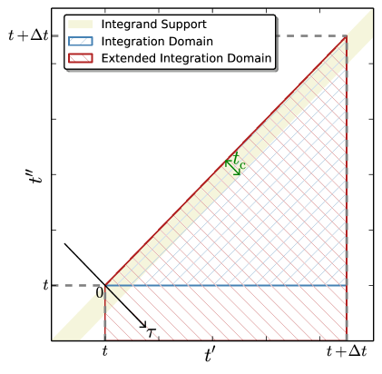
Figure 11: Integration domain of Eq. (A.27) (hatched blue surface). In the limit where $t_{\mathrm{c}}\ll\Delta t$, the extended integration domain (hatched red surface) almost coincides with the initial one when restricted to the region where the integrand is not vanishingly small (pale green surface).

The integration domain appearing in this expression is displayed in Fig. 11 as the hatched blue surface. When parametrised in terms of the variables $t^{\prime}$ and $\tau=t^{\prime}-t^{\prime\prime}$, it is given by

$$\int_{t}^{t+\Delta t}\mathrm{d}t^{\prime}\int_{t}^{t^{\prime}}\mathrm{d}t^{\prime\prime}=\int_{0}^{\Delta t}\mathrm{d}\tau\int_{t+\tau}^{t+\Delta t}\mathrm{d}t^{\prime}\,.$$ (A.28)

Indeed, from Fig. 11, one can see that $\tau$ is comprised between $0$ and $\Delta t$ in the integration domain. Once $\tau$ is fixed, one of the blue lines is described, and it is then clear that $t^{\prime}$ varies between $t+\tau$ and $t+\Delta t$. Because of the terms $C_{R}(\tau)$ and $C_{R}(-\tau)$ in Eq. (A.27), the integrand vanishes when $\left|\tau\right|\gg t_{\mathrm{c}}$, hence its support is given by the pale green stripe in Fig. 11. Let us now consider the extended integration domain

$$\int_{0}^{\infty}\mathrm{d}\tau\int_{t}^{t+\Delta t}\mathrm{d}t^{\prime}\,,$$ (A.29)

where the upper bound on $\tau$ has been extended to infinity and the lower bound on $t^{\prime}$ to $t$. It is displayed as the hatched red surface in Fig. 11. One can see that compared to the initial integration domain, two regions are added. The first one lies outside the integrand support and therefore negligibly contributes to the overall result. The second one is the small triangle that lies inside the integrand support. In the limit where $t_{\mathrm{c}}\ll\Delta t$, it corresponds to a small area compared to the integrand support comprised in the initial integration domain. As a consequence, its inclusion in the integration domain negligibly changes the result if one follows the evolution of the reduced density matrix for the system on time scales $\Delta t$ much larger than the typical correlation time of the environment,

$$t_{\mathrm{c}}\ll\Delta t\,.$$ (A.30)

Under this fifth and last assumption, one then has

$$\tilde{\rho}_{\mathrm{S}}\left(t+\Delta t\right)-\tilde{\rho}_{\mathrm{S}}\left(t\right) \simeq-g^{2}\int_{0}^{\infty}\mathrm{d}\tau\int_{t}^{t+\Delta t}\mathrm{d}t^{\prime}\biggl{\{}\biggl{[}\tilde{A}\left(t^{\prime}\right)\tilde{A}\left(t^{\prime}-\tau\right)\tilde{\rho}_{\mathrm{S}}\left(t^{\prime}-\tau\right)$$ (A.31)

$$-\tilde{A}\left(t^{\prime}-\tau\right)\tilde{\rho}_{\mathrm{S}}\left(t^{\prime}-\tau\right)\tilde{A}\left(t^{\prime}\right)\biggr{]}C_{R}\left(\tau\right)-\biggl{[}\tilde{A}\left(t^{\prime}\right)\tilde{\rho}_{\mathrm{S}}\left(t^{\prime}-\tau\right)\tilde{A}\left(t^{\prime}-\tau\right)$$

$$-\tilde{\rho}_{\mathrm{S}}\left(t^{\prime}-\tau\right)\tilde{A}\left(t^{\prime}-\tau\right)\tilde{A}\left(t^{\prime}\right)\biggr{]}C_{R}\left(-\tau\right)\biggr{\}}\,.$$

The time derivative of $\tilde{\rho}_{\mathrm{S}}$ can then be obtained by dividing the left-hand side and the right-hand side by $\Delta t$. If $\Delta t$ is much smaller than the typical time scale by which $A$ varies, $\tilde{A}(t^{\prime})\simeq\tilde{A}(t)$ and $\tilde{A}(t^{\prime}-\tau)\simeq\tilde{A}(t-\tau)$, the difference only giving rise to $\Delta t$ suppressed quantities. Note that because of that, the condition (A.30) actually means that the interaction operator $A$ should vary on time scales much larger than the autocorrelation time of $R$ in the environment. Moreover, the variation of $\tilde{\rho}_{\mathrm{S}}$ between times $t$ and $t+\Delta t$ in the above integrals is of order $g^{2}$. Since the whole expression is already proportional to $g^{2}$, in the integrals, one can simply write $\tilde{\rho}_{\mathrm{S}}(t)$. As a consequence, the integral over $t^{\prime}$ becomes trivial and $\Delta t$ can be factorised out of the right-hand side, so that

$$\frac{\Delta\tilde{\rho}_{\mathrm{S}}}{\Delta t}= -g^{2}\int_{0}^{\infty}\mathrm{d}\tau\biggl{\{}\left[\tilde{A}\left(t\right)\tilde{A}\left(t-\tau\right)\tilde{\rho}_{\mathrm{S}}\left(t\right)-\tilde{A}\left(t-\tau\right)\tilde{\rho}_{\mathrm{S}}\left(t\right)\tilde{A}\left(t\right)\right]C_{R}(\tau)$$ (A.32)

$$-\left[\tilde{A}\left(t\right)\tilde{\rho}_{\mathrm{S}}\left(t\right)\tilde{A}\left(t-\tau\right)-\tilde{\rho}_{\mathrm{S}}\left(t\right)\tilde{A}\left(t-\tau\right)\tilde{A}\left(t\right)\right]C_{R}(-\tau)\biggr{\}}.$$

This is a Markovian master equation, since the right hand side only depends on $\tilde{\rho}_{\mathrm{S}}$ at time $t$. Defining

$$L_{1}\left(t\right) \equiv g^{2}\int_{0}^{+\infty}\mathrm{d}\tau C_{R}\left(\tau\right)\tilde{A}\left(t-\tau\right),$$ (A.33)

$$L_{2}\left(t\right) \equiv g^{2}\int_{0}^{+\infty}\mathrm{d}\tau C_{R}\left(-\tau\right)\tilde{A}\left(t-\tau\right)=g^{2}\int_{0}^{+\infty}\mathrm{d}\tau C_{R}^{*}\left(\tau\right)\tilde{A}\left(t-\tau\right)=L_{1}^{\dagger}\left(t\right),$$

where the last equality is valid if $\tilde{A}$ is hermitian, it can be written in the more compact form

$$\frac{\Delta\tilde{\rho}_{\mathrm{S}}}{\Delta t}=-\tilde{A}\left(t\right)L_{1}\left(t\right)\tilde{\rho}_{\mathrm{S}}\left(t\right)+L_{1}\left(t\right)\tilde{\rho}_{\mathrm{S}}\left(t\right)\tilde{A}\left(t\right)+\tilde{A}\left(t\right)\tilde{\rho}_{\mathrm{S}}\left(t\right)L_{2}\left(t\right)-\tilde{\rho}_{\mathrm{S}}\left(t\right)L_{2}\left(t\right)\tilde{A}\left(t\right)\,.$$

The operators $L_{1}$ and $L_{2}$ can be further simplified under the condition $t_{\mathrm{c}}\ll\Delta t$. Indeed, because of the profile $C_{R}(\tau)=C_{R}(0)e^{-|\tau|/t_{\mathrm{c}}}$ established above, the integrals $L_{1}$ and $L_{2}$ are dominated by their contribution on the interval $\tau\in[0,\mathrm{a}\ \mathrm{few}\ t_{\mathrm{c}}]$. In the limit where $t_{\mathrm{c}}\ll\Delta t$, the function $\tilde{A}(t-\tau)$ (which, as already said, varies with a typical time scale much larger than $\Delta t$) does not evolve much in this interval and one then has

$$L_{1}\left(t\right)=g^{2}\int_{0}^{+\infty}\mathrm{d}\tau C_{R}\left(\tau\right)\tilde{A}\left(t-\tau\right)\simeq g^{2}\int_{0}^{+\infty}\mathrm{d}\tau C_{R}\left(0\right)e^{-\tau/t_{\mathrm{c}}}\tilde{A}\left(t\right)=g^{2}C_{R}\left(0\right)t_{\mathrm{c}}\tilde{A}\left(t\right)\,,$$ (A.34)

and the same expression for $L_{2}$. As a consequence, Eq. (A) reads

$$\frac{\mathrm{d}\tilde{\rho}_{\mathrm{S}}}{\mathrm{d}t}=-g^{2}C_{R}\left(0\right)t_{\mathrm{c}}\left[\tilde{A},\left[\tilde{A},\tilde{\rho}_{\mathrm{S}}\right]\right]\,.$$ (A.35)

Going back to the standard picture, one finally obtains

$$\frac{\mathrm{d}\rho_{\mathrm{S}}}{\mathrm{d}t}=i\left[\rho_{\mathrm{S}},H_{\mathrm{S}}\right]-g^{2}C_{R}\left(0\right)t_{\mathrm{c}}\left[A,\left[A,\rho_{\mathrm{S}}\right]\right]\,.$$ (A.36)

This is the standard form of the Lindblad equation.

It can be generalised to cases where the interaction term is not simply given by Eq. (A.13), namely by the product of an operator acting in $\mathcal{E}_{\mathrm{S}}$ and an operator acting in $\mathcal{E}_{\mathrm{E}}$. Indeed, if one considers a generic interaction Hamiltonian

$$H_{\mathrm{int}}=\sum_{i}A_{i}\left(t\right)\otimes R_{i}\left(t\right),$$ (A.37)

one can define correlators in the environment as

$$C_{R,ij}\left(t,t^{\prime}\right)\equiv\mathrm{Tr}_{\mathrm{E}}\left[\tilde{\rho}_{\mathrm{E}}\tilde{R}_{i}\left(t\right)\tilde{R}_{j}\left(t^{\prime}\right)\right],$$ (A.38)

and all the previous steps can be repeated, leading to

$$\frac{\mathrm{d}\rho_{\mathrm{S}}}{\mathrm{d}t}=i\left[\rho_{\mathrm{S}},H_{\mathrm{S}}\right]-g^{2}\sum_{i,j}t_{\mathrm{c},ij}C_{R,ij}(0)\left[A_{i},\left[A_{j},\rho_{\mathrm{S}}\right]\right]\,.$$ (A.39)

Here we have assumed that the assumptions discussed before still hold and that $C_{R,ij}=C_{R,ji}$. The characteristic times of the correlation functions $C_{R,ij}$ are denoted $t_{\mathrm{c},ij}$ and must all be much smaller than the typical time scale over which the system varies. If $i$ and $j$ are replaced by continuous indices $\bm{x}$ and $\bm{y}$, the interaction Hamiltonian (A.37) is of the form (2.13), and Eq. (A.39) gives rise to the Lindblad equation (2.16). In this expression $C_{R}(\bm{x},\bm{y})$ denotes $C_{R,ij}(0)$, any potential dependence of $t_{\mathrm{c}}$ on $\bm{x}$ and $\bm{y}$ is absorbed in the function $C_{R}(\bm{x},\bm{y})$, and

$$\gamma=2g^{2}t_{\mathrm{c}}\,.$$ (A.40)

In conclusion, let us summarise the conditions under which the Lindblad equation has been obtained. This equation describes the evolution of the reduced density operator of the system, perturbatively coupled to the environment through an operator $A\otimes R$ where $A$ acts on the system and $R$ on the environment, on time scales much larger than the correlation time of $R$. It is valid only when, in the interaction picture, $\tilde{A}$ varies with time scales much larger than this correlation time. The environment is assumed to be in a stationary state, which technically means that $\langle R\left(t\right)R(t^{\prime})\rangle$ must depend on $t-t^{\prime}$ only, and sufficiently large not to be affected by its interaction with the system. Finally, the above equation is valid if the interaction Hamiltonian has vanishing mean value in the environment, $\langle R\rangle=0$, but this can always be achieved by properly redefining the free and interaction Hamiltonians.

Appendix B Concrete example: a massive scalar field as the environment

In this section, we present a concrete example where the Lindblad formalism can be applied. We consider the case where two scalar fields $\phi$ and $\psi$ are present during inflation, $\phi$ being very light and $\psi$ very heavy. The Fourier modes of $\phi$ play the role of the system, coupled to an environment made of the degrees of freedom contained in $\psi$. This allows us to show how the assumptions used in Appendix A in order to derive Eq. (2.16) can be realised in practice, how the parameters $\gamma$ and $C_{R}(\bm{x},\bm{y})$ that appear in that equation can be related to microphysical quantities, and how the Lindblad operator $A$ can be concretely identified.

Let us consider the following action

$$S=-\int\mathrm{d}^{4}x\mathchoice{{\hbox{$\displaystyle\sqrt{-g\,}$}\lower 0.4pt\hbox{\vrule height=4.30554pt,depth=-3.44446pt}}}{{\hbox{$\textstyle\sqrt{-g\,}$}\lower 0.4pt\hbox{\vrule height=4.30554pt,depth=-3.44446pt}}}{{\hbox{$\scriptstyle\sqrt{-g\,}$}\lower 0.4pt\hbox{\vrule height=3.01389pt,depth=-2.41113pt}}}{{\hbox{$\scriptscriptstyle\sqrt{-g\,}$}\lower 0.4pt\hbox{\vrule height=2.15277pt,depth=-1.72223pt}}}\left[\frac{1}{2}g^{\mu\nu}\partial_{\mu}\phi\partial_{\nu}\phi+V\left(\phi\right)+\frac{1}{2}g^{\mu\nu}\partial_{\mu}\psi\partial_{\nu}\psi+\frac{M^{2}}{2}\psi^{2}+\lambda\mu^{4-n-m}\phi^{n}\psi^{m}\right]\,,$$ (B.1)

where $V(\phi)$ is the potential of the field $\phi$ that we leave unspecified for the moment, $M$ is the mass of the field $\psi$ that we assume to be much larger than the Hubble scale, $M\gg H$, $\lambda$ is a (supposedly small) dimensionless coupling constant and $\mu$ is a mass scale parameter that appears in the power-law coupling between $\phi$ and $\psi$. For now we assume both $\phi$ and $\psi$ to be test fields (i.e. they do not contribute much to the energy budget of the Universe) in an inflating background, but below we comment on how the result can be generalised to the case where $\phi$ is the inflaton field and the system corresponds to the observed cosmological perturbations.

A first important remark is that the action should be written in such a way that the quantum mean value of the interacting term vanishes in the stationary configuration of the environment, as required by Eq. (A.20). Following the procedure described in Appendix A, this can be easily done by adding and subtracting $\lambda\mu^{4-n-m}\left\langle\psi^{m}\right\rangle_{\mathrm{st}}\phi^{n}$,

$$S =-\int\mathrm{d}^{4}x\mathchoice{{\hbox{$\displaystyle\sqrt{-g\,}$}\lower 0.4pt\hbox{\vrule height=4.30554pt,depth=-3.44446pt}}}{{\hbox{$\textstyle\sqrt{-g\,}$}\lower 0.4pt\hbox{\vrule height=4.30554pt,depth=-3.44446pt}}}{{\hbox{$\scriptstyle\sqrt{-g\,}$}\lower 0.4pt\hbox{\vrule height=3.01389pt,depth=-2.41113pt}}}{{\hbox{$\scriptscriptstyle\sqrt{-g\,}$}\lower 0.4pt\hbox{\vrule height=2.15277pt,depth=-1.72223pt}}}\left[\frac{1}{2}g^{\mu\nu}\partial_{\mu}\phi\partial_{\nu}\phi+V\left(\phi\right)+\lambda\mu^{4-n-m}\left\langle\psi^{m}\right\rangle_{\mathrm{st}}\phi^{n}\right.$$ (B.2)

$$\left.+\frac{1}{2}g^{\mu\nu}\partial_{\mu}\psi\partial_{\nu}\psi+\frac{M^{2}}{2}\psi^{2}+\lambda\mu^{4-n-m}\phi^{n}\left(\psi^{m}-\left\langle\psi^{m}\right\rangle_{\mathrm{st}}\right)\right]\,,$$

where $\left\langle\psi^{m}\right\rangle_{\mathrm{st}}$ denotes the stationary quantum mean value of $\psi^{m}$. This simply modifies the effective potential of the field $\phi$ according to

$$V_{\mathrm{eff}}(\phi)=V(\phi)+\lambda\mu^{4-n-m}\left\langle\psi^{m}\right\rangle_{\mathrm{st}}\phi^{n}\,.$$ (B.3)

On the other hand, it is now clear that the mean value of the interacting term taken in the environment sector, $\psi^{m}-\left\langle\psi^{m}\right\rangle_{\mathrm{st}}$, vanishes. The action (B.2) can be decomposed as $S=S_{\phi}+S_{\psi}+S_{\phi\psi}$, and $S_{\phi\psi}$ gives rise to the interaction Hamiltonian

$$H_{\mathrm{int}}=\lambda\mu^{4-n-m}a^{4}\int\mathrm{d}^{3}{\bm{x}}\,\phi^{n}\left(\psi^{m}-\left\langle\psi^{m}\right\rangle_{\mathrm{st}}\right)\,.$$ (B.4)

Assuming that $V_{\mathrm{eff}}(\phi)=m^{2}\phi^{2}/2$, in Fourier space, one has

$$S_{\phi} =\frac{1}{2}\int\mathrm{d}\eta\int_{\mathbb{R}^{3}}\mathrm{d}^{3}{\bm{k}}\left[v_{\bm{k}}^{\prime}v_{\bm{k}}^{*}{}^{\prime}-\left(k^{2}-\frac{a^{\prime\prime}}{a}+m^{2}a^{2}\right)v_{\bm{k}}v_{\bm{k}}^{*}\right],$$ (B.5)

where we have defined $v(\eta,{\bm{x}})\equiv a(\eta)\phi(\eta,{\bm{x}})$. If one lets $m=0$ in Eq. (B.5), then one recovers the action for curvature perturbations if one ignores metric perturbations (and it is even exactly the same for the particular case of power-law inflation). This suggests that, by identifying the variable $v(\eta,{\bm{x}})$ with the Mukhanov-Sasaki variable (which is the reason why we have used the same notation) in the uniform-curvature gauge, we can extend the present analysis to the case where $\phi$ is the inflaton field and the system corresponds to the curvature perturbations.

In terms of the Mukhanov-Sasaki variable, the interaction Hamiltonian is given by

$$H_{\mathrm{int}}=\lambda\mu^{4-n-m}a^{4-n}\int\mathrm{d}^{3}{\bm{x}}\,v^{n}\left(\eta,{\bm{x}}\right)\left[\psi^{m}\left(\eta,{\bm{x}}\right)-\left\langle\psi^{m}\right\rangle_{\mathrm{st}}\right]\,.$$ (B.6)

This is of the form (2.13) provided $A=v^{n}$, $R=\psi^{m}-\left\langle\psi^{m}\right\rangle_{\mathrm{st}}$, and the effective coupling constant reads $g=\lambda\mu^{4-n-m}a^{4-n}$ which is, therefore, a time-dependent quantity. In Appendix A, we have showed that $\gamma=2g^{2}\tau_{\mathrm{{c}}}$, see Eq. (A.40). In this expression, $\tau_{\mathrm{{c}}}$ is the correlation time of $R$. Given that, in the main text, the Lindblad equation is written in terms of conformal time, $\tau_{\mathrm{{c}}}$ in this context must be interpreted as a conformal correlation time and expressed as $t_{\mathrm{c}}/a$, $t_{\mathrm{c}}$ being the cosmic correlation time. This implies that the ansatz (2.18) is satisfied, $\gamma=\gamma_{*}(a/a_{*})^{p}$, if we make the identification

$$\gamma_{*}=2t_{\mathrm{c}}\lambda^{2}\mu^{8-2n-2m}a_{*}^{7-2n}$$ (B.7)

and $p=7-2n$. For a linear interaction, this leads to $p=5$ and for a quadratic interaction, one has $p=3$.

The explicit form of $R$ also allows us to calculate the correlation function $C_{R}$. Massive fields in de-Sitter space-times have long been studied [92, 61, 62, 63]. In the small-separation limit, $\epsilon^{2}\equiv[(t_{1}-t_{2})^{2}-a^{2}({\bm{x}}_{1}-{\bm{x}}_{2})^{2}]/4\ll\mathrm{min}(1/H^{2},1/M^{2})$, point-splitting renormalisation yields the two-point correlation function given by Eq. (3.14) in LABEL:Bunch:1978yq. In the regime where $M\gg H$, expanding this formula in powers of $H/M$ leads to

$$\left\langle\psi\left(t_{1},{\bm{x}}_{1}\right)\psi\left(t_{2},{\bm{x}}_{2}\right)\right\rangle_{\mathrm{ren}}\simeq\frac{37}{504\pi^{2}}\frac{H^{6}}{M^{4}}\left(1-\frac{M^{2}\Sigma\epsilon^{2}}{2}\right)$$ (B.8)

at leading order in $H/M$, where $\Sigma=\pm 1$ depends on whether the separation between the two points $(t_{1},\bm{x}_{1})$ and $(t_{2},\bm{x}_{2})$ is timelike or spacelike. Assuming that $\psi$ has Gaussian statistics (which is correct at leading order in perturbation theory), Wick theorem leads to

$$\left\langle\psi^{m}\left(t_{1},{\bm{x}}_{1}\right)\psi^{m}\left(t_{2},{\bm{x}}_{2}\right)\right\rangle_{\mathrm{ren}}\simeq$$ (B.9)

$$\sum_{0\leq p\leq\left\lfloor\frac{m}{2}\right\rfloor}a_{p,m}\left\langle\psi\left(t_{1},{\bm{x}}_{1}\right)\psi\left(t_{1},{\bm{x}}_{1}\right)\right\rangle_{\mathrm{ren}}^{p}\left\langle\psi\left(t_{2},{\bm{x}}_{2}\right)\psi\left(t_{2},{\bm{x}}_{2}\right)\right\rangle_{\mathrm{ren}}^{p}\left\langle\psi\left(t_{1},{\bm{x}}_{1}\right)\psi\left(t_{2},{\bm{x}}_{2}\right)\right\rangle_{\mathrm{ren}}^{m-2p}\,.$$

In this expression, $\lfloor m/2\rfloor$ denotes the integer part of $m/2$, i.e. it is $m/2$ is $m$ is even and $(m-1)/2$ if $m$ is odd, and $a_{p,m}$ are combinatory coefficients that can be calculated as follows. In the product of pairs written in the sum of Eq. (LABEL:eq:massivefield:corr:higher:order:start), $2p$ is the number of $\psi(t_{1},\bm{x_{1}})$ occurrences that go into auto-correlators and $m-2p$ is the number of $\psi(t_{1},\bm{x_{1}})$ occurrences that go into cross-correlators. The number of ways to split the $m$ occurrences of $\psi(t_{1},\bm{x_{1}})$ between these two types of correlators is given by ${{m}\choose{2p}}=m!/[(2p)!(m-2p)!]$, i.e. by the number of ways one can draw $2p$ elements out of $m$ elements (or equivalently $m-2p$ elements out of $m$ elements). The same applies for dispatching the occurrences of $\psi(t_{2},\bm{x_{2}})$. Then, once the $2p$ occurrences of $\psi(t_{1},\bm{x_{1}})$ that appear in auto-correlators are chosen, one has to arrange them into pairs, and the number of such arrangements is given by $(2p-1)!!=(2p)!/(2^{p}p!)$. The same applies for arranging into pairs the $2p$ occurrences of $\psi(t_{2},\bm{x_{2}})$ that go into auto-correlators. Finally, the number of cross-correlators one can build from the $m-2p$ occurrences of $\psi(t_{1},\bm{x_{1}})$ and $\psi(t_{2},\bm{x_{2}})$ is given by $(m-2p)!$. Putting everything together, one obtains

$$a_{p,m}=\left[{{m}\choose{2p}}(2p-1)!!\right]^{2}(m-2p)!=\frac{\left(m!\right)^{2}}{2^{2p}\left(p!\right)^{2}\left(m-2p\right)!}\,.$$ (B.10)

Combining Eqs. (B.8) and (LABEL:eq:massivefield:corr:higher:order:start), one also has

$$\left\langle\psi^{m}\left(t_{1},{\bm{x}}_{1}\right)\psi^{m}\left(t_{2},{\bm{x}}_{2}\right)\right\rangle_{\mathrm{ren}} \simeq\left(\frac{37}{504\pi^{2}}\frac{H^{6}}{M^{4}}\right)^{m}\sum_{0\leq p\leq\left\lfloor\frac{m}{2}\right\rfloor}a_{p,m}\left(1-\frac{M^{2}\Sigma\epsilon^{2}}{2}\right)^{m-2p}$$ (B.11)

$$\simeq\left(\frac{37}{504\pi^{2}}\frac{H^{6}}{M^{4}}\right)^{m}\sum_{0\leq p\leq\left\lfloor\frac{m}{2}\right\rfloor}a_{p,m}\left[1-\left(m-2p\right)\frac{M^{2}\Sigma\epsilon^{2}}{2}\right]\,,$$

where in the second line we have expanded in the small $\epsilon$ limit. This expression requires to calculate two sums involving the combinatory coefficients $a_{p,m}$. The first one is straightforward,

$$\sum_{0\leq p\leq\left\lfloor\frac{m}{2}\right\rfloor}a_{p,m}=\left(2m-1\right)!!\,,$$ (B.12)

since it corresponds by definition to the number of arrangements of the $2m$ occurrences of $\psi$ into pairs. Making use of Eq. (B.10), the second sum is given by

$$\sum_{0\leq p\leq\left\lfloor\frac{m}{2}\right\rfloor}\left(m-2p\right)a_{p,m} =\sum_{0\leq p\leq\left\lfloor\frac{m}{2}\right\rfloor}\left(m-2p\right)\frac{\left(m!\right)^{2}}{2^{2p}\left(p!\right)^{2}\left(m-2p\right)!}$$ (B.13)

$$=\sum_{0\leq p\leq\left\lfloor\frac{m-1}{2}\right\rfloor}\left(m-2p\right)\frac{\left(m!\right)^{2}}{2^{2p}\left(p!\right)^{2}\left(m-2p\right)!}$$

$$=m^{2}\sum_{0\leq p\leq\left\lfloor\frac{m-1}{2}\right\rfloor}\frac{\left[\left(m-1\right)!\right]^{2}}{2^{2p}\left(p!\right)^{2}\left(m-1-2p\right)!}$$

$$=m^{2}\sum_{0\leq p\leq\left\lfloor\frac{m-1}{2}\right\rfloor}a_{p,m-1}$$

$$=m^{2}\left(2m-3\right)!!\,.$$

In the second line of this derivation, we have used the fact that if $m$ is even, the last term of the sum corresponds to $p=m/2$, which vanishes because of the coefficient $m-2p$, so one can stop the sum at $p=\lfloor(m-1)/2\rfloor$, and in the last line, we have used Eq. (B.12). Then, plugging Eqs. (B.12) and (B.13) into Eq. (B.11), one obtains

$$\left\langle\psi^{m}\left(t_{1},{\bm{x}}_{1}\right)\psi^{m}\left(t_{2},{\bm{x}}_{2}\right)\right\rangle_{\mathrm{ren}}\simeq\left(2m-1\right)!!\left(\frac{37}{504\pi^{2}}\frac{H^{6}}{M^{4}}\right)^{m}\left(1-\frac{m^{2}}{2m-1}\frac{M^{2}\Sigma\epsilon^{2}}{2}\right)\,.$$ (B.14)

Wick theorem with Eq. (B.8) also gives rise to

$$\left\langle\psi^{m}\right\rangle_{\mathrm{st}} =\sigma(m)\left(m-1\right)!!\left(\frac{37}{504\pi^{2}}\frac{H^{6}}{M^{4}}\right)^{\frac{m}{2}}\,,$$ (B.15)

where $\sigma(m)=1$ if $m$ is even and $0$ is $m$ is odd. Notice that this equation is consistent with Eq. (B.14). Recalling that $R=\psi^{m}-\left\langle\psi^{m}\right\rangle_{\mathrm{st}}$, Eq. (A.38) gives rise to

$$C_{R}\left(t_{1},{\bm{x}}_{1};t_{2},{\bm{x}}_{2}\right)=\left\langle\psi^{m}\left(t_{1},{\bm{x}}_{1}\right)\psi^{m}\left(t_{2},{\bm{x}}_{2}\right)\right\rangle_{\mathrm{ren}}-\left\langle\psi^{m}\right\rangle_{\mathrm{st}}^{2}\,,$$ (B.16)

where we have used that $\langle\psi^{m}\rangle_{\mathrm{st}}$ is independent of time (which is in fact required by stationarity) and space. Inserting Eqs. (B.14) and (B.15) into this expression, one obtains

$$C_{R}\left(t_{1},{\bm{x}}_{1};t_{2},{\bm{x}}_{2}\right)= \left\{\left(2m-1\right)!!-\sigma\left(m\right)\left[\left(m-1\right)!!\right]^{2}\right\}\left(\frac{37}{504\pi^{2}}\frac{H^{6}}{M^{4}}\right)^{m}\times$$ (B.17)

$$\left\{1-\frac{m^{2}\left(2m-3\right)!!}{\left(2m-1\right)!!-\sigma\left(m\right)\left[\left(m-1\right)!!\right]^{2}}\frac{M^{2}\Sigma\epsilon^{2}}{2}\right\}\,.$$

From this formula, the overall amplitude $\bar{C}_{R}$, the correlation cosmic time $t_{\mathrm{c}}$ and the correlation length $\ell_{\mathrm{E}}$ of the two-point function of $R$ in the environment can be read off and are given by

$$\bar{C}_{R} =\left\{\left(2m-1\right)!!-\sigma\left(m\right)\left[\left(m-1\right)!!\right]^{2}\right\}\left(\frac{37}{504\pi^{2}}\frac{H^{6}}{M^{4}}\right)^{m}\,,$$ (B.18)

$$t_{\mathrm{c}} =\ell_{\mathrm{E}}=2\mathchoice{{\hbox{$\displaystyle\sqrt{2\,}$}\lower 0.4pt\hbox{\vrule height=6.44444pt,depth=-5.15558pt}}}{{\hbox{$\textstyle\sqrt{2\,}$}\lower 0.4pt\hbox{\vrule height=6.44444pt,depth=-5.15558pt}}}{{\hbox{$\scriptstyle\sqrt{2\,}$}\lower 0.4pt\hbox{\vrule height=4.51111pt,depth=-3.6089pt}}}{{\hbox{$\scriptscriptstyle\sqrt{2\,}$}\lower 0.4pt\hbox{\vrule height=3.22221pt,depth=-2.57779pt}}}\mathchoice{{\hbox{$\displaystyle\sqrt{\frac{\left(2m-1\right)!!-\sigma\left(m\right)\left[\left(m-1\right)!!\right]^{2}}{m^{2}\left(2m-3\right)!!}\,}$}\lower 0.4pt\hbox{\vrule height=16.80444pt,depth=-13.44362pt}}}{{\hbox{$\textstyle\sqrt{\frac{\left(2m-1\right)!!-\sigma\left(m\right)\left[\left(m-1\right)!!\right]^{2}}{m^{2}\left(2m-3\right)!!}\,}$}\lower 0.4pt\hbox{\vrule height=11.78888pt,depth=-9.43115pt}}}{{\hbox{$\scriptstyle\sqrt{\frac{\left(2m-1\right)!!-\sigma\left(m\right)\left[\left(m-1\right)!!\right]^{2}}{m^{2}\left(2m-3\right)!!}\,}$}\lower 0.4pt\hbox{\vrule height=8.78888pt,depth=-7.03114pt}}}{{\hbox{$\scriptscriptstyle\sqrt{\frac{\left(2m-1\right)!!-\sigma\left(m\right)\left[\left(m-1\right)!!\right]^{2}}{m^{2}\left(2m-3\right)!!}\,}$}\lower 0.4pt\hbox{\vrule height=8.78888pt,depth=-7.03114pt}}}\frac{1}{M}\,.$$

In particular, with Eq. (B.7) this gives rise to

$$\gamma_{*}=4\mathchoice{{\hbox{$\displaystyle\sqrt{2\,}$}\lower 0.4pt\hbox{\vrule height=6.44444pt,depth=-5.15558pt}}}{{\hbox{$\textstyle\sqrt{2\,}$}\lower 0.4pt\hbox{\vrule height=6.44444pt,depth=-5.15558pt}}}{{\hbox{$\scriptstyle\sqrt{2\,}$}\lower 0.4pt\hbox{\vrule height=4.51111pt,depth=-3.6089pt}}}{{\hbox{$\scriptscriptstyle\sqrt{2\,}$}\lower 0.4pt\hbox{\vrule height=3.22221pt,depth=-2.57779pt}}}\mathchoice{{\hbox{$\displaystyle\sqrt{\frac{\left(2m-1\right)!!-\sigma\left(m\right)\left[\left(m-1\right)!!\right]^{2}}{m^{2}\left(2m-3\right)!!}\,}$}\lower 0.4pt\hbox{\vrule height=16.80444pt,depth=-13.44362pt}}}{{\hbox{$\textstyle\sqrt{\frac{\left(2m-1\right)!!-\sigma\left(m\right)\left[\left(m-1\right)!!\right]^{2}}{m^{2}\left(2m-3\right)!!}\,}$}\lower 0.4pt\hbox{\vrule height=11.78888pt,depth=-9.43115pt}}}{{\hbox{$\scriptstyle\sqrt{\frac{\left(2m-1\right)!!-\sigma\left(m\right)\left[\left(m-1\right)!!\right]^{2}}{m^{2}\left(2m-3\right)!!}\,}$}\lower 0.4pt\hbox{\vrule height=8.78888pt,depth=-7.03114pt}}}{{\hbox{$\scriptscriptstyle\sqrt{\frac{\left(2m-1\right)!!-\sigma\left(m\right)\left[\left(m-1\right)!!\right]^{2}}{m^{2}\left(2m-3\right)!!}\,}$}\lower 0.4pt\hbox{\vrule height=8.78888pt,depth=-7.03114pt}}}\frac{\lambda^{2}}{M}\mu^{8-2n-2m}a_{*}^{7-2n}\,.$$ (B.19)

Let us also note that in Eq. (B.18), $\bar{C}_{R}$ is proportional to $H^{6m}$. In a Universe that is inflating in the slow-roll regime, $H$ is not strictly constant but scales as $a^{-\epsilon_{1}}$, where $\epsilon_{1}$ is the first slow-roll parameter. This slow time variation can be absorbed in $p$ by replacing $p\rightarrow p-6m\epsilon_{1*}$, leading to

$$p=7-2n-6m\epsilon_{1*}\,,$$ (B.20)

and replacing $H$ with $H_{*}$ in Eq. (B.18). Let us note that this assumes that Eq. (B.8) is valid even when $H$ varies with time. In that case however, there is no known analytical solution for the two-point correlation function of the field $\psi$ (however, in the case $H\propto a^{-\epsilon_{1}}$, see LABEL:Janssen:2009pb). Nevertheless, since $M\gg H$, the relaxation time of this correlation function, $1/M$, is much smaller than the typical time scale over which $H$ varies, $1/(H\epsilon_{1})$, and one can assume $\psi$ to adiabatically follow Eq. (B.8).

In Appendix A, it was made clear that the Lindblad equation relies on the validity of a number of assumptions. Let us now derive the conditions under which those assumptions are verified in the simple model considered here.

First, one needs to check that $\psi$ is a test field (strictly speaking this is not a required condition for the derivation of the Lindblad equation but is necessary for the consistency of the model presented here). In order for $\psi$ to play a negligible role in the energy budget of the Universe, $M^{2}\left\langle\psi^{2}\right\rangle_{\mathrm{st}}$ has to be small compared to the total energy density of the Universe $\rho$,

$$M^{2}\left\langle\psi^{2}\right\rangle_{\mathrm{st}}\ll 3M_{\scriptscriptstyle{\mathrm{Pl}}}^{2}H^{2}\,,$$ (B.21)

where the Friedmann equation $\rho=3M_{\scriptscriptstyle{\mathrm{Pl}}}^{2}H^{2}$ has been used. Making use of Eq. (B.15) with $m=2$, one has

$$\frac{M^{2}\left\langle\psi^{2}\right\rangle_{\mathrm{st}}}{3M_{\scriptscriptstyle{\mathrm{Pl}}}^{2}H^{2}}=\frac{37}{1512\pi^{2}}\frac{H^{4}}{M^{2}M_{\scriptscriptstyle{\mathrm{Pl}}}^{2}}\,.$$ (B.22)

Since $M\gg H$, and since $H/M_{\scriptscriptstyle{\mathrm{Pl}}}\lesssim 10^{-4}$ due to the current observational bound [70] on the tensor-to-scalar ratio, this number is necessarily very small and the condition is satisfied.

Second, if $\phi$ is taken to be a test field, a similar condition must be satisfied, $V_{\mathrm{eff}}(\phi)\ll 3M_{\scriptscriptstyle{\mathrm{Pl}}}^{2}H^{2}$, where $V_{\mathrm{eff}}(\phi)$ is given in Eq. (B.3). Assuming that the initial potential $V(\phi)$ is such that $\phi$ is indeed a test field, $V(\phi)\ll 3M_{\scriptscriptstyle{\mathrm{Pl}}}^{2}H^{2}$, the condition $V_{\mathrm{eff}}(\phi)\ll 3M_{\scriptscriptstyle{\mathrm{Pl}}}^{2}H^{2}$ reduces to

$$\lambda\mu^{4-n-m}\left\langle\psi^{m}\right\rangle_{\mathrm{st}}\phi^{n}\ll 3M_{\scriptscriptstyle{\mathrm{Pl}}}^{2}H^{2}\,.$$ (B.23)

If, on the other hand, $\phi$ is taken to be the inflaton field, one must ensure that the correction to its potential arising in Eq. (B.3) does not spoil its flatness. If Eq. (B.23) is satisfied, this is obviously the case since $3M_{\scriptscriptstyle{\mathrm{Pl}}}^{2}H^{2}\simeq V(\phi)$ in the slow-roll approximation and Eq. (B.23) implies that $V_{\mathrm{eff}}(\phi)\simeq V(\phi)$. The condition (B.23) also guarantees that the effect of the environment on the system can be treated perturbatively. Making use of Eq. (B.15), it can also be expressed as

$$\frac{\lambda\mu^{4-n-m}\left\langle\psi^{m}\right\rangle_{\mathrm{st}}\phi^{n}}{3M_{\scriptscriptstyle{\mathrm{Pl}}}^{2}H^{2}}=\sigma(m)\frac{\left(m-1\right)!!}{3}\left(\frac{37}{504\pi^{2}}\right)^{\frac{m}{2}}\lambda\frac{\mu^{4-n-m}\phi^{n}H^{3m-2}}{M_{\scriptscriptstyle{\mathrm{Pl}}}^{2}M^{2m}}\ll 1\,.$$ (B.24)

This means that, in practice, the coupling constant must be sufficiently small, but the constraint depends on the value of $\phi$ which can only be specified by choosing an explicit model.

Third, one must check that the interaction term does not affect much the behaviour of the environment. This means that

$$\lambda\mu^{4-n-m}\phi^{n}\psi^{m}\ll M^{2}\psi^{2}\,.$$ (B.25)

Notice that because of Eq. (B.21), this condition ensures that Eq. (B.23) is satisfied too. Making use of Eq. (B.15), one has

$$\frac{\lambda\mu^{4-n-m}\phi^{n}\left\langle\psi^{m}\right\rangle_{\mathrm{st}}}{M^{2}\left\langle\psi^{2}\right\rangle_{\mathrm{st}}}=\left(m-1\right)!!\left(\frac{37}{504\pi^{2}}\right)^{\frac{m}{2}-1}\lambda\frac{\mu^{4-n-m}\phi^{n}}{H^{6-3m}M^{2m-2}}\,.$$ (B.26)

Again, this condition is verified if the coupling constant $\lambda$ is sufficiently small, but the precise upper bound on $\lambda$ depends on the value of $\phi$ which has to be specified by choosing a model.

Fourth, one needs to make sure that, when the environment is in its stationary state, $R=\psi^{m}-\left\langle\psi^{m}\right\rangle_{\mathrm{st}}$ has autocorrelation time $t_{\mathrm{c}}$ much smaller than the typical time scale for the evolution of the system in the interaction picture, noted $\tilde{T}_{A}$. Since the system is a light scalar field, it evolves with a time scale that is typically of order $H^{-1}$. In the interaction picture, the terms $\exp(i\int H_{v})$ must be included as well, but the pulsation $\omega^{2}$ given in Eq. (2.3) also gives rise to variations over the Hubble time, such that $\tilde{T}_{A}=H^{-1}$. Given that $t_{\mathrm{c}}\sim 1/M$, see Eq. (B.18), one has

$$\frac{t_{\mathrm{c}}}{\tilde{T}_{A}}\sim\frac{H}{M}\,.$$ (B.27)

Since we assumed $\psi$ to be a heavy field, $M\gg H$, the condition $t_{\mathrm{c}}\ll\tilde{T}_{A}$ is always satisfied.

Appendix C Density matrix for linear interaction

In this appendix, we show how the equation (3.6) for the elements of the density matrix in the basis $|v_{\bm{k}}^{s}\rangle$ and in presence of linear interaction can be solved. Let us consider $\left\langle v^{s,(1)}_{\bm{k}}\right|\hat{\rho}_{\bm{k}}^{s}\left|v^{s,(2)}_{\bm{k}}\right\rangle\equiv f(d,D,\eta)$ as a generic function of

$$d=v^{s,(2)}_{\bm{k}}-v^{s,(1)}_{\bm{k}}\,,\qquad D=\frac{v^{s,(1)}_{\bm{k}}+v^{s,(2)}_{\bm{k}}}{2}$$ (C.1)

and conformal time $\eta$, where we have dropped the dependence on $s$ and $\bm{k}$ of the variables $d$ and $D$ in order not to cluster notations too much (strictly speaking one should write $d^{s}_{\bm{k}}$ and $D^{s}_{\bm{k}}$, but since the Lindblad equation factorises into independent equations in each Fourier subspace, no confusion can arise). Written in terms of $d$ and $D$, Eq. (3.6) takes the form

$$\frac{\partial f\left(d,D,\eta\right)}{\partial\eta}=\left[-i\frac{\partial}{\partial d}\frac{\partial}{\partial D}+i\omega^{2}\left(k\right)dD-\frac{\gamma}{2}\left(2\pi\right)^{3/2}\tilde{C}_{R}(\bm{k})d^{2}\right]f\left(d,D,\eta\right)\,.$$ (C.2)

This is a linear partial differential equation of order $2$ with respect to the three variables $d$, $D$ and $\eta$.

C.1 General solution

This equation can be cast as a family of first-order partial differential equations if we Fourier transform the $D$ coordinate, namely by introducing

$$f\left(d,D,\eta\right)=\frac{1}{\mathchoice{{\hbox{$\displaystyle\sqrt{2\pi\,}$}\lower 0.4pt\hbox{\vrule height=6.44444pt,depth=-5.15558pt}}}{{\hbox{$\textstyle\sqrt{2\pi\,}$}\lower 0.4pt\hbox{\vrule height=6.44444pt,depth=-5.15558pt}}}{{\hbox{$\scriptstyle\sqrt{2\pi\,}$}\lower 0.4pt\hbox{\vrule height=4.51111pt,depth=-3.6089pt}}}{{\hbox{$\scriptscriptstyle\sqrt{2\pi\,}$}\lower 0.4pt\hbox{\vrule height=3.22221pt,depth=-2.57779pt}}}}\int\mathrm{d}re^{irD}\tilde{f}\left(d,r,\eta\right)\,.$$ (C.3)

Plugging this expansion into Eq. (C.2), the Fourier component $\tilde{f}(d,r,\eta)$ can be shown to obey the following equation

$$\frac{\partial\tilde{f}\left(d,r,\eta\right)}{\partial\eta}=\left[r\frac{\partial}{\partial d}-\omega^{2}\left(k\right)d\frac{\partial}{\partial r}-\frac{\gamma}{2}\left(2\pi\right)^{3/2}\tilde{C}_{R}(\bm{k})d^{2}\right]\tilde{f}\left(d,r,\eta\right)\,.$$ (C.4)

This is now a linear first-order partial differential equation and, therefore, it can be solved with the method of characteristics. To this end let us considered a characteristic line $\eta(\tau)$, $r(\tau)$ and $d(\tau)$ in the three dimensional space $(\eta,r,d)$, parametrised by the curvilinear coordinate $\tau$. Along this line, $\tilde{f}$ is a function of $\tau$ only and Eq. (C.4) allows us to write

$$\frac{\mathrm{d}}{\mathrm{d}\tau}\tilde{f}\left[d\left(\tau\right),r\left(\tau\right),\eta\left(\tau\right)\right] =\Bigg{\{}\left[r\left(\tau\right)\eta^{\prime}\left(\tau\right)+d^{\prime}\left(\tau\right)\right]\frac{\partial}{\partial d}+\left[r^{\prime}\left(\tau\right)-\omega^{2}\left(k\right)d\left(\tau\right)\eta^{\prime}\left(\tau\right)\right]\frac{\partial}{\partial r}$$ (C.5)

$$-\frac{\gamma}{2}\left(2\pi\right)^{3/2}\tilde{C}_{R}\left(\bm{k}\right)d^{2}\left(\tau\right)\eta^{\prime}\left(\tau\right)\Bigg{\}}\tilde{f}\left[d\left(\tau\right),r\left(\tau\right),\eta\left(\tau\right)\right]\,,$$

where a prime here denotes derivation with respect to $\tau$. In order to remove the contribution from the partial derivatives along $d$ and $r$ in this equation, let us now choose the characteristic line such that it satisfies

$$\eta^{\prime}\left(\tau\right)=1\,,\qquad d^{\prime}\left(\tau\right)=-r(\tau)\,,\qquad r^{\prime}\left(\tau\right)=\omega^{2}\left(k\right)d(\tau),$$ (C.6)

i.e. in such a way that Eq. (C.5) can be written as an ordinary differential equation of the variable $\tau$ only, namely

$$\frac{\mathrm{d}\tilde{f}}{\mathrm{d}\tau}=-\frac{\gamma}{2}(2\pi)^{3/2}\tilde{C}_{R}(\bm{k})d^{2}\tilde{f}.$$ (C.7)

Let us now specify the initial conditions. Requiring the initial state to be in the Bunch-Davies vacuum, one has

$$\tilde{f}\left(d_{\mathrm{in}},r_{\mathrm{in}},\eta_{\mathrm{in}}\right)\underset{k\eta_{\mathrm{in}}\rightarrow-\infty}{\longrightarrow}\frac{1}{\mathchoice{{\hbox{$\displaystyle\sqrt{2\pi\,}$}\lower 0.4pt\hbox{\vrule height=6.44444pt,depth=-5.15558pt}}}{{\hbox{$\textstyle\sqrt{2\pi\,}$}\lower 0.4pt\hbox{\vrule height=6.44444pt,depth=-5.15558pt}}}{{\hbox{$\scriptstyle\sqrt{2\pi\,}$}\lower 0.4pt\hbox{\vrule height=4.51111pt,depth=-3.6089pt}}}{{\hbox{$\scriptscriptstyle\sqrt{2\pi\,}$}\lower 0.4pt\hbox{\vrule height=3.22221pt,depth=-2.57779pt}}}}e^{-\frac{kd^{2}_{\mathrm{in}}}{4}-\frac{r^{2}_{\mathrm{in}}}{4k}}\,.$$ (C.10)

With this initial condition, the solution of Eq. (C.7) can be found and reads

$$\tilde{f}\left[d\left(\tau\right),r\left(\tau\right),\eta\left(\tau\right)\right]=\frac{e^{-\frac{kd^{2}_{\mathrm{in}}}{4}-\frac{r^{2}_{\mathrm{in}}}{4k}}}{\mathchoice{{\hbox{$\displaystyle\sqrt{2\pi\,}$}\lower 0.4pt\hbox{\vrule height=6.44444pt,depth=-5.15558pt}}}{{\hbox{$\textstyle\sqrt{2\pi\,}$}\lower 0.4pt\hbox{\vrule height=6.44444pt,depth=-5.15558pt}}}{{\hbox{$\scriptstyle\sqrt{2\pi\,}$}\lower 0.4pt\hbox{\vrule height=4.51111pt,depth=-3.6089pt}}}{{\hbox{$\scriptscriptstyle\sqrt{2\pi\,}$}\lower 0.4pt\hbox{\vrule height=3.22221pt,depth=-2.57779pt}}}}\exp\left\{-\frac{(2\pi)^{3/2}}{2}\int_{\tau_{\mathrm{in}}}^{\tau}\mathrm{d}\tau^{\prime}\gamma\left[\eta\left(\tau^{\prime}\right)\right]\,\tilde{C}_{R}\left[\bm{k},\eta\left(\tau^{\prime}\right)\right]\,d^{2}(\tau^{\prime})\right\}\,.$$ (C.11)

One still needs to solve for the functions $\eta\left(\tau\right)$ and $d(\tau)$ since these functions appear in the above expression. This can be done through the integration of Eqs. (C.6), which leads to

$$\eta(\tau) =\tau,$$ (C.12)

$$d\left(\tau\right) =u_{\bm{k}}\left(\tau\right)d_{\mathrm{in}}+w_{\bm{k}}\left(\tau\right)r_{\mathrm{in}}\,,$$ (C.13)

$$r\left(\tau\right) =-u_{\bm{k}}^{\prime}\left(\tau\right)d_{\mathrm{in}}-w_{\bm{k}}^{\prime}\left(\tau\right)r_{\mathrm{in}}\,.$$ (C.14)

Here we have chosen the first integration constant such that $\eta_{\mathrm{in}}=\tau_{\mathrm{in}}$, and since $d(\tau)$ and $r(\tau)$ satisfy two coupled linear first-order differential equations, we have simply written that $d$ is a linear combination of $d_{\mathrm{in}}$ and $r_{\mathrm{in}}$, and calculated $r=-d^{\prime}$ accordingly. The two real functions $u_{\bm{k}}$ and $w_{\bm{k}}$ (where the dependence on $\bm{k}$ has been reestablished) will be calculated below, but for now, plugging Eqs. (C.12) and (C.13) into Eq. (C.11), one obtains

$$\tilde{f}\left(d,r,\eta\right)=$$ (C.15)

$$\qquad\quad\frac{e^{-\frac{kd^{2}_{\mathrm{in}}}{4}-\frac{r^{2}_{\mathrm{in}}}{4k}}}{\mathchoice{{\hbox{$\displaystyle\sqrt{2\pi\,}$}\lower 0.4pt\hbox{\vrule height=6.44444pt,depth=-5.15558pt}}}{{\hbox{$\textstyle\sqrt{2\pi\,}$}\lower 0.4pt\hbox{\vrule height=6.44444pt,depth=-5.15558pt}}}{{\hbox{$\scriptstyle\sqrt{2\pi\,}$}\lower 0.4pt\hbox{\vrule height=4.51111pt,depth=-3.6089pt}}}{{\hbox{$\scriptscriptstyle\sqrt{2\pi\,}$}\lower 0.4pt\hbox{\vrule height=3.22221pt,depth=-2.57779pt}}}}\exp\left\{-\frac{(2\pi)^{3/2}}{2}\int_{\eta_{\mathrm{in}}}^{\eta}\mathrm{d}\eta^{\prime}\gamma\left(\eta^{\prime}\right)\,\tilde{C}_{R}\left(\bm{k},\eta^{\prime}\right)\,\left[u_{\bm{k}}\left(\eta^{\prime}\right)d_{\mathrm{in}}+w_{\bm{k}}\left(\eta^{\prime}\right)r_{\mathrm{in}}\right]^{2}\right\}\,.$$

In order to proceed further, one needs to express $d_{\mathrm{in}}$ and $r_{\mathrm{in}}$ in terms of $\eta$, $d$ and $r$. To do so, looking at Eqs. (C.6), we notice that $d$ satisfies

$$\frac{\mathrm{d}^{2}d}{\mathrm{d}\eta^{2}}+\omega^{2}\left(k\right)d^{2}=0\,,$$ (C.16)

namely the same equation as the Mukhanov-Sasaki variable $v_{\bm{k}}^{s}$. As a consequence, one can write $d=v_{\bm{k}}^{s}$ and $r=-v_{\bm{k}}^{s}{}^{\prime}$. It follows that Eqs. (C.13) and (C.14) can be reexpressed as

$$v_{\bm{k}}^{s}\left(\eta\right) =u_{\bm{k}}\left(\eta\right)v_{\bm{k}}^{s}(\eta_{\mathrm{in}})+w_{\bm{k}}\left(\eta\right)\left[-v_{\bm{k}}^{s}{}^{\prime}(\eta_{\mathrm{in}})\right],$$ (C.17)

$$-v_{\bm{k}}^{s}{}^{\prime}\left(\eta\right) =-u_{\bm{k}}^{\prime}\left(\eta\right)v_{\bm{k}}^{s}(\eta_{\mathrm{in}})-w_{\bm{k}}^{\prime}\left(\eta\right)\left[-v_{\bm{k}}^{s}{}^{\prime}(\eta_{\mathrm{in}})\right]\,.$$

Evaluating these equations at initial time $\eta_{\mathrm{in}}$, one can see that $u_{\bm{k}}$ and $w_{\bm{k}}$ must satisfy the initial conditions $u_{\bm{k}}(\eta_{\mathrm{in}})=1$, $w_{\bm{k}}(\eta_{\mathrm{in}})=0$, $u_{\bm{k}}^{\prime}(\eta_{\mathrm{in}})=0$ and $w_{\bm{k}}^{\prime}(\eta_{\mathrm{in}})=-1$. Furthermore, since the initial condition for the Mukhanov-Sasaki variable, in the Bunch-Davies vacuum and up to an irrelevant phase, is given by $v_{\bm{k}}(\eta_{\mathrm{in}})=1/\mathchoice{{\hbox{$\displaystyle\sqrt{2k\,}$}\lower 0.4pt\hbox{\vrule height=6.94444pt,depth=-5.55559pt}}}{{\hbox{$\textstyle\sqrt{2k\,}$}\lower 0.4pt\hbox{\vrule height=6.94444pt,depth=-5.55559pt}}}{{\hbox{$\scriptstyle\sqrt{2k\,}$}\lower 0.4pt\hbox{\vrule height=4.8611pt,depth=-3.8889pt}}}{{\hbox{$\scriptscriptstyle\sqrt{2k\,}$}\lower 0.4pt\hbox{\vrule height=3.47221pt,depth=-2.77779pt}}}$ and $v_{\bm{k}}^{\prime}(\eta_{\mathrm{in}})=i\mathchoice{{\hbox{$\displaystyle\sqrt{k/2\,}$}\lower 0.4pt\hbox{\vrule height=7.5pt,depth=-6.00003pt}}}{{\hbox{$\textstyle\sqrt{k/2\,}$}\lower 0.4pt\hbox{\vrule height=7.5pt,depth=-6.00003pt}}}{{\hbox{$\scriptstyle\sqrt{k/2\,}$}\lower 0.4pt\hbox{\vrule height=5.25pt,depth=-4.20003pt}}}{{\hbox{$\scriptscriptstyle\sqrt{k/2\,}$}\lower 0.4pt\hbox{\vrule height=3.75pt,depth=-3.00002pt}}}$, one concludes that $v_{\bm{k}}=(u_{\bm{k}}-ikw_{\bm{k}})/\mathchoice{{\hbox{$\displaystyle\sqrt{2k\,}$}\lower 0.4pt\hbox{\vrule height=6.94444pt,depth=-5.55559pt}}}{{\hbox{$\textstyle\sqrt{2k\,}$}\lower 0.4pt\hbox{\vrule height=6.94444pt,depth=-5.55559pt}}}{{\hbox{$\scriptstyle\sqrt{2k\,}$}\lower 0.4pt\hbox{\vrule height=4.8611pt,depth=-3.8889pt}}}{{\hbox{$\scriptscriptstyle\sqrt{2k\,}$}\lower 0.4pt\hbox{\vrule height=3.47221pt,depth=-2.77779pt}}}$. Then, it is easy to show that the Wronskian $v_{\bm{k}}^{*}v_{\bm{k}}^{\prime}-v_{\bm{k}}v_{\bm{k}}^{\prime}{}^{*}=i$ and using the relation established before between $v_{\bm{k}}$ and $u_{\bm{k}}$ and $w_{\bm{k}}$, this implies that $u_{\bm{k}}^{\prime}w_{\bm{k}}-u_{\bm{k}}w_{\bm{k}}^{\prime}=1$. This has also for consequence that

$$d_{\mathrm{in}} =-w_{\bm{k}}^{\prime}(\eta)d(\eta)-w_{\bm{k}}(\eta)r(\eta)\,,$$ (C.18)

$$r_{\mathrm{in}} =u^{\prime}_{\bm{k}}(\eta)d(\eta)+u_{\bm{k}}(\eta)r(\eta)\,.$$

Plugging these two formulas into Eq. (LABEL:eq:fretaudrini), one obtains

$$\tilde{f}\left(d,r,\eta\right) =\frac{1}{\mathchoice{{\hbox{$\displaystyle\sqrt{2\pi\,}$}\lower 0.4pt\hbox{\vrule height=6.44444pt,depth=-5.15558pt}}}{{\hbox{$\textstyle\sqrt{2\pi\,}$}\lower 0.4pt\hbox{\vrule height=6.44444pt,depth=-5.15558pt}}}{{\hbox{$\scriptstyle\sqrt{2\pi\,}$}\lower 0.4pt\hbox{\vrule height=4.51111pt,depth=-3.6089pt}}}{{\hbox{$\scriptscriptstyle\sqrt{2\pi\,}$}\lower 0.4pt\hbox{\vrule height=3.22221pt,depth=-2.57779pt}}}}\exp\left[-\left(\frac{kw_{\bm{k}}^{\prime}{}^{2}}{4}+\frac{u_{\bm{k}}^{\prime}{}^{2}}{4k}\right)d^{2}-\left(\frac{kw_{\bm{k}}^{2}}{4}+\frac{u_{\bm{k}}^{2}}{4k}\right)r^{2}-2\left(\frac{kw_{\bm{k}}w_{\bm{k}}^{\prime}}{4}+\frac{u_{\bm{k}}u_{\bm{k}}^{\prime}}{4k}\right)rd\right]$$ (C.19)

$$\times\exp\Biggl{(}-\frac{\left(2\pi\right)^{3/2}}{2}\int_{-\infty}^{\eta}\mathrm{d}\eta^{\prime}\,\gamma(\eta^{\prime})\,\tilde{C}_{R}({\bm{k}},\eta^{\prime})\bigl{\{}\left[w_{\bm{k}}(\eta^{\prime})u_{\bm{k}}^{\prime}(\eta)-w_{\bm{k}}^{\prime}(\eta)u_{\bm{k}}(\eta^{\prime})\right]d$$

$$+\left[w_{\bm{k}}(\eta^{\prime})u_{\bm{k}}(\eta)-w_{\bm{k}}(\eta)u_{\bm{k}}(\eta^{\prime})\right]r\bigr{\}}^{2}\Biggr{)},$$

where we have taken $\eta_{\mathrm{ini}}=-\infty$.

Having obtained $\tilde{f}(d,r,\eta)$, we then need to take the inverse Fourier transform in the $r$ coordinate to get $f(d,D,\eta)$. This can be easily done since the above expression is a Gaussian. Expressing $u_{\bm{k}}$ and $w_{\bm{k}}$ in terms of the Mukhanov-Sasaki variable via the relationship $v_{\bm{k}}=(u_{\bm{k}}-ikw_{\bm{k}})/\mathchoice{{\hbox{$\displaystyle\sqrt{2k\,}$}\lower 0.4pt\hbox{\vrule height=6.94444pt,depth=-5.55559pt}}}{{\hbox{$\textstyle\sqrt{2k\,}$}\lower 0.4pt\hbox{\vrule height=6.94444pt,depth=-5.55559pt}}}{{\hbox{$\scriptstyle\sqrt{2k\,}$}\lower 0.4pt\hbox{\vrule height=4.8611pt,depth=-3.8889pt}}}{{\hbox{$\scriptscriptstyle\sqrt{2k\,}$}\lower 0.4pt\hbox{\vrule height=3.47221pt,depth=-2.77779pt}}}$, and expressing $d$ and $D$ in terms of $v_{\bm{k}}^{s,(1)}$ and $v_{\bm{k}}^{s,(2)}$ via inverting Eq. (C.1), one obtains

$$\left\langle v_{{\bm{k}}}^{s,(1)}\bigl{|}\hat{\rho}_{\bm{k}}^{s}\bigr{|}v_{{\bm{k}}}^{s,(2)}\right\rangle =\frac{\left(2\pi\right)^{-1/2}}{\mathchoice{{\hbox{$\displaystyle\sqrt{\left|v_{\bm{k}}\right|^{2}+\mathcal{J}_{\bm{k}}\,}$}\lower 0.4pt\hbox{\vrule height=9.30444pt,depth=-7.44359pt}}}{{\hbox{$\textstyle\sqrt{\left|v_{\bm{k}}\right|^{2}+\mathcal{J}_{\bm{k}}\,}$}\lower 0.4pt\hbox{\vrule height=9.30444pt,depth=-7.44359pt}}}{{\hbox{$\scriptstyle\sqrt{\left|v_{\bm{k}}\right|^{2}+\mathcal{J}_{\bm{k}}\,}$}\lower 0.4pt\hbox{\vrule height=6.53888pt,depth=-5.23112pt}}}{{\hbox{$\scriptscriptstyle\sqrt{\left|v_{\bm{k}}\right|^{2}+\mathcal{J}_{\bm{k}}\,}$}\lower 0.4pt\hbox{\vrule height=5.03888pt,depth=-4.03113pt}}}}\exp\left\{-\frac{{v^{s,(2)}_{\bm{k}}}^{2}+{v^{s,(1)}_{\bm{k}}}^{2}+i{\left|v_{\bm{k}}\right|^{2}}^{\prime}\left[{v^{s,(2)}_{\bm{k}}}^{2}-{v^{s,(1)}_{\bm{k}}}^{2}\right]}{4\left(\left|v_{\bm{k}}\right|^{2}+\mathcal{J}_{\bm{k}}\right)}\right\}$$ (C.20)

$$\times\exp\Biggl{\{}-\frac{1}{2\left(\left|v_{\bm{k}}\right|^{2}+\mathcal{J}_{\bm{k}}\right)}\biggl{(}\mathcal{I}_{\bm{k}}\mathcal{J}_{\bm{k}}-\mathcal{K}_{\bm{k}}^{2}+\left|v_{\bm{k}}^{\prime}\right|^{2}\mathcal{J}_{\bm{k}}+\left|v_{\bm{k}}\right|^{2}\mathcal{I}_{\bm{k}}$$

$$-{\left|v_{\bm{k}}\right|^{2}}^{\prime}\mathcal{K}_{\bm{k}}\biggr{)}\left[v^{s,(2)}_{\bm{k}}-v^{s,(1)}_{\bm{k}}\right]^{2}-\frac{i\mathcal{K}_{\bm{k}}}{2\left(\left|v_{\bm{k}}\right|^{2}+\mathcal{J}_{\bm{k}}\right)}\left[{v^{s,(2)}_{\bm{k}}}^{2}-{v^{s,(1)}_{\bm{k}}}^{2}\right]\Biggr{\}},$$

where ${\cal I}_{\bm{k}}$, ${\cal J}_{\bm{k}}$ and ${\cal K}_{\bm{k}}$ are defined in the main text, see Eqs. (3.8), (3.9) and (3.10). The density matrix defined by Eq. (C.20) (all other coefficients being zero) is an exact and fully explicit solution of the Lindblad equation.

Thanks to the linearity of the interaction term, it still describes a Gaussian state. One can also check that, when $\gamma=0$, namely when the interaction with the environment is switched off, one recovers the usual two-mode squeezed state, which is a pure state. Indeed, if $\gamma=0$, then $\mathcal{I}_{\bm{k}}=\mathcal{J}_{\bm{k}}=\mathcal{K}_{\bm{k}}=0$ and one has

$$\left.\left\langle v_{{\bm{k}}}^{s,(1)}\right|\hat{\rho}_{\bm{k}}^{s}\left|v_{{\bm{k}}}^{s,(2)}\right\rangle\right|_{\gamma=0} =\Psi\left({v^{s,(1)}_{\bm{k}}}\right)\Psi^{*}\left({v^{s,(2)}_{\bm{k}}}\right)\,,$$ (C.21)

with

$$\Psi\left(v\right)=\left(\frac{1}{2\pi\left|v_{\bm{k}}\right|^{2}}\right)^{1/4}\exp\left(-\frac{1-i{\left|v_{\bm{k}}\right|^{2}}^{\prime}}{4\left|v_{\bm{k}}\right|^{2}}v^{2}\right)\,.$$ (C.22)

If we now introduce the quantity $\Omega_{\bm{k}}\equiv-iv_{\bm{k}}^{\prime}/(2v_{\bm{k}})$, then the above wavefunction can be rewritten as

$$\Psi\left(v\right)=\left[\frac{2\mathrm{Re}\left(\Omega_{\bm{k}}\right)}{\pi}\right]^{1/4}e^{-\Omega_{k}v^{2}}\,,$$ (C.23)

which exactly corresponds to a squeezed state, that is to say the known solution in absence of an interaction term.

C.2 Slow-roll approximation

The density matrix given by Eq. (C.20) is explicitly known if the three integrals (3.8), (3.9) and (3.10) can be computed exactly. In this section, we show that this can be done if the slow-roll approximation is used. This leads to an expression of the integral ${\cal J}_{\bm{k}}$ that is then used in the main text to derive the correction to the power spectrum. This also allows us to establish the expressions of the integrals ${\cal I}_{\bm{k}}$ and ${\cal K}_{\bm{k}}$ that are then used in the main text to calculate the level of decoherence.

At first order in the slow-roll approximation, one has $\omega^{2}\simeq k^{2}-2[1+3(2\epsilon_{1*}+\epsilon_{2*})/4]/{\eta^{2}}$ where $\epsilon_{1*}$ and $\epsilon_{2*}$ are the first and second slow-roll parameters evaluated at the time when the pivot scale $k_{*}$ crosses out the Hubble radius. The mode function $v_{\bm{k}}$ is then the solution of Eq. (C.16) that is normalised to the Bunch-Davis vacuum in the sub-Hubble limit,

$$v_{\bm{k}}(\eta)=\frac{1}{2}\mathchoice{{\hbox{$\displaystyle\sqrt{\frac{\pi}{k}\,}$}\lower 0.4pt\hbox{\vrule height=7.77776pt,depth=-6.22223pt}}}{{\hbox{$\textstyle\sqrt{\frac{\pi}{k}\,}$}\lower 0.4pt\hbox{\vrule height=5.44443pt,depth=-4.35556pt}}}{{\hbox{$\scriptstyle\sqrt{\frac{\pi}{k}\,}$}\lower 0.4pt\hbox{\vrule height=3.88887pt,depth=-3.11111pt}}}{{\hbox{$\scriptscriptstyle\sqrt{\frac{\pi}{k}\,}$}\lower 0.4pt\hbox{\vrule height=3.88887pt,depth=-3.11111pt}}}\mathchoice{{\hbox{$\displaystyle\sqrt{-k\eta\,}$}\lower 0.4pt\hbox{\vrule height=6.94444pt,depth=-5.55559pt}}}{{\hbox{$\textstyle\sqrt{-k\eta\,}$}\lower 0.4pt\hbox{\vrule height=6.94444pt,depth=-5.55559pt}}}{{\hbox{$\scriptstyle\sqrt{-k\eta\,}$}\lower 0.4pt\hbox{\vrule height=4.8611pt,depth=-3.8889pt}}}{{\hbox{$\scriptscriptstyle\sqrt{-k\eta\,}$}\lower 0.4pt\hbox{\vrule height=3.47221pt,depth=-2.77779pt}}}e^{-i\frac{\pi}{2}\left(\nu+\frac{1}{2}\right)}H_{\nu}^{(2)}\left(-k\eta\right)\,,$$ (C.24)

where $H^{(2)}_{\nu}(z)$ is the Hankel function of the second kind of order $\nu$ and where we have defined $\nu\equiv 3/2+\epsilon_{1*}+\epsilon_{2*}/2$. We also need to specify the Fourier transform of the correlation function. As explained in the main text, we work with the ansatz (2.27). Finally, at first order in the slow-roll approximation, the scale factor $a$ scales as $\eta^{-1-\epsilon_{1*}}$ and Eq. (2.18) gives rise to

$$\gamma =\gamma_{*}\left(\frac{\eta_{*}}{\eta}\right)^{p\left(1+\epsilon_{1*}\right)}\,.$$ (C.25)

Decomposing the Hankel function into real and imaginary parts, $H^{(2)}_{\nu}(z)=J_{\nu}(z)-iY_{\nu}(z)$, and making use of the relations $Y_{\nu}\left(z\right)=[J_{\nu}\left(z\right)\cos\left(\nu\pi\right)-J_{-\nu}\left(z\right)]/[\sin\left(\nu\pi\right)]$ and $H_{\nu}^{\prime}(z)=-H_{\nu+1}(z)+\nu/zH_{\nu}(z)$, the three integrals (3.8), (3.9) and (3.10) can then be expressed as

$$\mathcal{I}_{\bm{k}}(\eta) =\frac{\pi^{2}k_{\gamma}^{2}}{8k\sin^{2}\left(\pi\nu\right)}\left(\frac{k}{k_{*}}\right)^{\left(p-3\right)\left(1+\epsilon_{1*}\right)}\left(-k\eta\right)^{-1}\Biggl{\{}\biggl{[}\left(\nu+\frac{1}{2}\right){J_{-\nu}\left(-k\eta\right)}$$

$$+\left(-k\eta\right)J_{-\nu-1}\left(-k\eta\right)\biggr{]}^{2}I_{1}\left(\nu\right)+\left[\left(\nu+\frac{1}{2}\right){J_{\nu}\left(-k\eta\right)}-\left(-k\eta\right)J_{\nu+1}\left(-k\eta\right)\right]^{2}I_{1}\left(-\nu\right)$$

$$-2\left[\left(\nu+\frac{1}{2}\right){J_{-\nu}\left(-k\eta\right)}+\left(-k\eta\right)J_{-\nu-1}\left(-k\eta\right)\right]\biggl{[}\left(\nu+\frac{1}{2}\right){J_{\nu}\left(-k\eta\right)}$$

$$-\left(-k\eta\right)J_{\nu+1}\left(-k\eta\right)\biggr{]}I_{2}\left(\nu\right)\Biggr{\}}\,,$$ (C.26)

$$\mathcal{J}_{\bm{k}}\left(\eta\right) =\frac{\pi^{2}k_{\gamma}^{2}}{8k^{3}\sin^{2}\left(\pi\nu\right)}\left(-k\eta\right)\left(\frac{k}{k_{*}}\right)^{\left(p-3\right)\left(1+\epsilon_{1*}\right)}\biggl{[}J_{-\nu}^{2}\left(-k\eta\right)I_{1}\left(\nu\right)+J_{\nu}^{2}\left(-k\eta\right)I_{1}\left(-\nu\right)$$

$$-2J_{\nu}\left(-k\eta\right)J_{-\nu}\left(-k\eta\right)I_{2}\left(\nu\right)\biggr{]}\,,$$ (C.27)

$$\mathcal{K}_{\bm{k}}\left(\eta\right) =-\frac{\pi^{2}k_{\gamma}^{2}}{8k^{2}\sin^{2}\left(\pi\nu\right)}\left(\frac{k}{k_{*}}\right)^{\left(p-3\right)\left(1+\epsilon_{1*}\right)}\Biggl{\{}\biggl{[}\left(\nu+\frac{1}{2}\right)J_{-\nu}\left(-k\eta\right)$$

$$+\left(-k\eta\right)J_{-\nu-1}\left(-k\eta\right)\biggr{]}J_{-\nu}(-k\eta)I_{1}\left(\nu\right)+\biggl{[}\left(\nu+\frac{1}{2}\right)J_{\nu}\left(-k\eta\right)-\left(-k\eta\right)J_{\nu+1}\left(-k\eta\right)\biggr{]}$$

$$\times J_{\nu}(-k\eta)I_{1}\left(-\nu\right)+\biggl{[}\left(-k\eta\right)J_{-\nu}\left(-k\eta\right)J_{\nu+1}\left(-k\eta\right)-\left(-k\eta\right)J_{\nu}\left(-k\eta\right)J_{-\nu-1}\left(-k\eta\right)$$

$$-2\left(\nu+\frac{1}{2}\right)J_{\nu}\left(-k\eta\right)J_{-\nu}\left(-k\eta\right)\biggr{]}I_{2}\left(\nu\right)\Biggr{\}},$$ (C.28)

where $k_{\gamma}$ is defined in Eq. (3.4), and where we have defined the functions $I_{1}$ and $I_{2}$ by

$$I_{1}\left(\nu\right) \equiv\int_{-k\eta}^{-k\eta_{\mathrm{E}}}\mathrm{d}zz^{\alpha_{1}}J_{\nu}^{2}\left(z\right),$$ (C.29)

$$I_{2}\left(\nu\right) \equiv\int_{-k\eta}^{-k\eta_{\mathrm{E}}}\mathrm{d}zz^{\alpha_{1}}J_{\nu}\left(z\right)J_{-\nu}\left(z\right),$$

with $\alpha_{1}\equiv 1-\left(p-3\right)\left(1+\epsilon_{1*}\right)$. The upper bound in these integrals corresponds to the time when the wavelength $a/k$ of the comoving mode under consideration $k$ crosses the correlation length of the environment $\ell_{\mathrm{E}}$. At leading order in slow roll, this happens when

$$-k\eta_{\mathrm{E}}=\left(1+\epsilon_{1*}\right)\left(H_{*}\ell_{\mathrm{E}}\right)^{\epsilon_{1*}-1}\left(\frac{k}{k_{*}}\right)^{\epsilon_{1*}}\,.$$ (C.30)

Notice that keeping the slow-roll corrections in Eq. (C.30) may be problematic given that the environment correlation function has been modelled with a top-hat function, and considering more realistic correlation functions might introduce corrections larger than those. This would however not affect the conclusions drawn in the main text because when the value of $k\eta_{\mathrm{E}}$ is relevant, the correction to the power spectrum turns out to be strongly scale dependent, regardless of the slow-roll corrections.

These integrals are of the Weber-Schafheitlin type [94, 95, 96], and in terms of the generalised hypergeometric functions ${}_{p}F_{q}$, they are given by

$$I_{1}(\nu) =\frac{1}{4^{\nu}\left(1+\alpha_{1}+2\nu\right)\Gamma^{2}\left(1+\nu\right)}\biggl{\{}$$

$$\left(-k\eta_{\mathrm{E}}\right)^{1+\alpha_{1}+2\nu}{}_{p}F_{q}\left[\frac{1}{2}+\nu,\frac{1+\alpha_{1}}{2}+\nu;1+\nu,\frac{3+\alpha_{1}}{2}+\nu,1+2\nu;-(-k\eta_{\mathrm{E}})^{2}\right]$$

$$-(-k\eta)^{1+\alpha_{1}+2\nu}{}_{p}F_{q}\left[\frac{1}{2}+\nu,\frac{1+\alpha_{1}}{2}+\nu;1+\nu,\frac{3+\alpha_{1}}{2}+\nu,1+2\nu;-(-k\eta)^{2}\right]\biggr{\}},$$ (C.31)

$$I_{2}(\nu) =\frac{\sin(\pi\nu)}{\pi\nu(1+\alpha_{1})}\biggl{\{}$$

$$\left(-k\eta_{\mathrm{E}}\right)^{1+\alpha_{1}}{}_{p}F_{q}\left[\frac{1}{2},\frac{1+\alpha_{1}}{2};\frac{3+\alpha_{1}}{2},1-\nu,1+\nu;-\left(-k\eta_{\mathrm{E}}\right)^{2}\right]$$

$$-(-k\eta)^{1+\alpha_{1}}{}_{p}F_{q}\left(\frac{1}{2},\frac{1+\alpha_{1}}{2};\frac{3+\alpha_{1}}{2},1-\nu,1+\nu;-(-k\eta)^{2}\right]\biggr{\}}\,.$$ (C.32)

The above results are exact but the complexity of the formulae makes them not very insightful. This is why we now expand these expressions in two limits. The first one corresponds to the requirement that the autocorrelation time of the environment $t_{\mathrm{c}}$ is much shorter than the time scale $\Delta t$ over which the system typically evolves, see Eq. (A.30). In Appendix A, this condition is shown to be necessary in order for the Lindblad equation to be valid. As explained in Appendix B, in the present case the time scale over which the system evolves is the Hubble time, $\Delta t\sim H^{-1}$. Furthermore, if the environment correlation time and length are directly related, $\ell_{\mathrm{E}}\sim t_{\mathrm{c}}$, as is the case in the example discussed in Appendix B, this condition boils down to $H\ell_{\mathrm{E}}\ll 1$. Because of Eq. (C.30), it implies that $-k\eta_{\mathrm{E}}\gg 1$. The second limit consists in evaluating the above expressions when the physical wavelength of the mode under consideration $a/k$ is well outside the Hubble radius $H^{-1}$, which is the case at the end of inflation for all modes of astrophysical interest today. This amounts to taking $-k\eta\ll 1$. Under these two conditions, the hypergeometric functions of Eqs. (C.2) and (C.2) can be expanded, in the large third argument limit for the first one and in the small third argument limit for the second one, and one obtains

$$I_{1}\left(\nu\right) \simeq\frac{\left(-k\eta_{\mathrm{E}}\right)^{\alpha_{1}}}{\alpha_{1}\pi}+\frac{1}{2\mathchoice{{\hbox{$\displaystyle\sqrt{\pi\,}$}\lower 0.4pt\hbox{\vrule height=4.30554pt,depth=-3.44446pt}}}{{\hbox{$\textstyle\sqrt{\pi\,}$}\lower 0.4pt\hbox{\vrule height=4.30554pt,depth=-3.44446pt}}}{{\hbox{$\scriptstyle\sqrt{\pi\,}$}\lower 0.4pt\hbox{\vrule height=3.01389pt,depth=-2.41113pt}}}{{\hbox{$\scriptscriptstyle\sqrt{\pi\,}$}\lower 0.4pt\hbox{\vrule height=2.15277pt,depth=-1.72223pt}}}}\frac{\Gamma\left(-\alpha_{1}/2\right)\Gamma\left(1/2+\alpha_{1}/2+\nu\right)}{\Gamma\left(1/2-\alpha_{1}/2\right)\Gamma\left(1/2-\alpha_{1}/2+\nu\right)}-\frac{\left(-k\eta\right)^{1+\alpha_{1}+2\nu}}{4^{\nu}\left(1+\alpha_{1}+2\nu\right)\Gamma^{2}\left(1+\nu\right)},$$ (C.33)

$$I_{2}\left(\nu\right) \simeq\frac{\cos\left(\pi\nu\right)}{\alpha_{1}\pi}\left(-k\eta_{\mathrm{E}}\right)^{\alpha_{1}}+\frac{1}{2\mathchoice{{\hbox{$\displaystyle\sqrt{\pi\,}$}\lower 0.4pt\hbox{\vrule height=4.30554pt,depth=-3.44446pt}}}{{\hbox{$\textstyle\sqrt{\pi\,}$}\lower 0.4pt\hbox{\vrule height=4.30554pt,depth=-3.44446pt}}}{{\hbox{$\scriptstyle\sqrt{\pi\,}$}\lower 0.4pt\hbox{\vrule height=3.01389pt,depth=-2.41113pt}}}{{\hbox{$\scriptscriptstyle\sqrt{\pi\,}$}\lower 0.4pt\hbox{\vrule height=2.15277pt,depth=-1.72223pt}}}}\frac{\Gamma\left(-\alpha_{1}/2\right)\Gamma\left(1/2+\alpha_{1}/2\right)}{\Gamma\left(1/2-\alpha_{1}/2-\nu\right)\Gamma\left(1/2-\alpha_{1}/2+\nu\right)}$$

$$-\frac{\sin\left(\pi\nu\right)}{\pi\nu\left(\alpha_{1}+1\right)}\left(-k\eta\right)^{\alpha_{1}+1}.$$ (C.34)

For the power spectrum, one has to evaluate the integral ${\cal J}_{\bm{k}}$, see Eq. (3.13). Expanding Eq. (C.2) in the same limits as above, namely $-k\eta_{\mathrm{E}}\gg 1$ and $-k\eta\ll 1$, one has

$$\mathcal{J}_{\bm{k}}\left(\eta\right) \simeq\frac{\pi^{2}k_{\gamma}^{2}}{8k^{3}\sin^{2}\left(\pi\nu\right)}\left(-k\eta\right)^{2-\alpha_{1}}\left(\frac{a}{a_{*}}\right)^{p-3}\biggl{[}\frac{I_{1}\left(\nu\right)}{\Gamma^{2}\left(1-\nu\right)}\left(-\frac{k\eta}{2}\right)^{-2\nu}$$

$$+\frac{I_{1}\left(-\nu\right)}{\Gamma^{2}\left(1+\nu\right)}\left(-\frac{k\eta}{2}\right)^{2\nu}-\frac{2I_{2}\left(\nu\right)}{\Gamma\left(1-\nu\right)\Gamma\left(1+\nu\right)}\biggr{]}\,.$$

One can then see which term dominates in the above expressions of $I_{1}$ and $I_{2}$ and, hence, in the power spectrum, depending on the value of $\alpha_{1}$ (hence $p$). The critical values for $\alpha_{1}$ are $-2\nu-1,-2\nu,-1,0,2\nu-1,2\nu$ so we have seven cases to distinguish a priori, but a more careful study reveals that, in fact, they can be casted into three cases only. If $\alpha_{1}<-2\nu-1$, the dominant terms come from the third ones of $I_{1}(\nu)$, $I_{1}(-\nu)$ and $I_{2}(\nu)$. If $-2\nu-1<\alpha_{1}<0$, the dominant term comes from the second one of $I_{1}(\nu)$. If $\alpha_{1}>0$, the dominant term comes from the first one of $I_{1}(\nu)$. These considerations lead to the expressions of $\Delta{\cal P}_{i}$ in the main text, see Eqs. (3.25), (3.26) and (3.27).

For decoherence, as explained in the main text, one has to evaluate $\delta_{\bm{k}}=\left|v_{\bm{k}}^{\prime}\right|^{2}\mathcal{J}_{\bm{k}}+\left|v_{\bm{k}}\right|^{2}\mathcal{I}_{\bm{k}}-{\left|v_{\bm{k}}\right|^{2}}^{\prime}\mathcal{K}_{\bm{k}}$, see Eq. (4.4). Using Eqs. (C.24), (C.2), (C.2) and (C.2), one can show that the connection and recurrence relations for Bessel functions [94, 95] lead to several cancellations and this expression simplifies to $\delta_{\bm{k}}=I_{1}\left(\nu\right)+I_{1}\left(-\nu\right)-2\cos\left(\pi\nu\right)I_{2}\left(\nu\right)$, see Eq. (4.5). If $\alpha_{1}<0$, the dominant contribution comes from the third term of $I_{1}(-\nu)$, if $0<\alpha_{1}<2\nu-1$, the dominant contributions come from the third term of $I_{1}(-\nu)$ and the first terms of $I_{1}(\nu)$, $I_{1}(-\nu)$ and $I_{2}(\nu)$, and if $\alpha_{1}>2\nu-1$, the dominant contributions come from the first terms of $I_{1}(\nu)$, $I_{1}(-\nu)$ and $I_{2}(\nu)$. This leads to the expression of $\delta_{\bm{k}}$ in the main text, see Eq. (4.6).

Appendix D Power spectrum for quadratic interaction

In this appendix, we provide additional details for the calculation of the power spectrum in presence of quadratic interactions.

D.1 Calculation of the source

In Sec. 3.2.1, it is shown that the source term in the differential equation satisfied by the power spectrum, Eq. (3.51), involves the convolution product between the power spectrum itself and the Fourier transform of the environment correlator,

$$I=\int\mathrm{d}^{3}{\bm{k}}^{\prime}\,\tilde{C}_{R}\left({k}^{\prime}\right)P_{vv}\left(\left|\bm{k}^{\prime}+\bm{k}\right|\right)=\int\mathrm{d}^{3}\bm{p}\,\tilde{C}_{R}\left(\left|{\bm{p}-\bm{k}}\right|\right)P_{vv}\left(p\right)\,,$$ (D.1)

where we have simply performed the change of integration variable $\bm{k}^{\prime}=\bm{p}-\bm{k}$. Let us note that $S_{2}$ is nothing but $8\gamma(2\pi)^{-3/2}I$. If $\theta$ denotes the angle between the vectors $\bm{p}$ and $\bm{k}$, in spherical coordinates where $\theta$ is the polar angle, one has

$$I=2\pi\int_{0}^{\infty}\mathrm{d}p\,p^{2}\int_{0}^{\pi}\mathrm{d}\theta\,\sin\theta\,\tilde{C}_{R}\left(\mathchoice{{\hbox{$\displaystyle\sqrt{k^{2}+p^{2}-2kp\cos\theta\,}$}\lower 0.4pt\hbox{\vrule height=8.74889pt,depth=-6.99915pt}}}{{\hbox{$\textstyle\sqrt{k^{2}+p^{2}-2kp\cos\theta\,}$}\lower 0.4pt\hbox{\vrule height=8.74889pt,depth=-6.99915pt}}}{{\hbox{$\scriptstyle\sqrt{k^{2}+p^{2}-2kp\cos\theta\,}$}\lower 0.4pt\hbox{\vrule height=6.14998pt,depth=-4.92001pt}}}{{\hbox{$\scriptscriptstyle\sqrt{k^{2}+p^{2}-2kp\cos\theta\,}$}\lower 0.4pt\hbox{\vrule height=4.7611pt,depth=-3.8089pt}}}\right)P_{vv}(p)\,,$$ (D.2)

where the integral over the azimuth angle has been performed. After changing the integration variable $z=k^{2}+p^{2}-2kp\cos\theta$, one obtains

$$I =\frac{\pi}{k}\int_{0}^{\infty}\mathrm{d}p\,p\,P_{vv}(p)\int_{\left(k-p\right)^{2}}^{\left(k+p\right)^{2}}\mathrm{d}z\,\tilde{C}_{R}\left(\mathchoice{{\hbox{$\displaystyle\sqrt{z\,}$}\lower 0.4pt\hbox{\vrule height=4.30554pt,depth=-3.44446pt}}}{{\hbox{$\textstyle\sqrt{z\,}$}\lower 0.4pt\hbox{\vrule height=4.30554pt,depth=-3.44446pt}}}{{\hbox{$\scriptstyle\sqrt{z\,}$}\lower 0.4pt\hbox{\vrule height=3.01389pt,depth=-2.41113pt}}}{{\hbox{$\scriptscriptstyle\sqrt{z\,}$}\lower 0.4pt\hbox{\vrule height=2.15277pt,depth=-1.72223pt}}}\right)\,.$$ (D.3)

This expression is useful since it allows one to perform one-dimensional integrals only.

In what follows, we perform an explicit calculation of this integral using the ansatz (2.19) for the environment correlator. The result can be generalised to any environment correlation function by using the argument presented below Eq. (3.57). The Fourier transform of the correlation function (2.19) is given by Eq. (2.26), and when plugged into Eq. (D.3), the second integral can be done exactly, leading to

$$I =2\bar{C}_{R}\frac{\mathchoice{{\hbox{$\displaystyle\sqrt{2\pi\,}$}\lower 0.4pt\hbox{\vrule height=6.44444pt,depth=-5.15558pt}}}{{\hbox{$\textstyle\sqrt{2\pi\,}$}\lower 0.4pt\hbox{\vrule height=6.44444pt,depth=-5.15558pt}}}{{\hbox{$\scriptstyle\sqrt{2\pi\,}$}\lower 0.4pt\hbox{\vrule height=4.51111pt,depth=-3.6089pt}}}{{\hbox{$\scriptscriptstyle\sqrt{2\pi\,}$}\lower 0.4pt\hbox{\vrule height=3.22221pt,depth=-2.57779pt}}}}{k}\frac{\ell_{\mathrm{E}}}{a}\int_{0}^{\infty}\mathrm{d}p\,p\,P_{vv}(p)\left[\frac{\sin\left(\frac{\left|k-p\right|\ell_{\mathrm{E}}}{a}\right)}{\frac{\left|k-p\right|\ell_{\mathrm{E}}}{a}}-\frac{\sin\left(\frac{\left|k+p\right|\ell_{\mathrm{E}}}{a}\right)}{\frac{\left|k+p\right|\ell_{\mathrm{E}}}{a}}\right]\,.$$ (D.4)

The next step consists in inserting the power spectrum in the above equation and perform the integral. For simplicity, we neglect slow-roll corrections and work with the piecewise approximation $P_{vv}(p)=(2p)^{-1}$ if $-p\eta>1$ (sub-Hubble scales) and $P_{vv}(p)=(2p)^{-1}(-p\eta)^{-2}$ if $-p\eta<1$ (super-Hubble scales). This leads to $I=I_{{}_{\mathrm{IR}}}+I_{{}_{\mathrm{UV}}}$, with

$$I_{{}_{\mathrm{IR}}} =\bar{C}_{R}\frac{\mathchoice{{\hbox{$\displaystyle\sqrt{2\pi\,}$}\lower 0.4pt\hbox{\vrule height=6.44444pt,depth=-5.15558pt}}}{{\hbox{$\textstyle\sqrt{2\pi\,}$}\lower 0.4pt\hbox{\vrule height=6.44444pt,depth=-5.15558pt}}}{{\hbox{$\scriptstyle\sqrt{2\pi\,}$}\lower 0.4pt\hbox{\vrule height=4.51111pt,depth=-3.6089pt}}}{{\hbox{$\scriptscriptstyle\sqrt{2\pi\,}$}\lower 0.4pt\hbox{\vrule height=3.22221pt,depth=-2.57779pt}}}}{k\eta^{2}}\frac{\ell_{\mathrm{E}}}{a}\int_{0}^{-1/\eta}\frac{\mathrm{d}p}{p^{2}}\left[\frac{\sin\left(\frac{\left|k-p\right|\ell_{\mathrm{E}}}{a}\right)}{\frac{\left|k-p\right|\ell_{\mathrm{E}}}{a}}-\frac{\sin\left(\frac{\left|k+p\right|\ell_{\mathrm{E}}}{a}\right)}{\frac{\left|k+p\right|\ell_{\mathrm{E}}}{a}}\right],$$ (D.5)

$$I_{{}_{\mathrm{UV}}} =\bar{C}_{R}\frac{\mathchoice{{\hbox{$\displaystyle\sqrt{2\pi\,}$}\lower 0.4pt\hbox{\vrule height=6.44444pt,depth=-5.15558pt}}}{{\hbox{$\textstyle\sqrt{2\pi\,}$}\lower 0.4pt\hbox{\vrule height=6.44444pt,depth=-5.15558pt}}}{{\hbox{$\scriptstyle\sqrt{2\pi\,}$}\lower 0.4pt\hbox{\vrule height=4.51111pt,depth=-3.6089pt}}}{{\hbox{$\scriptscriptstyle\sqrt{2\pi\,}$}\lower 0.4pt\hbox{\vrule height=3.22221pt,depth=-2.57779pt}}}}{k}\frac{\ell_{\mathrm{E}}}{a}\int_{-1/\eta}^{\infty}\mathrm{d}p\left[\frac{\sin\left(\frac{\left|k-p\right|\ell_{\mathrm{E}}}{a}\right)}{\frac{\left|k-p\right|\ell_{\mathrm{E}}}{a}}-\frac{\sin\left(\frac{\left|k+p\right|\ell_{\mathrm{E}}}{a}\right)}{\frac{\left|k+p\right|\ell_{\mathrm{E}}}{a}}\right]\,.$$ (D.6)

As indicated by the notation, the integral $I$ contains an Ultra-Violet (UV, sub-Hubble scales) part and an Infra-Red (IR, super-Hubble scales) part.

Let us first discuss the UV integral (D.6). This contribution is usually removed through adiabatic subtraction [72, 73] but it is interesting to notice that here, it is not divergent and can be calculated exactly in terms of the Sine integral [94, 95] $\mathrm{Si}(x)\equiv\int_{0}^{x}\sin(t)\mathrm{d}t/t$, namely

$$I_{{}_{\mathrm{{UV}}}} =\bar{C}_{R}\frac{\mathchoice{{\hbox{$\displaystyle\sqrt{2\pi\,}$}\lower 0.4pt\hbox{\vrule height=6.44444pt,depth=-5.15558pt}}}{{\hbox{$\textstyle\sqrt{2\pi\,}$}\lower 0.4pt\hbox{\vrule height=6.44444pt,depth=-5.15558pt}}}{{\hbox{$\scriptstyle\sqrt{2\pi\,}$}\lower 0.4pt\hbox{\vrule height=4.51111pt,depth=-3.6089pt}}}{{\hbox{$\scriptscriptstyle\sqrt{2\pi\,}$}\lower 0.4pt\hbox{\vrule height=3.22221pt,depth=-2.57779pt}}}}{k}\left[\mathrm{Si}\left(\left|k-\frac{1}{\eta}\right|\frac{\ell_{\mathrm{E}}}{a}\right)-\mathrm{Si}\left(\left|k+\frac{1}{\eta}\right|\frac{\ell_{\mathrm{E}}}{a}\right)\right]\,.$$ (D.7)

This formula can then be expanded in the sub-Hubble ($k\gg-1/\eta$) and super-Hubble ($k\ll-1/\eta$) limits. In the sub-Hubble regime, one has

$$\left.I_{{}_{\mathrm{UV}}}\right|_{k\gg-1/\eta}\simeq-2\bar{C}_{R}\frac{\mathchoice{{\hbox{$\displaystyle\sqrt{2\pi\,}$}\lower 0.4pt\hbox{\vrule height=6.44444pt,depth=-5.15558pt}}}{{\hbox{$\textstyle\sqrt{2\pi\,}$}\lower 0.4pt\hbox{\vrule height=6.44444pt,depth=-5.15558pt}}}{{\hbox{$\scriptstyle\sqrt{2\pi\,}$}\lower 0.4pt\hbox{\vrule height=4.51111pt,depth=-3.6089pt}}}{{\hbox{$\scriptscriptstyle\sqrt{2\pi\,}$}\lower 0.4pt\hbox{\vrule height=3.22221pt,depth=-2.57779pt}}}}{k\eta}\frac{\ell_{\mathrm{E}}}{a}\frac{\sin\left(\frac{k\ell_{\mathrm{E}}}{a}\right)}{\frac{k\ell_{\mathrm{E}}}{a}}.$$ (D.8)

The result now depends on whether $k$ is larger or smaller than the correlation length of the environment. If $k\gg a/\ell_{\mathrm{E}}$, that is to say the wavelength of the Fourier mode is smaller than the correlation length, then the above expression cannot be further simplified. If, on the contrary, $k\ll a/\ell_{\mathrm{E}}$, that is to say if the wavelength is much larger than the correlation length, then $\left.I_{{}_{\mathrm{UV}}}\right|_{k\gg-1/\eta}\simeq-2\bar{C}_{R}\mathchoice{{\hbox{$\displaystyle\sqrt{2\pi\,}$}\lower 0.4pt\hbox{\vrule height=6.44444pt,depth=-5.15558pt}}}{{\hbox{$\textstyle\sqrt{2\pi\,}$}\lower 0.4pt\hbox{\vrule height=6.44444pt,depth=-5.15558pt}}}{{\hbox{$\scriptstyle\sqrt{2\pi\,}$}\lower 0.4pt\hbox{\vrule height=4.51111pt,depth=-3.6089pt}}}{{\hbox{$\scriptscriptstyle\sqrt{2\pi\,}$}\lower 0.4pt\hbox{\vrule height=3.22221pt,depth=-2.57779pt}}}\ell_{\mathrm{E}}/(k\eta a)$. In the super-Hubble regime, one finds

$$\left.I_{{}_{\mathrm{UV}}}\right|_{k\ll-1/\eta}\simeq 2\bar{C}_{R}\mathchoice{{\hbox{$\displaystyle\sqrt{2\pi\,}$}\lower 0.4pt\hbox{\vrule height=6.44444pt,depth=-5.15558pt}}}{{\hbox{$\textstyle\sqrt{2\pi\,}$}\lower 0.4pt\hbox{\vrule height=6.44444pt,depth=-5.15558pt}}}{{\hbox{$\scriptstyle\sqrt{2\pi\,}$}\lower 0.4pt\hbox{\vrule height=4.51111pt,depth=-3.6089pt}}}{{\hbox{$\scriptscriptstyle\sqrt{2\pi\,}$}\lower 0.4pt\hbox{\vrule height=3.22221pt,depth=-2.57779pt}}}\frac{\ell_{\mathrm{E}}}{a}\frac{\sin\left(\frac{\ell_{\mathrm{E}}}{a\eta}\right)}{\frac{\ell_{\mathrm{E}}}{a\eta}}\sim 2\bar{C}_{R}\mathchoice{{\hbox{$\displaystyle\sqrt{2\pi\,}$}\lower 0.4pt\hbox{\vrule height=6.44444pt,depth=-5.15558pt}}}{{\hbox{$\textstyle\sqrt{2\pi\,}$}\lower 0.4pt\hbox{\vrule height=6.44444pt,depth=-5.15558pt}}}{{\hbox{$\scriptstyle\sqrt{2\pi\,}$}\lower 0.4pt\hbox{\vrule height=4.51111pt,depth=-3.6089pt}}}{{\hbox{$\scriptscriptstyle\sqrt{2\pi\,}$}\lower 0.4pt\hbox{\vrule height=3.22221pt,depth=-2.57779pt}}}\frac{\ell_{\mathrm{E}}}{a}\,.$$ (D.9)

where, in the last equality, we have assumed that the correlation length of the environment $\ell_{\mathrm{E}}$ is much smaller than the Hubble radius $H^{-1}$, which is true if $\ell_{\mathrm{E}}\sim t_{\mathrm{c}}$ since the derivation of the Lindblad equation requires $t_{\mathrm{c}}\ll H^{-1}$, see Appendix A.

Let us now consider the IR integral (D.5). Since it does not converge, we introduce an IR cut-off and replace the lower bound of the integral $0$ with $-1/\eta_{{}_{\mathrm{IR}}}$, which can be seen as the comoving mode that corresponds to the Hubble radius at the onset of inflation. We then define the parameter $K\equiv k\ell_{\mathrm{E}}/a$ and the new variable $y\equiv kp/a$, which allow us to rewrite the IR integral as

$$I_{{}_{\mathrm{IR}}} =\bar{C}_{R}\frac{\mathchoice{{\hbox{$\displaystyle\sqrt{2\pi\,}$}\lower 0.4pt\hbox{\vrule height=6.44444pt,depth=-5.15558pt}}}{{\hbox{$\textstyle\sqrt{2\pi\,}$}\lower 0.4pt\hbox{\vrule height=6.44444pt,depth=-5.15558pt}}}{{\hbox{$\scriptstyle\sqrt{2\pi\,}$}\lower 0.4pt\hbox{\vrule height=4.51111pt,depth=-3.6089pt}}}{{\hbox{$\scriptscriptstyle\sqrt{2\pi\,}$}\lower 0.4pt\hbox{\vrule height=3.22221pt,depth=-2.57779pt}}}}{k\eta^{2}}\frac{\ell_{\mathrm{E}}^{2}}{a^{2}}\int_{-\ell_{\mathrm{E}}/(a\eta_{{}_{\mathrm{IR}}})}^{-\ell_{\mathrm{E}}/(a\eta)}\frac{\mathrm{d}y}{y^{2}}\left[\frac{\sin\left(K-y\right)}{K-y}-\frac{\sin\left(K+y\right)}{K+y}\right]\,.$$ (D.10)

This integral can be performed explicitly, and the result reads

$$I_{{}_{\mathrm{IR}}}(\eta) =\bar{C}_{R}\frac{\mathchoice{{\hbox{$\displaystyle\sqrt{2\pi\,}$}\lower 0.4pt\hbox{\vrule height=6.44444pt,depth=-5.15558pt}}}{{\hbox{$\textstyle\sqrt{2\pi\,}$}\lower 0.4pt\hbox{\vrule height=6.44444pt,depth=-5.15558pt}}}{{\hbox{$\scriptstyle\sqrt{2\pi\,}$}\lower 0.4pt\hbox{\vrule height=4.51111pt,depth=-3.6089pt}}}{{\hbox{$\scriptscriptstyle\sqrt{2\pi\,}$}\lower 0.4pt\hbox{\vrule height=3.22221pt,depth=-2.57779pt}}}}{k\eta^{2}}\frac{\ell_{\mathrm{E}}^{2}}{a^{2}}\left[{\cal I}\left(-\frac{\ell_{\mathrm{E}}}{a\eta}\right)-{\cal I}\left(-\frac{\ell_{\mathrm{E}}}{a\eta_{{}_{\mathrm{IR}}}}\right)\right]\,,$$ (D.11)

where we have introduced the function ${\cal I}$ defined by

$${\cal I}(y) \equiv 2\frac{\sin K}{K^{2}}\mathrm{Ci}(y)+2\frac{\cos K}{K}\frac{\sin y}{y}-\frac{\cos K}{K}\mathrm{Ei}(-iy)-\frac{\cos K}{K}\mathrm{Ei}(iy)$$ (D.12)

$$-\frac{1}{K^{2}}\mathrm{Si}(K-y)-\frac{1}{K^{2}}\mathrm{Si}(K+y)\,,$$

where $\mathrm{Ei}(x)\equiv-\int_{-x}^{\infty}e^{-t}\mathrm{d}t/t$ is the exponential integral function. For the reason recalled above, we assume the correlation length of the environment to be much smaller than the Hubble radius, which amounts to $-\ell_{\mathrm{E}}/(a\eta)\ll 1$. This also implies that $-\ell_{\mathrm{E}}/(a\eta_{\mathrm{IR}})\ll 1$ since, by definition, $\eta>\eta_{\mathrm{IR}}$ during inflation. As a consequence, the limit $y\rightarrow 0$ is the relevant one, where

$$\lim_{y\rightarrow 0}{\cal I}(y)=\frac{2}{K}\left(\frac{\sin K}{K}-\cos K\right)\ln\left(|y|\right)\,.$$ (D.13)

Comparing this expression with Eq. (2.26), one can see that this expression is directly related to the Fourier transform of the environment correlator, ${\cal I}(y)\propto\tilde{C}_{R}(k)$. This should not come as a surprise given the argument presented below Eq. (3.57), and allows us to write

$$I_{{}_{\mathrm{IR}}} =\frac{2\pi}{\eta^{2}}\tilde{C}_{R}\left(k\right)\ln\left(\frac{\eta_{\mathrm{IR}}}{\eta}\right)\,.$$ (D.14)

As mentioned above, the UV part is usually removed from the final result through adiabatic subtraction. In any case, one can see that, from Eq. (D.8), $I_{\mathrm{UV}}$ is roughly constant when the mode under consideration is sub Hubble, from Eq. (D.9), $I_{\mathrm{UV}}$ decreases when the mode is super Hubble, $I_{\mathrm{UV}}\propto 1/a$, and from Eq. (D.14), $I_{\mathrm{IR}}$ increases as a function of time when the mode has crossed out the environment correlation length, $I_{\mathrm{IR}}\propto a^{2}$. This implies that, at late time, $I_{\mathrm{UV}}\ll I_{\mathrm{IR}}$ and one can take $I\simeq I_{\mathrm{IR}}$ anyway. This leads to the source function

$$S_{2}=\frac{8\gamma}{\left(2\pi\right)^{3/2}}I=\frac{8\gamma}{\mathchoice{{\hbox{$\displaystyle\sqrt{2\pi\,}$}\lower 0.4pt\hbox{\vrule height=6.44444pt,depth=-5.15558pt}}}{{\hbox{$\textstyle\sqrt{2\pi\,}$}\lower 0.4pt\hbox{\vrule height=6.44444pt,depth=-5.15558pt}}}{{\hbox{$\scriptstyle\sqrt{2\pi\,}$}\lower 0.4pt\hbox{\vrule height=4.51111pt,depth=-3.6089pt}}}{{\hbox{$\scriptscriptstyle\sqrt{2\pi\,}$}\lower 0.4pt\hbox{\vrule height=3.22221pt,depth=-2.57779pt}}}\eta^{2}}\tilde{C}_{R}\left(k\right)\ln\left(\frac{\eta_{\mathrm{IR}}}{\eta}\right)\,.$$ (D.15)

D.2 Calculation of the power spectrum

Inserting Eq. (D.15) with the ansatz (2.27) into Eq. (3.56) leads to

$$P_{vv}(k)= |v_{\bm{k}}|^{2}-\frac{32}{3}\frac{\bar{C}_{R}}{2\pi}\frac{\ell_{\mathrm{E}}^{3}}{a_{*}^{3}}\eta_{*}^{-3}$$ (D.16)

$$\times\int_{-\infty}^{\eta}\gamma(\eta^{\prime})\Theta\left(\frac{k\ell_{\mathrm{E}}}{a}\right)\eta^{\prime}\ln\left(\frac{\eta^{\prime}}{\eta_{{}_{\mathrm{IR}}}}\right)\mathrm{Im}^{2}\left[v_{\bm{k}}(\eta^{\prime})v_{\bm{k}}^{*}(\eta)\right]\mathrm{d}\eta^{\prime}.$$

Then, using the explicit form of the Bunch-Davies normalised mode function given by Eq. (C.24), one arrives at the following expression

$$P_{vv}(k)= |v_{\bm{k}}|^{2}+\frac{\pi}{3k}\frac{\bar{C}_{R}}{\sin^{2}(\pi\nu)}\gamma_{*}\frac{\ell_{\mathrm{E}}^{3}}{a_{*}^{3}}(-k\eta)(-k\eta_{*})^{p-3}$$ (D.17)

$$\times\biggl{[}J_{-\nu}^{2}(-k\eta)I_{3}(\nu)+J_{\nu}^{2}(-k\eta)I_{3}(-\nu)-2J_{\nu}(-k\eta)J_{-\nu}(-k\eta)I_{4}(\nu)\biggr{]},$$

with $\nu\equiv 3/2$ (since, as explained in Sec. 3.2.3, we neglect all slow-roll corrections) and the integrals $I_{3}$ and $I_{4}$ defined by

$$I_{3}(\nu) \equiv\int_{-k\eta}^{(H_{*}\ell_{\mathrm{E}})^{-1}}\mathrm{d}z\,z^{\alpha_{2}}\ln\left(-\frac{z}{k\eta_{{}_{\mathrm{IR}}}}\right)J_{\nu}^{2}(z),$$ (D.18)

$$I_{4}(\nu) \equiv\int_{-k\eta}^{(H_{*}\ell_{\mathrm{E}})^{-1}}\mathrm{d}z\,z^{\alpha_{2}}\ln\left(-\frac{z}{k\eta_{{}_{\mathrm{IR}}}}\right)J_{\nu}(z)J_{-\nu}(z)$$

where $\alpha_{2}\equiv 2-p$. The goal is now to calculate these two integrals. It turns out that this can be done exactly in terms of generalised hypergeometric function. For the integral $I_{3}(\nu)$, the primitive reads

$$P \left[I_{3}(\nu)\right](z)=-\frac{2^{-2\nu}}{(1+\alpha_{2}+2\nu)^{2}}\frac{z^{1+\alpha_{2}+2\nu}}{\Gamma^{2}(1+\nu)}$$ (D.19)

$$\times{}_{p}F_{q}\left(\frac{1}{2}+\nu,\frac{1}{2}+\frac{\alpha_{2}}{2}+\nu,\frac{1}{2}+\frac{\alpha_{2}}{2}+\nu;1+\nu,\frac{3}{2}+\frac{\alpha_{2}}{2}+\nu,1+2\nu,\frac{3}{2}+\frac{\alpha_{2}}{2}+\nu;-z^{2}\right)$$

$$+\frac{2^{-2\nu}}{(1+\alpha_{2}+2\nu)}\frac{z^{1+\alpha_{2}+2\nu}}{\Gamma^{2}(1+\nu)}\ln\left(-\frac{z}{k\eta_{{}_{\mathrm{IR}}}}\right)$$

$$\times{}_{p}F_{q}\left(\frac{1}{2}+\nu,\frac{1}{2}+\frac{\alpha_{2}}{2}+\nu;1+\nu,\frac{3}{2}+\frac{\alpha_{2}}{2}+\nu,1+2\nu;-z^{2}\right)\,.$$

As can be seen on Eqs. (D.18), and as it was already the case for the linear interactions, one needs to calculate this primitive for small values of its argument (since $-k\eta\ll 1$ if the power spectrum is evaluated on super-Hubble scales) and for large values of its argument [since the environment has a correlation length much smaller than the Hubble radius, $1/(H\ell_{\mathrm{E}})\gg 1$]. In both cases, this allows us to expand Eq. (D.19) and simplify its expression. For small values of the argument, one finds that

$$\lim_{z\to 0}P\left[I_{3}(\nu)\right]=\frac{2^{-2\nu}}{(1+\alpha_{2}+2\nu)^{2}\Gamma^{2}(1+\nu)}z^{1+\alpha_{2}+2\nu}\left[-1+(1+\alpha_{2}+2\nu)\ln\left(-\frac{z}{k\eta_{{}_{\mathrm{IR}}}}\right)\right]\,,$$ (D.20)

while, for large values, one obtains that

$$\lim_{z\to+\infty}P\left[I_{3}(\nu)\right] =\frac{1}{4\mathchoice{{\hbox{$\displaystyle\sqrt{\pi\,}$}\lower 0.4pt\hbox{\vrule height=4.30554pt,depth=-3.44446pt}}}{{\hbox{$\textstyle\sqrt{\pi\,}$}\lower 0.4pt\hbox{\vrule height=4.30554pt,depth=-3.44446pt}}}{{\hbox{$\scriptstyle\sqrt{\pi\,}$}\lower 0.4pt\hbox{\vrule height=3.01389pt,depth=-2.41113pt}}}{{\hbox{$\scriptscriptstyle\sqrt{\pi\,}$}\lower 0.4pt\hbox{\vrule height=2.15277pt,depth=-1.72223pt}}}}\frac{\Gamma(-\alpha_{2}/2)\Gamma(1/2+\alpha_{2}/2+\nu)}{\Gamma(1/2-\alpha_{2}/2)\Gamma(1/2-\alpha_{2}/2+\nu)}\Biggl{[}2\ln\left(-\frac{1}{k\eta_{{}_{\mathrm{IR}}}}\right)$$ (D.21)

$$+\psi\left(\frac{1-\alpha_{2}}{2}\right)-\psi\left(-\frac{\alpha_{2}}{2}\right)+\psi\left(\frac{1-\alpha_{2}}{2}+\nu\right)+\psi\left(\frac{1+\alpha_{2}}{2}+\nu\right)\Biggr{]}$$

$$-\frac{z^{\alpha_{2}}}{\pi\alpha_{2}^{2}}\left[1-\alpha_{2}\ln\left(-\frac{z}{k\eta_{{}_{\mathrm{IR}}}}\right)\right].$$

Taking the difference between the two last expressions, the first one being evaluated at $z=-k\eta$ and the second one at $z=(H_{*}\ell_{\mathrm{E}})^{-1}$, we conclude that the integral $I_{3}(\nu)$ can be expressed as

$$I_{3}(\nu) \simeq\frac{1}{4\mathchoice{{\hbox{$\displaystyle\sqrt{\pi\,}$}\lower 0.4pt\hbox{\vrule height=4.30554pt,depth=-3.44446pt}}}{{\hbox{$\textstyle\sqrt{\pi\,}$}\lower 0.4pt\hbox{\vrule height=4.30554pt,depth=-3.44446pt}}}{{\hbox{$\scriptstyle\sqrt{\pi\,}$}\lower 0.4pt\hbox{\vrule height=3.01389pt,depth=-2.41113pt}}}{{\hbox{$\scriptscriptstyle\sqrt{\pi\,}$}\lower 0.4pt\hbox{\vrule height=2.15277pt,depth=-1.72223pt}}}}\frac{\Gamma(-\alpha_{2}/2)\Gamma(1/2+\alpha_{2}/2+\nu)}{\Gamma(1/2-\alpha_{2}/2)\Gamma(1/2-\alpha_{2}/2+\nu)}\Biggl{[}2\ln\left(-\frac{1}{k\eta_{{}_{\mathrm{IR}}}}\right)+\psi\left(\frac{1-\alpha_{2}}{2}\right)-\psi\left(-\frac{\alpha_{2}}{2}\right)$$ (D.22)

$$+\psi\left(\frac{1-\alpha_{2}}{2}+\nu\right)+\psi\left(\frac{1+\alpha_{2}}{2}+\nu\right)\Biggr{]}-\frac{\left(H_{*}\ell_{\mathrm{E}}\right)^{-\alpha_{2}}}{\pi\alpha_{2}^{2}}\left\{1-\alpha_{2}\ln\left[-\frac{\left(H_{*}\ell_{\mathrm{E}}\right)^{-1}}{k\eta_{{}_{\mathrm{IR}}}}\right]\right\}$$

$$-\frac{2^{-2\nu}}{(1+\alpha_{2}+2\nu)^{2}\Gamma^{2}(1+\nu)}(-k\eta)^{1+\alpha_{2}+2\nu}\left[-1+(1+\alpha_{2}+2\nu)\ln\left(\frac{\eta}{\eta_{{}_{\mathrm{IR}}}}\right)\right].$$

Let us now calculate the second integral, namely $I_{4}(\nu)$. It can still be expressed in terms of generalised hypergeometric functions,

$$P\left[I_{4}(\nu)\right](z)= -\frac{z^{1+\alpha_{2}}}{(1+\alpha_{2})^{2}}\frac{1}{\Gamma\left(1-\nu\right)\Gamma\left(1+\nu\right)}$$ (D.23)

$$\times{}_{p}F_{q}\left(\frac{1}{2},\frac{1+\alpha_{2}}{2},\frac{1+\alpha_{2}}{2};\frac{3+\alpha_{2}}{2},1-\nu,1+\nu,\frac{3+\alpha_{2}}{2};-z^{2}\right)$$

$$+\frac{z^{1+\alpha_{2}}}{1+\alpha_{2}}\frac{1}{\Gamma(1-\nu)\Gamma(1+\nu)}\ln\left(-\frac{z}{k\eta_{{}_{\mathrm{IR}}}}\right)$$

$$\times{}_{p}F_{q}\left(\frac{1}{2},\frac{1+\alpha_{2}}{2};\frac{3+\alpha_{2}}{2},1-\nu,1+\nu;-z^{2}\right).$$

As for $I_{3}(\nu)$, this primitive needs to be evaluated for small and large values of its argument $z$. For small values of the argument, one has

$$\lim_{z\to 0}P\left[I_{4}(\nu)\right]=\frac{z^{1+\alpha_{2}}}{(1+\alpha_{2})^{2}}\frac{1}{\Gamma(1-\nu)\Gamma(1+\nu)}\Biggl{[}-1+(1+\alpha_{2})\ln\left(-\frac{z}{k\eta_{{}_{\mathrm{IR}}}}\right)\Biggr{]},$$ (D.24)

and for large values of the argument, one finds

$$\lim_{z\to+\infty}P\left[I_{4}(\nu)\right]= \frac{1}{2(1+\alpha_{2})\mathchoice{{\hbox{$\displaystyle\sqrt{\pi\,}$}\lower 0.4pt\hbox{\vrule height=4.30554pt,depth=-3.44446pt}}}{{\hbox{$\textstyle\sqrt{\pi\,}$}\lower 0.4pt\hbox{\vrule height=4.30554pt,depth=-3.44446pt}}}{{\hbox{$\scriptstyle\sqrt{\pi\,}$}\lower 0.4pt\hbox{\vrule height=3.01389pt,depth=-2.41113pt}}}{{\hbox{$\scriptscriptstyle\sqrt{\pi\,}$}\lower 0.4pt\hbox{\vrule height=2.15277pt,depth=-1.72223pt}}}}\frac{\Gamma(3/2+\alpha_{2}/2)\Gamma(-\alpha_{2}/2)}{\Gamma(1/2-\alpha_{2}/2-\nu)\Gamma(1/2-\alpha_{2}/2+\nu)}\Biggl{[}2\ln\left(-\frac{1}{k\eta_{{}_{\mathrm{IR}}}}\right)$$ (D.25)

$$-\psi\left(-\frac{\alpha_{2}}{2}\right)+\psi\left(\frac{1+\alpha_{2}}{2}\right)+\psi\left(\frac{1}{2}-\frac{\alpha_{2}}{2}-\nu\right)+\psi\left(\frac{1}{2}-\frac{\alpha_{2}}{2}+\nu\right)\biggr{]}$$

$$+\frac{\cos(\pi\nu)}{\pi\alpha_{2}^{2}}z^{\alpha_{2}}\left[-1+\alpha_{2}\ln\left(-\frac{z}{k\eta_{{}_{\mathrm{IR}}}}\right)\right].$$

The final expression of $I_{4}(\nu)$ therefore reads

$$I_{4}(\nu) \simeq\frac{1}{2(1+\alpha_{2})\mathchoice{{\hbox{$\displaystyle\sqrt{\pi\,}$}\lower 0.4pt\hbox{\vrule height=4.30554pt,depth=-3.44446pt}}}{{\hbox{$\textstyle\sqrt{\pi\,}$}\lower 0.4pt\hbox{\vrule height=4.30554pt,depth=-3.44446pt}}}{{\hbox{$\scriptstyle\sqrt{\pi\,}$}\lower 0.4pt\hbox{\vrule height=3.01389pt,depth=-2.41113pt}}}{{\hbox{$\scriptscriptstyle\sqrt{\pi\,}$}\lower 0.4pt\hbox{\vrule height=2.15277pt,depth=-1.72223pt}}}}\frac{\Gamma(3/2+\alpha_{2}/2)\Gamma(-\alpha_{2}/2)}{\Gamma(1/2-\alpha_{2}/2-\nu)\Gamma(1/2-\alpha_{2}/2+\nu)}\Biggl{[}2\ln\left(-\frac{1}{k\eta_{{}_{\mathrm{IR}}}}\right)$$ (D.26)

$$-\psi\left(-\frac{\alpha_{2}}{2}\right)+\psi\left(\frac{1+\alpha_{2}}{2}\right)+\psi\left(\frac{1}{2}-\frac{\alpha_{2}}{2}-\nu\right)+\psi\left(\frac{1}{2}-\frac{\alpha_{2}}{2}+\nu\right)\biggr{]}$$

$$+\frac{\cos(\pi\nu)}{\pi\alpha_{2}^{2}}\left(H_{*}\ell_{\mathrm{E}}\right)^{-\alpha_{2}}\left\{-1+\alpha_{2}\ln\left[-\frac{\left(H_{*}\ell_{\mathrm{E}}\right)^{-1}}{k\eta_{{}_{\mathrm{IR}}}}\right]\right\}$$

$$-\frac{(-k\eta)^{1+\alpha_{2}}}{(1+\alpha_{2})^{2}}\frac{1}{\Gamma(1-\nu)\Gamma(1+\nu)}\Biggl{[}-1+(1+\alpha_{2})\ln\left(\frac{\eta}{\eta_{{}_{\mathrm{IR}}}}\right)\Biggr{]}.$$

Plugging Eqs. (D.22) and (D.26) into Eq. (D.17), and expanding the Bessel functions in the same limit $-k\eta\ll 1$ as before, one obtains for the power spectrum at the end of inflation

$${\cal P}_{\zeta} ={\cal P}_{\zeta}|_{\mathrm{standard}}\Biggl{(}1-\frac{4}{3}\sigma_{\gamma}\left(\frac{k}{k_{*}}\right)^{p-3}\Biggl{\{}\frac{1}{2\mathchoice{{\hbox{$\displaystyle\sqrt{\pi\,}$}\lower 0.4pt\hbox{\vrule height=4.30554pt,depth=-3.44446pt}}}{{\hbox{$\textstyle\sqrt{\pi\,}$}\lower 0.4pt\hbox{\vrule height=4.30554pt,depth=-3.44446pt}}}{{\hbox{$\scriptstyle\sqrt{\pi\,}$}\lower 0.4pt\hbox{\vrule height=3.01389pt,depth=-2.41113pt}}}{{\hbox{$\scriptscriptstyle\sqrt{\pi\,}$}\lower 0.4pt\hbox{\vrule height=2.15277pt,depth=-1.72223pt}}}}\frac{\Gamma(-\alpha_{2}/2)\Gamma(1/2+\alpha_{2}/2+\nu)}{\Gamma(1/2-\alpha_{2}/2)\Gamma(1/2-\alpha_{2}/2+\nu)}$$ (D.27)

$$\times\Biggl{[}\frac{1}{2}\psi\left(\frac{1-\alpha_{2}}{2}\right)-\frac{1}{2}\psi\left(-\frac{\alpha_{2}}{2}\right)+\frac{1}{2}\psi\left(\frac{1-\alpha_{2}}{2}+\nu\right)+\frac{1}{2}\psi\left(\frac{1+\alpha_{2}}{2}+\nu\right)$$

$$-\ln\left(\frac{k}{k_{*}}\right)-N_{{}_{\mathrm{T}}}+\Delta N_{*}\Biggr{]}-\frac{\left(H_{*}\ell_{\mathrm{E}}\right)^{-\alpha_{2}}}{\pi\alpha_{2}^{2}}\left[1+\alpha_{2}\ln\left(H_{*}\ell_{\mathrm{E}}\right)+\alpha_{2}\ln\left(\frac{k}{k_{*}}\right)+\alpha_{2}\left(N_{{}_{\mathrm{T}}}-\Delta N_{*}\right)\right]$$

$$+\frac{2^{3-2\nu}}{\Gamma^{2}(\nu)}\sin^{2}\left(\pi\nu\right)\left(\frac{k}{k_{*}}\right)^{1+\alpha_{2}+2\nu}e^{-\left(1+\alpha_{2}+2\nu\right)\left(N-N_{*}\right)}$$

$$\times\frac{3\left(1+\alpha_{2}\right)^{2}-4\nu^{2}+\left(1+\alpha_{2}\right)\left[\left(1+\alpha_{2}\right)^{2}-4\nu^{2}\right]\left(N-N_{\mathrm{IR}}\right)}{\left(1+\alpha_{2}\right)^{2}\left[\left(1+\alpha_{2}\right)^{2}-4\nu^{2}\right]^{2}}\Biggr{\}}\Biggr{)},$$

where $\sigma_{\gamma}\equiv\bar{C}_{R}\ell_{\mathrm{E}}^{3}\gamma_{*}/a_{*}^{3}$. This expression is used in the main text, where the dominant contribution is identified depending on the value of $p$, see Eqs. (3.61)-(3.65).

References

- [1] V. F. Mukhanov and G. Chibisov, Quantum Fluctuation and Nonsingular Universe., JETP Lett. 33 (1981) 532–535.
- [2] V. F. Mukhanov and G. Chibisov, The Vacuum energy and large scale structure of the universe, Sov.Phys.JETP 56 (1982) 258–265.
- [3] A. A. Starobinsky, Dynamics of Phase Transition in the New Inflationary Universe Scenario and Generation of Perturbations, Phys. Lett. 117B (1982) 175–178.
- [4] A. H. Guth and S. Pi, Fluctuations in the New Inflationary Universe, Phys. Rev. Lett. 49 (1982) 1110–1113.
- [5] S. Hawking, The Development of Irregularities in a Single Bubble Inflationary Universe, Phys.Lett. B115 (1982) 295.
- [6] J. M. Bardeen, P. J. Steinhardt and M. S. Turner, Spontaneous Creation of Almost Scale - Free Density Perturbations in an Inflationary Universe, Phys. Rev. D28 (1983) 679.
- [7] A. A. Starobinsky, A New Type of Isotropic Cosmological Models Without Singularity, Phys. Lett. B91 (1980) 99–102.
- [8] K. Sato, First Order Phase Transition of a Vacuum and Expansion of the Universe, Mon.Not.Roy.Astron.Soc. 195 (1981) 467–479.
- [9] A. H. Guth, The Inflationary Universe: A Possible Solution to the Horizon and Flatness Problems, Phys. Rev. D23 (1981) 347–356.
- [10] A. D. Linde, A New Inflationary Universe Scenario: A Possible Solution of the Horizon, Flatness, Homogeneity, Isotropy and Primordial Monopole Problems, Phys.Lett. B108 (1982) 389–393.
- [11] A. Albrecht and P. J. Steinhardt, Cosmology for Grand Unified Theories with Radiatively Induced Symmetry Breaking, Phys. Rev. Lett. 48 (1982) 1220–1223.
- [12] A. D. Linde, Chaotic Inflation, Phys. Lett. B129 (1983) 177–181.
- [13] Planck collaboration, R. Adam et al., Planck 2015 results. I. Overview of products and scientific results, Astron. Astrophys. 594 (2016) A1, [1502.01582].
- [14] BICEP2, Planck collaboration, P. A. R. Ade et al., Joint Analysis of BICEP2/ and Data, Phys. Rev. Lett. 114 (2015) 101301, [1502.00612].
- [15] A. A. Starobinsky, Stochastic de Sitter (inflationary) stage in the early Universe, Lect. Notes Phys. 246 (1986) 107–126.
- [16] J. Lesgourgues, D. Polarski and A. A. Starobinsky, Quantum to classical transition of cosmological perturbations for nonvacuum initial states, Nucl. Phys. B497 (1997) 479–510, [gr-qc/9611019].
- [17] C. Kiefer, D. Polarski and A. A. Starobinsky, Quantum to classical transition for fluctuations in the early universe, Int. J. Mod. Phys. D 07 (1998) 455–462, [gr-qc/9802003].
- [18] A. Perez, H. Sahlmann and D. Sudarsky, On the quantum origin of the seeds of cosmic structure, Class. Quant. Grav. 23 (2006) 2317–2354, [gr-qc/0508100].
- [19] D. Campo and R. Parentani, Inflationary spectra and violations of Bell inequalities, Phys. Rev. D74 (2006) 025001, [astro-ph/0505376].
- [20] G. F. R. Ellis, Issues in the philosophy of cosmology, astro-ph/0602280.
- [21] C. Kiefer and D. Polarski, Why do cosmological perturbations look classical to us?, Adv. Sci. Lett. 2 (2009) 164–173, [0810.0087].
- [22] A. Valentini, Inflationary Cosmology as a Probe of Primordial Quantum Mechanics, Phys. Rev. D82 (2010) 063513, [0805.0163].
- [23] D. Sudarsky, Shortcomings in the Understanding of Why Cosmological Perturbations Look Classical, Int. J. Mod. Phys. D20 (2011) 509–552, [0906.0315].
- [24] A. Bassi, D. A. Deckert and L. Ferialdi, Breaking quantum linearity: constraints from human perception and cosmological implications, Europhys. Lett. 92 (2010) 50006, [1011.3767].
- [25] N. Pinto-Neto, G. Santos and W. Struyve, Quantum-to-classical transition of primordial cosmological perturbations in de Broglie–Bohm quantum theory, Phys. Rev. D85 (2012) 083506, [1110.1339].
- [26] J. Martin, V. Vennin and P. Peter, Cosmological Inflation and the Quantum Measurement Problem, Phys. Rev. D86 (2012) 103524, [1207.2086].
- [27] P. Cañate, P. Pearle and D. Sudarsky, Continuous spontaneous localization wave function collapse model as a mechanism for the emergence of cosmological asymmetries in inflation, Phys. Rev. D87 (2013) 104024, [1211.3463].
- [28] K. Lochan, S. Das and A. Bassi, Constraining CSL strength parameter from standard cosmology and spectral distortions of CMBR, Phys. Rev. D86 (2012) 065016, [1206.4425].
- [29] S. Das, K. Lochan, S. Sahu and T. P. Singh, Quantum to classical transition of inflationary perturbations: Continuous spontaneous localization as a possible mechanism, Phys. Rev. D88 (2013) 085020, [1304.5094].
- [30] T. Markkanen, S. Rasanen and P. Wahlman, Inflation without quantum gravity, Phys. Rev. D91 (2015) 084064, [1407.4691].
- [31] J. Maldacena, A model with cosmological Bell inequalities, 1508.01082.
- [32] S. Goldstein, W. Struyve and R. Tumulka, The Bohmian Approach to the Problems of Cosmological Quantum Fluctuations, 1508.01017.
- [33] G. Leon and G. R. Bengochea, Emergence of inflationary perturbations in the CSL model, 1502.04907.
- [34] A. Valentini, Statistical anisotropy and cosmological quantum relaxation, 1510.02523.
- [35] J. Martin and V. Vennin, Quantum Discord of Cosmic Inflation: Can we Show that CMB Anisotropies are of Quantum-Mechanical Origin?, Phys. Rev. D93 (2016) 023505, [1510.04038].
- [36] J. Martin and V. Vennin, Obstructions to Bell CMB Experiments, Phys. Rev. D96 (2017) 063501, [1706.05001].
- [37] W. H. Zurek, Pointer Basis of Quantum Apparatus: Into What Mixture Does the Wave Packet Collapse?, Phys. Rev. D24 (1981) 1516–1525.
- [38] W. H. Zurek, Environment induced superselection rules, Phys. Rev. D26 (1982) 1862–1880.
- [39] E. Joos and H. D. Zeh, The Emergence of classical properties through interaction with the environment, Z. Phys. B59 (1985) 223–243.
- [40] R. H. Brandenberger, V. F. Mukhanov and T. Prokopec, Entropy of a classical stochastic field and cosmological perturbations, Phys. Rev. Lett. 69 (1992) 3606–3609, [astro-ph/9206005].
- [41] D. Polarski and A. A. Starobinsky, Semiclassicality and decoherence of cosmological perturbations, Class. Quant. Grav. 13 (1996) 377–392, [gr-qc/9504030].
- [42] A. O. Barvinsky, A. Yu. Kamenshchik, C. Kiefer and I. V. Mishakov, Decoherence in quantum cosmology at the onset of inflation, Nucl. Phys. B551 (1999) 374–396, [gr-qc/9812043].
- [43] M. Bellini, Decoherence of gauge invariant metric fluctuations during inflation, Phys. Rev. D64 (2001) 043507, [gr-qc/0105011].
- [44] F. C. Lombardo and D. Lopez Nacir, Decoherence during inflation: The Generation of classical inhomogeneities, Phys. Rev. D72 (2005) 063506, [gr-qc/0506051].
- [45] C. Kiefer, I. Lohmar, D. Polarski and A. A. Starobinsky, Pointer states for primordial fluctuations in inflationary cosmology, Class. Quant. Grav. 24 (2007) 1699–1718, [astro-ph/0610700].
- [46] P. Martineau, On the decoherence of primordial fluctuations during inflation, Class. Quant. Grav. 24 (2007) 5817–5834, [astro-ph/0601134].
- [47] C. P. Burgess, R. Holman and D. Hoover, Decoherence of inflationary primordial fluctuations, Phys.Rev. D77 (2008) 063534, [astro-ph/0601646].
- [48] T. Prokopec and G. I. Rigopoulos, Decoherence from Isocurvature perturbations in Inflation, JCAP 0711 (2007) 029, [astro-ph/0612067].
- [49] J. W. Sharman and G. D. Moore, Decoherence due to the Horizon after Inflation, JCAP 0711 (2007) 020, [0708.3353].
- [50] J. F. Koksma, T. Prokopec and M. G. Schmidt, Decoherence in Quantum Mechanics, Annals Phys. 326 (2011) 1548–1576, [1012.3701].
- [51] J. Weenink and T. Prokopec, On decoherence of cosmological perturbations and stochastic inflation, 1108.3994.
- [52] D. Boyanovsky, Effective field theory during inflation. II. Stochastic dynamics and power spectrum suppression, Phys. Rev. D93 (2016) 043501, [1511.06649].
- [53] E. Nelson, Quantum Decoherence During Inflation from Gravitational Nonlinearities, JCAP 1603 (2016) 022, [1601.03734].
- [54] A. Rostami and J. T. Firouzjaee, Quantum decoherence from entanglement during inflation, 1705.07703.
- [55] S. L. Adler, Why decoherence has not solved the measurement problem: A Response to P. W. Anderson, Stud. Hist. Phil. Sci. B34 (2003) 135–142, [quant-ph/0112095].
- [56] M. Schlosshauer, Decoherence, the measurement problem, and interpretations of quantum mechanics, Rev. Mod. Phys. 76 (2004) 1267–1305, [quant-ph/0312059].
- [57] H. Kodama and M. Sasaki, Cosmological Perturbation Theory, Prog. Theor. Phys. Suppl. 78 (1984) 1–166.
- [58] J. M. Bardeen, Gauge Invariant Cosmological Perturbations, Phys. Rev. D22 (1980) 1882–1905.
- [59] V. F. Mukhanov, H. Feldman and R. H. Brandenberger, Theory of cosmological perturbations. Part 1. Classical perturbations. Part 2. Quantum theory of perturbations. Part 3. Extensions, Phys. Rept. 215 (1992) 203–333.
- [60] G. Lindblad, On the Generators of Quantum Dynamical Semigroups, Commun. Math. Phys. 48 (1976) 119.
- [61] T. Bunch and P. Davies, Covariant Point Splitting Regularization for a Scalar Quantum Field in a Robertson-Walker Universe with Spatial Curvature, Proc.Roy.Soc.Lond. A357 (1977) 381–394.
- [62] T. Bunch and P. Davies, Quantum Field Theory in de Sitter Space: Renormalization by Point Splitting, Proc.Roy.Soc.Lond. A360 (1978) 117–134.
- [63] N. Birrell and P. Davies, Quantum Fields in Curved Space, Cambridge Monogr.Math.Phys. (1982) .
- [64] Planck collaboration, N. Aghanim et al., Planck 2015 results. XI. CMB power spectra, likelihoods, and robustness of parameters, Submitted to: Astron. Astrophys. (2015) , [1507.02704].
- [65] F. L. Bezrukov and M. Shaposhnikov, The Standard Model Higgs boson as the inflaton, Phys. Lett. B659 (2008) 703–706, [0710.3755].
- [66] L. F. Abbott and M. B. Wise, Constraints on Generalized Inflationary Cosmologies, Nucl. Phys. B244 (1984) 541–548.
- [67] K. Freese, J. A. Frieman and A. V. Olinto, Natural inflation with pseudo - Nambu-Goldstone bosons, Phys. Rev. Lett. 65 (1990) 3233–3236.
- [68] J. Martin, C. Ringeval and V. Vennin, Encyclopædia Inflationaris, Phys. Dark Univ. 5-6 (2014) 75–235, [1303.3787].
- [69] J. Martin, C. Ringeval and V. Vennin, “Accurate Slow-Roll Predictions for Inflationary Cosmology.” http://cp3.irmp.ucl.ac.be/~ringeval/aspic.html.
- [70] Planck collaboration, P. Ade et al., Planck 2015 results. XX. Constraints on inflation, 1502.02114.
- [71] J. Martin, C. Ringeval, R. Trotta and V. Vennin, The Best Inflationary Models After Planck, JCAP 1403 (2014) 039, [1312.3529].
- [72] T. S. Bunch, Adiabatic regularization for scalar fields with arbitrary coupling to the scalar curvature, J. Phys. A13 (1980) 1297–1310.
- [73] T. Markkanen, Renormalization of the inflationary perturbations revisited, 1712.02372.
- [74] R. J. Hardwick, V. Vennin, C. T. Byrnes, J. Torrado and D. Wands, The stochastic spectator, 1701.06473.
- [75] T. Baumgratz, M. Cramer and M. B. Plenio, Quantifying Coherence, Physical Review Letters 113 (Oct., 2014) 140401, [1311.0275].
- [76] R. J. Hardwick, V. Vennin and D. Wands, A Quantum Window Onto Early Inflation, Int. J. Mod. Phys. D26 (2017) 1743025, [1705.05746].
- [77] J. Torrado, C. T. Byrnes, R. J. Hardwick, V. Vennin and D. Wands, Measuring the duration of inflation with the curvaton, 1712.05364.
- [78] Planck collaboration, P. Ade et al., Planck 2015 results. XVII. Constraints on primordial non-Gaussianity, 1502.01592.
- [79] J. Martin and V. Vennin, In preparation, 2018 .
- [80] S. Clesse and J. Garc a-Bellido, Seven Hints for Primordial Black Hole Dark Matter, 1711.10458.
- [81] G. C. Ghirardi, A. Rimini and T. Weber, A Unified Dynamics for Micro and MACRO Systems, Phys. Rev. D34 (1986) 470.
- [82] P. M. Pearle, Combining Stochastic Dynamical State Vector Reduction With Spontaneous Localization, Phys. Rev. A39 (1989) 2277–2289.
- [83] G. C. Ghirardi, P. M. Pearle and A. Rimini, Markov Processes in Hilbert Space and Continuous Spontaneous Localization of Systems of Identical Particles, Phys. Rev. A42 (1990) 78–79.
- [84] A. Bassi and G. C. Ghirardi, Dynamical reduction models, Phys. Rept. 379 (2003) 257, [quant-ph/0302164].
- [85] A. Achucarro, J.-O. Gong, S. Hardeman, G. A. Palma and S. P. Patil, Effective theories of single field inflation when heavy fields matter, JHEP 05 (2012) 066, [1201.6342].
- [86] X. Gao, D. Langlois and S. Mizuno, Influence of heavy modes on perturbations in multiple field inflation, JCAP 1210 (2012) 040, [1205.5275].
- [87] T. Noumi, M. Yamaguchi and D. Yokoyama, Effective field theory approach to quasi-single field inflation and effects of heavy fields, JHEP 06 (2013) 051, [1211.1624].
- [88] C. Cohen-Tannoudji, J. Dupont-Roc and G. Grunberg, Atom - Photon Interactions: Basic Process and Appilcations. Wiley-Interscience, 1992.
- [89] M. Le Bellac, Quantum Physics. Cambridge University Press, 2006.
- [90] P. Pearle, Simple Derivation of the Lindblad Equation, Eur. J. Phys. 805 (2012) , [1204.2016].
- [91] R. d. J. N. Carlos Alexandre Brasil, Felipe Fernandes Fanchini, A simple derivation of the Lindblad equation, Rev. Bras. Ensino Fís. 35 (2012) , [1110.2122].
- [92] N. A. Chernikov and E. A. Tagirov, Quantum theory of scalar fields in de Sitter space-time, Ann. Inst. H. Poincare Phys. Theor. A9 (1968) 109.
- [93] T. M. Janssen, S. P. Miao, T. Prokopec and R. P. Woodard, The Hubble Effective Potential, JCAP 0905 (2009) 003, [0904.1151].
- [94] M. Abramowitz and I. A. Stegun, Handbook of mathematical functions with formulas, graphs, and mathematical tables. National Bureau of Standards, Washington, US, ninth ed., 1970.
- [95] F. W. J. Olver, , D. W. Lozier, R. F. Boisvert and C. W. Clark, The NIST Handbook of Mathematical Functions. Cambridge Univ. Press, 2010.
- [96] Wolfram Research Inc., Mathematica 8.0, 2010.