Edge on-site potential effects in a honeycomb topological magnon insulator

Abstract

The difference between the edge on-site potential and the bulk values in a magnonic topological honeycomb lattice leads to the formation of edge states in a bearded boundary, and the same difference is found to be the responsible for the absence of edge states in a zig-zag termination. In a finite lattice, the intrinsic on-site interactions along the boundary sites generate an effective defect and Tamm-like edge states appear for both zig-zag and bearded terminations. If a non-trivial gap is induced, Tamm-like and topologically protected edge states appear in the band structure. The effective defect can be strengthened by an external on-site potential and the dispersion relation, velocity and magnon-density of the edge states become tunable.

I Introduction

Many important phenomena in condensed matter physics are related to the formation of edge or surface states along the boundary of finite-sized materials. Their existence has been commonly explained as the manifestation of Tamm Tamm (1932) or Shockley Shockley (1939) mechanisms. In recent years it has been revealed that the edge states in the so-called topological insulatorsHasan and Kane (2010) are related to the bulk properties Hatsugai (1993a, b). One such property is characterized by an insulating bulk gap and conducting gapless topologically protected edge states that are robust against internal and external perturbations Delplace et al. (2011); Malki and Uhrig (2017).

Edge states in topological magnon insulators have also attracted a lot of attention recently Matsumoto and Murakami (2011); Zhang et al. (2013); Mook et al. (2014); Owerre (2016a). The magnons are the quantized version of spin-waves Bloch (1930); Holstein and Primakoff (1940), which are collective propagation of precessional motion of the magnetic moments in magnets. The intrinsic bosonic nature of the magnons allow them to propagate over long distances without dissipation by Joule heating Büttner et al. (2000); Kajiwara et al. (2010). Similar to spintronicsPulizzi (2012), the study of the edge magnons will enrich the potential of magnonics, exploiting spin-waves for information processingKruglyak and Hicken (2006); Kruglyak et al. (2010); Chumak et al. (2015); Chumak and Schultheiss (2017). For this purpose the basic understanding of the magnon behavior in different lattice structures and the precise control of their properties are urgently called for.

The magnon hall effect was observed in the ferromagnetic insulator $\textrm{Lu}_{2}V_{2}O_{7}$ Onose et al. (2010), in the Kágome ferromagnetic lattice Chisnell et al. (2015), in $\mathrm{Y}_{3}\mathrm{Fe}{}_{5}\mathrm{O}_{3}$ (YIG) ferromagnetic crystals Madon et al. (2014); Tanabe et al. (2016), and have also been studied in the Lieb Cao et al. (2015) and the honeycomb ferromagnetic lattices Owerre (2016a). Interestingly, it has been shown that a ferromagnetic Heisenberg model with a Dzialozinskii-Moriya interaction (DMI) on the honeycomb lattice realizes magnon edge states similar to the Haldane model for spinless fermions Owerre (2016a) and the Kane-Mele model for electrons Kim et al. (2016). By a topological approach, it has been shown that a non-zero DMI makes the band structure topologically non-trivial and by the winding number of the bulk Hamiltonian, gapless edge states which cross the gap connecting the regions near the Dirac points has been predicted Owerre (2016a). The thermal Hall effect Owerre (2016b) and spin Nernst effect Kim et al. (2016) have also been predicted for this magnetic system. By a direct tight binding formulation in an strip geometry, it was shown that the edge states in a lattice with a zigzag termination closely resembles their fermionic counterpart only if an external on-site potential is introduced at the outermost sites Pantaleón and Xian (2017). Furthermore, the lattice with armchair termination has additional edge states to those predicted by a topological approach. Such edge states were found to be strongly dependent to edge on-site potentials Pantaleón and Xian (2018). On the other hand, in a semi-infinite ferromagnetic square lattice, a renormalization of the on-site contribution along the boundary gives rise to spin-wave surface states De Wames and Wolfram (1969); Hoffmann (1973); Puszkarski (1973) and most recent experiments in photonic lattices have observed unconventional edge states in a honeycomb lattice with bearded Plotnik et al. (2014), zigzag and armchair Milićević et al. (2017) boundaries, which are not present in the fermionic graphene. In addition, Tamm-like edge states were also observed in a Kágome acoustic lattice Ni et al. (2017). These unconventional edge states are found to be related to the bosonic nature of the quasi-particles in the lattice whose model hamiltonians contains on-site interaction terms.

In this work, we explore in some detail the magnon edge states in a honeycomb lattice with a DMI and an external on-site potential along the outermost sites. Extending the results of our previous workPantaleón and Xian (2017, 2018), where we found that the edge states depends strongly on the external on-site potential, here, we present the general approach applied to both zig-zag and bearded boundaries. We also derive analytical expressions for both energy spectrum and wavefunctions, where the dependence in the on-site potential appears explicitly. In a lattice with a boundary, the interaction terms along the outermost sites differ from the bulk values. In agreement with recent experimentsPlotnik et al. (2014), such difference plays the role of an effective defect and gives rise to Tamm-like edge states the type of edge states generated by an strong perturbation due to an asymmetric termination of a periodical potentialTamm (1932). Therefore, with regard to the fact that the on-site interaction terms along the boundary play an important role in a bosonic lattice with a boundary then additional edge states are found in the band structure.The intrinsic on-site potential at the outermost sites generate novel edge states for both terminations. We found that the effective defect can be strengthened by an external on-site potential and this can be used to tune up the dispersion and velocity of the edge states present in the system. For the both considered boundaries, we present a simple diagram with which the number of magnon edge states can be predicted. In addition, if a non-trivial gap is induced, the edge state band structure is found to be strongly dependent to the on-site interactions. The tight binding formulation which we have implemented in this work facilitates extraction of analytical solutions of both energy spectrum and wavefunctions for better physical understanding. All our results are in agreement with direct numerical calculations.

II tight-binding model on the honeycomb lattice

In this section, we briefly present the general approach for the study of the edge states with an arbitrary external on-site potential and with a DMI.

II.1 Harper’s equation

The bosonic tight-binding Hamiltonian on the honeycomb lattice, derived from a linear spin-wave approximation to the Heisenberg model, is given by

$$H = -JS\sum_{\left\langle i,j\right\rangle}\left(a_{i}b_{j}^{\dagger}+a_{i}^{\dagger}b_{j}-a_{i}^{\dagger}a_{i}-b_{j}^{\dagger}b_{j}\right)+H_{D},$$ (1)

where $a_{i}$ and $b_{j}$ are bosonic operators of the two sub-lattices, $\left\langle i,j\right\rangle$ indicates a nearest-neighbor (NN) coupling with isotropic ferromagnetic coupling constant $J\left(>0\right)$ and $S$ the quantum number from the original Heisenberg model. The second term, $H_{D}=H_{D,A}+H_{D,B}$, is the DMI contribution, in particular, for the $A$-sublattice is given by

$$H_{D,A}=iDS\sum_{\left\langle\left\langle i,j\right\rangle\right\rangle}\varrho_{i,j}\left(a_{i}a_{j}^{\dagger}-a_{i}^{\dagger}a_{j}\right),$$ (2)

where $D$ is the DMI strength, $\left\langle\left\langle i,j\right\rangle\right\rangle$ runs over the next-nearest-neighbor (NNN) sites and the hopping term $\varrho_{ij}=\pm 1$ depending of the orientation of the two NNN sites Kane and Mele (2005), $H_{D,B}$ is similar for the $B$-sublattice. The Hamiltonian in Eq. (1) is the bosonic equivalent to the Haldane model Haldane (1988), where the NNN complex hopping, Eq. (2), breaks the lattice inversion symmetry and makes the band structure topologically non-trivial. To analyze the edge states we consider a lattice with an open boundary along the $x$ direction and semi-infinite in the $y$ direction, Fig. (1). In the linear spin-wave approximation, by denoting wavefunctions on two sub-lattices of the honeycomb lattice as $\psi_{A,n}$ and $\psi_{B,n}$, respectively, the Harper’s equation Harper (1955) provided by the Hamiltonian in Eq. (1) can be written as

$$3\psi_{A,n}-J_{1}\psi_{B,n}-J_{2}\psi_{B,n-1}+f_{A,n} = \varepsilon\psi_{A,n},$$

$$-J_{1}\psi_{A.n}-J_{2}\psi_{A,n+1}+3\psi_{B,n}-f_{B,n} = \varepsilon\psi_{B,n},$$ (3)

where $n$ is a row index in the $y$ direction perpendicular to the boundary. In the above equation, the DMI is given by $f_{l,n}=J_{3}\psi_{l,n}-J_{4}\left(\psi_{l,n+1}+\psi_{l,n-1}\right)$, with $l$ $(=A,B)$ a sublattice index. Furthermore, if $k$ is the momentum in the $x$ direction, the hopping amplitudes for the lattice with a zig-zag boundary are given by: $J_{1}=2\cos\left(\sqrt{3}k/2\right)$, $J_{2}=1$, $J_{3}=2\,D^{\prime}\,\sin\left(\sqrt{3}\,k\right)$, $J_{4}=2\,D^{\prime}\,\sin\left(\sqrt{3}k/2\right)$ and $D^{\prime}=D/J$. In addition, the simple replacements of $J_{1}\rightarrow J_{2}$ and $J_{2}\rightarrow J_{1}$ in the Eq. (3) provide us the corresponding Harper’s equation for the lattice with a bearded boundary.

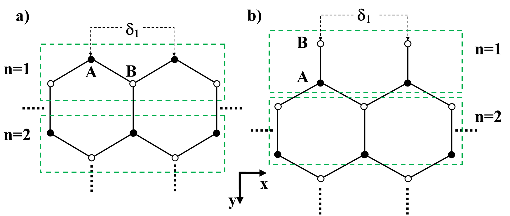
Figure 1: (Color online) Squematics of the a) zig-zag and b) bearded boundaries on the honeycomb lattice. The sub-lattices are labeled by $A$ and $B$. The external on-site potential $\delta_{1}$ is applied at the outermost sites. Here, $n$ is a index row along the $y$ direction perpendicular to the boundary.

II.2 Effective Hamiltonian for the edge states

The Harper’s equation, Eq. (3), can be simplified if we assume a decaying Bloch wavefunction in the $y$ direction of the form, $\psi_{l,n}=z^{n}\psi_{l}$, where $l$ labels each sublattice and the Bloch phase factor $z$ a complex number Ćelić et al. (1996); Pavkov et al. (2001). The effective Hamiltonian for the edge state can be written with the decaying wavefunction as $H_{ef}\psi_{l,n}=\varepsilon\psi_{l,n}$, where

$$H_{ef}=\left[\begin{array}[]{cc}3+J_{3}-J_{4}\Delta&-w\left(J_{1}+J_{2}z^{-1}\right)\\ -w^{-1}\left(J_{1}+J_{2}z\right)&3-J_{3}+J_{4}\Delta\end{array}\right],$$ (4)

and $\Delta=z+z^{-1}$. In the above equation, the factor $w$ takes into account the bearded $(w=z)$ and zig-zag $(w=1)$ boundaries. The non-trivial solution for the eigenstates of $H_{ef}$ gives rise to the secular equation

$$J_{4}^{2}\Delta{}^{2}-\left(2J_{3}J_{4}-J_{1}J_{2}\right)\Delta-\varepsilon_{r}^{2}+J_{1}^{2}+J_{2}^{2}+J_{3}^{2}=0,$$ (5)

where $\varepsilon_{r}=\varepsilon-3$. Note that such polynomial in $\Delta$ is the same for the both considered boundaries. For a given momentum $k$ and energy $\varepsilon$, the solutions of Eq. (5) are the Bloch phase factors $z_{\nu}$, $\nu=1,..,4$. In particular, for the infinite system, the Fourier transform in the $y$ direction is the solution $z=e^{\pm\frac{3}{2}ik_{y}}$ which corresponds to Bloch extended states. In the case of a lattice with a boundary, the solutions of Eq. (5) satisfying $\left|z_{\nu}\right|=1$ determine the bulk band structure [See. Fig. (2)]. The states with $\left|z_{\nu}\right|\neq 1$ decay/grow exponentially in space, and they can be used to describe the edge states with the appropriate boundary conditions.

The factors $z_{\nu}$ and $z_{\nu}^{-1}$ in the Eq. (5) always appear in pairs. Since we require a decaying (evanescent) wave from the boundary, setting the condition $\left|z_{\nu}\right|<1$ implies that the general solution for the edge states can be written as a linear combination of the form,

$$\psi_{l,n}=c_{1}z_{1}^{n}\psi_{l}^{\left(1\right)}+c_{2}z_{2}^{n}\psi_{l}^{\left(2\right)},$$ (6)

where the coefficients $c_{i}$ are determined by the boundary conditions. In the above equation, $\psi_{l}^{(\nu)}$, $\nu=1,2$, is an eigenvector of $H_{ef}$ corresponding to the $\nu-th$ solution. To obtain the edge state energy spectrum, the wavefunctions, Eq. (6), must satisfy the boundary conditions. This will be described in the following sections.

III boundary conditions and the edge states

In this section, the boundary conditions for both zig-zag and bearded boundaries are obtained. By the secular Eq. (4) and the boundary conditions, we derive the analytical expressions for the edge state energy spectrum and wavefunctions for non-zero DMI. Please refer to the appendix A for the solutions with zero DMI.

III.1 Zig-zag boundary

In our previous workPantaleón and Xian (2017), we derive the equations for the energy and the wavefunctions considering a fixed on-site potential $\delta_{1}=1$, where the edge state energy spectrum and the wavefunctions closely resembles the fermionic graphene. Here, we will just summarize the derivation with the notation in this paper and extending the formalism to arbitrary external on-site potentials.

Due to the open zig-zag boundary, the on-site potential along the boundary is different from that in the bulk. Then, the Harper’s equation, Eq. (3), at $n=1$ must be modified. Considering the missing bonds along the outermost $A$ site, the coupled Harper’s equation at $n=1$ is written as,

$$\left(2-\delta_{1}\right)\psi_{A,1}-J_{1}\psi_{B,1}+f_{A,1} =\varepsilon\psi_{A,1},$$

$$3\psi_{B,1}-\left(J_{1}\psi_{A.1}+J_{2}\psi_{A,2}\right)-f_{B,1} =\varepsilon\psi_{B,1},$$ (7)

where the external on-site potential $\delta_{1}$ is introduced and $f_{l,1}=J_{3}\psi_{l,1}-J_{4}\psi_{l,2}$. In the the above equation, the total energy at each sublattice is given by the on-site contribution (first term), the NN contribution (second term) and the DMI (third term). Contrasting the Eq. (3) and Eq. (7), we obtain the zig-zag boundary conditions

$$\left(1-\delta_{1}\right)\psi_{A,1}-J_{4}\psi_{A,0} =0,$$ (8)

$$\psi_{B,0} =0,$$

for the edge state wavefunctions in Eq. (6). Unlike the equivalent fermionic modelDoh and Jeon (2013) where the wavefunctions of both sub-lattices vanish at $n=0$. The Eq. (8) contains two additional terms; the intrinsic and the external on-site potential. As we will shown in the following sections, such extra terms have important effects. From the Eq. (6) and Eq. (8) the non-trivial solution for the coefficients $c_{i}$ provide us the following self-consistent equation for the edge states,

$$\varepsilon=3+J_{3}-J_{4}\left\{\frac{\left[\left(\delta_{1}-1\right)J_{1}-J_{2}J_{4}\right]\left(z_{1}+z_{2}\right)+\left[J_{2}\left(\delta_{1}-1\right)+J_{1}J_{4}\right]\left(1-z_{1}z_{2}\right)}{\left(\delta_{1}-1\right)J_{1}z_{1}z_{2}-J_{2}J_{4}}\right\},$$ (9)

with $z_{1}$ and $z_{2}$ the two decaying solutions of the Eq. (5). The corresponding edge state wavefunctions are given by

$$\psi_{A,n} = c_{1}\left(z_{1}^{n}-\alpha z_{2}^{n}\right)\psi_{A}^{\left(1\right)},$$

$$\psi_{B,n} = c_{1}\left(z_{1}^{n}-z_{2}^{n}\right)\psi_{B}^{\left(1\right)},$$ (10)

where $c_{1}$ is a normalization term, and

$$\alpha=\frac{\left(1-\delta_{1}\right)z_{1}-J_{4}}{\left(1-\delta_{1}\right)z_{2}-J_{4}},$$ (11)

contains the contribution of the external on-site potential in the wavefunction. For a given momentum $k$, external potential $\delta_{1}$ and non-zero DMI, the Eq. (9) is an implicit equation for the energy $\varepsilon$ and can be solved numerically. The Eq. (5), Eq. (9) and Eq. (10) provide us a full description for the edge states energy spectrum and wavefunctions, which will be described in the Sec. IV.

III.2 Bearded boundary

Similar to the zig-zag case, by modifying the Harper’s equation at $n=1$ to take into account the missing sites, the boundary conditions for the wavefunctions in Eq. (6) are given by

$$\left(2-\delta_{1}\right)\psi_{B,1}+J_{4}\psi_{B,0} =0,$$ (12)

$$\psi_{A,0} =0.$$

From the Eq. (6) and Eq. (12) the non-trivial solution for the coefficients $c_{i}$ can also be obtained. However, by a closer inspection of the boundary conditions and the Harper’s equation, we found that the simple replacements: $J_{1}\rightarrow J_{2}$, $J_{2}\rightarrow J_{1}$, $J_{3}\rightarrow-J_{3}$, $J_{4}\rightarrow-J_{4}$ and $\delta_{1}\rightarrow\delta_{1}+1$ in the Eq. (9), provide us the required self-consistent equation for the edge state energy spectrum. The wavefunctions satisfying the boundary conditions, Eq. (12), are given by

$$\psi_{A,n} = c_{1}\left(z_{1}^{n}-z_{2}^{n}\right)\psi_{A}^{\left(1\right)},$$

$$\psi_{B,n} = c_{1}\left(z_{1}^{n}-\alpha^{\prime}z_{2}^{n}\right)\psi_{B}^{\left(1\right)},$$ (13)

where $c_{1}$ is a normalization term and

$$\alpha^{\prime}=\frac{\left(2-\delta_{1}\right)z_{1}+J_{4}}{\left(2-\delta_{1}\right)z_{2}+J_{4}}.$$ (14)

The Eq. (5) and the self-consistent equation obtained by the Eq. (12) and the Eq. (13) provide us a full description for the edge state energy spectrum and wavefunctions. For an arbitrary external on-site potential and zero DMI, the $k-$dependence of $\varepsilon(k)$ and the explicit solutions for the decaying $z$ factors are obtained in the appendix A.

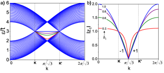
Figure 2: (Color online) a) Edge state dispersion relations induced by $\delta_{1}$ at the zig-zag open boundary are shown for $\delta_{1}=0.2,\,0.6,\,0.8$ and $1.0$ (from the curved to the flat band). For $\delta_{1}=0$ there are not edge states. The blue region is the bulk continuum where all the factors $\left|z_{\upsilon}\right|=1$ in Eq. (5). b) Modulus of the decaying factors for the corresponding edge states, here $\pm 1$ is the sign of $z_{1}$.

IV energy spectrum and wavefunctions

IV.1 Zero DMI

In a fermionic lattice with a boundary, it is well known that there are flat edge states connecting the two Dirac points, $\boldsymbol{K}\rightarrow\boldsymbol{K^{\prime}}$, in a lattice with a zig-zag boundaryFujita et al. (1996), where in a lattice with a bearded boundary Klein (1994), the flat edge state is connecting the complementary region, $\boldsymbol{K^{\prime}}\rightarrow\boldsymbol{K}$. In the equivalent bosonic models, some differences are expected due to the contribution of the on-site interactions along the boundary sites.

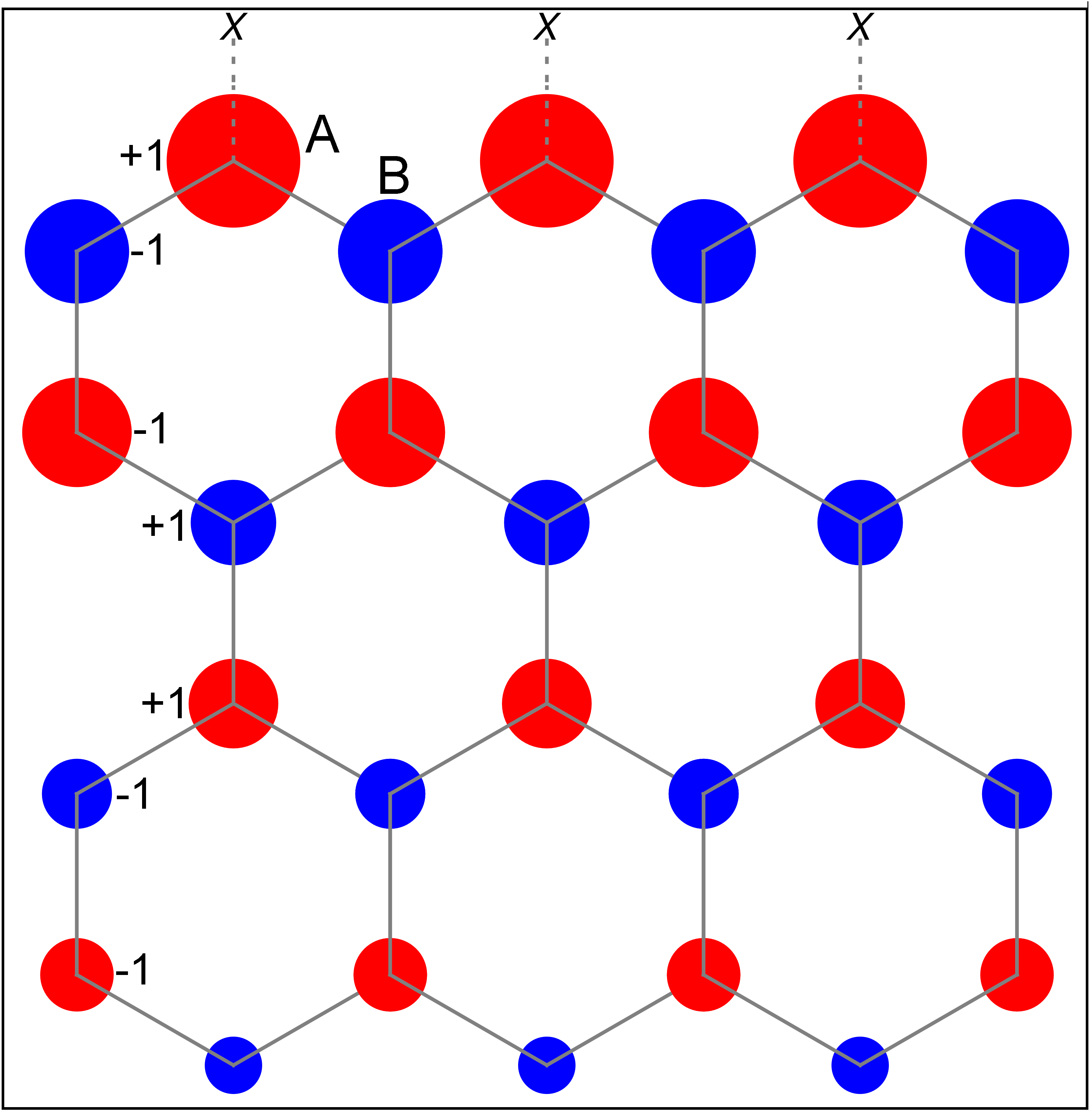
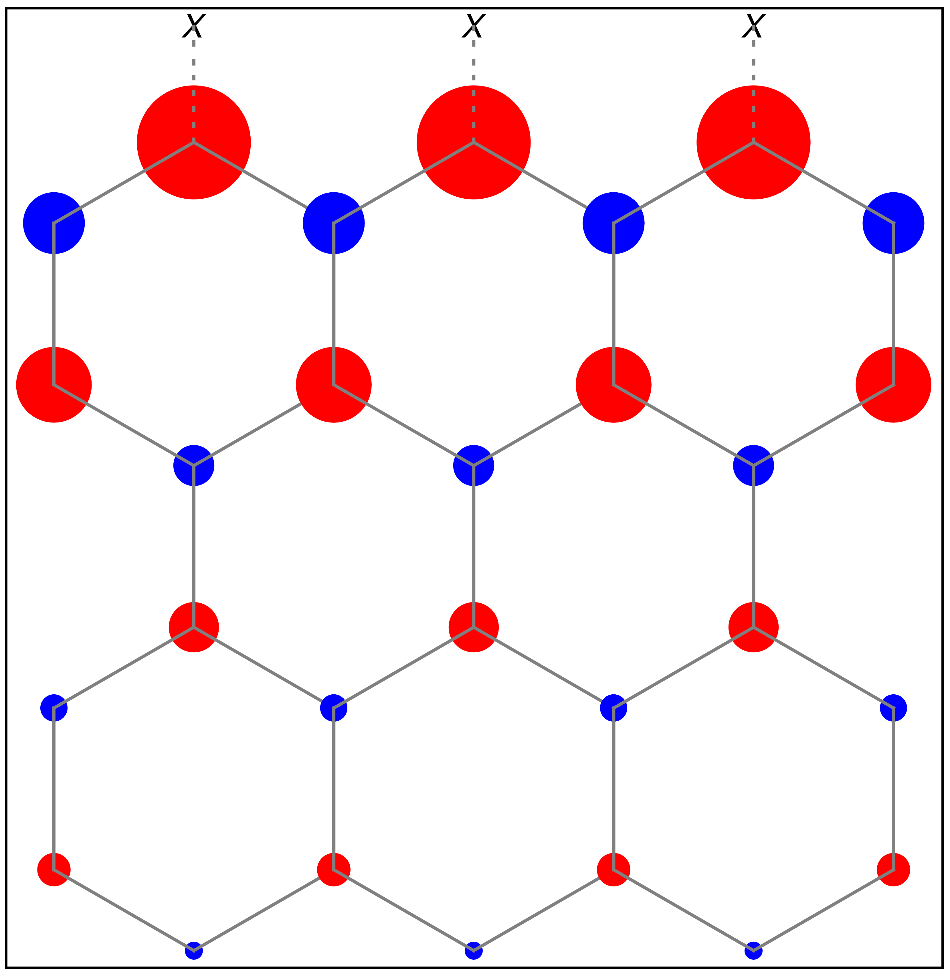
Figure 3: (Color online) Spin density profile for $k=1.41$ and external on-site potential a) $\delta_{1}=0.2$ and b) $\delta_{1}=0.4$. For clarity, the magnitudes on the edge are held constant. The magnitudes of the spin density are proportional to the radius of each circle with a phase given by $e^{in\theta_{l}}=\pm 1$.

IV.1.1 Zig-zag boundary

For a zig-zag boundary, in the absence of external on-site potentials and zero DMI, the obtained physical solutions are bulk states with $z^{2}=1$ and $\varepsilon=2\pm\left|J_{1}\right|$. As shown in the Fig. (1a), the outermost $A$ site has two nearest neighbors and the missing bond generates an attractive potential which acts as an effective defect which surprisingly does not allow the formation of edge states. To induce a Tamm-like edge state, the effective defect is strengthened by turning on the external on-site potential, $\delta_{1}$. In the Fig. (2) the energy spectra and the decaying factors of the induced edge states are shown for different values of $\delta_{1}$. As the external on-site potential is increasing $(\delta_{1}\rightarrow 1)$, the branch becomes flatter [Fig. (2a)] and from the edge state wavefunctions,

$$\left(\begin{array}[]{c}\psi_{A,n}\\ \psi_{B,n}\end{array}\right)=z^{n}\left(\begin{array}[]{c}z^{-1}\\ \frac{1-\delta_{1}}{J_{2}}\end{array}\right),$$ (15)

the magnon density is increasingly localized in a single lattice [See Fig. (3)]. In the above equation, the decaying factor $z$ is a real number. For a wide ribbonHatsugai (1993a, b), the edge state energy spectra is double degenerated and since the magnon velocity is the slope of the energy spectrum, Fig. (2), the magnons are moving in the same direction at opposite edges, Fig. (4a). Here, as $\delta_{1}$ is increased the slope is reduced until $\delta_{1}=1$ where the edge state becomes non-dispersive.

If the external on-site potential is increased, in addition to the shape, the number of edge states can be modified. Depending on the external on-site potential strength, a zig-zag termination can have two edge states at each boundary. In the decaying factor diagram, Fig. (5a), each edge state has a corresponding, $z_{1}$ or $z_{1}^{\prime}$, decaying factor. For $0<\delta_{1}<2$, there is a single decaying factor between the Dirac points [see also Fig. (2)] and from the Eq. (15) it is straightforward to show that the edge state in this region is mainly localized at the $A$ sublattice. For $\delta_{1}>2$, there are two edge states, the first one, corresponding to $z_{1}^{\prime}$, is defined over all the Brillouin zone with energy spectra over the bulk bands (due to the strong external on-site potential). The second edge state, corresponding to $z_{1}$, is defined in the region $\boldsymbol{K}>k>\boldsymbol{K^{\prime}}$ as in the bearded graphene. Such edge state has a magnon density mainly localized at the $B$ sublattice with energy spectrum between the Bulk bands. If the external on-site potential is stronger, $\delta_{1}\gg 2$, the system effectively shows the band structure of a bearded termination plus a high energy Tamm-like edge state. Moreover, as we mentioned before, in absence of external on-site potential there are not edge states. However, for $\delta=2$, there are not edge states either. This can be observed in the diagram, Fig. (5a), where at such value, $\left|z_{1}\right|=\left|z_{1}^{\prime}\right|=1$ for all values of $k$. At the transition lines (dashed) the modulus of the decaying factors reaches the unity and the edge states are indistinguishable from the bulk bands.

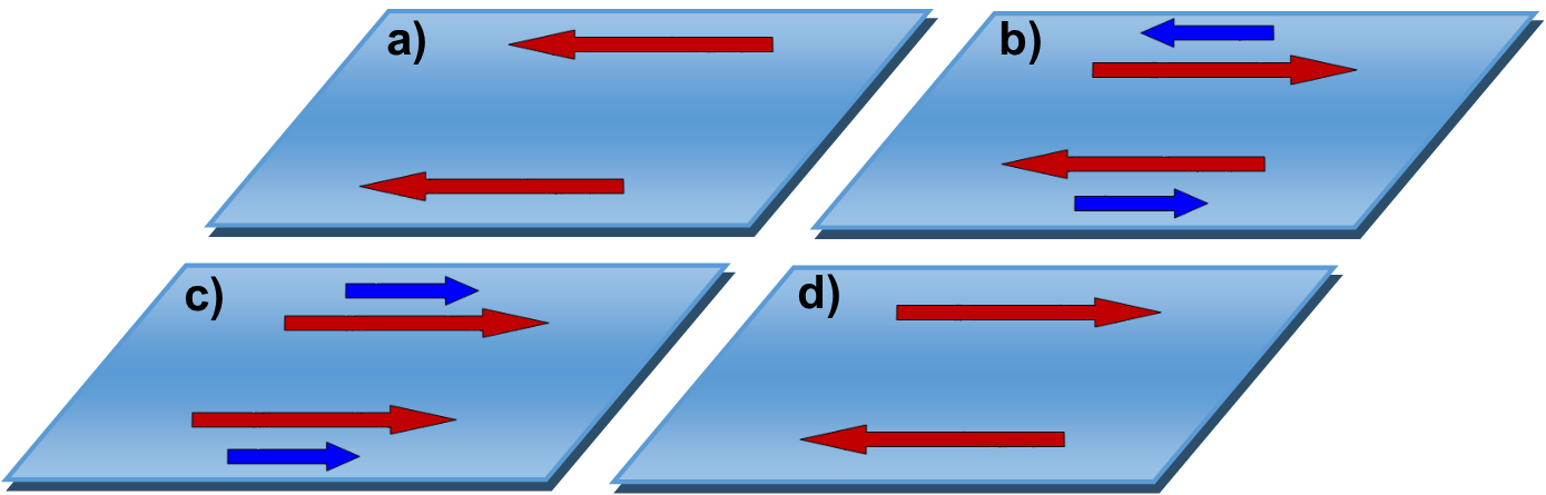
Figure 4: (Color online) Schematic illustrations of the edge states propagation with the same momentum $k$. The arrows represent the edge magnon velocity which depends on the external on-site potential and the DMI strength. Each figure corresponds to a) single edge magnon propagating at each boundary in the same direction, b) two edge magnons with different velocities moving in opposite directions at each boundary, c) two edge states moving in the same direction at the same boundary and d) chiral edge states.

On the other hand, it is well known that the magnon excitations in a ferromagnetic lattice can be viewed as a synchronic precession of the spin vectors. Therefore, the sign of the wavefunction, Eq. (15), can be related with the spin precession in successive, $n$, rows and the modulus with the radius of precession which decrease as $n$ increases. If we write the phase of the wavefunction as $e^{in\theta_{l}}=sgn(\psi_{l,n})$, then, for a given $k$ and $0<\delta_{1}<2$, the synchronic precession of the spins in successive $n$ rows is in anti-phase ($\theta_{l}=\pi$, optic-like) if $k<k_{o}$ and in-phase ($\theta_{l}=0$, acoustic-like) if $k>k_{o}$, here, $k_{0}=\pi/\sqrt{3}$ is the transition point. Furthermore, at the same $n$, the spins at different sub-lattices are precessing in anti-phase for $k<k_{o}$ and in-phase for $k>k_{o}$ [See Fig. (3a)]. At the transition point $k_{0}$, the edge state energy is $\varepsilon_{0}=2+\delta_{1}$ and the decaying factor is zero, Fig. (2b). Hence, by the Eq. (15), the magnon is completely localized at the edge site, independently of the external on-site potential strength.

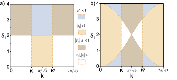
Figure 5: (Color online) Decaying factor diagram for the edge states in a honeycomb lattice with a) zig-zag and b) bearded termination and zero DMI. The number of decaying factors with $\left|z\right|<1$ is the number of edge states in the corresponding region. The (dashed) lines dividing each region are the points where both decaying factors reach the unity.

IV.1.2 Bearded boundary

We now consider a bearded termination. As shown in the Fig. (1b), the outermost site has two missing bonds and the effective defect is stronger than the corresponding to a zig-zag boundary. On the contrary of the fermionic equivalent, the on-site terms provided by the Eq. (1) change substantially the edge state band structure. This is shown in the Fig. (6a), where for $\delta_{1}=0$ there are two edge state energy bands, Eq. (22), the first one between the Dirac points (dot-dashed, black line) and the second one below the lower bulk bands (dashed, black line). Such edge states are defined in a region in $k$ completely different to their fermionic equivalentKlein (1994); Jaskólski et al. (2011). As shown in the Fig. (6b), the edge state below the bulk bands is defined over all the Brillouin zone, except at $k=0,2\pi\sqrt{3}$, where the decaying factor reaches the unity and the edge state is indistinguishable from the bulk bands. Excluding those merging points, the edge state wavefunction with a real decaying factor $z$,

$$\left(\begin{array}[]{c}\psi_{A,n}\\ \psi_{B,n}\end{array}\right)=z^{n}\left(\begin{array}[]{c}\frac{2-\delta_{1}}{J_{1}}\\ z^{-1}\end{array}\right),$$ (16)

reveals that the low energy edge state is strongly localized along the boundary $B$-sites. In the above equation, $z=z_{1}^{\prime}$ , for the edge state below the lower bulk bands and $z=z_{1}$ for the edge state between the Dirac points [see Fig. (5)]. In the Fig. (6c) and Fig. (6d), we plot the magnon density, $\left|\psi_{l,n}\right|^{2}$ for both edge states at different momentum. Note that the edge states are localized in different sub-lattices.

Some interesting features about these edge states are in order here. From the Fig. (6a), for $\delta_{1}=0$ the slope the edge state energy spectra is positive if $k<k_{0}$ and negative if $k>k_{0}$. For a wide ribbon, each edge band is doubly degenerated, hence, the magnons are moving in the same direction (with different energy) at each boundary, Fig. (4c). The fact that both edge states are strongly localized in different sub-lattices can be explained if we consider the edge by itself a defect. By a closer inspection of the wavefunctions, Eq. (16), the edge state below the lower bulk bands is mainly localized along the boundary $B$ sites due to the strong attractive potential due to the missing bonds. The edge state between the bulk bands is mainly localized along the $A$ sublattice due to the presence of the outermost $B$ site. In consequence, the outermost $B$ site plays a double role; acts as an effective defect to host a low energy edge state and contributes to the formation of the edge state between the Dirac points.

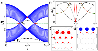
Figure 6: (Color online) a) Bulk (blue region) and edge state energy spectra for $\delta_{1}=0$, (black, dashed and dot-dashed lines), $\delta_{1}=1.8$ (red, continuous lines) and $\delta_{1}=2$ (green, dotted lines). In b) we show their corresponding decaying factors. The magnon density profile is shown for the edge states with $\delta_{1}=0$ at c) $k=1.40$ and d) $k=0.96$. Here, the magnitudes of the spin density are proportional to the radius of each circle with a phase given by $e^{in\theta_{l}}=\pm 1$.

The number of edge states is determined by the number of solutions of the Eq. (19) with modulus lower than one and the edge state dispersion can be tuned in all the Brillouin zone with small changes of the external on-site potential. This can be observed in the decaying factor diagram, Fig. (5b), where the dashed lines separate the regions in which each edge state is defined. In the region, $0\leq\delta_{1}<1$, there are always two edge states (for $z_{1}^{\prime}$ and $z_{1}$). If $\delta_{1}=0$, the first edge state is defined over all the Brillouin zone, $\left|z_{1}^{\prime}\right|<1$, and the second one between the Dirac points, $\left|z_{1}\right|<1$. As $\delta_{1}$ is increased both edge states gradually merge with the bulk bands. For $\delta_{1}=2$, there is a single edge state with a momentum in the region, $\boldsymbol{K}>k>\boldsymbol{K^{\prime}}$. This edge state is the flat band in Fig. (6a), (dotted, green line) where the energy spectra closely resembles the fermionic graphene. If the external on-site potential is increased, $\delta_{1}\gg 2$, the hopping between sites at $n=1$ is almost suppressed and the system effectively will show the band structure of a zig-zag termination plus and a high energy Tamm-like edge state along the boundary sites.

Another important characteristic provided by the explicit form of the wavefunction, Eq. (16) is the phase of the spin precession in successive rows. As discussed in the previous section, the sign of the decaying factor determines if the phase of the edge state is optic-like or acoustic-like. As is described in the appendix A, there are two decaying factors and their sign reveals that the behavior of the phase in successive rows is different in both edge states. In particular for $\delta_{1}=0$, the decaying factor of the edge state connecting the Dirac points is negative if $k<k_{0}$, then, the spin precession in successive lattice sites is in anti-phase (optic-like). However, the decaying factor of the edge state below the lower bulk bands is positive, if $k<k_{0}$, and the spins in two successive rows are in-phase (acoustic-like). This provide us two ways to distinguish these edge states, by their energy and their phase difference in successive rows.

Experimentally, the first observation of edge states in a honeycomb lattice with bearded boundaries were achieved in optical lattices Plotnik et al. (2014). Apart from the typical band structure, additional edge states were observed near the Van Hoove singularities. As is shown in the Fig. (6a) for our model, similar edge states are obtained for an external on-site potential of $\delta_{1}=1.8$. Here a nearly flat band plus two highly dispersive edge states near the Van Hoove singularities (continuous, red lines) are obtained. As in the reference Plotnik et al. (2014), the origin of such edge states is also related to the effective defect generated by the on-site potential along the boundary sites. In our model, the external on-site potential is introduced at the outermost sites with fixed hopping terms. However, as in the case of an square latticeDe Wames and Wolfram (1969); Hoffmann (1973), similar physics can be obtained by a renormalization of the hopping terms along the boundary sites.

IV.2 Non-zero DMI

A non-zero DMI breaks the lattice inversion symmetry and a non-trivial gap is induced in the spin-wave excitation spectra. By a topological approach with the wavefunctions for the infinite system, the Chern number predicts a pair of counter propagating modesOwerre (2016a) along the boundary of the finite system. However, the topological approach does not provide the detailed properties of the edge states and also does not take into account the on-site potential along the boundary sites, which, as we will shown in this section, has important effects in the edge state band structure.

IV.2.1 Zig-zag boundary

We first consider a zig-zag boundary. The energy bands are obtained by the solutions of the self-consistent Eq. (9) with the decaying factors provided by the Eq. (5). In the Fig. (7a) we show the energy bands for a DMI strength of $D=0.1J$. The blue regions correspond to the bulk spectra where all the factors, $\left|z_{\nu}\right|=1$. The bands which transverse the gap are the spectra of the edge states for different values of $\delta_{1}$. By completeness, we also include the energy spectra for the edge state at the opposite edge (at large $n$), without external on-site potential. On the contrary to the predicted by a topological approach Owerre (2016a); Kim et al. (2016), the edge state is not connecting the regions near the Dirac points. As is shown in the Fig. (7a), for $\delta_{1}=0$ (red, continuous line) the intrinsic on-site potential along the boundary pull the edge state within the bulk gap to a lower energy region, just over the lower bulk bands. Furthermore, a new edge state near the Van Hoove singularities is revealed in the band structure. As is shown in the zoomed region, Fig. (7b), around $k_{0}$ there are two edge states (at each boundary), over and below the lower bulk band. The edge state over the bulk bands has a topological origin and the edge state below is a Tamm-like edge state.

In general, the edge states depend on two decaying factors, Eq. (10). In the Fig. (7c) their typical behavior can be observed; if we move away from $k_{0}$, while one factor decreases to zero the another one approaches to a critical value (merging point) where it reaches the unity. In this situation, one component of the edge state wavefunction becomes an extending wave (bulk wave) and the edge state is indistinguishable from the bulk bands. However, for the edge state below the lower bulk bands, (7d), in the region $k>k_{0}$, while one decaying factor reaches the unity the second one has enough strength to modified the bulk band structure [arrows in Fig. (7b) and Fig. (7d)], in this situation the edge state has energy within the continuumZhang et al. (2012); Longhi and Della Valle (2013). For $\delta_{1}=0$ (and $D\neq 0$), the edge band within the bulk gap has a negative slope while the novel edge band below the lower bulk band has a positive slope. Therefore, the magnons are moving in opposite directions at the same boundary, Fig. (4b). If the external on-site potential is slightly increased, the Tamm-like edge magnon merges with the bulk and the magnon propagation will be like in the Fig. (4d).

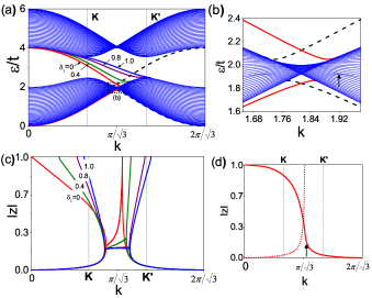
Figure 7: (Color online) a) Energy spectrum of a zig-zag honeycomb lattice for $D=0.1\,J$. The lines connecting the upper and lower bulk bands are the edge states for different values of $\delta_{1}$, the dashed (black) lines are the edge states at the opposite edge. As shown in b) for $\delta_{1}=0$ there are additional edge states below the lower bulk bands, dashed square in a). In c) the decaying factors of the corresponding edge states in a) is shown. d) Decaying factors $\left(\delta_{1}=0\right)$ of the edge state below the lower bulk band in a) and b). The energy spectra in b) reveals an edge state with energy within the bulk bands (black arrow), the magnitude of its corresponding decaying factor is given by the arrow in d)

As is shown in the Fig. (7a) as the external on-site potential is increasing, the slope of the energy spectra decreases. In particular, for $\delta_{1}=1$ (uniform case) the energy spectra closely resembles the fermionic graphene with merging points near the Dirac points and with the magnons moving in opposite directions at different boundaries, Fig. (4d). In the Fig. (7c) the modulus of the decaying factors is shown for different values of the external on-site potential. Here, as $\delta_{1}$ is increased, the merging points approaches by the left to the $\boldsymbol{K}$ and $\boldsymbol{K}^{\prime}$ points and the asymmetry around $k_{0}$ is reduced. In the finite region [Fig. (7c)] around $k_{0}$, we have $\left|z_{1}\right|=\left|z_{2}\right|$ and from the Eq. (5) is evident that the decaying factors are complex conjugates to each other. At certain momentum both decaying factors become real and they are not longer identical and, as we mentioned before, while one factor increases the another one decreases. The region around $k_{0}$, where the edge states are complex conjugates to each other, is defined for a non-zero DMI and is located within the bulk gap. Its boundaries in the $k$ space are given by the discriminant of Eq. (5) and is independent of the boundary conditions. If the spectrum of an edge state crosses this region, their corresponding wavefunction becomes complex.

IV.2.2 Bearded boundary

We now consider a bearded termination with a non-zero DMI and arbitrary external on-site potential. The solutions can be obtained by the self-consistent equation provided by the Eq. (12) and the wavefunctions with the Eq. (13). As is shown in the Fig. (8) for $\delta_{1}=0$, there is an edge state crossing the gap (red, continuous line) and an edge state below the lower bulk bands (purple, continuous line). Note that the non-zero DMI changes the magnon velocity. In fact, the edge state within the gap has a negative slope except near the $\boldsymbol{K}$ point where is almost flat. The edge state energy spectrum below the lower bulk bands has a maximum point where its slope changes. Before such point and out from the almost flat region, the propagation is like in the Fig. (4b) where, for a fixed momentum and at the same boundary, the magnons are moving in different directions. On the other hand, as is shown in the Fig. (8a), to the right of the $\boldsymbol{K}^{\prime}$ point, there are two edge bands with negative slope (red and purple continuous lines) and a single edge band with negative slope at the opposite boundary (green, dot-dot-dashed line), hence the magnons are moving in the same direction at both edges.

The effective defect due to the missing bonds is strong in the bearded boundary, where the edge state energy spectra are distinct to their fermionic equivalent. As shown in the Fig. (8b) the edge state within the bulk gap (red, continuous line) is defined in a region to the right of the $\boldsymbol{K}$ point. The edge state below the lower bulk bands is defined over the whole Brillouin zone and since its origin is due to the effective defect discussed in the previous section, it can be shown that is nearly insensitive to small changes in the DMI strength. In the Fig. (8c) the decaying factors modulus for this edge state are shown. The curves are almost symmetric around $k_{0}$ and since the decaying factors are real, the wavefunction decays exponentially to the inner bulk sites Doh and Jeon (2013); Pantaleón and Xian (2017).

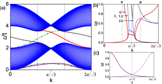
Figure 8: (Color online) a) Energy spectrum of a bearded honeycomb lattice. The blue region is the gapped bulk spectra with $D=0.1J$. For $\delta_{1}=0$, the continuous (red and purple) lines are the edge states. By completeness, we also include the edge states at the opposite edge, dot-dot-dashed (green) lines. For $\delta_{1}=2$ there is a single edge state (black, dotted line). In b) we plot the modulus of the two decaying factors for the edge state connecting the bulk bands at different values of $\delta_{1}$. In c) the decaying factors for $\delta_{1}=0$ are shown for the edge state below the lower bulk bands.

As discussed in the previous section, as we move away from $k_{0}$, one decaying factor approaches to the unity while the another one decreases. Note that the Fig. (8b) is similar to the Fig. (7b) except that the plots are tilted to opposite sides. Here, as the external on-site potential is increased, the merging points approach to $k_{0}$. In particular for $\delta_{1}=2$, the edge state has an energy spectrum connecting the Dirac points (black, dotted line in Fig. (8a)). However, in contrast with their fermionic equivalent, around $k_{0}$ (Van Hoove singularity) there is an small region in which a high dispersive (and almost indistinguishable) edge state is also defined, (black-dotted line in Fig. (8a) and (8b)). If $\delta_{1}\gg 2$, as in the case for $D=0$, the system effectively will show the band structure of a zig-zag termination plus and a high energy Tamm-like edge state.

V Concluding remarks

Recently, it has been shown that a system of two-interacting bosons in a honeycomb lattice satisfy the Hamiltonian given in Eq. (1) in the limit of strong interaction and with renormalized parametersSalerno et al. (2017). In particular, for a bearded boundary, the two-particle system (doublon) behaves like a single particle and the edge state energy spectra in the Fig. (8) is obtained. In this model, an isotropic coupling constant $J(>0)$ is considered over the whole semi-infinite lattice. Due to the on-site contributions in the Hamiltonian, Eq. (1), the missing bonds reduce of the on-site energy along the boundary sites. Since the on-site contribution is the number of nearest-neighbors, the external on-site potential $\delta_{1}$ is introduced as an extra bond which does not have any effect in the hopping parameters. The model presented in this paper has the advantage that the boundary conditions can be easily modified without modify the Harper’s equation. For example, instead of introduce an extra bond, a renormalization of the hopping parameters along the boundary can also be introduced by allowing to the exchange parameters to deviate from the bulk values. Similarly to the model for the surface spin waves in an square latticeDe Wames and Wolfram (1969), we can consider different coupling constants along the boundary sites. However, such modifications does not changes the physics of this problem where the edge by itself is considered as an effective defect. As we mentioned before, such effective defect is due to the missing bonds along the boundary sites and is a characteristic of the bosonic lattices, consequently, the physical systems modeled by a bosonic Hamiltonian, Eq. (1), may show edge states naturally or through the application of small external on-site potentials.

The interesting properties of the honeycomb lattice may be experimentally accessible through engineered spin structures on metallic surfacesBanerjee et al. (2016), using ultra-cold bosonic atoms trapped in honeycomb optical lattice Vasić et al. (2015), photonic latticesPolini et al. (2013); Bellec et al. (2014) and so forth. Therefore, the distribution of the edge magnons, the spin-density and their dependence with the DMI strength and external on-site potentials presented in this paper could be useful for experiments in small sized mono-layers, thin film magnets or artificial lattices.

VI Conclusions

We have studied the on-site potential effects in the magnon edge states in a honeycomb ferromagnetic lattice with zig-zag and bearded boundaries. For zero DMI, the connection of the formation of the Tamm-like edge states with the effective defect due to the on-site potential along the outermost sites has been elucidated. For non-zero DMI, we found that the edge state energy spectra is modified due to the missing bonds along the boundary sites and their distribution in the momentum space is different to that predicted by a topological approach. For both zig-zag and bearded boundaries and for zero and non-zero DMI, the edge state properties are discussed and Tamm-like edge states have been revealed. Nevertheless, if these edge states can also be predicted by a topological approach is still an open question. We found that the Tamm-like and the topologically protected edge states are tunable by modifying the external on-site potential and the DMI. Furthermore, analytical expressions for the edge state energy spectrum and their corresponding wavefunctions are obtained. We believe that our results may explain the unconventional edge states recently found in optical Plotnik et al. (2014); Milićević et al. (2017) and acoustic Ni et al. (2017) lattices and motivate new experiments in topological bosonic insulators.

Note added. After completion of this work, a related work have appeared in which the magnon edge states in a honeycomb ferromagnet are also discussed Pershoguba et al. (2017). The analytical solutions and the edge state properties, however, are not discussed.

Appendix A Analytical solutions for $D=0$

In this appendix, we derive the edge state energy spectrum and wavefunctions for a semi-infinite ferromagnetic honeycomb lattice with a bearded boundary, in absence of DMI and with an arbitrary external on-site potential $\delta_{1}$. From the Eq. (5) for $D=0$, the characteristic equation of $H_{ef}$, Eq. (4 ), is given by,

$$\left(3-\varepsilon\right)^{2}-J_{1}^{2}-J_{2}^{2}-J_{1}J_{2}\left(z+z^{-1}\right)=0.$$ (17)

For a fixed $k$, the above equation relates the decaying factor $z_{1}$ with the energy $\varepsilon$. However, an additional equation provided by the boundary conditions is required. From the Harper’s equation, Eq. (3), with the replacements $J_{1}\rightarrow J_{2}$ , $J_{2}\rightarrow J_{1}$ and taking into account the missing bonds, the additional equation for the edge state at $n=1$ is written as,

$$\left(3-\varepsilon\right)\left(1+\delta_{1}-\varepsilon\right)-J_{1}J_{2}z+J_{2}^{2}=0.$$ (18)

Here, both Eq. (17) and Eq. (18) provide us a complete set of equations for the decaying factor and the energy spectrum. Therefore, for an arbitrary external on-site potential, $\delta_{1}$, the decaying factor satisfy,

$$az_{1}^{2}+bz_{1}+c=0,$$ (19)

where, $a=\left(-2+\delta_{1}\right)^{2}J_{2}$, $b=J_{1}\left[\left(-2+\delta_{1}\right)^{2}-J_{1}^{2}\right]$ and $c=-J_{1}^{2}J_{2}$. Explicitly,

$$z_{1}=\frac{-\left(\delta_{b}^{2}-J_{1}^{2}\right)^{2}J_{1}\pm\left|J_{1}\right|\sqrt{\left(\delta_{b}^{2}-J_{1}^{2}\right)^{2}+4\delta_{b}^{2}}}{2\delta_{b}^{2}},$$ (20)

where $\delta_{b}=-2+\delta_{1}$ and $J_{2}=1$. On the other hand, the edge state energy spectrum satisfy,

$$a_{1}\varepsilon_{r}^{2}+b_{1}\varepsilon_{r}+c_{1}=0,$$ (21)

where, $\varepsilon_{r}=(\varepsilon-3)-(-2+\delta_{1})$, $a_{1}=(-2+\delta_{1})J_{1}$, $b_{1}=b$ and $c_{1}=-(-2+\delta_{1})J_{1}J_{2}^{2}$. The edge state energy spectra have two solutions given by,

$$\varepsilon=\frac{6\delta_{b}+\delta_{b}^{2}+J_{1}^{2}\pm sgn\left(J_{1}\right)\sqrt{\left(\delta_{b}^{2}-J_{1}^{2}\right)^{2}+4\delta_{b}^{2}}}{2\delta_{b}}.$$ (22)

From the above equation and by a closer inspection of the decaying factors, Eq. (20) two edge states can be defined. The wavefunction satisfying the boundary condition,

$$\left(2-\delta_{1}\right)\psi_{B,1}-J_{1}\psi_{A,0}=0,$$ (23)

can be written as,

$$\psi_{l,n}=z_{1}^{n}\left(\begin{array}[]{c}\frac{2-\delta_{1}}{J_{1}}\\ z_{1}^{-1}\end{array}\right),$$ (24)

where the decaying factor $z_{1}$ is given the by Eq. (20). At the point $k_{0}=\pi/\sqrt{3}$, the edge states are completely localized at the boundary sites with energy,

$$\varepsilon_{k_{0}}=\frac{1}{2}\left(6+\delta_{b}\right)\pm\sqrt{4+\delta_{b}}.$$ (25)

In particular, for $\delta_{1}=2$ the Eq. (19) provide us a single decaying factor, $z_{1}=-J_{2}/J_{1}$ and the Eq. (21) a single solution $\varepsilon=3$, which is a flat band similar to the fermionic graphene. Following the same procedure, the analytical form of the decaying factor and the edge state energy spectrum for a zig-zag boundary can also be obtained.

References

- Tamm (1932) I. Tamm, Phys. Z. Sov. Union 1, 733 (1932).
- Shockley (1939) W. Shockley, Phys. Rev. 56, 317 (1939).
- Hasan and Kane (2010) M. Z. Hasan and C. L. Kane, Rev. Mod. Phys. 82, 3045 (2010).
- Hatsugai (1993a) Y. Hatsugai, Phys. Rev. B 48, 11851 (1993a).
- Hatsugai (1993b) Y. Hatsugai, Phys. Rev. Lett. 71, 3697 (1993b).
- Delplace et al. (2011) P. Delplace, D. Ullmo, and G. Montambaux, Phys. Rev. B 84, 195452 (2011).
- Malki and Uhrig (2017) M. Malki and G. S. Uhrig, Phys. Rev. B 95, 235118 (2017).
- Matsumoto and Murakami (2011) R. Matsumoto and S. Murakami, Phys. Rev. B 84, 184406 (2011).
- Zhang et al. (2013) L. Zhang, J. Ren, J.-S. Wang, and B. Li, Phys. Rev. B 87, 144101 (2013).
- Mook et al. (2014) A. Mook, J. Henk, and I. Mertig, Phys. Rev. B 90, 024412 (2014).
- Owerre (2016a) S. A. Owerre, J. Phys. Condens. Matter 28, 386001 (2016a).
- Bloch (1930) F. Bloch, Z. Phys. 61, 206 (1930).
- Holstein and Primakoff (1940) T. Holstein and H. Primakoff, Phys. Rev. 58, 1098 (1940).
- Büttner et al. (2000) O. Büttner, M. Bauer, A. Rueff, S. Demokritov, B. Hillebrands, A. Slavin, M. Kostylev, and B. Kalinikos, Ultrasonics 38, 443 (2000).
- Kajiwara et al. (2010) Y. Kajiwara, K. Harii, S. Takahashi, J. Ohe, K. Uchida, M. Mizuguchi, H. Umezawa, H. Kawai, K. Ando, K. Takanashi, S. Maekawa, and E. Saitoh, Nature 464, 262 (2010).
- Pulizzi (2012) F. Pulizzi, Nat. Mater. 11, 367 (2012).
- Kruglyak and Hicken (2006) V. Kruglyak and R. Hicken, J. Magn. Magn. Mater. 306, 191 (2006).
- Kruglyak et al. (2010) V. V. Kruglyak, S. O. Demokritov, and D. Grundler, J. Phys. D. Appl. Phys. 43, 264001 (2010).
- Chumak et al. (2015) A. V. Chumak, V. I. Vasyuchka, A. A. Serga, and B. Hillebrands, Nat. Phys. 11, 453 (2015).
- Chumak and Schultheiss (2017) A. V. Chumak and H. Schultheiss, J. Phys. D. Appl. Phys. 50, 300201 (2017).
- Onose et al. (2010) Y. Onose, T. Ideue, H. Katsura, Y. Shiomi, N. Nagaosa, and Y. Tokura, Science (80-. ). 329, 297 (2010).
- Chisnell et al. (2015) R. Chisnell, J. S. Helton, D. E. Freedman, D. K. Singh, R. I. Bewley, D. G. Nocera, and Y. S. Lee, Phys. Rev. Lett. 115, 147201 (2015).
- Madon et al. (2014) B. Madon, D. C. Pham, D. Lacour, A. Anane, R. B. V. Cros, M. Hehn, and J. E. Wegrowe, (2014), arXiv:1412.3723 .
- Tanabe et al. (2016) K. Tanabe, R. Matsumoto, J.-I. Ohe, S. Murakami, T. Moriyama, D. Chiba, K. Kobayashi, and T. Ono, Phys. status solidi 253, 783 (2016).
- Cao et al. (2015) X. Cao, K. Chen, and D. He, J. Phys. Condens. Matter 27, 166003 (2015).
- Kim et al. (2016) S. K. Kim, H. Ochoa, R. Zarzuela, and Y. Tserkovnyak, Phys. Rev. Lett. 117, 227201 (2016).
- Owerre (2016b) S. A. Owerre, J. Appl. Phys. 120, 43903 (2016b).
- Pantaleón and Xian (2017) P. A. Pantaleón and Y. Xian, J. Phys. Condens. Matter 29, 295701 (2017).
- Pantaleón and Xian (2018) P. A. Pantaleón and Y. Xian, Phys. B Condens. Matter 530, 191 (2018).
- De Wames and Wolfram (1969) R. E. De Wames and T. Wolfram, Phys. Rev. 185, 720 (1969).
- Hoffmann (1973) F. Hoffmann, Solid State Commun. 13, 1079 (1973).
- Puszkarski (1973) H. Puszkarski, IEEE Trans. Magn. 9, 22 (1973).
- Plotnik et al. (2014) Y. Plotnik, M. C. Rechtsman, D. Song, M. Heinrich, J. M. Zeuner, S. Nolte, Y. Lumer, N. Malkova, J. Xu, A. Szameit, Z. Chen, and M. Segev, Nat. Mater. 13, 57 (2014).
- Milićević et al. (2017) M. Milićević, T. Ozawa, G. Montambaux, I. Carusotto, E. Galopin, A. Lemaître, L. Le Gratiet, I. Sagnes, J. Bloch, and A. Amo, Phys. Rev. Lett. 118, 107403 (2017).
- Ni et al. (2017) X. Ni, M. A. Gorlach, A. Alu, and A. B. Khanikaev, New J. Phys. 19, 055002 (2017).
- Kane and Mele (2005) C. L. Kane and E. J. Mele, Phys. Rev. Lett. 95, 226801 (2005).
- Haldane (1988) F. D. M. Haldane, Phys. Rev. Lett. 61, 2015 (1988).
- Harper (1955) P. G. Harper, Proc. Phys. Soc. Sect. A 68, 874 (1955).
- Ćelić et al. (1996) A. Ćelić, D. Kapor, M. Škrinjar, and S. Stojanović, Phys. Lett. A 219, 121 (1996).
- Pavkov et al. (2001) M. Pavkov, M. Škrinjar, D. Kapor, M. Pantić, and S. Stojanović, Phys. Lett. A 281, 347 (2001).
- Doh and Jeon (2013) H. Doh and G. S. Jeon, Phys. Rev. B 88, 245115 (2013).
- Fujita et al. (1996) M. Fujita, K. Wakabayashi, K. Nakada, and K. Kusakabe, J. Phys. Soc. Japan 65, 1920 (1996).
- Klein (1994) D. Klein, Chem. Phys. Lett. 217, 261 (1994).
- Jaskólski et al. (2011) W. Jaskólski, A. Ayuela, M. Pelc, H. Santos, and L. Chico, Phys. Rev. B 83, 235424 (2011).
- Zhang et al. (2012) J. M. Zhang, D. Braak, and M. Kollar, Phys. Rev. Lett. 109, 116405 (2012), arXiv:1205.6431 .
- Longhi and Della Valle (2013) S. Longhi and G. Della Valle, J. Phys. Condens. Matter 25, 235601 (2013).
- Salerno et al. (2017) G. Salerno, M. Di Liberto, C. Menotti, and I. Carusotto, (2017), arXiv:1711.01272 .
- Banerjee et al. (2016) S. Banerjee, J. Fransson, A. M. Black-Schaffer, H. Ågren, and A. V. Balatsky, Phys. Rev. B 93, 134502 (2016).
- Vasić et al. (2015) I. Vasić, A. Petrescu, K. Le Hur, and W. Hofstetter, Phys. Rev. B 91, 094502 (2015).
- Polini et al. (2013) M. Polini, F. Guinea, M. Lewenstein, H. C. Manoharan, and V. Pellegrini, Nat. Nanotechnol. 8, 625 (2013).
- Bellec et al. (2014) M. Bellec, U. Kuhl, G. Montambaux, and F. Mortessagne, New J. Phys. 16, 113023 (2014).
- Pershoguba et al. (2017) S. S. Pershoguba, S. Banerjee, J. C. Lashley, J. Park, H. Ågren, G. Aeppli, and A. V. Balatsky, (2017), arXiv:1706.03384 .