Assisted Vacuum Decay by Time Dependent Electric Fields

Abstract

We consider the vacuum decay by electron-positron pair production in spatially homogeneous, time dependent electric fields by means of quantum kinetic equations. Our focus is on the impact of various pulse shapes as envelopes of oscillating fields and the assistance effects in multi-scale fields, which are also seen in photons accompanying the creation and motion of pairs.

1 Introduction

Besides pair (e.g. electron-positron, $e^{+}$$e^{-}$) creation in counter propagating null fields, e.g. by the Breit-Wheeler process, also other purely electromagnetic fields qualify for pair production. An outstanding example is the Schwinger effect originally meaning the instability of a spatially homogeneous, purely electric field with respect to the decay into a state with pairs and a screened electric field schwinger (1) (cf. gelis_schwinger_2016 (2) for a recent review). The pair creation rate $\propto\exp\{-\pi E_{c}/|\vec{E}|\}$ for electric fields $\vec{E}$ attainable presently in mesoscopic laboratory installations is exceedingly small since the Sauter-Schwinger (critical) field strength sauter (3) $E_{c}=m^{2}/|e|=$1.3\text{\times}{10}^{16}\text{\,}\mathrm{V}\mathrm{/}\mathrm{c}\mathrm{m}$$ for electrons/positrons with masses $m$ and charges $\pm e$ is so large (we employ here natural units with $c=\hbar=1$).

An analogous situation of vacuum decay is met in the case, where a spatially homogeneous electric field has a time dependence. The particular case of a periodic field is dealt with in brezin_pair_1970 (4) with the motivation that tightly focused laser beams can provide high field strengths. The superposition of a few laser beams, as considered, e.g. in narozhny_pair_2004 (5), can enlarge the pair yield noticeably. A particular variant is the superposition of strong optical laser beams and weaker but high-frequency (XFEL) beams. If the frequency of the first field is negligibly small while that of the second field is sufficiently large, the tunneling path through the positron-electron mass gap is shortened by the assistance of the multi-photon effect and, as a consequence, the pair production is enhanced. This is the dynamically assisted Schwinger process schutzhold_dynamically_2008 (6, 7). As (dynamically) assisted dynamical Schwinger effect one can denote the pair creation (vacuum decay) where the time dependence of both fields matters, cf. akal_euclidean_2017 (8). Many investigations in this context are constrained to spatially homogeneous field models, that is to the homogeneity region of anti-nodes of pairwise counter propagating and suitably polarized laser beams. Accounting for spatial gradients is interesting, e.g. w.r.t. critical suppression gies_critical_2016 (9, 10).

Since the Coulomb fields accompanying heavy and super-heavy atomic nuclei or ions in a near-by passage can achieve ${\cal O}(E_{c})$, the vacuum break down for such configurations with inhomogeneous static or slowly varying fields has been studied extensively greiner_3 (11, 12, 13, 14, 15), thus triggering a wealth of follow-up investigations. Other field combinations, e.g. the nuclear Coulomb field and XFEL/laser beams, are also conceivable augustin_nonlinear_2014 (16, 17), but will not be addressed here (cf. di_piazza_extremely_2012 (18) for a survey).

In the present note, we consider the pair production as vacuum decay in spatially uniform, time dependent, external model fields. As novelties we provide (i) the account of some generic pulse shapes and their impact on the pair spectrum (section 2) and (ii) examples of assistance effects which occur in multi-scale fields (sections 3 and 4). The summary can be found in section 5.

2 Schwinger pair production for various pulse shapes

Even for the simple field model $E(t,\vec{x})=E(t)$, i.e. a spatially homogeneous but time dependent field, the problem remains highly non-linear with intricate parameter dependence. The quantum kinetic equations for the pair distribution $f(t,\vec{p})$ as a function of time $t$ and for a pair member with momentum $\vec{p}=(\vec{p}_{\perp},p_{\parallel})$ can be cast in the form schmidt_quantum_1998 (19, 20)

$$\begin{aligned} \frac{\mathrm{d}}{\mathrm{d}t}\begin{pmatrix}f(t,\vec{p})\\ u(t,\vec{p})\\ v(t,\vec{p})\end{pmatrix}=\begin{pmatrix}0&Q(t,\vec{p})&0\\ -Q(t,\vec{p})&0&-2\Omega(t,\vec{p})\\ 0&2\Omega(t,\vec{p})&0\end{pmatrix}\begin{pmatrix}f(t,\vec{p})\\ u(t,\vec{p})\\ v(t,\vec{p})\end{pmatrix}+\begin{pmatrix}0\\ Q(t,\vec{p})\\ 0\end{pmatrix}\end{aligned}$$ (1)

with

$$Q(t,\vec{p})=\frac{eE(t)\epsilon_{\perp}}{\Omega(t,\vec{p})^{2}},\quad\epsilon_{\perp}=\sqrt{m^{2}+p_{\perp}^{2}},\quad\Omega(t,\vec{p})=\sqrt{\epsilon_{\perp}^{2}+\bigl{(}p_{\parallel}-eA(t)\bigr{)}^{2}}$$ (2)

and initial conditions $f(t_{0})=u(t_{0})=v(t_{0})=0$ and $t_{0}\to-\infty$. The quantities $u$ and $v$ are fiducial ones, but might be considered as describing certain aspects of vacuum polarization effects. Our approach is based on the Dirac equation but works equally well for the Klein-Gordon equation, i.e. bosons.

To arrive at some systematics, let us consider the type of field models described by the four-potential

$$A_{t}=A_{x}=A_{y}=0,\quad A(t)\equiv A_{z}(t)=K(t)h(\nu t)$$ (3)

yielding the electric field with components $E_{x}=E_{y}=0$, $E_{z}=-\partial A_{z}/\partial t$ and vanishing magnetic field. The periodic function $h(x)$, $x\equiv\nu t$, is for a multi-scale field with basic frequency $\nu$

$$h(x)=\sum_{i=1}^{N}\frac{E_{i}}{N_{i}\nu}\cos(N_{i}x+\varphi_{i});$$ (4)

we put $N_{1}=1$ and discard the phase shifts $\varphi_{i}$, i.e. $\varphi_{i}=0$. The dimensionless quantity $K(t)\in C^{\infty}$ is the pulse shape function (formerly dubbed “pulse envelope”, cf. otto_lifting_2015 (21)). Its effect on pair creation was already investigated, e.g. in kohlfurst_optimizing_2013 (22, 23, 24), see also torgrimsson_dynamically_2017 (25). We specify the pulse shape function now as

$$K(t)=\begin{cases}\mathrm{e}^{-(t/t_{G})^{2n}},&\text{Gauss, super-Gauss},\\ K_{\text{f.t.}}(t;t_{\text{flat}},t_{\text{ramp}},t_{\text{deramp}}),&\text{flat-top pulse}.\end{cases}$$ (5)

That is, $n=1$ refers to a Gauss pulse shape, $n>1$ is a super-Gauss, and $K_{\text{f.t.}}$ is exactly as in otto_lifting_2015 (21) with a flat-top time interval $t_{\text{flat}}$ ($K(t\in t_{\text{flat}})=1$), a ramping time $t_{\text{ramp}}$ and deramping time $t_{\text{deramp}}$ ($0\leq K(t\in t_{\text{ramp}},t_{\text{deramp}})\leq 1$) as well as prior-pulse and posterior-pulse values of $K=0$. The super-Gauss pulse has for sufficiently large values of $n$, e.g. $n>4$, a near-flat top interval and far-extended (de-)ramping periods, as the Gauss pulse. We consider (i) not too short pulses, i.e. within the pulse the field oscillates at least a few times (so that in fact the impact of $\varphi_{i}$ becomes subleading) and (ii) time-symmetric pulses, i.e. $t_{\text{deramp}}=t_{\text{ramp}}$. The quantities $t_{G}$ and $\{t_{\text{flat}},t_{\text{ramp}},t_{\text{deramp}}\}$ introduce further time scales, in addition to $(N_{i}\nu)^{-1}$.

Generalizing the double Fourier expansion method in otto_dynamical_2015 (26), valid in the low-density approximation, $f(t,\vec{p})\ll 1$, which is equivalent to a linearized Riccati equation (cf. dumlu_interference_2011 (27)), some approximate formula can be derived oppitz_master_2017 (28), where $t_{\text{flat}}>t_{\text{ramp}}$ is supposed:

$$\mathcal{W}(p_{\perp},p_{\parallel}=0,t_{\text{rel}},n_{\ell})=\frac{4}{9}\nu^{2}\mathcal{E}(p_{\perp})\mathcal{K}(p_{\perp},n_{\ell})t_{\text{rel}}^{2\left(1-\frac{1}{n_{\ell}+1}\right)},\quad t_{\text{rel}}=\begin{cases}t_{G},&\text{Gauss, super-Gauss,}\\ t_{\text{flat}},&\text{flat-top,}\end{cases}$$ (6)

where the quantity $\mathcal{W}$ describes the envelope of the residual spectrum $\lim_{t\to\infty}f(t,\vec{p})$ at $p_{\parallel}\equiv p_{z}=0$ as a function of $p_{\perp}=\sqrt{p_{x}^{2}+p_{y}^{2}}$. The number $n_{\ell}$ is the order of the first non-vanishing derivative of $K$ in (5) at the maximum $t_{\text{max}}$ where $K=1$. Explicitly,

$$n_{\ell}=\begin{cases}2n,&\text{Gauss, super-Gauss,}\\ \to\infty,&\text{flat-top pulse.}\end{cases}$$ (7)

The function

$$\mathcal{E}(p_{\perp})=\exp\left\{-4\frac{m}{\nu}G(p_{\perp})\right\},\quad\text{with}\quad G(p_{\perp})=\int\limits_{0}^{x_{0}}\!\mathrm{d}x\left(1+\frac{p_{\perp}}{m}+\left[\sum_{i=1}^{N}\frac{\sinh N_{i}x}{\gamma_{i}}\right]\right)^{\frac{1}{2}},$$ (8)

Keldysh parameters $\gamma_{i}=\frac{E_{c}}{E_{i}}\frac{N_{i}\nu}{m}$ and $x_{0}$ as the zero of $\mathcal{F}=1+\frac{p_{\perp}}{m}+\left[\sum_{i=1}^{N}\frac{\sinh N_{i}x}{\gamma_{i}}\right]$, i.e. $\mathcal{F}(x_{0})=0$, is independent of the pulse shape. The pulse shape dependence enters in (6) via

$$\mathcal{K}(p_{\perp},n_{\ell})=2\left(\frac{(n_{\ell}+1)!}{2\left|K^{(n_{\ell})}(t_{\text{max}})e\frac{\mathrm{d}}{\mathrm{d}e}\Omega_{0}(p_{\perp})\right|}\right)^{\frac{2}{n_{\ell}+1}}\Gamma^{2}\!\left(\frac{n_{\ell}+2}{n_{\ell}+1}\right)\cos^{2}\left(\frac{\pi}{2n_{\ell}+2}\right)$$ (9)

with

$$\Omega_{0}(p_{\perp})=\frac{1}{2\pi}\int\limits_{0}^{2\pi}\!\mathrm{d}x\sqrt{m^{2}+p_{\perp}^{2}+\bigl{(}eh(x)\bigr{)}^{2}}$$ (10)

the effective energy as Fourier zero-mode from otto_dynamical_2015 (26), for further details cf. oppitz_master_2017 (28). For the flat-top pulse, the quantity $\left[(n_{\ell}+1)!/|K^{(n_{\ell})}(t_{\text{max}})|\right]^{\frac{2}{n_{\ell}+1}}$ in Eq. (9) has to be understood in the limit $n_{\ell}\to\infty$, as all the pulse’s derivatives at the maximum are zero. This yields eventually

$$\mathcal{W}(p_{\perp},p_{\parallel}=0,t_{\text{rel}})=\frac{2}{9}\nu^{2}\mathcal{E}(p_{\perp})\times\begin{cases}3\left(\frac{3}{2\left|e\frac{\mathrm{d}}{\mathrm{d}e}\Omega_{0}(p_{\perp})\right|}\right)^{2/3}\Gamma^{2}\!\left(\frac{4}{3}\right)\mathcal{J},&\text{Gauss ($n=1$),}\\ 4\left(\frac{11}{2\left|e\frac{\mathrm{d}}{\mathrm{d}e}\Omega_{0}(p_{\perp})\right|}\right)^{2/11}\Gamma^{2}\!\left(\frac{12}{11}\right)\cos^{2}\left(\frac{\pi}{22}\right)\mathcal{J},&\text{super-Gauss ($n=5$),}\\ \mathcal{J},&\text{flat-top pulse ($n\to\infty$).}\\ \end{cases}$$ (6’)

The advantage of (6) and (6’) is that they are valid for quite different pulses and allow for the estimate of the envelope of the spectrum on the line $p_{\parallel}=0$. We emphasize the different scalings of the spectra with the relevant envelope time scales:

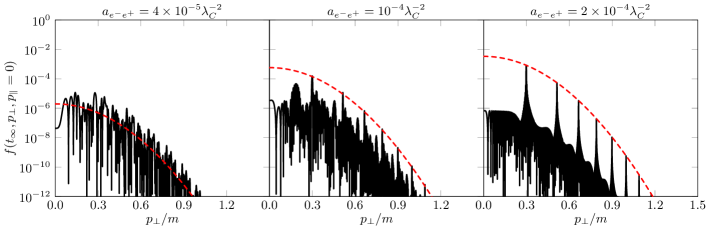
Figure 1: Residual phase space distribution $f(p_{\parallel}=0)$ as a function of transverse momentum $p_{\perp}$ for various pulse shapes (left panel: Gauss; middle panel: super-Gauss; right panel: flat-top). Parameters are $E_{1}=0.2E_{c}$, $\nu=0.02m$ and $n=1$, $\nu t_{G}=25\cdot 2\pi$ (left panel), $n=5$, $\nu t_{G}=25\cdot 2\pi$ (middle panel), $\nu t_{\text{ramp}}=5\cdot 2\pi$, $\nu t_{\text{flat}}=50\cdot 2\pi$ (right panel). As estimator of the density we use here $a_{e^{-}e^{+}}=2\pi\int\!\mathrm{d}p_{\perp}p_{\perp}f(p_{\perp},p_{\parallel}=0)$ depicted on top of the panels; the quantity $\lambda_{C}=\frac{h}{mc}$ is the Compton wavelength.

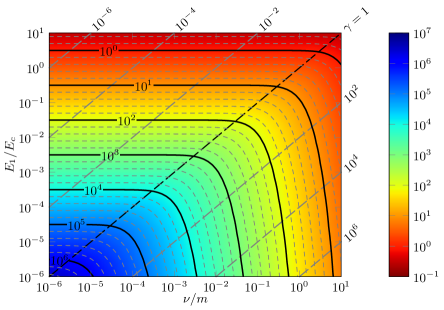
Figure 2: Contour plot of $4\frac{m}{\nu}G$, i.e. the negative of the exponent of $\mathcal{E}(\vec{p}=0)$ from Eq. (8), over the $E_{1}/E_{c}$ vs. $\nu/m$ plane. The solid black curves are contour lines at integer powers of $10$, the grey short dashed curves at $10^{0.2},\cdots,10^{0.8}$ between them. The long dashed lines are the loci of constant Keldysh parameter $\gamma=\gamma_{1}$.

$$\mathcal{J}=\begin{cases}t_{G}^{4/3},&\text{Gauss ($n=1$),}\\ t_{G}^{20/11},&\text{super-Gauss ($n=5$),}\\ t_{\text{flat}}^{2},&\text{flat-top pulse ($n\to\infty$).}\end{cases}$$ (11)

Figure 1 exhibits three examples for the transverse momentum spectrum at $p_{\parallel}=0$ for $N=1$, $E_{1}=0.2E_{c}$, $\nu=0.02m$ for a Gauss pulse (left panel, $n=1$, $\nu t_{G}=25\cdot 2\pi$) and a super-Gauss (middle panel, $n=5$, $\nu t_{G}=25\cdot 2\pi$) and a flat-top pulse (right panel, $\nu t_{\text{flat}}=50\cdot 2\pi$, $\nu t_{\text{ramp}}=5\cdot 2\pi$). In fact, (6’) delivers quite reliable estimates of the envelopes of the spectra. The latter ones require solutions of the quantum kinetic equations (1) for each value of $\vec{p}$ separately and with harsh numerical accuracy requirements. Thus, (6) and (6’) qualify for useful estimates of the maxima of the spectral distributions for several relevant pulse shapes, e.g. by considering $\mathcal{W}(p_{\perp}=0)$ as an estimator of the maximum peak height, supposed the pulse is flat enough. Obviously, the Gauss pulse is not flat enough; as a consequence, (6) and (6’) meet only the order of magnitude, at best.

To get a feeling for the parameter dependence of that maximum peak height, one can inspect the pulse-shape independent quantity $\mathcal{E}(p_{\perp}=0)$. Figure 2 exhibits the function $4\frac{m}{\nu}G(p_{\perp}=0,N=1)$ as a contour plot over the $E_{1}/E_{c}$ vs. $\nu/m$ plane. Since $\mathcal{E}=\exp\{-4\frac{m}{\nu}G\}$, large values of $4\frac{m}{\nu}G$ signal a strong suppression of the pair production. The region left/above the Keldysh line $\gamma_{1}=1$ (heavy dashed line) is the tunneling regime, where our above examples are located, while the region right/below the Keldysh line $\gamma_{1}=1$ belongs to the multi-photon regime.

3 Assisted Schwinger pair production

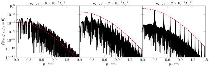
Figure 3: As in Fig. 1 but for the superposition of a second field with parameters $E_{2}=0.05E_{c}$, $N_{2}=25$.

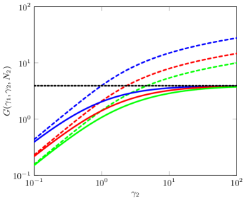
Figure 4: Plot of the function $G$ as defined in Eq. (8) as a function of $\gamma_{2}$ for $\nu=0.02m$, $\gamma_{1}=0.1$ and $N_{2}=9$ (blue), $N_{2}=17$ (red), $N_{2}=25$ (green). The horizontal black dotted curve is for the field 1 alone, therefore independent of $\gamma_{2}$. The dashed curves are for field 2 alone, and the solid curves for the superposition of both fields. Note that the residual pair density is proportional to $\exp\{-4\frac{m}{\nu}G\}$.

Superimposing to field 1 a second field 2, i.e. $N=2$ in (4), where the Keldysh parameter $\gamma_{2}$ refers to the multi-photon regime, can cause a significant enhancement of the pair production, as pioneered in schutzhold_dynamically_2008 (6, 7) and further exemplified in otto_lifting_2015 (21, 26). Figure 3 exhibits examples for $E_{1}=0.2E_{c}$, $\nu=0.02m$ (as in section 2) and $E_{2}=0.05E_{c}$, $N_{2}=25$ for pulse shape parameters as in Fig. 1. Also in the present case, the estimates (6) and (6’) are quite useful, in particular for the super-Gauss (middle panel) and flat-top pulse (right panel), while for the Gauss pulse (left panel) we meet again some underestimate. Quite indicative for the enhancement is the transversally integrated density, $a_{e^{-}e^{+}}=2\pi\int\!\mathrm{d}p_{\perp}p_{\perp}f(p_{\perp},p_{\parallel}=0)$ depicted at the top of the panels, which is in all displayed cases two orders of magnitude larger than the field 1 alone, as evident by comparison with the analog quantities in Fig. 1.

In the spirit of Fig. 2, one can inspect, for a rough orientation, the pulse shape independent function $\mathcal{E}$ or its heart, the function $G$, see Fig. 4. The dotted horizontal line is for field 1 alone, while the dashed curves depict field 2 alone, i.e. for $E_{1}=0$. Solid curves are for the fields 1+2. In fact, the solid curves, at fixed values of $E_{1,2}$ and $N_{2}$ are below the dotted and dashed ones pointing to lowering $G$ and thus to “lowering the exponential suppression”. As already observed in orthaber_momentum_2011 (29), there is a certain window where that enhancement is significant.

4 Doubly assisted Schwinger pair production

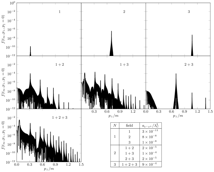
Figure 5: Residual transverse momentum spectra at $p_{\parallel}=0$ for three different fields and their combinations as indicated. The shape function used is the flat-top pulse. Parameters: $E_{1}=0.1E_{c}$, $\nu=0.07m$, $E_{2}=0.05E_{c}$, $N_{2}=7$, $E_{3}=0.01E_{c}$, $N_{3}=14$, $\nu t_{\text{ramp}}=5\cdot 2\pi$, $\nu t_{\text{flat}}=50\cdot 2\pi$. The table lists the transversally integrated spectra normalized to the square of the Compton wavelength.

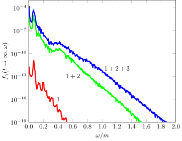
Figure 6: Final state spectra of photons emitted with frequency $\omega$ perpendicularly to the electric field (3) by the creation and subsequent motion of the $e^{+}$$e^{-}$ pairs. Field parameters and field nomenclature are as in the left column of Fig. (5).

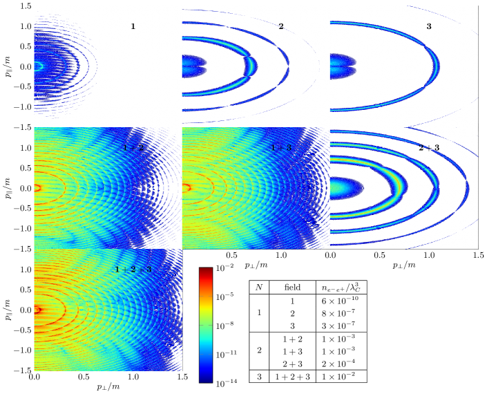
Figure 7: Color contour plots for the residual phase space distributions as in Fig. 5. The table lists the scaled densities.

It has been suggested in ilderton_nonperturbative_2015 (30) that adding shorter and shorter time-like inhomogeneities to the spatially homogeneous field causes further enhancement of the pair production. A realization of such a scenario is provided in torgrimsson_doubly_2016 (31) as doubly assisted pair production. We take the flat-top pulse shape and select $N=3$ with $E_{1}>E_{2}>E_{3}$ and $N_{1}=1<N_{2}<N_{3}$ such that $\gamma_{1}$ is in the tunneling regime and $\gamma_{2,3}$ in the multi-photon regime. Figure 5 exhibits the residual transverse momentum spectra for the three fields alone (top row), the pairwise combination of two fields (middle row) and the combination of all three fields (bottom left). The table (bottom right) lists the transversally integrated spectra. For the given parameters (see figure caption), the double assistance clearly causes an enhancement over the single assistance case. A similar enhancement is found in otto_afterglow_2017 (32) for the photons accompanying the $e^{+}e^{-}$ pair creation as a secondary probe. Figure 6 exhibits an example for the above field 1 alone (curve labelled by “1”), for the single assistance by field 2 (curve “1+2”), and the double assistance (curve “1+2+3”) as well. The fields “1”, “2” and “3” are the same as in Fig. 5. The calculations follow the first-order treatment of the quantized radiation field coupled to the $e^{+}$$e^{-}$ pairs as presented in otto_afterglow_2017 (32). One observes a huge assistance of the spectral photon yield $f_{\gamma}$ by the single field, while the double assistance causes only a mild further enhancement.

Figure 7 returns to $e^{+}$$e^{-}$ production and exhibits the momentum spectra as color contour plots and lists the normalized pair densities obtained by full momentum space integration. The latter values demonstrate the huge enhancement by multi-scale field configurations with a clear momentum signature.

5 Summary

Many previous studies show that the pulse shape of spatially homogeneous, oscillating electric fields has a decisive impact on the residual momentum distribution of the pairs emerging from the vacuum decay. We provide here some approximate formula which characterizes relevant features of the spectrum. In particular, such pulse shapes as super-Gauss or shape functions with a clear flat-top interval are proven to be uncovered by our formula. We supply, besides that generic consideration, some case studies for assisted and doubly assisted Schwinger pair creation. These can be considered as particular realisations of multi-scale pulses. Quite significant enhancement effects are found, also for the accompanying photons. While encouraging, we stress that spatial inhomogeneities counter act the enhancement. One has to go beyond the presently employed framework of the quantum kinetic equations to account properly for realistic field configurations.

Acknowledgements: The authors gratefully acknowledge inspiring discussions with H. Gies, R. Schützhold, R. Alkofer, D. B. Blaschke and C. Greiner. Many thanks go to S. Smolyansky and A. Panferov for common work on the plain Schwinger process. The fruitful collaboration with R. Sauerbrey and T. E. Cowan within the HIBEF project promoted the present investigation.

The interest of one of the authors (BK) in the present topic was initiated in a seminal physics colloquium at the TU Dresden in 1986 by Walter Greiner, where he surveyed the status and necessary future investigations towards understanding the quantum vacuum. We therefore dedicate our work to his legacy and acknowledge the collaborative work with colleagues and friends of Walter Greiner.

References

- (1) J. Schwinger “On Gauge Invariance and Vacuum Polarization” In Phys. Rev. 82, 1951, pp. 664
- (2) F. Gelis and N. Tanji “Schwinger mechanism revisited” In Prog. Part. Nucl. Phys. 87, 2016, pp. 1–49
- (3) F. Sauter “Über das Verhalten eines Elektrons im homogenen elektrischen Feld nach der relativistischen Theorie Diracs” In Z. Phys. 69.11 Springer-Verlag, 1931, pp. 742
- (4) E. Brezin and C. Itzykson “Pair Production in Vacuum by an Alternating Field” In Phys. Rev. D 2.7, 1970, pp. 1191–1199 DOI: 10.1103/PhysRevD.2.1191
- (5) N. B. Narozhny, S. S. Bulanov, V. D. Mur and V. S. Popov “-pair production by a focused laser pulse in vacuum” In Phys. Lett. A 330.1-2, 2004, pp. 1–6 DOI: 10.1016/j.physleta.2004.07.013
- (6) R. Schützhold, H. Gies and G. Dunne “Dynamically Assisted Schwinger Mechanism” In Phys. Rev. Lett. 101.13, 2008, pp. 130404 DOI: 10.1103/PhysRevLett.101.130404
- (7) G. V. Dunne, H. Gies and R. Schützhold “Catalysis of Schwinger vacuum pair production” In Phys. Rev. D 80.11, 2009, pp. 111301 DOI: 10.1103/PhysRevD.80.111301
- (8) I. Akal and G. Moortgat-Pick “Euclidean mirrors: enhanced vacuum decay from reflected instantons” In arXiv:1706.06447, 2017 arXiv:1706.06447 [hep-th]
- (9) H. Gies and G. Torgrimsson “Critical Schwinger Pair Production” In Phys. Rev. Lett. 116, 2016, pp. 090406
- (10) H. Gies and G. Torgrimsson “Critical Schwinger pair production. II. Universality in the deeply critical regime” In Phys. Rev. D 95, 2017, pp. 016001
- (11) J. Rafelski, B. Müller and W. Greiner “Spontaneous vacuum decay of supercritical nuclear composites” In Z. Phys. A Hadron. Nucl. 285.1, 1978, pp. 49
- (12) J. Rafelski, L. P. Fulcher and W. Greiner “Superheavy elements and an upper limit to the electric field strength” In Phys. Rev. Lett. 27, 1971, pp. 958–961 DOI: 10.1103/PhysRevLett.27.958
- (13) B. Müller, H. Peitz, J. Rafelski and W. Greiner “Solution of the Dirac equation for strong external fields” In Phys. Rev. Lett. 28, 1972, pp. 1235 DOI: 10.1103/PhysRevLett.28.1235
- (14) B. Müller, J. Rafelski and W. Greiner “Solution of the Dirac equation with two Coulomb centers” In Phys. Lett. B 47, 1973, pp. 5–7 DOI: 10.1016/0370-2693(73)90554-6
- (15) F. Fillion-Gourdeau, E. Lorin and A. D. Bandrauk “Enhanced Schwinger pair production in many-centre systems” In J. Phys. B 46.17, 2013, pp. 175002 URL: http://stacks.iop.org/0953-4075/46/i=17/a=175002
- (16) S. Augustin and C. Müller “Nonlinear Bethe-Heitler Pair Creation in an Intense Two-Mode Laser Field” In J. Phys.: Conf. Ser. 497.1, 2014, pp. 012020 DOI: 10.1088/1742-6596/497/1/012020
- (17) A. Di Piazza, E. Lötstedt, A. I. Milstein and C. H. Keitel “Effect of a strong laser field on electron-positron photoproduction by relativistic nuclei” In Phys. Rev. A 81.6, 2010
- (18) A. Di Piazza, C. Müller, K. Z. Hatsagortsyan and C. H. Keitel “Extremely high-intensity laser interactions with fundamental quantum systems” In Rev. Mod. Phys. 84.3, 2012, pp. 1177–1228
- (19) S. M. Schmidt, D. B. Blaschke, G. Röpke, S. A. Smolyansky, A. V. Prozorkevich and V. D. Toneev “A Quantum kinetic equation for particle production in the Schwinger mechanism” In Int. J. Mod. Phys. E 7, 1998, pp. 709 URL: http://arxiv.org/abs/hep-ph/9809227
- (20) S. Schmidt, D. B. Blaschke, G. Röpke, A. V. Prozorkevich, S. A. Smolyansky and V. D. Toneev “Non-Markovian effects in strong-field pair creation” In Phys. Rev. D 59.9, 1999, pp. 094005 URL: http://prd.aps.org/abstract/PRD/v59/i9/e094005
- (21) A. Otto, D. Seipt, D. Blaschke, B. Kämpfer and S. A. Smolyansky “Lifting shell structures in the dynamically assisted Schwinger effect in periodic fields” In Phys. Lett. B 740, 2015, pp. 335–340
- (22) C. Kohlfürst, M. Mitter, G. Winckel, F. Hebenstreit and R. Alkofer “Optimizing the pulse shape for Schwinger pair production” In Phys. Rev. D 88.4, 2013, pp. 045028 DOI: 10.1103/PhysRevD.88.045028
- (23) M. F. Linder, C. Schneider, J. Sicking, N. Szpak and R. Schützhold “Pulse shape dependence in the dynamically assisted Sauter-Schwinger effect” In Phys. Rev. D 92, 2015, pp. 085009
- (24) I. A. Aleksandrov, G. Plunien and V. M. Shabaev “Pulse shape effects on the electron-positron pair production in strong laser fields” In Phys. Rev. D 95, 2017, pp. 056013
- (25) Greger Torgrimsson, Christian Schneider, Johannes Oertel and Ralf Schützhold “Dynamically assisted Sauter-Schwinger effect — non-perturbative versus perturbative aspects” In J. High Energy Phys. 06, 2017, pp. 043
- (26) A. Otto, D. Seipt, D. B. Blaschke, S. A. Smolyansky and B. Kämpfer “Dynamical Schwinger process in a bifrequent electric field of finite duration: Survey on amplification” In Phys. Rev. D 91.10, 2015, pp. 105018 DOI: 10.1103/PhysRevD.91.105018
- (27) C. K. Dumlu and G. V. Dunne “Interference effects in Schwinger vacuum pair production for time-dependent laser pulses” In Phys. Rev. D 83.6, 2011, pp. 065028 DOI: 10.1103/PhysRevD.83.065028
- (28) H. Oppitz “Dynamisch assistierter Schwinger-Effekt für Multi-Skalen-Feldkonfigurationen”, 2017 URL: https://www.hzdr.de/db/Cms?pOid=55399
- (29) M. Orthaber, F. Hebenstreit and R. Alkofer “Momentum spectra for dynamically assisted Schwinger pair production” In Phys. Lett. B 698.1, 2011, pp. 80–85 DOI: 10.1016/j.physletb.2011.02.053
- (30) A. Ilderton, G. Torgrimsson and J. Wårdh “Nonperturbative pair production in interpolating fields” In Phys. Rev. D 92.6, 2015, pp. 065001
- (31) G. Torgrimsson, J. Oertel and R. Schützhold “Doubly assisted Sauter-Schwinger effect” In Phys. Rev. D 94, 2016, pp. 065035
- (32) A. Otto and B. Kämpfer “Afterglow of the dynamical Schwinger process: Soft photons amass” In Phys. Rev. D 95, 2017, pp. 125007