A gapped many-body system is described by a path integral on a space-time lattice $C^{d+1}$, which gives rise to a partition function $Z(C^{d+1})$ if $\partial C^{d+1}=\emptyset$, and a wave function $|\Psi\rangle$ on the boundary if $\partial C^{d+1}\neq\emptyset$. We show that $V=\text{log}\sqrt{\langle\Psi|\Psi\rangle}$ satisfies the inclusion-exclusion property $\frac{V(A\cup B)+V(A\cap B)}{V(A)+V(B)}=1$ and behaves like a volume of the space-time lattice $C^{d+1}$ in large lattice limit (i.e. thermodynamics limit). This leads to a proposal that the vector $|\Psi\rangle$ is the quantum-volume of the space-time lattice $C^{d+1}$. The quantum-volume satisfies a quantum additive property. The violation of the inclusion-exclusion property by $V=\text{log}\sqrt{\langle\Psi|\Psi\rangle}$ in the subleading term of thermodynamics limit gives rise to topological invariants that characterize the topological order in the system. This is a systematic way to construct and compute topological invariants from a generic path integral. For example, we show how to use non-universal partition functions $Z(C^{2+1})$ on several related space-time lattices $C^{2+1}$ to extract $(M_{f})_{11}$ and $\text{Tr}(M_{f})$, where $M_{f}$ is a representation of the modular group $SL(2,\mathbb{Z})$ – a topological invariant that almost fully characterizes the 2+1D topological orders.

Volume and Topological Invariants of Quantum Many-body Systems

Introduction: Recently, it was proposed that all force particles (the gauge bosons) and matter particles (the fermions) may arise from entangled quantum information if we assume the space to be an ocean of qubits Wen (2003); Levin and Wen (2006a); Wen (2013); You et al. (2014); You and Xu (2015). If the physical space is indeed an entangled ocean of qubits, then it is natural to suspect that the mathematical notion of continuous space (i.e. the notion of manifold) may also arise from entangled qubits that are discrete and algebraic in nature. This leads to a current very active research direction trying to view continuous geometry as emergent from discrete algebra. This point of view may lead to a quantum theory of gravity Maldacena (1998); Lee (2010) – a long-sought-after goal of fundamental theoretical physics. However, at the moment, we still do not know how the metrics of a manifold, and Einstein equation that govern the dynamics of metrics as the only low energy excitations, can emerge from discrete and entangled qubits. (For the emergence of non-Einstein quantum gravity as the only low energy dynamics, see LABEL:X0643,GW0600,GW1290.) In this paper, we will address a much simpler question: how the volume emerges from discrete and entangled qubits. We would like to demonstrate that at least one geometric quantity, the volume, can emerge from discrete algebra.

It turns out that if we only have emergent volume, the associated space does not have a sense of “shape” and its dynamics is not governed by Einstein’s theory of gravity, but by a different gravitational theory – a topological quantum field theory Witten (1989); Atiyah (1988). We may call this kind of gravity as topological gravity. There are many examples to demonstrate how various topological gravity (i.e. various topological quantum field theories) emerge from entangled qubits (i.e. entangled many-body systems). The emergence of topological quantum field theories from entangled many-body systems is well studied in condensed matter physics under the name of topological order Wen (1990); Wen and Niu (1990). Thus, entangled many-body systems can also give us topological gravity and a sense of volume – an emerging geometric property.

At the first sight, the issue of emergent volume appears to be trivial for many-body systems, since every many-body system has a natural definition of volume: the number of lattice sites. However, this only works for translation symmetric many-body system. For many-body systems without translation symmetry, it is not proper to define the volume as the number of lattice sites. Now we can state the main issue that we try to address in this paper: how to define the notion of volume for a non-translation symmetric many-body systems on lattice?

We find that if a quantum many-body system is in a topologically ordered phase (or more precisely, a gapped quantum liquid state), then the notion of volume can be defined even without translation symmetry. However, the volume that directly arise from the many-body system is not exactly the volume in the familiar classical sense. We will call the new notion of volume as quantum volume. Unlike classical volume which is a positive real number, a quantum volume is not a real number, but a vector in a Hilbert space.

From the quantum volume of a many-body system, we may define an emergent classical volume as the norm of the quantum volume (i.e. the norm of the vector). We find that such classical volume does not satisfy the classical volume axioms exactly. However, in the large system size limit (the thermodynamical limit), the leading term of the classical volume does satisfy the classical volume axioms.

We also find that the finite subleading terms that violate the classical volume axioms vanishes for many-body states with trivial topological order (i.e. for product states). So non-vanishing subleading terms imply a non-trivial topological order. In fact, those finite subleading terms are topological invariants that characterize the underlying topological order.

This is very similar to entanglement entropy: the leading term of entanglement entropy can be used to define the total area of the interface, while the finite subleading term – the topological entanglement entropy – is a topological invariant that characterize the underlying topological order Kitaev and Preskill (2006); Levin and Wen (2006b). We speculate that the two could be related by some generalization of the Fubini’s theorem.

Volume in quantum many-body system: To define a many-body system through a space-time path integral, we first triangulate the $d+1$-dimensional space-time to obtain a simplicial complex $C_{N}$ with $N$ vertices. The degrees of freedom of our lattice model live on the vertices (denoted by $v_{i}$ where $i$ labels the vertices), on the edges (denoted by $e_{ij}$ where $\langle ij\rangle$ labels the edges), etc . The action amplitude $\hskip 1.0pt\mathrm{e}^{S_{\text{cell}}}$ for an $n$-cell $(ij\cdots k)$ is complex function of $v_{i}$, $e_{ij},\cdots$ on the cell: $T_{ij\cdots k}(\{v_{i}\},\{e_{ij}\},\cdots)$. The total action amplitude $\hskip 1.0pt\mathrm{e}^{S}$ for a configuration $\{v_{i}\},\{e_{ij}\},\cdots$ (or a path) is given by

$$\hskip 1.0pt\mathrm{e}^{S}=\prod_{(ij\cdots k)}T_{ij\cdots k}(\{v_{i}\},\{e_{ij}\},\cdots)$$ (1)

where $\prod_{(ij\cdots k)}$ is the product over all the $n$-cells $(ij\cdots k)$. Our lattice theory is defined by the following imaginary-time path integral (or partition function)

$$Z(\{v^{\text{bdry}}_{i},e^{\text{bdry}}_{ij},\cdots\},C_{N}^{d+1},T)=\hskip-10.00002pt\sum_{\{v_{i}\},\{e_{ij}\},\cdots}\hskip-10.00002pt\hskip 1.0pt\mathrm{e}^{S}:=|\Psi(C_{N}^{d+1})\rangle$$ (2)

where $\sum_{\{v_{i}\},\{e_{ij}\},\cdots}$ only sum over the indices inside the space-time complex, and the indices $v^{\text{bdry}}_{i},e^{\text{bdry}}_{ij},\cdots$ on the boundary of the space-time complex are fixed. We see that on space-time with boundary, the path integral gives rise to a wave function on the boundary $|\Psi\rangle$. On space-time with no boundary, the path integral gives rise to a complex number – the partition function $Z(C_{N}^{d+1},T)$. (In the above dicussion, some important details are ignored. More precise description can be found in the supplementary material and in LABEL:KW1458.)

In the $N\to\infty$ thermodynamic limit, the partition function is roughly given by

$$\ \ \ \ Z(\{v^{\text{bdry}}_{i},e^{\text{bdry}}_{ij}\},C^{d+1}_{N},T)$$

$$=\hskip 1.0pt\mathrm{e}^{S^{\text{eff}}_{N}}Z^{\text{top}}(\{v^{\text{bdry}}_{i},e^{\text{bdry}}_{ij}\},C^{d+1}_{N},T),$$ (3)

where $S^{\text{eff}}_{N}=\int_{\text{space-time}}\text{energy-density}\propto N$, and $Z^{\text{top}}(\{v^{\text{bdry}}_{i},e^{\text{bdry}}_{ij}\},C^{d+1}_{N},T)$ is independent of $N$. (The notion of topological partition function $Z^{\text{top}}$ and topological path integral are discussed in more detail in the supplementary material and in LABEL:KW1458.) We see that the leading term $S^{\text{eff}}_{N}$ behaves like a volume. Thus we will call $V(C^{d+1}_{N},T)$ defined by

$$V(C^{d+1}_{N},T)=\log\sqrt{\langle\Psi|\Psi\rangle}$$ (4)

as the (classical) space-time volume. In other words, the many-body system described by the tensor $T$ and triangulation $C^{d+1}_{N}$ give raise to a definition of classical volume of the space-time. At the leading order of $N$, such a classical volume, $V(C^{d+1}_{N},T)=S^{\text{eff}}_{N}=\int_{\text{space-time}}\text{energy-density}$, satisfies the inclusion-exclusion property: Let $Y$ be a $d$-dimensional manifold with a Riemannian metric $\gamma$ and $\mathcal{M}_{(Y,\gamma)}$ the set of all Riemannian manifolds $(X,g)$ such that $\partial X=Y$ and $g|_{Y}=\gamma$. Then the volume functional $V:\mathcal{M}_{(Y,\gamma)}\rightarrow\mathbb{R}$ satisfies the inclusion-exclusion formula

$$V(A)+V(B)=V(A\cup B)+V(A\cap B),$$ (5)

We like to mention that the Euler characteristic $\chi(X)$ of a topological space $X$ usually appears in the path integrals as a prefactor $a^{\chi}$ (just like $\hskip 1.0pt\mathrm{e}^{S^{\text{eff}}_{N}}$) and behave like a volume. The Euler characteristic has an axiomatic characterization. The Euler characteristic $\chi(X)$ is essentially the only homotopy invariant function on all topological spaces that satisfies the multiplicative property $\chi(X\times Y)=\chi(X)\chi(Y)$ and the inclusion-exclusion formula $\chi(X)=\chi(A)+\chi(B)-\chi(A\cap B)$ if $X=A\cup B$. But there are no known axiomatic characterizations of the volume functional.

To discuss volume more precisely, i.e. to include both terms at the $N$-order and the $N^{0}$-order, it is better to introduce a notion of quantum volume, or q-volume. A q-volume is not a real number. It is a vector, i.e. the wave function $|\Psi\rangle$. The norm of the q-volume gives rise to the corresponding classical volume. We like to stress that the above definition of q-volume is very general. It applies to both gapped many-body systems and gapless many-body systems. In this paper, we will concentrate on gapped many-body systems.

A topological invariant that is closely related to volume is the Gromov norm of the fundamental class of a manifold. The Gromov norm behaves well with respect to covering maps, so one test for quantum volume would be to study its behavior under covering maps. Quantum volumes also satisfy some neutrality and gluing properties. For a many-body system described by tensor $T$, its q-volume satisfies

$$\ \ \ \ |\Psi(C^{d+1}_{1}\cup C^{d+1}_{2})\rangle$$

$$={\rm Tr}_{\partial C^{d+1}_{1}\cap\partial C^{d+1}_{2}}[|\Psi(C^{d+1}_{1})\rangle\otimes|\Psi(C^{d+1}_{2})\rangle]$$ (6)

if the space-time complexes $C^{d+1}_{1}$ and $C^{d+1}_{2}$ only overlap on their boundaries. Here ${\rm Tr}_{\partial C^{d+1}_{1}\cap\partial C^{d+1}_{2}}$ traces over the degrees of freedom on the overlapped boundaries $\partial C^{d+1}_{1}\cap\partial C^{d+1}_{2}$. Since $|\Psi\rangle$’s are exponentially large $\hskip 1.0pt\mathrm{e}^{S^{\text{eff}}_{N}}$ in large $N$ limit, from (Volume and Topological Invariants of Quantum Many-body Systems), we can show that, in thermodynamic limit, the corresponding classical volume satisfies

$$\frac{V(C^{d+1}_{1}\cup C^{d+1}_{2})}{V(C^{d+1}_{1})+V(C^{d+1}_{2})}=1$$ (7)

which is a special case of (5).

Topological invariant through q-volume and surgery: In general the partition function $Z(C^{d+1}_{N},T)=\hskip 1.0pt\mathrm{e}^{S^{\text{eff}}_{N}}Z^{\text{top}}$ of a many-body system is not a topological invariant even when the many-body system described by the tensor $T$ realizes a topologically ordered state. In the absence of translation symmetry, it is not trivial to separate the non-universal part $\hskip 1.0pt\mathrm{e}^{S^{\text{eff}}_{N}}$ from the topological invariant $Z^{\text{top}}$ by just knowing $Z(C^{d+1}_{N},T)$.

To achieve the separation, we note that, the $S^{\text{eff}}_{N}$ part of $\log|Z(C^{d+1}_{N},T)|$ is the standard classical volume of the space-time that satisfy the inclusion-exclusion property (5). Thus, we can separate the $Z^{\text{top}}$ part of the partition function, since $Z^{\text{top}}$ violates the properties of classical volume. $Z^{\text{top}}$ is the topological invariant that reflects the non-trivial topological order in the system. In other words, for a system with trivial topological order, the classical volume axioms are satisfied even at $\hskip 1.0pt\mathrm{e}^{N^{0}}$ order, i.e. $Z^{\text{top}}=1$ (see (9)).

As an application of the above idea, we consider the following ratio of two partition functions for a many-body system described by a tensor-set $T$:

$${Z\Big{(}\begin{matrix}\includegraphics[height=43.36243pt]{MNB}\end{matrix},T\Big{)}}\Big{/}{Z\Big{(}\begin{matrix}\includegraphics[height=43.36243pt]{MNB1}\end{matrix},T\Big{)}}$$ (8)

Here, we divide the $d+1$-dimensional space-time $M$ into two parts $M_{U}$ and $M_{D}$ by a $d$-dimensional boundary with a triangulation $B$. We also divide the other space-time $N$ into two parts $N_{U}$ and $N_{D}$ by a boundary with the same triangulation $B$. This allows us to glue $M_{U}$ with $N_{D}$ and $N_{U}$ with $M_{D}$.

If $V=\log|Z|$ exactly satisfy the inclusion-exclusion property of the classical volume, then the above ratio (8) will be 1. However, in general, the subleading $N^{0}$-term in $V=\log|Z|$ does not satisfy the inclusion-exclusion property. Such subleading terms will make the ratio (8) to differ from 1. But for a system $T$ with trivial topological order, we find that the above ratio (8) will be 1 in the thermodynamic limit. This is because the partition functions and their ratio is invariant under the tensor network renormalization transformations which coarse grain the tensor network away from the boundary $B$. If the tensor $T$ describes a trivial topological order, the tensor network will flow to a corner-double-line tensor network in 1+1D or a similar structured tensor network in higher dimensions Gu and Wen (2009):

$$\ \ \ \ {Z\Big{(}\begin{matrix}\includegraphics[height=43.36243pt]{MNBT}\end{matrix},T\Big{)}}\Big{/}{Z\Big{(}\begin{matrix}\includegraphics[height=43.36243pt]{MNB1T}\end{matrix},T\Big{)}}$$ (9)

$$={Z\Big{(}\begin{matrix}\includegraphics[height=43.36243pt]{MNBT1}\end{matrix},T\Big{)}}\Big{/}{Z\Big{(}\begin{matrix}\includegraphics[height=43.36243pt]{MNB1T1}\end{matrix},T\Big{)}}=1$$

This allows us to show the ratio (8) to be 1, if the system has no topological order. Thus the ratio (8) is a topological invariant that can characterize non-trivial topological orders in the system.

The following ratio is also a topological invariant

$${Z\Big{(}\begin{matrix}\includegraphics[scale={0.3}]{MUD}\end{matrix},T\Big{)}}\Big{/}\sqrt{Z\Big{(}\begin{matrix}\includegraphics[scale={0.25}]{MUU}\end{matrix},T\Big{)}Z\Big{(}\begin{matrix}\includegraphics[scale={0.25}]{MDD}\end{matrix},T\Big{)}}$$ (10)

The above ratio is calculated by dividing the closed space-time $M$ into two parts $M=M_{U}\cup M_{D}$. It not only dependent on the space-time $M$, it also depends on $M_{U}$ and $M_{D}$, i.e. how we partition $M$. Notice that the space-time with boundary, $M_{U}$ and $M_{D}$, give rise to two vectors $\langle\Psi(M_{U})|$ and $|\Psi(M_{D})\rangle$, which are not normalized. The above ratio is simply the overlap of $\langle\Psi(M_{U})|$ and $|\Psi(M_{D})\rangle$ after normalization: $\frac{\langle\Psi(M_{U})|\Psi(M_{D})\rangle}{\sqrt{\langle\Psi(M_{U})|\Psi(M_{U})\rangle}\sqrt{\langle\Psi(M_{D})|\Psi(M_{D})\rangle}}$.

Let us apply the above approaches to construct some topological invariants. First, for $d+1$D many-body systems with unique gapped liquid ground state on $S^{d}$,

$$\ \ \ \ {Z\Big{(}\begin{matrix}\includegraphics[height=43.36243pt]{MNB}\end{matrix},T\Big{)}}\Big{/}{Z\Big{(}\begin{matrix}\includegraphics[height=43.36243pt]{MNB1}\end{matrix},T\Big{)}}$$

$$=\frac{Z(M_{U}\cup M_{D})Z(N_{U}\cup N_{D})}{Z(N_{U}\cup M_{D})Z(M_{U}\cup N_{D})}=\Big{|}_{B=S^{d}}1$$ (11)

So when the partition boundary is a sphere $B=S^{d}$, the above ratio fails to give rise to any non-trivial topological invariant. Thus, the connected sum decomposition does not give rise to non-trivial topological invariants. The non-trivial topological invariants may arise when the division has a non-trivial cross section $B$ beyond a sphere.

One such topological invariant is obtained by choosing $M_{U}=D^{2}\times S^{1},\ M_{D}=D^{2}\times S^{1},\ N_{U}=S^{1}\times D^{2},\ N_{D}=S^{1}\times D^{2}$. We find

$$\ \ \ \ \frac{Z(D^{2}\times S^{1}\cup D^{2}\times S^{1})Z(S^{1}\times D^{2}\cup S^{1}\times D^{2})}{Z(S^{1}\times D^{2}\cup D^{2}\times S^{1})Z(D^{2}\times S^{1}\cup S^{1}\times D^{2})}$$

$$=\Big{|}_{N\to\infty}\Big{(}\frac{Z^{\text{top}}(S^{2}\times S^{1})}{Z^{\text{top}}(S^{3})}\Big{)}^{2}=D^{2}$$ (12)

which allows us to calculate the total quantum dimension $D^{2}=\sum d_{i}^{2}$ of a 2+1D topologically ordered state. Here, $D^{2}\times S^{1}\cup D^{2}\times S^{1}=S^{2}\times S^{1}$ is obtained by glueing two solid tori $D^{2}\times S^{1}$, and $S^{1}\times D^{2}\cup D^{2}\times S^{1}=S^{3}$ is obtained by glueing two solid tori in a twisted way.

Also $N\to\infty$ is the limit of more and more refined triangulation of the space-time (i.e. the thermodynamics limit in condensed matter physics). To obtain the first equal sign in (Volume and Topological Invariants of Quantum Many-body Systems) we have used the fact that the leading term $S^{\text{eff}}_{N}$ in the partition function satisfies the inclusion-exclusion property of the classical volume in $N\to\infty$ limit. This is because the leading $S^{\text{eff}}_{N}$ is given by the integration of local energy density over space-time. We can always tune the local energy density continuously without encounter any phase transition. Thus we can tune $S^{\text{eff}}_{N}$ to zero without any phase transition. This leads to the first equal sign in (Volume and Topological Invariants of Quantum Many-body Systems).

Another topological invariant is given by

$$\ \ \ \ \frac{Z(D^{2}\times S^{1}\times S^{1}\cup D^{2}\times S^{1}\times S^{1})Z(S^{1}\times D^{2}\times S^{1}\cup S^{1}\times D^{2}\times S^{1})}{Z(S^{1}\times D^{2}\times S^{1}\cup D^{2}\times S^{1}\times S^{1})Z(D^{2}\times S^{1}\times S^{1}\cup S^{1}\times D^{2}\times S^{1})}=\Big{|}_{N\to\infty}\Big{(}\frac{Z^{\text{top}}(S^{2}\times S^{1}\times S^{1})}{Z^{\text{top}}(S^{3}\times S^{1})}\Big{)}^{2}=N_{p}^{2}$$ (13)

which allows us to calculate the number $N_{p}$ of topological types of point-like excitations of a 3+1D topologically ordered state.

We can also use (10) to construct more topological invariants. First, let $M_{U}$ and $M_{D}$ be handlebodies of genus $g$, and let $f$ be an orientation reversing homeomorphism from the boundary of $B=\partial M_{U}$ to the boundary of $B=\partial M_{D}$. By gluing $M_{U}$ to $M_{D}$ along $B$ we obtain the compact oriented 3-manifold $M=V\cup_{f}W$. Every closed, orientable three-manifold may be so obtained, which is called a Heegaard splitting. Thus we can construct a topological invariant for each orientable three-manifold and its Heegaard splitting.

More specifically, we can choose $M_{U}=D^{2}\times S^{1}$, $M_{D}=D^{2}\times S^{1}$, and $f$ be a mapping from $S^{1}\times S^{1}$ to $S^{1}\times S^{1}$. Thus $f$ is an element in $SL(2,\mathbb{Z})$. In this case we find that

$${Z\Big{(}\begin{matrix}\includegraphics[scale={0.3}]{MUD}\end{matrix},T\Big{)}}\Big{/}\sqrt{Z\Big{(}\begin{matrix}\includegraphics[scale={0.25}]{MUU}\end{matrix},T\Big{)}Z\Big{(}\begin{matrix}\includegraphics[scale={0.25}]{MDD}\end{matrix},T\Big{)}}=\Big{|}_{N\to\infty}$$

$${Z^{\text{top}}\Big{(}\begin{matrix}\includegraphics[scale={0.3}]{MUD}\end{matrix},T\Big{)}}\Big{/}\sqrt{Z^{\text{top}}\Big{(}\begin{matrix}\includegraphics[scale={0.25}]{MUU}\end{matrix},T\Big{)}Z^{\text{top}}\Big{(}\begin{matrix}\includegraphics[scale={0.25}]{MDD}\end{matrix},T\Big{)}}$$

$$=(M_{f})_{11},$$ (14)

where $M_{f}$ is the representation of $SL(2,\mathbb{Z})$ in the quasiparticle basis Wen (1990); Keski-Vakkuri and Wen (1993); Zhang et al. (2012).

We may also choose $M_{U}=I^{1}\times T^{2}\cup_{f}I^{1}\times T^{2}$, and $M_{D}=I^{1}\times T^{2}$. Note that $I^{1}\times T^{2}$ has two $T^{2}=S^{1}\times S^{1}$ boundaries. $M_{U}$ is formed by two $I^{1}\times T^{2}$’s glued along one of the $T^{2}$ boundary with a $f$-twist. Then, we glue the two $T^{2}$ boundaries of $M_{U}$ and two $T^{2}$ boundaries of $M_{D}$ directly without twist to form the total space-time lattice. In this case we find that

$${Z\Big{(}\begin{matrix}\includegraphics[scale={0.3}]{MUD}\end{matrix},T\Big{)}}\Big{/}\sqrt{Z\Big{(}\begin{matrix}\includegraphics[scale={0.25}]{MUU}\end{matrix},T\Big{)}Z\Big{(}\begin{matrix}\includegraphics[scale={0.25}]{MDD}\end{matrix},T\Big{)}}=\Big{|}_{N\to\infty}$$

$${Z^{\text{top}}\Big{(}\begin{matrix}\includegraphics[scale={0.3}]{MUD}\end{matrix},T\Big{)}}\Big{/}\sqrt{Z^{\text{top}}\Big{(}\begin{matrix}\includegraphics[scale={0.25}]{MUU}\end{matrix},T\Big{)}Z^{\text{top}}\Big{(}\begin{matrix}\includegraphics[scale={0.25}]{MDD}\end{matrix},T\Big{)}}$$

$$={\rm Tr}(M_{f})/\text{dim}{M_{f}}.$$ (15)

$M_{f}$ is an important topological invariant that characterizes the topological order in the many-body system.

The above expression allows us to compute the topological invariants $(M_{f})_{11}$ and ${\rm Tr}(M_{f})$ using generic non-fixed point path integral $Z\Big{(}\begin{matrix}\includegraphics[scale={0.2}]{MUD}\end{matrix},T\Big{)}$ in the thermodynamical limit. We like to stress that in (Volume and Topological Invariants of Quantum Many-body Systems), we need to choose the triangulation on $M_{U}=D^{2}\times S^{1}$ and $M_{D}=D^{2}\times S^{1}$, such that the induced triangulation on the common boundary $B=\partial D^{2}\times S^{1}$ is related by the mapping $f$.

We know that $SL(2,\mathbb{Z})$ is generated by $S$ for $f=\begin{pmatrix}0&-1\\ 1&0\\ \end{pmatrix}$ and $T$ for $f=\begin{pmatrix}1&1\\ 0&1\\ \end{pmatrix}$. By choosing different $f$’s, we can obtain $S_{11}$, $T_{11}$, $(ST)_{11}$, etc in the quasiparticles basis.

Summary: We introduce a notion of quantum volume for quantum many-body systems defined on space-time lattice. The quantum volume is not a positive number but a vector in a Hilbert space, which satisfies an additive property (Volume and Topological Invariants of Quantum Many-body Systems). We show that the norm of the quantum volume gives rise to classical volume that satisfies the inclusion-exclusion property (5) in the thermodynamic limit.

For a many-body system with topological order, its partition function is not universal and depends in the details of interaction. Using the idea of quantum volume and classical volume, we show how to compute topological invariants from non-universal partition functions. In particular, we show how to compute the trace and the $(1,1)$ matrix element of the modular representation in quasiparticle basis from non-universal 2+1D partition functions.

X.-G Wen is partially supported by NSF grant DMR-1506475, DMS-1664412, and NSFC 11274192. Z. Wang is partially funded by NSF grant DMS-1411212 and FRG-1664351.

Supplementary Materials

Appendix A Many-body systems and path integral on space-time lattice

In this section, we will define many-body systems without translation symmetry via space-time path integral. We will define space-time path integral using uniform tensors on arbitrary random space-time lattice. Despite the tensors are uniform, the random space-time lattice breaks the translation symmetry. Later we will use such space-time path integral to define the quantum and classical volumes of the random space-time lattice.

A.1 Space-time complex

To define a Many-body system through a space-time path integral, we first triangulate the $n$-dimensional space-time to obtain a simplicial complex $C_{N}$ (see Fig. 1). Here we assume that all simplicial complexes are of bounded geometry in the sense that the number of edges that connect to one vertex is bounded by a fixed value. Also the number of triangles that connect to one edge is bounded by a fixed value, etc .

In order to define a generic lattice theory on the space-time complex $C_{N}$, it is important to give the vertices of each simplex a local order. A nice local scheme to order the vertices is given by a branching structure.Costantino (2005); Chen et al. (2013, 2012) A branching structure is a choice of orientation of each edge in the $n$-dimensional complex so that there is no oriented loop on any triangle (see Fig. 2).

The branching structure induces a local order of the vertices on each simplex. The first vertex of a simplex is the vertex with no incoming edges, and the second vertex is the vertex with only one incoming edge, etc . So the simplex in Fig. 2a has the following vertex ordering: $0<1<2<3$.

The branching structure also gives the simplex (and its sub simplexes) an orientation denoted by $s_{ij\cdots k}=1,*$. Fig. 2 illustrates two $3$-simplices with opposite orientations $s_{0123}=1$ and $s_{0123}=*$. The red arrows indicate the orientations of the $2$-simplices which are the subsimplices of the $3$-simplices. The black arrows on the edges indicate the orientations of the $1$-simplices.

A.2 Path integral on a space-time complex

Figure 1: A 2-dimensional complex. The vertices (0-simplices) are labeled by $i$. The edges (1-simplices) are labeled by $\langle ij\rangle$. The faces (2-simplices) are labeled by $\langle ijk\rangle$. The degrees of freedoms may live on the vertices (labeled by $v_{i}$), on the edges (labeled by $e_{ij}$) and on the faces (labeled by $\phi_{ijk}$).

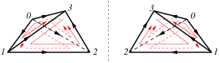
Figure 2: (Color online) Two branched simplices with opposite orientations. (a) A branched simplex with positive orientation and (b) a branched simplex with negative orientation.

The degrees of freedom of our lattice model live on the vertices (denoted by $v_{i}$ where $i$ labels the vertices), on the edges (denoted by $e_{ij}$ where $\langle ij\rangle$ labels the edges), and on other high dimensional simplicies of the space-time complex (see Fig. 1). The action amplitude $\hskip 1.0pt\mathrm{e}^{S_{\text{cell}}}$ for an $n$-cell $(ij\cdots k)$ is complex function of $v_{i}$, $e_{ij},\cdots$: $T_{ij\cdots k}(\{v_{i}\},\{e_{ij}\},\cdots)$. The total action amplitude $\hskip 1.0pt\mathrm{e}^{S}$ for a configuration $\{v_{i}\},\{e_{ij}\},\cdots$ (or a path) is given by

$$\hskip 1.0pt\mathrm{e}^{S}=\prod_{(ij\cdots k)}[T_{ij\cdots k}(\{v_{i}\},\{e_{ij}\},\cdots)]^{s_{ij\cdots k}}$$ (16)

where $\prod_{(ij\cdots k)}$ is the product over all the $n$-cells $(ij\cdots k)$. Note that the contribution from an $n$-cell $(ij\cdots k)$ is $T_{ij\cdots k}(\{v_{i}\},\{e_{ij}\},\cdots)$ or $T^{*}_{ij\cdots k}(\{v_{i}\},\{e_{ij}\},\cdots)$ depending on the orientation $s_{ij\cdots k}$ of the cell. Our lattice theory is defined by the following imaginary-time path integral (or partition function)

$$Z=\sum_{\{v_{i}\},\{e_{ij}\},\cdots}\prod_{(ij\cdots k)}[T_{ij\cdots k}(\{v_{i}\},\{e_{ij}\},\cdots)]^{s_{ij\cdots k}}.$$ (17)

Clearly, the partition function $Z$ depends on the space-time $M$, so we denote it as $Z(M)$. It is also clear that the partition function on a disjoint union of $M$ and $N$ is given by the product of the two partition functions on $M$ and on $N$:

$$Z(M\sqcup N)=Z(M)Z(N)$$ (18)

We would like to point out that, in general, the path integral may also depend on some additional weighting factors $w_{v_{i}}$, ${d}_{e_{ij}}^{v_{i}v_{j}}$, etc (see (23)). In this section, for simplicity, we will assume those weighting factors are all equal to $1$.

In the above path integral (17), we have assigned the same action amplitude $T_{ij\cdots k}(\{v_{i}\},\{e_{ij}\},\cdots)$ to each simplex $(ij\cdots k)$. Such a path integral is called a uniform path integral. For simplicity, in this paper, we only study systems described by uniform path integral. But our discussion also apply the more complicated cases where different simplices $(ij\cdots k)$ have different action amplitudes.

Figure 3: Each time-step of evolution is given by the path integral on a particular form of branched graph. Here is an example in 1+1D.

Figure 4: The reduction of double-layer time-step to single-layer time-step on space with boundary for an 1+1D topological path integral.

A.3 Path integral on a space-time complex with boundary

In the last subsection, we have defined the path integral on a space-time complex without boundary. In this case, all the indices on vertices, edges, etc are summed over. The resulting partition function $Z$ is just a complex number.

If the space-time manifold has a boundary $\partial M^{d+1}=M_{B}^{d}$, then the triangulation $C^{d+1}_{N}$ of $M^{d+1}$ has the following property: all the vertices in $C^{d+1}_{N}$ that are on the boundary $M_{B}^{d}$ form a subcomplex $B^{d}_{N^{\prime}}$, such that $B^{d}_{N^{\prime}}$ is a triangulation of $M_{B}^{d}$. In this case, we say that the complex $C^{d+1}_{N}$ has a boundary which is given by $B^{d}_{N^{\prime}}\equiv\partial C^{d+1}_{N}$.

The path integral on $C^{d+1}_{N}$ with a boundary is defined differently: we only sum over the indices on vertices, edges, etc that are not on the boundary $B^{d}_{N^{\prime}}$. The indices on the boundary $B^{d}_{N^{\prime}}$ are fixed. So the resulting partition function $Z$ is a function of the indices on the boundary $B^{d}_{N^{\prime}}$. We see that the boundary $B^{d}_{N^{\prime}}$ gives rise to a Hilbert space ${\cal H}_{B^{d}_{N^{\prime}}}$ formed by all the complex functions of the indices on the boundary $B^{d}_{N^{\prime}}$. The partition function $Z$ on $C^{d+1}_{N}$ is a vector in ${\cal H}_{B^{d}_{N^{\prime}}}$ (i.e. a particular complex function of the indices on $B^{d}_{N^{\prime}}$). This is consistent with the Atiyah’s definition of topological quantum field theory Atiyah (1988).

A.4 Path integral and Hamiltonian

Consider a space-time complex of topology $M_{\text{space}}\times I$ where $I=[t,t^{\prime}]$ represents the time dimension and $M_{\text{space}}$ is a closed space complex (see Fig. 3). The space-time complex $M_{\text{space}}\times I$ has two boundaries: one at time $t$ and another at time $t^{\prime}$. A path integral on the space-time complex $M_{\text{space}}\times I$ is a function of the indices on the two boundaries, which give us an amplitude $Z[\{v_{i}^{\prime},e_{ij}^{\prime},\cdots\},\{v_{i},e_{ij},\cdots\}]$ from a configuration $\{v_{i},e_{ij},\cdots\}$ at $t$ to another configuration $\{v_{i}^{\prime},e_{ij}^{\prime},\cdots\}$ at $t^{\prime}$. Here, $\{v_{i},e_{ij},\cdots\}$ and $\{v_{i}^{\prime},e_{ij}^{\prime},\cdots\}$ are the degrees of freedom on the boundaries (see Fig. 3). We like to interpret $Z[\{v_{i}^{\prime},e_{ij}^{\prime},\cdots\},\{v_{i},e_{ij},\cdots\}]$ as the amplitude of an evolution in imaginary time by a Hamiltonian:

$$\ \ \ \ Z[\{v_{i}^{\prime},e_{ij}^{\prime},\cdots\},\{v_{i},e_{ij},\cdots\}]$$

$$=\langle v_{i}^{\prime},e_{ij}^{\prime},\cdots|\hskip 1.0pt\mathrm{e}^{-(t^{\prime}-t)H}|v_{i},e_{ij},\cdots\rangle.$$ (19)

However, such an interpretation may not be valid since $Z[\{v_{i}^{\prime},e_{ij}^{\prime},\cdots\},\{v_{i},e_{ij},\cdots\}]$ may not give raise to a Hermitian matrix. It is a worrisome realization that path integral and Hamiltonian evolution may not be directly related.

Here we would like to use the fact that the path integral that we are considering are defined on the branched graphs with a “reflection” property (see (16)). We like to show that such path integral are better related Hamiltonian evolution. The key is to require that each time-step of evolution is given by branched graphs of the form in Fig. 3. One can show that $Z[\{v_{i}^{\prime},e_{ij}^{\prime},\cdots\},\{v_{i},e_{ij},\cdots\}]$ obtained by summing over all in the internal indices in the branched graphs Fig. 3 has a form

$$\ \ \ \ Z[\{v_{i}^{\prime},e_{ij}^{\prime},\cdots\},\{v_{i},e_{ij},\cdots\}]$$ (20)

$$=\sum_{\{v_{i}^{\prime\prime},e_{ij}^{\prime\prime},\cdots\}}U^{*}[\{v_{i}^{\prime\prime},e_{ij}^{\prime\prime},\cdots\},\{v_{i}^{\prime},e_{ij}^{\prime},\cdots\}]$$

$$\ \ \ \ \ \ \ \ \ \ \ \ \ \ \ \ \ U[\{v_{i}^{\prime\prime},e_{ij}^{\prime\prime},\cdots\},\{v_{i},e_{ij},\cdots\}]$$

and represents a positive-definite Hermitian matrix. Thus the path integral of the form (16) always correspond to a Hamiltonian evolution in imaginary time. In fact, the above $Z[\{v_{i}^{\prime},e_{ij}^{\prime},\cdots\},\{v_{i},e_{ij},\cdots\}]$ can be viewed as an imaginary-time evolution $T=\hskip 1.0pt\mathrm{e}^{-\Delta\tau H}$ for a single time step.

Appendix B Topological path integral

In this section, we will review some results from LABEL:KW1458.

B.1 Topological path integral and topological orders with gappable boundary

The ground states of some many-body systems can have a special properties that the ground states on systems with different size only different a stacking of a product state, up to a local unitary transformation:

$$|\Psi_{N_{2}}\rangle=U_{LU}|\Psi_{N_{1}}\rangle\otimes|\Psi_{PS}\rangle$$ (21)

where $N_{2}>N_{1}$ describe the system size, $|\Psi_{PS}\rangle$ is a product state for a system of size $N_{2}-N_{1}$, and $U_{LU}$ is a local unitary transformation. Such kind of ground states are called gapped liquid states Zeng and Wen (2015); Swingle and McGreevy (2016). The gapped liquid states formally define the topologically ordered states Wen (1990); Wen and Niu (1990).

As many-body systems, all topologically ordered states are described by path-integrals, and a path-integral can be described by a TN with finite dimensional tensors on a space-time lattice (i.e. a space-time complex). Even though topologically ordered states are all gapped, only some of them can be described by the so called fixed-point path-integrals which are called topological path integrals:

Definition 1.

Topological path integral
(1) A topological path integral has an action amplitude that can be described by a TN with finite dimensional tensors.
(2) It is a sum of the action amplitudes for all the paths. (The summation corresponds to the tensor contraction.)
(3) Such a sum (called the partition function $Z^{\text{top}}(M)$) on a closed space-time $M$ only depend on the topology of the space-time. The partition function is invariant under the local deformations and reconnections of the TN.

In the next section, we will give concrete examples of the topological path integrals. The topological path integrals are closely related to topological orders with gappable boundary Turaev and Viro (1992); Levin and Wen (2005); Kirillov.Jr. (2011); Balsam and Kirillov.Jr. (2012). We like to conjecture that Kong and Wen (2014)

Conjecture 1:

All topological orders with gapped boundary are described by topological path integrals.

We make such a conjecture because we believe that the tensor network representation that we are going to discuss is the most general one. It can capture all possible fixed-point tensors Chen et al. (2010) under renormalization flow generated by the coarse-graining of the TN Verstraete and Cirac (2004); Levin and Nave (2007), and those fixed-point tensors give rise to topological path integrals.

We also like to remark that we cannot say that all topological path integrals describe topological orders with gapped boundary, since some topological path integrals are stable while others are unstable (which means a small perturbation of the tensors will result in a different fixed-point tensor under renormalization flow). Only the stable topological path integrals describe topological order. Here we like to conjecture that Kong and Wen (2014)

Conjecture 2:

A topological path integral in $(d+1)$-dimensional space-time constructed with finite dimensional tensors is stable iff the partition function of the topological path integral satisfies $|Z^{\text{top}}(S^{1}\times S^{d})|=1$.

Note that $Z^{\text{top}}(S^{1}\times S^{d})$ is the ground state degeneracy on $d$-dimensional space $S^{d}$. If a system has a gap and the ground degeneracy is 1, a small perturbation cannot do much to destabilize the state. So $Z^{\text{top}}(S^{1}\times S^{d})=1$ is the sufficient condition for a stable topological path integral. This argument implies that if the ground degeneracy is 1 on $S^{d}$, then the system has no locally distinguishable ground state, and the ground state degeneracy on space with other topologies are all robust against any small perturbations.

Since the topological path integrals are independent of re-triangulation of the space-time, the partition function on a closed space-time only depends on the topology of the space-time. We like to point out that two topological path integrals, $Z^{\text{top}}(M)$ and $\tilde{Z}^{\text{top}}(M)$, can be smoothly connected if the two topological path integrals differ by

$$\tilde{Z}^{\text{top}}(M)/Z^{\text{top}}(M)=W^{\chi(M)}\hskip 1.0pt\mathrm{e}^{\hskip 1.0pt\mathrm{i}\hskip 1.0pt\sum_{\{n_{i}\}}\phi_{n_{1}n_{2}\cdots}\int_{M}P_{n_{1}n_{2}\cdots}},$$ (22)

where $\chi(M)$ is the Euler number of $M$ and $P_{n_{1}n_{2}\cdots}$ are combinations of Pontryagin classes: $P_{n_{1}n_{2}\cdots}=p_{n_{1}}\wedge p_{n_{2}}\wedge\cdots$ on $M$. $Z^{\text{top}}(M)$ and $\tilde{Z}^{\text{top}}(M)$ are connected since complex numbers $W$ and $\phi_{n_{1}n_{2}\cdots}$ are not quantized.

Eqn. (22) may be the only local topological invariant that is not quantized (i.e. $W$ and $\phi_{n_{1}n_{2}\cdots}$ can be any complex numbers). Thus Kong and Wen (2014)

Conjecture 3:

$Z^{\text{top}}(M)$ and $\tilde{Z}^{\text{top}}(M)$ are connected iff they are related by eqn. (22).

In other words, if two topological path integrals produce two topology-dependent partition functions that differ by a factor $W^{\chi(M)}\hskip 1.0pt\mathrm{e}^{\hskip 1.0pt\mathrm{i}\hskip 1.0pt\sum_{\{n_{i}\}}\phi_{n_{1}n_{2}\cdots}\int_{M}P_{n_{1}n_{2}\cdots}}$, then the two topological path integrals describe the same topological order.

Figure 5: The tensor ${C}_{v_{0}v_{1}v_{2}v_{3};\phi_{013}\phi_{123}}^{e_{01}e_{02}e_{03}e_{12}e_{13}e_{23};\phi_{012}\phi_{023}}$ is associated with a tetrahedron, which has a branching structure. If the vertex-0 is above the triangle-123, then the tetrahedron will have an orientation $s_{0123}=*$. If the vertex-0 is below the triangle-123, the tetrahedron will have an orientation $s_{0123}=1$. The branching structure gives the vertices a local order: the $i^{th}$ vertex has $i$ incoming edges.

Summarizing the above discussions:
(1) All topological orders with gappable boundary are described by stable topological path integral constructed with finite dimensional tensors.
(2) All stable topological path integrals describe topological orders with gappable boundary.
(3) All stable topological path integrals related by eqn. (22) describe the same topological order.
So, we may view the stable topological path integrals as a classification of topological orders with gappable boundary.

B.2 Examples of topological path integrals in 2+1D

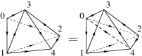
Figure 6: A retriangulation of a 3D complex.

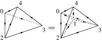
Figure 7: A retriangulation of another 3D complex.

The topological path integral that describes a 2+1D topologically ordered state with a gapped boundary can be constructed from a tensor set $T$ of two real and one complex tensors: $T=(w_{v_{0}},{d}_{e_{01}}^{v_{0}v_{1}},{C}_{v_{0}v_{1}v_{2}v_{3};\phi_{013}\phi_{123}}^{e_{01}e_{02}e_{03}e_{12}e_{13}e_{23};\phi_{012}\phi_{023}})$. The complex tensor ${C}_{v_{0}v_{1}v_{2}v_{3};\phi_{013}\phi_{123}}^{e_{01}e_{02}e_{03}e_{12}e_{13}e_{23};\phi_{012}\phi_{023}}$ can be associated with a tetrahedron, which has a branching structure (see Fig. 5). A branching structure is a choice of orientation of each edge in the complex so that there is no oriented loop on any triangle (see Fig. 5). Here the $v_{0}$ index is associated with the vertex-0, the $e_{01}$ index is associated with the edge-$01$, and the $\phi_{012}$ index is associated with the triangle-$012$. They represents the degrees of freedom on the vertices, edges, and the triangles.

Using the tensors, we can define the topological path integral on any 3-complex that has no boundary:

$$Z=\sum_{v_{0},\cdots;e_{01},\cdots;\phi_{012},\cdots} \prod_{\text{vertex}}w_{v_{0}}\prod_{\text{edge}}{d}_{e_{01}}^{v_{0}v_{1}}\times$$ (23)

$$\prod_{\text{tetra}}[{C}_{v_{0}v_{1}v_{2}v_{3};\phi_{013}\phi_{123}}^{e_{01}e_{02}e_{03}e_{12}e_{13}e_{23};\phi_{012}\phi_{023}}]^{s_{0123}}$$

where $\sum_{v_{0},\cdots;e_{01},\cdots;\phi_{012},\cdots}$ sums over all the vertex indices, the edge indices, and the face indices, $s_{0123}=1$ or $*$ depending on the orientation of tetrahedron (see Fig. 5). We want to choose the tensors $(w_{v_{0}}$, ${d}_{e_{01}}^{v_{0}v_{1}}$, ${C}_{v_{0}v_{1}v_{2}v_{3};\phi_{013}\phi_{123}}^{e_{01}e_{02}e_{03}e_{12}e_{13}e_{23};\phi_{012}\phi_{023}})$ such that the path integral is re-triangulation invariant. Such a topological path integral describes a topologically ordered state in 3-space-time dimensions and also define an topological order with gappable boundary.

On the complex $C^{3}_{N}$ with boundary: $B^{2}_{N^{\prime}}=\partial C^{3}_{N}$, the partition function is defined differently:

$$Z=\sum_{\{v_{i};e_{ij};\phi_{ijk}\}} \prod_{\text{vertex}\notin B^{2}_{N^{\prime}}}w_{v_{0}}\prod_{\text{edge}\notin B^{2}_{N^{\prime}}}{d}_{e_{01}}^{v_{0}v_{1}}\times$$ (24)

$$\prod_{\text{tetra}}[{C}_{v_{0}v_{1}v_{2}v_{3};\phi_{013}\phi_{123}}^{e_{01}e_{02}e_{03}e_{12}e_{13}e_{23};\phi_{012}\phi_{023}}]^{s_{0123}}$$

where $\sum_{v_{i};e_{ij};\phi_{ijk}}$ only sums over the vertex indices, the edge indices, and the face indices that are not on the boundary. The resulting $Z$ is actually a complex function of $v_{i}$’s, $e_{ij}$’s, and $\phi_{ijk}$’s on the boundary $B^{2}_{N^{\prime}}$: $Z=Z(\{v_{i};e_{ij};\phi_{ijk}\})$. Such a function is a vector in ${\cal H}_{B^{2}_{N^{\prime}}}$. We will denote such a vector as $|\Psi(C^{3}_{N})\rangle$.

We also note that the vertices and the edges are attached with the tensors $w_{v_{i}}$ and ${d}_{e_{01}}^{v_{0}v_{1}}$. But when we glue two boundaries together, those tensors $w_{v_{i}}$ and ${d}_{e_{ij}}^{v_{i}v_{j}}$ are added back. So the tensors $w_{v_{i}}$ and ${d}_{e_{ij}}^{v_{i}v_{j}}$ defines the inner product in the boundary Hilbert space ${\cal H}_{B^{2}_{N^{\prime}}}$. Therefore, we require $w_{v_{i}}$ and ${d}_{e_{ij}}^{v_{i}v_{j}}$ to satisfy the following unitary condition

$$w_{v_{i}}>0,\ \ \ {d}_{e_{ij}}^{v_{i}v_{j}}>0.$$ (25)

The invariance of $Z$ under the re-triangulation in Fig. 6 requires that

$$\ \ \ \sum_{\phi_{123}}{C}_{v_{0}v_{1}v_{2}v_{3};\phi_{013}\phi_{123}}^{e_{01}e_{02}e_{03}e_{12}e_{13}e_{23};\phi_{012}\phi_{023}}{C}_{v_{1}v_{2}v_{3}v_{4};\phi_{124}\phi_{234}}^{e_{12}e_{13}e_{14}e_{23}e_{24}e_{34};\phi_{123}\phi_{134}}$$

$$=\sum_{e_{04}}{d}_{e_{04}}^{v_{0}v_{4}}\sum_{\phi_{014}\phi_{024}\phi_{034}}{C}_{v_{0}v_{1}v_{2}v_{4};\phi_{014}\phi_{124}}^{e_{01}e_{02}e_{04}e_{12}e_{14}e_{24};\phi_{012}\phi_{024}}{C^{*}}_{v_{0}v_{1}v_{3}v_{4};\phi_{014}\phi_{134}}^{e_{01}e_{03}e_{04}e_{13}e_{14}e_{34};\phi_{013}\phi_{034}}{C}_{v_{0}v_{2}v_{3}v_{4};\phi_{024}\phi_{234}}^{e_{02}e_{03}e_{04}e_{23}e_{24}e_{34};\phi_{023}\phi_{034}}.$$ (26)

We would like to mention that there are other similar conditions for different choices of the branching structures. The branching structure of a tetrahedron affects the labeling of the vertices.

The invariance of $Z$ under the re-triangulation in Fig. 7 requires that

$${C}_{v_{0}v_{2}v_{3}v_{4};\phi_{024}\phi_{234}}^{e_{02}e_{03}e_{04}e_{23}e_{24}e_{34};\phi_{023}\phi_{034}}=\sum_{e_{01}e_{12}e_{13}e_{14},v_{1}}w_{v_{1}}{d}_{e_{01}}^{v_{0}v_{1}}{d}_{e_{12}}^{v_{1}v_{2}}{d}_{e_{13}}^{v_{1}v_{3}}{d}_{e_{14}}^{v_{1}v_{4}}\sum_{\phi_{012}\phi_{013}\phi_{014}\phi_{123}\phi_{124}\phi_{134}}$$ (27)

$$\ \ \ \ \ \ \ \ \ \ \ \ {C}_{v_{0}v_{1}v_{2}v_{3};\phi_{013}\phi_{123}}^{e_{01}e_{02}e_{03}e_{12}e_{13}e_{23};\phi_{012}\phi_{023}}{C^{*}}_{v_{0}v_{1}v_{2}v_{4};\phi_{014}\phi_{124}}^{e_{01}e_{02}e_{04}e_{12}e_{14}e_{24};\phi_{012}\phi_{024}}{C}_{v_{0}v_{1}v_{3}v_{4};\phi_{014}\phi_{134}}^{e_{01}e_{03}e_{04}e_{13}e_{14}e_{34};\phi_{013}\phi_{034}}{C}_{v_{1}v_{2}v_{3}v_{4};\phi_{124}\phi_{234}}^{e_{12}e_{13}e_{14}e_{23}e_{24}e_{34};\phi_{123}\phi_{134}}$$

Again there are other similar conditions for different choices of the branching structures.

The above two types of the conditions are sufficient for producing a topologically invariant partition function $Z$, which is nothing but the topological invariant for three manifolds introduced by Turaev and Viro.Turaev and Viro (1992) Again, two different solutions are regarded as equivalent if they produces the same topology-dependent partition function for any closed space-time.

It is also clear that the above construction of topological path integrals can be easily generalized to any other dimensions. This gives rise to a classification of topological orders with gappable boundary in higher dimensions.

Appendix C Quantum volume and its property

We have seen that when a tensor set, for example $T=(w_{v_{0}},{d}_{e_{01}}^{v_{0}v_{1}},{C}_{v_{0}v_{1}v_{2}v_{3};\phi_{013}\phi_{123}}^{e_{01}e_{02}e_{03}e_{12}e_{13}e_{23};\phi_{012}\phi_{023}})$, satisfy the conditions (B.2) and (27), its path integral on different space-time complexes will describe the same topological phase. If we change the tensors by a small amount, the tensor set will still describe the same topological phase for different space-time complexes. With such a more careful definition of path integral in term of the tensor set and the space-time complex $C_{N}^{d+1}$ with branching structure, we can define quantum volume more precisely.

For example, on 2+1D space-time complex $C^{3}_{N}$ with boundary $B^{2}_{N^{\prime}}$, the path integral produces a complex function $Z(\{v_{i};e_{ij};\phi_{ijk}\})$ with $\{v_{i};e_{ij};\phi_{ijk}\}\subset B^{2}_{N^{\prime}}$, which is a vector $|\Psi(C^{3}_{N})\rangle\in{\cal H}_{B^{2}_{N^{\prime}}}$ (see (24)). The inner product in ${\cal H}_{B^{2}_{N^{\prime}}}$ is defined through the weight-tensors $w_{v_{i}}$ ${d}_{e_{ij}}^{v_{i}v_{j}}$:

$$\langle\Psi|\Psi\rangle=\sum_{\{v_{i};e_{ij};\phi_{ijk}\}}\prod_{i}w_{v_{i}}\prod_{\langle ij\rangle}{d}_{e_{ij}}^{v_{i}v_{j}}|Z(\{v_{i};e_{ij};\phi_{ijk}\})|^{2}.$$ (28)

In this case the classical volume of $C^{3}_{N}$ is given by

$$V(C^{3}_{N},T)=\log\sqrt{\langle\Psi(C^{3}_{N},T)|\Psi(C^{3}_{N},T)\rangle}.$$ (29)

We can show that, for a many-body system described by tensor set $T$, its q-volume satisfies

$$\ \ \ \ |\Psi(C^{d+1}_{1}\cup C^{d+1}_{2})\rangle$$

$$={\rm Tr}_{\partial C^{d+1}_{1}\cap\partial C^{d+1}_{2}}[|\Psi(C^{d+1}_{1})\rangle\otimes|\Psi(C^{d+1}_{2})\rangle]$$ (30)

if the space-time complexes $C^{d+1}_{1}$ and $C^{d+1}_{2}$ only overlap on their boundaries. Here ${\rm Tr}_{\partial C^{d+1}_{1}\cap\partial C^{d+1}_{2}}$ traces over the internal degrees of freedom on the overlapped boundaries $\partial C^{d+1}_{1}\cap\partial C^{d+1}_{2}$ with the weighting tensors $w_{v_{1}}$, $d^{v_{1}v_{2}}_{e_{12}}$, etc for the internal simplices on the overlapped boundaries. In other words, we only traces over the indices for the simplices inside the overlapped boundaries (not those for the simplices on the boundary of the overlapped boundaries). The summation of each index is weighted by the corresponding weight tensor $w_{v_{1}}$ or $d^{v_{1}v_{2}}_{e_{12}}$ etc . (C) is a key property of the quantum volume.

References

- Wen (2003) X.-G. Wen, Phys. Rev. D 68, 065003 (2003), hep-th/0302201 .
- Levin and Wen (2006a) M. Levin and X.-G. Wen, Phys. Rev. B 73, 035122 (2006a), hep-th/0507118 .
- Wen (2013) X.-G. Wen, Chin. Phys. Lett. 30, 111101 (2013), arXiv:1305.1045 .
- You et al. (2014) Y.-Z. You, Y. BenTov, and C. Xu, (2014), arXiv:1402.4151 .
- You and Xu (2015) Y.-Z. You and C. Xu, Phys. Rev. B 91, 125147 (2015), arXiv:1412.4784 .
- Maldacena (1998) J. M. Maldacena, Adv. Theor. Math. Phys. 2, 231 (1998), hep-th/9711200 .
- Lee (2010) S.-S. Lee, Nucl. Phys. B 832, 567 (2010).
- Xu (2006) C. Xu, (2006), cond-mat/0602443 .
- Gu and Wen (2006) Z.-C. Gu and X.-G. Wen, (2006), gr-qc/0606100 .
- Gu and Wen (2012) Z.-C. Gu and X.-G. Wen, Nucl. Phys. B 863, 90 (2012), arXiv:0907.1203 .
- Witten (1989) E. Witten, Comm. Math. Phys. 121, 351 (1989).
- Atiyah (1988) M. Atiyah, Publications Mathématiques de lÍHÉS 68, 175–186 (1988).
- Wen (1990) X.-G. Wen, Int. J. Mod. Phys. B 4, 239 (1990).
- Wen and Niu (1990) X.-G. Wen and Q. Niu, Phys. Rev. B 41, 9377 (1990).
- Kitaev and Preskill (2006) A. Kitaev and J. Preskill, Phys. Rev. Lett. 96, 110404 (2006).
- Levin and Wen (2006b) M. Levin and X.-G. Wen, Phys. Rev. Lett. 96, 110405 (2006b), cond-mat/0510613 .
- Kong and Wen (2014) L. Kong and X.-G. Wen, (2014), arXiv:1405.5858 .
- Gu and Wen (2009) Z.-C. Gu and X.-G. Wen, Phys. Rev. B 80, 155131 (2009), arXiv:0903.1069 .
- Keski-Vakkuri and Wen (1993) E. Keski-Vakkuri and X.-G. Wen, Int. J. Mod. Phys. B 7, 4227 (1993).
- Zhang et al. (2012) Y. Zhang, T. Grover, A. Turner, M. Oshikawa, and A. Vishwanath, Phys. Rev. B 85, 235151 (2012), arXiv:1111.2342 .
- Costantino (2005) F. Costantino, Math. Z. 251, 427 (2005), math/0403014 .
- Chen et al. (2013) X. Chen, Z.-C. Gu, Z.-X. Liu, and X.-G. Wen, Phys. Rev. B 87, 155114 (2013), arXiv:1106.4772 .
- Chen et al. (2012) X. Chen, Z.-C. Gu, Z.-X. Liu, and X.-G. Wen, Science 338, 1604 (2012), arXiv:1301.0861 .
- Zeng and Wen (2015) B. Zeng and X.-G. Wen, Phys. Rev. B 91, 125121 (2015), arXiv:1406.5090 .
- Swingle and McGreevy (2016) B. Swingle and J. McGreevy, Phys. Rev. B 93, 045127 (2016), arXiv:1407.8203 .
- Turaev and Viro (1992) V. G. Turaev and O. Y. Viro, Topology 31, 865 (1992).
- Levin and Wen (2005) M. Levin and X.-G. Wen, Phys. Rev. B 71, 045110 (2005), cond-mat/0404617 .
- Kirillov.Jr. (2011) A. Kirillov.Jr., (2011), arXiv:1106.6033 .
- Balsam and Kirillov.Jr. (2012) B. Balsam and A. Kirillov.Jr., (2012), arXiv:1206.2308 .
- Chen et al. (2010) X. Chen, Z.-C. Gu, and X.-G. Wen, Phys. Rev. B 82, 155138 (2010), arXiv:1004.3835 .
- Verstraete and Cirac (2004) F. Verstraete and J. I. Cirac, (2004), cond-mat/0407066 .
- Levin and Nave (2007) M. Levin and C. P. Nave, Phys. Rev. Lett. 99, 120601 (2007).