Approximate ground states of the random-field Potts model from graph cuts

Abstract

While the ground-state problem for the random-field Ising model is polynomial, and can be solved using a number of well-known algorithms for maximum flow or graph cut, the analogue random-field Potts model corresponds to a multi-terminal flow problem that is known to be NP hard. Hence an efficient exact algorithm is very unlikely to exist. As we show here, it is nevertheless possible to use an embedding of binary degrees of freedom into the Potts spins in combination with graph-cut methods to solve the corresponding ground-state problem approximately in polynomial time. We benchmark this heuristic algorithm using a set of quasi-exact ground states found for small systems from long parallel tempering runs. For not too large number $q$ of Potts states, the method based on graph cuts finds the same solutions in a fraction of the time. We employ the new technique to analyze the breakup length of the random-field Potts model in two dimensions.

I Introduction

Due to its versatility, the Potts model is one of the central tools in statistical physics, in particular for the study of phase transitions and critical phenomena Wu (1982); Potts (1952). Its many physical realizations include soap froths, cellular tissues, grain growth, nucleation, as well as static and dynamic recrystallization. Disorder is inherent in such experimental systems and needs to be incorporated for their accurate description. Depending on the way the disorder couples to the system, this leads to the $q$-state random-bond or random-field Potts models. Experimentally, the latter is particularly relevant for describing magnetic grains, anisotropic orientational glasses, randomly diluted molecular crystals Binder and Reger (1992); Michel (1987), structural transitions in SrTiO₃ crystals Aharony et al. (1977), and phase transitions in type I antiferromagnets (such as NdSb, NdAs, CeAs) in a uniform field Domany et al. (1982). While the random-bond model has received substantial attention in the past and is relatively well understood in two (2d) Chen et al. (1992); Picco (1997); Berche and Chatelain (2004) as well as in three (3d) dimensions Chatelain et al. (2001); Berche et al. (2002); Hellmund and Janke (2003); Chatelain et al. (2005), little is known about the behavior of the random-field Potts model (RFPM). Due to the necessary quenched average over disorder and the slow relaxation resulting from the frustration introduced through the competition of exchange couplings and random fields (of strength $\Delta$), it is a difficult problem for analytical and numerical methods alike. Consequently, the nature of phases and the phase transitions in the $(q,\Delta)$-plane in different spatial dimensions $d$ are only partially understood, leaving many open questions for exploration.

There are only a few studies of the $q$-state RFPM in the literature Blankschtein et al. (1984); Nishimori (1983); Eichhorn and Binder (1995a, b, 1996); Reed (1985). These have primarily investigated the phase diagram in $(T,\Delta)$-space for different $q$ and $d$, where $T$ denotes temperature. For the pure model, the temperature-driven transitions are continuous for small $q\leq q_{c}$ and first-order for large $q>q_{c}$, with $q_{c}=4$ for the square-lattice model with nearest-neighbor interactions Duminil-Copin et al. (2017, 2016) and $q_{c}\approx 2.8$ for the simple-cubic lattice Hartmann (2005). It is well known that quenched disorder tends to soften first-order transitions Cardy (1999), and this has even been rigorously established for systems in two dimensions Aizenman and Wehr (1989). In the latter case, one hence must have $q_{c}\to\infty$, but in fact the RFPM does not show a finite-temperature ordering transition in $d=2$ and there are merely crossovers between ferromagnetic and paramagnetic states for finite systems, much alike to the behavior found for the 2d random-field Ising model (RFIM) Binder (1983a). For $d>2$, on the other hand, one would at least expect for $q_{c}$ to increase on coupling to the disorder. The only numerical studies of the problem are due to Eichhorn and Binder Eichhorn and Binder (1995a, b, 1996), who considered the case $q=3$ and $d=3$ using Monte Carlo simulations. They proposed a qualitative scenario in the $(q,d)$-plane which exhibited a shift of the tri-critical curves $q_{c}(d)$ to higher values, consistent with the mean-field predictions of Blankschtein et al. Blankschtein et al. (1984). The simulation results for $q=3$ indicated a continuous transition for the considered disorder strength. It is clear, however, that these simulations, which date back to before the advent of modern simulation techniques for disordered systems such as parallel tempering Hukushima and Nemoto (1996), might be affected by equilibration problems and strong corrections to finite-size scaling. Additionally, the question of whether a softening of discontinuous transitions occurs for all strengths $\Delta$ of the random fields or only above a certain threshold has not been addressed to date.

A related system is the random-field Ising model (RFIM) Nattermann (1997) which, up to a rescaling, can be mapped onto the RFPM for $q=2$, see the discussion in Sec. II. Although this system was studied extensively over the past decades, it is only recently that large-scale numerical studies were able to settle a number of important questions for this problem Fytas and Martín-Mayor (2013); Fytas et al. (2016), such as the number (and values) of independent exponents, the universality of transitions with respect to the coupling distribution and the issue of dimensional reduction Parisi and Sourlas (1979). An important feature of the renormalization-group (RG) treatment of this system is that the RG fixed point that controls the disordered transition is located at $T=0$ Bray and Moore (1985). As a consequence, a systematic study of ground states in this case allows to extract the critical exponents of the transition at finite temperature so it exists. It is a fortunate coincidence that the problem of finding the ground state for an RFIM sample can be mapped to a maximum-flow problem that is in P Anglès d’Auriac et al. (1985), i.e., there exist algorithms that solve it in a time that grows as a polynomial in the size of the system, including the Ford-Fulkerson algorithm of augmenting paths Ford Jr and Fulkerson (2015), the Goldberg-Tarjan push-relabel method Goldberg and Tarjan (1988), or variants thereof Boykov and Kolmogorov (2004). In the last few years, we have acquired significant knowledge about the ground-state properties of the RFIM Shrivastav et al. (2011, 2014a, 2014b); Banerjee et al. (2014); Stevenson and Weigel (2011a, b). The situation is different, however, for the case of the RFPM with $q>2$ which corresponds to a multi-terminal flow or, equivalently, graph cut (GC) problem that is known to be NP hard Boykov et al. (2001); Anglès d’Auriac et al. (1985). Still, as was shown by Boykov et al. Boykov et al. (2001), solutions to such multi-terminal flow problems can be efficiently approximated using an embedding of binary degrees of freedom into the states with more than two labels.

In the present paper, we undertake a first exploratory study into determining ground states of the $q$-state RFPM using graph-cut methods. By comparing the results of the heuristic GC algorithm to those of parallel tempering (PT) simulations systematically tuned to yield ground states for small systems in 2d with very high success probabilities, we establish that the GC approach yields reasonable estimates of ground states for the $q$-state RFPM. The run times of the GC approach are significantly smaller than those of the PT simulations, and they scale linearly with the system size as well as the number of states, allowing us to study large system sizes.

The rest of the paper is organized as follows. In Sec. II, we describe the $q$-state random field Potts model, the graph cut method, and the parallel tempering approach. Section III provides detailed comparisons between (quasi) exact ground states obtained using PT and approximate ground states found using the GC method. We also demonstrate here that GC provides a good approximation to the ground states, especially for small $q$. In Sec. IV we apply the GC method to study the breakup length for the $q=3$ and $q=4$ RFPM in two dimensions. Finally, in Sec. V, we conclude this paper with a summary and discussion.

II Model and Methodology

In the following, we describe the variant of the RFPM studied here and introduce two numerical approaches for determining ground states of samples, the graph-cut method and parallel tempering.

II.1 Random Field Potts Model

The ferromagnetic $q$-states Potts model is described by the Hamiltonian Wu (1982)

$${\cal H}=-J\sum_{\langle ij\rangle}\delta_{s_{i},s_{j}},$$ (1)

where the $s_{i}\in\{0,1,\ldots,q-1\}$ are the Potts spins, $\langle ij\rangle$ denotes summation over nearest neighbors only, and $J>0$ is a (ferromagnetic) coupling constant. For the purposes of the present study, we consider systems on square and simple-cubic lattices with periodic boundary conditions. The coupling of the spins to random fields can take a variety of different forms Blankschtein et al. (1984); Eichhorn and Binder (1996); Goldschmidt and Xu (1985). A symmetric coupling of continuous fields can be expressed as Blankschtein et al. (1984):

$$\mathcal{H}=-J\sum_{\left<ij\right>}\delta_{s_{i},s_{j}}-\sum_{i}\sum_{\alpha=0}^{q-1}h_{i}^{\alpha}\delta_{s_{i},\alpha},$$ (2)

where $\{h_{i}^{\alpha}\}$ denotes the quenched random field at site $i$, acting on state $\alpha$. Hence, in this model, the random field at each site has $q$ components, and we take each of these to follow a normal distribution. To separate the disorder strength from the random instance we define $h_{i}^{\alpha}=\Delta\epsilon_{i}^{\alpha}$ and $\epsilon_{i}^{\alpha}$ are then drawn from a standard normal distribution, i.e.,

$$P(\epsilon_{i}^{\alpha})=\frac{1}{\sqrt{2\pi}}\exp\left(-{\epsilon_{i}^{\alpha}}^{2}/2\right).$$ (3)

For the case $q=2$, the Hamiltonian (2) has two different random fields $h_{i}^{0}\equiv h_{i}^{+}$ and $h_{i}^{1}\equiv h_{i}^{-}$ for the two spin orientations, in contrast to the usual definition of the RFIM Nattermann (1997). As is easily seen, however, Eq. (2) in this case can be written as

$$\mathcal{H}=-\frac{J}{2}\sum_{\left<ij\right>}[\sigma_{i}\sigma_{j}+1]-\frac{1}{2}\sum_{i}[(h_{i}^{+}-h_{i}^{-})\sigma_{i}+(h_{i}^{+}+h_{i}^{-})],$$ (4)

where $\sigma_{i}=\pm 1$ are Ising spins. It is hence clear that, up to a constant shift, the $q=2$ RFPM of Eq. (2) and with the distribution (3) at coupling constant $J$ and random field $\Delta$ is equivalent to the RFIM at coupling $J/2$ and field strength $\Delta/\sqrt{2}$.

An alternative model with discrete distribution of the disorder is given by Eichhorn and Binder (1996); Goldschmidt and Xu (1985)

$$\mathcal{H}=-J\sum_{\left<ij\right>}\delta_{s_{i},s_{j}}-\Delta\sum_{i}\delta_{s_{i},h_{i}}.$$ (5)

Here, the quenched random variables $h_{i}$ are chosen uniformly from the set $\{0,1,\ldots,q-1\}$, i.e.,

$$P(h_{i})=\frac{1}{q}\sum_{\alpha=0}^{q-1}\delta_{h_{i},\alpha}.$$ (6)

Thus the distribution of random fields is discrete, and couples to any one of the $q$ spin states with equal probability. We note that for the continuous form (2) we expect a unique ground state, while the alternative (5) might admit (extensive) degeneracies, in particular for rational choice of $\Delta$. While the discreteness of the form (5) might have certain advantages for the efficient implementation of simulation codes, we would like to avoid the possible subtleties associated with degeneracies, and we will hence use the form (2) here.

II.2 Graph Cut Method

While the ground-state problem of the RFPM is NP hard and so an exact solution is out of reach, an efficient approximation algorithm has been developed in the context of applications of the Potts model (and related systems) in computer vision Boykov et al. (2001). The method is tailored for a general energy function of the form

$$E(\{s_{i}\})=\sum_{i,j}V_{ij}(s_{i},s_{j})+\sum_{i}D_{i}(s_{i}),$$ (7)

where in the original application $s_{i}$ would have referred to the color label of the pixels of a (planar) image, but the interaction matrix $V_{ij}$ can be such that also more general graphs and three-dimensional systems can be modeled. The RFPM Hamiltonian (2) is clearly a special case of this general form. Each site $i$ is assigned a label $s_{i}\in\{0,1,\ldots,q-1\}$. The function $V_{ij}(s_{i},s_{j})$ gives the cost of assigning labels $s_{i}$ and $s_{j}$ to the sites $i$ and $j$, while the function $D_{i}$ measures the penalty (or cost) of assigning the label $s_{i}$ to site $i$. The basic approach taken in Ref. Boykov et al. (2001) is to consider constraint optimization problems derived from Eq. (7) in such a way that the $q$ labels are reduced to an effective two-label problem. As this is then equivalent to (a slight generalization of) the RFIM, a ground state for this constraint problem can be determined exactly and in polynomial time using the established min-cut/max-flow algorithms. This idea is in the same spirit as the embedding of Ising variables used in combination with minimum-weight perfect matching in dealing with continuous-spin glasses on planar lattices Weigel and Gingras (2006); Weigel (2007).

The two approaches of this type proposed in Ref. Boykov et al. (2001) are the $\alpha$-$\beta$-swap and the $\alpha$-expansion moves. For the $\alpha$-$\beta$-swap one picks two labels $\alpha\neq\beta\in\{0,1,\ldots,q-1\}$ and freezes all labels apart from $\alpha$ and $\beta$. Under this constraint, the problem (7) is equivalent to a two-label problem on the sites with labels $\alpha$ or $\beta$ that can be solved by min-cut/max-flow. This step is repeated for each pair of labels, resulting in a cycle of $q(q-1)\approx q^{2}$ steps. For the $\alpha$-expansion move one picks a label $\alpha$ which is then frozen. The remaining pixels are given the alternative of either keeping their current label or being flipped into the $\alpha$ state, which is again a binary choice, and the resulting constraint problem can be solved by min-cut/max-flow. A cycle of the $\alpha$-expansion takes $q$ steps. Independent of which of the two algorithms is used, cycles are repeated until the configurations do not change any further, and the methods have converged to a local minimum.

While these algorithms are not exact and are hence not guaranteed to find ground states, they have been reported to yield excellent approximations to the ground states and are widely used in computer vision. For the $\alpha$-expansion move, it is possible to derive an upper bound on the energy of the local minima found, which is given by

$$E(\hat{f})\leq 2cE(f^{*}),\quad\mbox{where}\quad c=\frac{{\rm max}_{s_{i}\neq s_{j}}V(s_{i},s_{j})}{{\rm min}_{s_{i}\neq s_{j}}V(s_{i},s_{j})},$$ (8)

$\hat{f}$ is the state returned by the $\alpha$-expansion move, and $f^{*}$ is the global optimum. For the Potts model, $V_{ij}(s_{i},s_{j})\equiv-J\delta_{s_{i},s_{j}}$, yielding $c=1$. So the expansion move provides a local minimum within a factor of two of the global minimum. To check the effectiveness of their algorithms, the authors of Ref. Boykov et al. (2001) experimented on a variety of computer vision problems such as image restoration with multiple labels, stereo and motion. These problems are solved by computing a minimum cost multi-way cut on the graph. A comparison of their results with known ground states revealed 98% accuracy Boykov et al. (2001). The method has not previously been applied to the RFPM, and to benchmark it there, we need a collection of samples with known ground states. For this purpose, we use the replica exchange or parallel tempering (PT) method, which can be used to find exact ground states with high probability for small systems.

II.3 Parallel Tempering

Table 1: Optimized values of $\eta$ according to Eq. (10) and the number of temperature replicas $N_{T}$ for different lattices with $L^{2}$ spins used in the parallel tempering.

$L$	8	12	16	20	24	32	40
$N_{T}$	16	16	16	16	16	32	32
$\eta$	1.13	1.13	1.13	1.13	1.13	1.14	1.14

Ground states of RFPM samples could be generated via exact enumeration of states. Due to their exponential number $\sim q^{N}$ this only works for the tiniest of systems, however. While this situation could possibly be improved with the use of branch-and-cut techniques De Simone et al. (1995), we do not follow this approach here and instead revert to stochastic approximation schemes based on Markov chain Monte Carlo simulations. Simple Monte Carlo at a fixed low or even zero temperature will not lead to ground states. The RFPM has a complicated free energy landscape with many minima and maxima. These metastable states trap the evolving system and impede the relaxation to the ground state. Any reasonable Monte Carlo sampling therefore has to overcome energy barriers and cross from one basin to another to reach the global minimum. Established approaches to achieve this are simulated annealing Kirkpatrick et al. (1983) and parallel tempering Geyer (1991); Hukushima and Nemoto (1996). It has been shown that among the Monte Carlo methods parallel tempering consistently outperforms simulated annealing as a tool for ground-state searches in disordered systems Wang et al. (2015) . We will hence focus on parallel tempering (PT).

Consider $N_{T}$ initially non-interacting replicas of the system at distinct temperatures. In PT each replica is evolved at its temperature $T_{m}$ using canonical Monte Carlo, for example employing the single spin-flip Metropolis method Landau and Binder (2015). In an additional step, replicas with neighboring temperatures are exchanged with the probability

$$P_{\rm ex}=\min\left[1,e^{(\beta_{m}-\beta_{m+1})(E_{m}-E_{m+1})}\right],$$ (9)

where $\beta_{m}=1/k_{B}T_{m}$ and $E_{m}$ denotes the configurational energy of the $m$th replica. This scheme couples the replicas and allows copies that are trapped in metastable states at low temperatures to escape to high temperatures via successive exchanges with neighboring copies, where they can more easily relax to then return via the same random walk in temperature space to low temperatures, typically exploring a different basin.

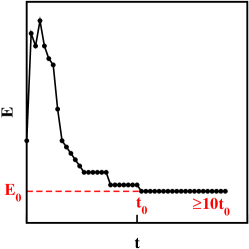
Figure 1: Schematic diagram showing the variation of $E$ with time $t$ in the PT runs (in MC steps). The first occurrence of the minimum energy $E_{0}$ is at onset time $t=t_{0}$. The corresponding state is accepted as a ground state if no lower energy is found up to $t\geq 10t_{0}$.

The most delicate aspect of PT relates to the choice of the number and spacing of the replicas in temperature space. Clearly, neighboring temperatures must be close enough such that the acceptance probabilities (9) are appreciable, which essentially means that the energy histograms at neighboring temperatures must have sufficient overlap Bittner et al. (2008). On the other hand, too many replicas with consequently high acceptance rates of swaps are also not ideal as this slows down the random walk in temperature space through smaller and smaller temperature steps. A number of different protocols have been suggested for choosing the optimal set $\{T_{m}\}$ Katzgraber et al. (2006); Bittner et al. (2008); Kofke (2002); Kone and Kofke (2005); Predescu et al. (2004); Sabo et al. (2008); Neirotti et al. (2000); Calvo (2005); Brenner et al. (2007). Here we use a heuristic scheme based on a generalization of the widely used geometric progression of temperatures Katzgraber (2009), and choose the temperatures according to

$$T_{m}=m^{\eta}T_{\rm norm}+T_{\rm min},\quad\mbox{where}\quad T_{\rm norm}=\frac{T_{\rm max}-T_{\rm min}}{(N_{T}-1)^{\eta}}.$$ (10)

The choice of the maximum and minimum temperatures $T_{\rm max}$ and $T_{\rm min}$ is guided by the need to select a sufficiently high $T_{\rm max}$ to ensure good relaxation of replicas that arrive there, and (in our case of using PT as a global optimization algorithm) a sufficiently low $T_{\rm min}$ to allow us to find ground states. From preliminary tests, we found that $T_{\rm max}=1.5$ and $T_{\rm min}=0.2$ are sufficient for our purposes. We first determine the number of replicas $N_{T}$ by generating the corresponding sequence of temperatures for $\eta=1$. If a test run shows overall low swap acceptance rates, we increase $N_{T}$. The adjustable parameter $\eta$ is found recursively as follows: (1) The simulations are performed for a chosen value of $\eta$ and the set of temperatures $\{T_{m}\}$ determined using Eq. (10); (2) The tunneling time, i.e., the average time for a replica to travel from the lowest to the highest temperature and back, is measured in a test simulation ; (3) Steps 1 and 2 are repeated for a modified value of $\eta$. The value of $\eta$ which minimizes the tunneling time is selected to yield the optimal set $\{T_{m}\}$. The values of $\eta$ and $N_{T}$ for a lattice of lateral size $L$, after this optimization protocol, are listed in Table 1 . For simplicity we used the same parameters for different numbers of states $q$, although for best performance these cases should be separately optimized.

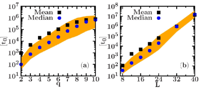
Figure 2: Disorder-averaged onset times $t_{0}$ for finding the ground states of the $d=2$ RFPM using parallel tempering. The data is plotted on a linear-log scale as a function of (a) the number of Potts states $q$ for $L=16$, and (b) the system size $L$ for $q=3$. The data are averaged over $1536$ realizations of quenched random fields according to Eq. (3) with $\Delta=1$. The shaded area shows the range that contains the onset times for 66% of the samples.

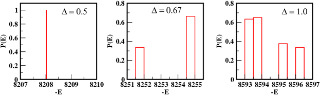
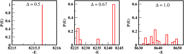
Figure 3: Energy histograms of final states obtained from GC for the $q=3$ RFPM (top row) and the $q=4$ RFPM (bottom row) on a $64^{2}$ lattice. The histograms are obtained from 10 000 initial configurations $\{s_{i}\}$ for a fixed disorder configuration $\{\epsilon_{i}^{\alpha}\}$.

As a realization of Markov chain Monte Carlo that satisfies ergodicity and detailed balance, PT is guaranteed to converge to the equilibrium distribution Landau and Binder (2015). Nevertheless, while it performs much better than local updates alone, for systems with complex free-energy landscapes such as the RFPM the equilibration times can still be very long, and they increase steeply with system size and with lowering $T_{\mathrm{min}}$. For not too large systems, however, we are able to find ground states for the overwhelming majority of samples. To ensure this, we rely on the following bootstrapping procedure:

1. We run all samples for given $L$ and $q$ for some initial time chosen to ensure equilibration of an average sample (determined, for example, by measuring the average tunneling time).

2. For each sample, we determine the onset time $t_{0}=t_{0}(\{h_{i}^{\alpha}\})$, i.e., the time when the lowest energy seen in the whole run is observed first.

3. We re-run each sample with a runtime of $t(\{h_{i}^{\alpha}\})=10\times t_{0}(\{h_{i}^{\alpha}\})$.

4. For samples where a new, lower state is found in the extended runs, we repeat this procedure until the condition $t=10\times t_{0}$ is met.

This procedure is illustrated in Fig. 1. It is highly reliable in finding ground states, and we estimate the failure probability for the system sizes considered to be of the order of 1 in 1000. For none or the samples considered here was a state lower than the reference state determined from the procedure above found in any of the other runs (PT or GC).

We performed such simulations for system sizes $8\leq L\leq 40$ and number of states $2\leq q\leq 10$ for 1536 configurations of the random fields each. The resulting average and median onset times of the ground states are shown in Fig. 2. The shaded area indicates the level of disorder fluctuations. These plots are shown on a linear-log scale. In Fig. 2(a), we observe that $t_{0}$ increases slightly slower than exponentially with the number of Potts states $q$. In Fig. 2(b), we observe an exponential increase of $t_{0}$ for system sizes $L\geq 16$. This is what we expect for any process geared towards ensuring exact ground states as the problem is NP hard. As the mean values are larger than the medians, the distribution is asymmetrical and tail-heavy for all values of $q$ and $L$.

III Benchmarks

We first consider the behavior of the GC method in its own right before turning to a detailed comparison of this technique to the PT method. The bulk of our runs were performed in two dimensions, but some of the timing runs discussed in Sec. III.3 were repeated for cubic lattices.

III.1 Approximate ground states from GC

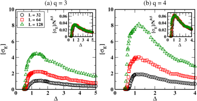
Figure 4: Variation of the standard deviation of energy $[\sigma_{E}]$ from runs of the GC method as a function of disorder amplitude $\Delta$ for the $d=2$ RFPM with (a) $q=3$, and (b) $q=4$. All data are averaged over 100 disorder realizations $\{\epsilon_{i}^{\alpha}\}$, and 1000 initial states $\{s_{i}\}$ for each disorder realization. Clearly, $[\sigma_{E}]$ grows with lattice size $L$, and also with number of states $q$. The scaled data in the insets demonstrate that $[\sigma_{E}]\sim\sqrt{N}=L$, i.e., there are no critical fluctuations in this range of $\Delta$-values.

Let us begin by testing the final states obtained via graph cuts in the RFPM. We fix the disorder configuration $\{\epsilon_{i}^{\alpha}\}$ and obtain the final states from several runs of GC for different initial spin configurations $\{s_{i}\}$. The top row of Fig. 3 shows energy histograms of these states for the $q=3$ RFPM. The simulations are performed on a $64^{2}$ lattice with $10\,000$ initial conditions. For $\Delta=0.5$, the system always converges to the same energy state. Hence the histogram shows a sharp peak corresponding to that energy state. As we increase the disorder strength $\Delta$, the distribution spreads over multiple energy states. The bottom row of Fig. 3 shows similar histograms for the $q=4$ RFPM, which are even wider. Therefore, the GC method is not guaranteed to yield a ground state of the RFPM. This is corroborated by a comparison of the actual states found to the true ground states as discussed in Sec. III.2 below.

To quantify the energy spread in the histogram, we determine the standard deviation in energy,

$$\sigma_{E}=\left(\left<E^{2}\right>-\left<E\right>^{2}\right)^{1/2},$$ (11)

where the angular brackets $\left<\cdot\right>$ denote an average over different initial conditions for a fixed disorder realization. A further average over independent disorder configurations yields the disorder-averaged quantity $\left[\sigma_{E}\right]$. In Fig. 4, we plot $\left[\sigma_{E}\right]$ vs. $\Delta$ on a $d=2$ lattice ($L\times L\equiv N$) for $L=32$, $64$, $128$. The data has been averaged over 100 disorder realizations, and 1000 initial states for each disorder configuration. The energy spread grows with $L$. To understand this dependence, we plot $\left[\sigma_{E}\right]/\sqrt{N}$ vs. $\Delta$ in the insets. The data collapse shows that $\left[\sigma_{E}\right]\sim\sqrt{N}$, demonstrating the absence of critical fluctuations. The relative fluctuations in the energy, $\left[\sigma_{E}\right]/\left<E\right>\sim N^{-1/2}$, vanish in the thermodynamic limit. In the limit $\Delta\rightarrow\infty$, we can neglect the exchange term in Eq. (2), which yields $\left<E\right>=-N\Delta$ and $\left<E^{2}\right>=N^{2}\Delta^{2}$, i.e., $\sigma_{E}\rightarrow 0$ as $\Delta\rightarrow\infty$.

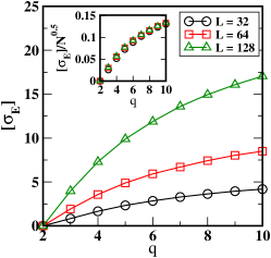
Figure 5: Plot of $[\sigma_{E}]$ vs. $q$ for the $d=2$ RFPM with $\Delta=1.0$, and indicated lattice sizes. The statistics is the same as in Fig. 4. The spread in energy of the GC states increases with $q$. The inset shows that $[\sigma_{E}]\sim\sqrt{N}=L$.

The $q$-dependence of the energy spread can be understood from Fig. 5, where we plot $\left[\sigma_{E}\right]$ vs. $q$. The data sets correspond to $\Delta=1.0$. The increase in number of metastable states with $q$ implies that the GC approach becomes worse in terms of the quality of the energy minima. The inset of this figure again confirms $\sigma_{E}\sim\sqrt{N}$.

III.2 Comparisons with PT

Having established a database of samples for which the ground states are known with very high probability through the PT procedure described in Sec. II.3, it is possible to benchmark the GC method against quasi-exact results as well as against PT runs. In Fig. 6 we show the average success probability $P_{0}$, i.e., the disorder-averaged probability of finding the actual ground state from the GC technique as a function of $q$ (left panel) and $L$ (right panel), respectively. These probabilities decay strongly with increasing $q$ and $L$, and both plots are consistent with an exponential behavior that should be expected when applying a polynomial-time algorithm to an NP hard problem. Note, however, that the values of $P_{0}$ are for GC runs with a single initial configuration that take only fractions of a second (see the discussion of run times below in Sec. III.3). In real applications one would normally perform runs for many initial conditions and pick the state of lowest energy. This approach is a generic method of improving global optimization algorithms Weigel (2007); Khoshbakht and Weigel (2017). The success probability of a sequence of $m$ runs with different initial conditions follows an exponential,

$$P_{s}(\{h_{i}^{\alpha}\})=1-[1-P_{0}(\{h_{i}^{\alpha}\})]^{m}.$$ (12)

Hence for a certain target success probability $P_{s}$, the required number of runs follows from

$$m(\{h_{i}^{\alpha}\})=\ln[1-P_{s}]/\ln[1-P_{0}(\{h_{i}^{\alpha}\})],$$ (13)

where we write $m(\{h_{i}^{\alpha}\})$ and $P_{n}(\{h_{i}^{\alpha}\})$ to indicate that this is for a single disorder realization. With $P_{0}=0.00187$ for $q=3$ and $L=40$ shown in the right panel of Fig. 6, for example, using $m=2460$ runs ensures $P_{s}=0.99$ .

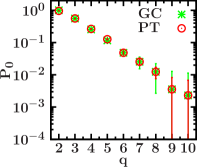
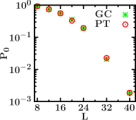
Figure 6: Disorder-averaged success probability of finding the ground state from GC and PT runs for 2d RFPM as a function of $q$ (left panel, $L=16$) and $L$ (right panel, $q=3$). The GC data correspond to one initial state per disorder sample, while the run time in PT was adapted to yield exactly the same average success probability as the corresponding GC run (see main text). All data are averaged over 1536 configurations of the random fields.

In order to compare the performance of GC and PT, we tune the latter via the number of Monte Carlo steps used to yield the same average success probability (on the same set of samples) as GC. This can be easily achieved without additional calculations from the onset times determined in Sec. II.3: the number of steps $t^{\ast}$ for all runs is chosen such that the fraction $n(t^{\ast})/N_{s}$ of samples with $t_{0}<t^{\ast}$ exactly equals the success probability $P_{0}$ observed for GC, where $N_{s}=1536$ is the total number of samples studied. This is illustrated by the data points for PT also shown in Fig. 6 that fall on top of the results for GC.

While the success probabilities of one GC run and the PT simulation with $t^{\ast}$ steps are identical, this does not imply that both methods find the same states in case they do not arrive at ground states. To quantify the quality of approximation in these cases, we consider the relative excess energy of the minimum energies returned by both algorithms above the ground state,

$$\varepsilon=\frac{E_{\mathrm{min}}-E_{0}}{E_{0}}.$$ (14)

This quantity, which we call accuracy, is shown in Fig. 7 which reveals that the accuracy at the same success probability is approximately comparable as a function of $L$ and for $q=3$ in the regime considered, but the approximation provided by the GC approach appears to more rapidly deteriorate as $q$ is increased than that of PT. Note that $[\epsilon]=0$ for GC at $q=2$ as this method finds exact ground states for the RFIM. We also considered the overlap,

$$O=\frac{1}{N}\sum_{i=1}^{N}\delta_{s_{i},s_{i}^{0}}$$ (15)

of the minimum-energy configurations $\{s_{i}\}$ found with the true ground states $\{s_{i}^{0}\}$. This is shown in Fig. 8. As for the accuracy, the overlap decreases quickly with increasing $q$. For $q=3$, on the other hand, overlaps are generally high and decrease only moderately with $L$. For the GC approach, there is a tendency of the decay to settle for $L\gtrsim 32$, promising to provide states of high similarity to the true ground states even for larger system sizes.

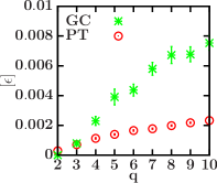
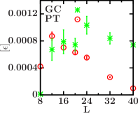
Figure 7: Accuracy $[\varepsilon]$ defined in Eq. (14) of GC and PT runs for the $d=2$ RFPM as a function of $q$ (left panel, $L=16$) and $L$ (right panel, $q=3$), respectively. Both methods are tuned to have the same success probabilities, as shown in Fig. 6. The data are averaged over 1536 disorder realizations with $\Delta=1.0$.

III.3 Run times and computational complexity

Let us now discuss the time taken by the GC method to find an approximate ground state of the RFPM. We measure the CPU time $r$ (in seconds) that the $\alpha$-expansion variant of GC used here takes to reach its final state. We ran our codes on an IBM cluster with 2.67 GHz Intel Xeon processors. The simulations are performed for $\Delta=1.0$, and $r$ is averaged over 1000 disorder samples. Fig. 9 (top row) shows the run time $[r]$ for the $q$-state RFPM in $d=2$. We plot $[r]$ as a function of (a) the total number of spins $N=L^{2}$ for $q=10$, $50$, $100$; and (b) $q$ for $L=128$, $256$. The solid lines are power-law fits with the specified exponent. Clearly, $[r]$ is linear in $N$ and $q$ for the $q$-state RFPM. This is in line with the general discussion of the time complexity of the method given in Sec. II.2. A similar analysis for the RFPM in three dimensions is summarized in the bottom row of Fig. 9 which shows that also in this case the run time is approximately linear with respect to $N$ and $q$.

We finally consider the scaling of run times of the GC and PT techniques with the latter scaled to achieve the same success probability in finding ground states as the former. We compare the timings of the GC method to two different implementations of PT, one regular CPU code and a highly optimized implementation on graphics processing units (GPUs) Weigel (2018); Kumar et al. . The GPU code is about 128 times faster than the CPU implementation. The corresponding run times for the two-dimensional RFPM are shown in Fig. 10, using an Nvidia GTX1060 GPU. The times for the GC approach depend linearly on $q$ and $N=L^{2}$ to a very good approximation as already seen above. The CPU variant of PT is always significantly slower that GC at the same success probability. The GPU code is slightly faster than GC for small systems, but for larger system sizes the GC approach becomes more favorable as PT shows a clearly superlinear increase of run times there. For the system sizes probably used in practical studies that are significantly larger than the sizes $L\leq 40$ considered with quasi-exact ground states here, we expect a substantial advantage for GC over PT.

IV Scaling of the breakup length

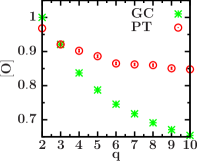
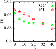
Figure 8: Average overlap $[O]$ [see Eq. (15)] of the states returned by GC and PT, respectively, with the true ground states for the $d=2$ RFPM as a function of $q$ for $L=16$ (left) and $L$ for $q=3$ (right), respectively. The averaging is done over 1536 disorder realizations with $\Delta=1.0$.

We finally consider an application of the methods outlined above to exploring the physical properties of the RFPM in two dimensions. Given the absence of finite-temperature ordering in the 2d RFIM Binder (1983b), it seems fairly clear that the RFPM also does not admit order at $T>0$ Aizenman and Wehr (1989); Blankschtein et al. (1984). Instead, one expects the presence of ferromagnetic domains that break up at a length scale $L_{b}(\Delta)$ similar to what is observed for the RFIM Binder (1983b); Seppälä et al. (1998). At very small disorder, the ground state approaches a purely ferromagnetic state for all but the largest system sizes, while at large disorder the ground state breaks into domains of $q$ labels. To determine $L_{b}$, we follow Ref. Seppälä et al. (1998) and count the fraction of samples with a purely ferromagnetic ground state, defining the probability $P_{\mathrm{FM}}(L,\Delta)$. This quantity is shown in Fig. 11(a) as determined from GC for $q=3$ and a number of different lattice sizes $L$. The breakup length $L_{b}$ can then be defined from the condition $P_{\mathrm{FM}}(L,\Delta)=0.5$ Seppälä et al. (1998). A plot of $L_{b}$ vs. $1/\Delta$ is shown for the cases $q=2$, $3$, and $4$ in Fig. 11(b) using a semi-logarithmic scale. We find that fits of the simple exponential form

$$L_{b}\sim\exp(A/\Delta)$$ (16)

to the data work well, and we arrive at $A=3.6\pm 0.03$ as a $q$-independent constant that depends only on the disorder distribution. We note that this scaling is not consistent with that proposed in Refs. Binder (1983b); Seppälä et al. (1998) for the RFIM, but it is in line with what was found in numerical simulations of the RFIM in Ref. Shrivastav et al. (2014a). The reason for this discrepancy might be the presence of only a rather weak curvature in a plot of the type of Fig. 11(b), and one might need to go to rather small $\Delta$ to see the asymptotic behavior.

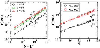
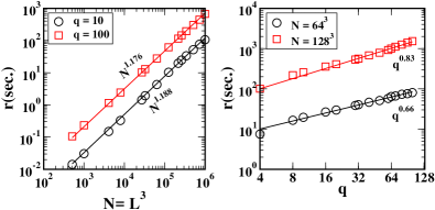
Figure 9: Disorder-averaged run time $[r]$ (in CPU sec.) for determining the final state by the application of the $\alpha$-expansion GC method to the RFPM in two dimensions (top row) and three dimensions (bottom row) as a function of the number of spins $N=L^{d}$ and the number of states $q$, respectively. The data are averaged over 1000 disorder realizations with $\Delta=1.0$. The solid lines are power-law fits with the specified exponents, and demonstrate that the run time is linear in $N$ and approximately linear in $q$.

V Summary and Discussion

The problem of finding the ground state of the $q$-state random field Potts model (RFPM) corresponds to a multi-terminal flow problem that is known to be NP hard. Although this model has many physical realizations, the unavailability of suitable methods has been an impediment in the study of the RFPM. The energy functions of such complex spin systems have several deep minima separated by high-energy barriers which grow exponentially with the system size $N$. In this paper, we have explored the utility of a graph-cut method proposed by Boykov et al. Boykov et al. (2001) for finding approximate ground states of the RFPM. The approach has the advantage of converging to the final state in polynomial time. However, there is no guarantee that the states found are ground states for the $q$-state RFPM when $q\geq 3$. Therefore, it is crucial to benchmark the quality of this approximation.

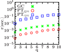
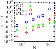
Figure 10: Disorder-averaged run time $[r]$ of the GC method for the 2d RFPM as compared to CPU and GPU implementations of the PT method tuned to achieve the same success probability as a function of $q$ (left panel, $N=16^{2}$) and as a function of $N=L^{2}$ (right panel, $q=3$).

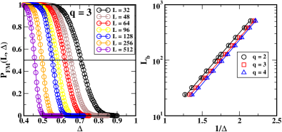
Figure 11: Left panel: Disorder-averaged probability $P_{\mathrm{FM}}(L,\Delta)$ of samples of the 2d $q=3$ RFPM to have purely ferromagnetic ground states. The data are averaged over 10 000 disorder realizations for $L\leq 128$ and 5 000 realizations for $L=256$ and $512$. Right panel: The breakup length scale $L_{b}$, defined as the system size $L$ where $P_{\mathrm{FM}}(L,\Delta)=0.5$, versus the inverse random-field strength $1/\Delta$ for $q=2$, $3$, and $4$. The solid lines show fits of the functional form $L_{b}\sim e^{A/\Delta}$ to the data, where $A=3.6\pm 0.03$.

We have used a carefully tuned set of parallel tempering simulations for creating a benchmark set of instances for which the ground states are known with an exceedingly high probability. These allowed to gauge the success probabilities of finding ground states for the graph-cut method and for short parallel tempering simulations. It is found that as a function of system size $L$ the quality of the states returned by graph-cut and parallel tempering techniques is quite similar for small $q$ and system sizes up to $40\times 40$ spins. For larger systems and $q=3$, there is a tendency of the graph-cut approach to yield a better approximation. For increasing values of $q$, on the other hand, the quality of graph-cut results deteriorates rather quickly. The actual time required for a run of the graph-cut method for small $L$ and different values of $q$ is much smaller than that of a corresponding parallel tempering run performed on CPU and comparable to that of a highly efficient GPU implementation of parallel tempering. For larger system sizes there is a crossover and the graph-cut approach starts to outperform even the GPU implementation of PT and is likely asymptotically the most efficient approach. The success probability for the very fast graph-cut method can be additionally increased by using repeated runs and selecting the minimum-energy state found among them. Concerning the comparison of algorithms for the 2d RFPM, we can summarize our observations as follows: (1) The PT method guarantees GS in the infinite run-time limit, but the GC method gives approximate GS in a very short time $\sim\mathcal{O}(N)$, irrespective of the number of states $q$. (2) We find that graph cuts provide an excellent approximation to the ground states for $q=3$, $4$. The overlap between the ground state and the final states obtained from the graph cut is very high for smaller $q$ (e.g., $\gtrsim 96\%$ for $q=3$) and decreases as $q$ is increased. (3) For a fixed value of $q=3$, the overlap between ground states and graph-cut configuration saturates to a very high value of about $91\%$ for $L\gtrsim 40$.

The above observations clearly demonstrate that the GC technique is suitable for the study of the $d=2$ RFPM for lower $q$-values with large system sizes. In particular, for $q=3$ and $4$, the returned configurations are very close to the exact ground states. The $q$-state RFPM, though of great physical significance, has received very little attention due to the unavailability of efficient computational techniques. Our study sets the stage for investigating this model in particular, and disordered spin models in general, using methods based on graph cuts. It will be intriguing to make advances regarding our understanding of the general phase diagram of the RFPM as a function of $q$ and field strength $\Delta$, in particular for the physically most relevant three-dimensional case.