Bayesian inverse problems with unknown operators

Abstract

We consider the Bayesian approach to linear inverse problems when the underlying operator depends on an unknown parameter. Allowing for finite dimensional as well as infinite dimensional parameters, the theory covers several models with different levels of uncertainty in the operator. Using product priors, we prove contraction rates for the posterior distribution which coincide with the optimal convergence rates up to logarithmic factors. In order to adapt to the unknown smoothness, an empirical Bayes procedure is constructed based on Lepski’s method. The procedure is illustrated in numerical examples.

MSC 2010 Classification: Primary: 62G05; Secondary: 62G08, 62G20.

Keywords and phrases: Rate of contraction, posterior distribution, product priors, ill-posed linear inverse problems, empirical Bayes, non-parametric estimation.

1 Introduction

Bayesian procedures to solve inverse problems became increasingly popular in the last years, cf. Stuart, [31]. In the inverse problem literature the underlying operator of the forward problem is typically assumed to be known. In practice, there might however be some uncertainty in the operator which has to be taken into account by the procedure. While there are some frequentist approaches in the statistical literature to solve inverse problems with an unknown operator, the Bayesian point of view has not yet been analysed. The aim of this work is to fill this gap.

Let $f\in L^{2}(\mathcal{D})$ be a function on a domain $\mathcal{D}\subseteq\mathbb{R}^{d}$ and $K_{\vartheta}\colon L^{2}(\mathcal{D})\to L^{2}(\mathcal{Q})$, $\mathcal{Q}\subseteq\mathbb{R}^{q}$, be an injective, continuous linear operator depending on some parameter $\vartheta\in\Theta$. We consider the linear inverse problem

$$Y=K_{\vartheta}f+\varepsilon Z,$$ (1.1)

where $Z$ Gaussian white noise in $L^{2}(\mathcal{Q})$ and $\varepsilon>0$ is the noise level which converges to zero asymptotically. If the operator $K_{\vartheta}$ is known, the inverse problem to recover $f$ non-parametrically, i.e. as element of the infinite dimensional space $L^{2}(\mathcal{D})$, from the observation $Y$ is well studied, see for instance Cavalier, [5]. The Bayesian approach has been analysed by Knapik et al., [22] with Gaussian priors, by Ray, [30] non-conjugate priors and many subsequent articles including [1, 2, 21, 23]. Also non-linear inverse problems have been successfully solved via Bayesian methods, for example, [3, 9, 27, 28, 29, 35].

Focussing on linear inverse problems, we will extend the Bayesian methodology to unknown operators. To this end, the unknown parameter $\vartheta\in\Theta$ is introduced in (1.1) where $K_{\vartheta}$ may depend non-linearly on $\vartheta$. Unknown operators are relevant in numerous applications. Examples include semi-blind and blind deconvolution for image analysis. Therein, the operator is given by $K_{\vartheta}f=\int g_{\vartheta}(\cdot-y)f(y)dy$ with some unknown convolution kernel $g_{\vartheta}$ [4, 20, 32]. More general integral operators such as singular layer potential operators appear in the context of partial differential equations, cf. examples in [7, 15]. If the coefficients of the underlying PDE are unknown, then the operator itself is only partially known. A typical example of this type is the backwards heat equation where the solution $u$ of the PDE $\frac{\partial}{\partial t}u=\vartheta\Delta u$ (with Dirichlet boundary conditions) is observed at some time $t$ and the aim is to estimate the initial value function $f=u(0,\cdot)$. Here, we take into account an unknown diffusivity parameter $\vartheta>0$. The solution $u(t,\cdot)$ depends linearly on $f$ and the resulting operator admits a singular value decomposition (SVD) with respect to the sine basis and with $\vartheta$ dependent singular values $\rho_{\vartheta,k}=e^{-\vartheta\pi^{2}k^{2}t},k\geqslant 1$, cf. Section 6. In particular, the resulting inverse problem is severely ill-posed.

Even without measurement errors the target function $f$ is in general not identifiable any more for unknown operators, i.e., there may be several solutions $(\vartheta,f)$ to the equation $Y=K_{\vartheta}f$. For instance, if $K_{\vartheta}$ admits a SVD $K_{\vartheta}\varphi_{k}=\rho_{k}\psi_{k}$ for a orthonormal systems $(\varphi_{k})_{k\geqslant 1},(\psi_{k})_{k\geqslant 1}$ and unknown singular values $\vartheta=(\rho_{k})_{k\geqslant 1}$, then we have $K_{\vartheta}f=K_{\vartheta/a}(af)$ for any function $f\in L^{2}(\mathcal{D})$ and any scalar $a>0$. We thus require some extra information.

There are different approaches in the inverse problem literature to deal with this identifiability problem, particularly in the context of semi-blind or blind deconvolution. One approach is to find the so called minimum norm solution which has a minimal distance to some a priori estimates for $\vartheta$ and $f$, cf. [4, 20]. Another idea is to assume that some approximation of the unknown operator is available for the reconstruction of $f$, cf. [18, 32]. Similarly, we may assume to have some noisy observation of the unknown parameter $\vartheta$ which then allows to construct an estimator for $K_{\vartheta}$.

In this paper we will study this last setting. More precisely, we suppose that the parameter set $\Theta$ is (a subset of) some Hilbert space and we consider the additional sample

$$T=\vartheta+\delta W$$ (1.2)

where $W$ is white noise on $\Theta$, independent of $Z$, and $\delta>0$ is some noise level. Thereby, $\vartheta$ is considered as a nuisance parameter and we will not impose any regularity assumptions on $\vartheta$. Our aim is the estimation of $f$ from the observations (1.1) and (1.2). This setting includes several exemplary models with different levels of uncertainty in the operator $K_{\vartheta}$:

1. If $\Theta\subseteq\mathbb{R}^{p}$, we have a parametric characterization of the operator $K_{\vartheta}$ and $T$ can be understood as an independent estimator for $\vartheta$.

2. Cavalier and Hengartner, [6] have studied the case where the eigenfunctions of $K_{\vartheta}$ are known, but only noisy observations of the singular values $(\rho_{k})_{k\geqslant 1}$ are observed: $T_{k}=\rho_{k}+\delta W_{k},k\geqslant 1$, with i.i.d. standard normal $(W_{k})_{k}$. In this case $\Theta=\ell^{2}$, supposing $K_{\vartheta}$ is Hilbert-Schmidt, and $\vartheta=(\rho_{k})_{k}$ is the sequences of singular values of $K_{\vartheta}$.

3. Efromovich and Koltchinskii, [11], Hoffmann and Reiß, [16] as well as Marteau, [25] have assumed the operator as completely unknown and considered additional observations of the form

   $$L=K+\delta W$$

   where the operator $L$ is blurred by some independent white noise $W$ on the space of linear operators from $L^{2}(\mathcal{D})$ to $L^{2}(\mathcal{Q})$ with some noise level $\delta$. Fixing basis $(e_{k})$ and $(h_{k})$ of $L^{2}(\mathcal{D})$ and $L^{2}(\mathcal{Q})$, respectively, $K$ is characterised by the infinite matrix $\vartheta=(\langle Ke_{k},h_{l}\rangle)_{k,l\geqslant 1}\in\mathbb{R}^{\mathbb{N}^{2}}$ and $W$ can be identified with the random matrix $(\langle We_{k},g_{l}\rangle)_{k,l\geqslant 1}$ consisting of i.i.d. standard Gaussian entries.

In contrast to the just mentioned articles [6, 11, 16, 25], we will investigate the Bayesian approach. We thus put a prior distribution $\Pi$ on $(f,\vartheta)\in L^{2}(\mathcal{D})\times\Theta$. Denoting the probability density of $(Y,T)$ under the parameters $(f,\vartheta)$ with respect to some reference measure by $p_{f,\vartheta}$, the posterior distribution given the observations $(Y,T)$ is given by Bayes’ theorem:

$$\Pi(B|Y,T)=\frac{\int_{B}p_{f,\vartheta}(Y,T)\mathrm{d}\Pi(f,\vartheta)}{\int_{L^{2}\times\Theta}p_{f,\vartheta}(Y,T)\mathrm{d}\Pi(f,\vartheta)}$$ (1.3)

for measurable subsets $B\subseteq L^{2}(\mathcal{D})\times\Theta$. Due to the white noise model, the density $p_{f,\vartheta}$ inherits the nice structure from the normal distribution, cf. Section 2. Although we cannot hope for nice conjugate pairs of prior and posterior distribution due to the non-linear structure of $(f,\vartheta)\mapsto K_{\vartheta}f$, there are efficient Markov chain Monte Carlo algorithms to draw from $\Pi(\cdot|Y,T)$, cf. Tierney, [34].

To analyse the behaviour of the posterior distribution, we will take a frequentist point of view and assume the observations are generated under some true, but unknown $f_{0}\in L^{2}(\mathcal{D})$ and $\vartheta_{0}\in\Theta$. In a first step we will identify general conditions on a prior $\Pi$ under which the posterior $\Pi(f\in\cdot|Y,T)$ for $f$ concentrates in a neighbourhood of $f_{0}$ with a certain rate of contraction $\xi_{\varepsilon,\delta}$: We show for some constant $D>0$ the convergence

$$\Pi\big{(}f\in L^{2}(\mathcal{D}):\|f-f_{0}\|>D\xi_{\varepsilon,\delta}|Y,T\big{)}\to 0$$ (1.4)

in $\mathbb{P}_{f_{0},\vartheta_{0}}$-probability as $\varepsilon$ and $\delta$ go to zero. This contraction result verifies that whole probability mass the posterior distribution is asymptotically located in a small ball around $f_{0}$ with radius of order $\xi_{\varepsilon,\delta}\downarrow 0$. Hence, draws from the posterior distribution will be close to the unknown function $f_{0}$ with high probability. This especially implies that the posterior mean and the posterior median are consistent estimators of the unknown function $f_{0}$. Interestingly, the difficulty to recover $f$ from $(Y,T)$ is same in all three above mentioned models.

The proof of the contraction result follows general principles developed by Ghosal et al., [12]. The analysis of the posterior distribution requires to control both, the numerator in (1.3) and the normalising constant. To find a lower bound for the latter, a so-called small ball probability condition is imposed ensuring that the prior puts some minimal weight in a neighbourhood of the truth. Given this bound, the contraction theorem can be shown by constructing sufficiently powerful tests for the hypothesis $H_{0}:f=f_{0}$ against the alternative $H_{1}:\|f-f_{0}\|>D\xi_{\varepsilon,\delta}$ for the constant $D>0$ from (1.4). To find the test, we follow Giné and Nickl, [13] and use a plug-in test based on a frequentist estimator. This estimator obtained by the Galerkin projection method, as proposed in [11, 16] for the Model C.

The main difficulty is that without structural assumptions on $\Theta$, e.g. if $\Theta=\ell_{2}$, an infinite dimensional nuisance parameter $\vartheta$ cannot be consistently estimated. We thus cannot expect a concentration of $\Pi(\vartheta\in\cdot|Y,T)$. Why should then $\Pi(K_{\vartheta}f\in\cdot|Y,T)$ concentrate around the truth? Fortunately, $K_{\vartheta_{0}}f_{0}$ is regular, such that a finite dimensional projection suffices to reconstruct $f_{0}$ with high accuracy. Under the reasonable assumption that the projection of $K_{\vartheta_{0}}$ depends only on a finite dimensional projection $P\vartheta_{0}$ of $\vartheta_{0}$, we can indeed estimate $f_{0}$ without estimating the full $\vartheta_{0}$. Similarly, we show in the Bayesian setting that a concentration of this finite dimensional projection $P\vartheta$ is sufficient resulting in a small ball probability condition depending only on $f$ and $P\vartheta$.

The conditions of the general result are verified in the mildly ill-posed case and in the severely ill-posed case, assuming some Sobolev regularity of $f_{0}$. We use a truncated product prior of $f$ and a product prior on $\vartheta$. Choosing the truncation level $J$ of prior in an optimal way, the resulting contraction rates coincide with the minimax optimal rates which are known in several models up to logarithmic factors. These rates are indeed the same as for the known parameter case, cf. Ray, [30], if $\delta=\mathcal{O}(\varepsilon)$.

Since the optimal level $J$ depends on the unknown regularity $s$ of $f_{0}$, a data-driven procedure to select $J$ is desirable. There are basically two ways to tackle this problem. Setting a hyper prior on $s$, a hierarchical Bayes procedure could be considered. Alternatively, although not purely Bayesian, we can try to select some $\widehat{J}$ empirically from the observations $Y,T$ and then use this $\widehat{J}$ in the Bayes procedure. Both possibilities are only rarely studied for inverse problems. Using known operators, the few articles on this topic include Knapik et al., [21] considering both constructions with a Gaussian prior on $f$ and Ray, [30] who has considered a sieve prior which could be interpreted as hierarchical Bayes procedure. We will follow the second path and choose $J$ empirically using Lepski’s method [24] which yields an easy to implement procedure (note that [21] used a maximum likelihood approach to estimate $s$). We prove that the final adaptive procedure attains the same rate as the optimized non-adaptive method.

This paper is organised as follows: The posterior distribution is derived in Section 2. The general contraction theorem is presented in Section 3. In Section 4 specific rates for Sobolev regular functions $f$ in the mildly and the severely case are determined using a truncated product prior. An adaptive choice of the truncation level is constructed in Section 5. In Section 6 we discuss the implementation of the Bayes method using a Markov chain Monte Carlo algorithm and illustrate the method in two numerical examples. All proofs are postponed to Section 7.

2 Setting and posterior distribution

Let us fix some notation: $\langle\cdot,\cdot\rangle$ and $\|\cdot\|$ denote the scalar product and the norm of $L^{2}(\mathcal{Q})$ or $\Theta$. We write $x\lesssim y$ if there is some universal constant $C>0$ such that $x\leqslant Cy$. If $x\lesssim y$ and $y\lesssim x$ we write $x\simeq y$. We recall that noise process $Z$ in (1.1) is the standard iso-normal process, i.e., $\langle g,Z\rangle$ is $\mathcal{N}(0,\|g\|^{2})$-distributed for any $g\in L^{2}(\mathcal{Q})$ and covariances are given by

$$\mathbb{E}[\langle Z,g_{1}\rangle\langle Z,g_{2}\rangle]=\langle g_{1},g_{2}\rangle\qquad\text{for all }g_{1},g_{2}\in L^{2}(\mathcal{Q}).$$

We write $Z\sim\mathcal{N}(0,\operatorname{Id})$. Note that $Z$ cannot be realised as an element of $L^{2}(\mathcal{Q})$, but only as an Gaussian process $g\mapsto\langle g,Z\rangle$.

The observation scheme (1.1) is equivalent to observing

$$\langle Y,g\rangle=\langle K_{\vartheta}f,g\rangle+\varepsilon\langle Z,g\rangle\qquad\text{for all }g\in L^{2}(\mathcal{Q}).$$

Choosing an orthonormal basis $(\varphi_{k})_{k\geqslant 1}$ of $L^{2}(\mathcal{Q})$ with respect to the standard $L^{2}$-scalar product, we obtain the series representation

$$Y_{k}:=\langle Y,\varphi_{k}\rangle=\langle K_{\vartheta}f,\varphi_{k}\rangle+\varepsilon Z_{k}$$

for i.i.d. random variables $Z_{k}\sim\mathcal{N}(0,1),k\geqslant 1$. Note that the distribution of $(Z_{k})$ does not depend on $\vartheta$. If $K_{\vartheta}$ is compact, it might be tempting to choose $(\varphi_{k})$ from the singular value decomposition of $K_{\vartheta}$ simplifying $\langle K_{\vartheta}f,\varphi_{k}\rangle$. However, such a basis of eigenfunctions will in general depend on the unknown $\vartheta$ and thus cannot be used. Since $(Z_{k})_{k\geqslant 1}$ are i.i.d., the distribution of the vector $(Y_{k})_{k\geqslant 1}$ is given by

$$\mathbb{P}_{\vartheta,f}^{Y}=\bigotimes_{k\geqslant 1}\mathcal{N}\big{(}\langle K_{\vartheta}f,\varphi_{k}\rangle,\varepsilon^{2}\big{)}.$$

By Kakutani’s theorem, cf. Da Prato, [8, Theorem 2.7], $\mathbb{P}_{\vartheta,f}$ is equivalent to the law $\mathbb{P}_{0}^{Y}=\bigotimes_{k\geqslant 1}\mathcal{N}(0,\varepsilon^{2})$ of the white noise $\varepsilon Z$. Writing $\langle K_{\vartheta}f,Z\rangle:=\sum_{k\geqslant 1}\langle K_{\vartheta}f,\varphi_{k}\rangle Z_{k}$ with some abuse of notation, since $Z$ is not in $L^{2}(\mathcal{Q})$, we obtain the density

$$\frac{\mathrm{d}\mathbb{P}_{\vartheta,f}^{Y}}{\mathrm{d}\mathbb{P}_{0}^{Y}}=\exp\Big{(}\frac{1}{\varepsilon}\langle K_{\vartheta}f,Z\rangle-\frac{1}{2\varepsilon^{2}}\sum_{k\geqslant 1}\langle K_{\vartheta}f,\varphi_{k}\rangle^{2}\Big{)}=\exp\Big{(}\frac{1}{\varepsilon^{2}}\langle K_{\vartheta}f,Y\rangle-\frac{1}{2\varepsilon^{2}}\|K_{\vartheta}f\|^{2}\Big{)},$$

where we have used $Y_{k}=\varepsilon Z_{k}$ under $\mathbb{P}_{0}^{Y}$ for the second equality.

Since any continuous operator $K_{\vartheta}$ can be described by the infinite matrix $(\langle K_{\vartheta}\varphi_{j},\varphi_{k}\rangle)_{j,k\geqslant 1}$, we may assume with loss of generality that $\Theta\subseteq\ell^{2}$. The distribution of $T$ is then similarly given by $\mathbb{P}_{\vartheta}^{T}=\bigotimes_{k\geqslant 1}\mathcal{N}(\vartheta_{k},\delta^{2})$ being equivalent to $\mathbb{P}_{0}^{T}=\bigotimes_{k\geqslant 1}\mathcal{N}(0,\delta^{2})$. Writing $T=(T_{k})_{k\geqslant 1}$ and $\langle\vartheta,T\rangle=\sum_{k\geqslant 1}\vartheta_{k}T_{k}$, we obtain the density

$$\frac{\mathrm{d}\mathbb{P}_{\vartheta}^{T}}{\mathrm{d}\mathbb{P}_{0}^{T}}=\exp\Big{(}\frac{1}{\delta^{2}}\langle\vartheta,T\rangle-\frac{1}{2\delta^{2}}\|\vartheta\|^{2}\Big{)}.$$

Therefore, the likelihood of the observations $(Y,T)$ with respect to $\mathbb{P}_{0}^{Y}\otimes\mathbb{P}_{0}^{T}$ is given by

$$\frac{\mathrm{d}\mathbb{P}_{\vartheta,f}^{Y}\otimes\mathbb{P}_{\vartheta,f}^{T}}{\mathrm{d}\mathbb{P}_{0}^{Y}\otimes\mathbb{P}_{0}^{T}}=\exp\Big{(}\frac{1}{\varepsilon^{2}}\langle K_{\vartheta}f,Y\rangle-\frac{1}{2\varepsilon^{2}}\|K_{\vartheta}f\|^{2}+\frac{1}{\delta^{2}}\langle\vartheta,T\rangle-\frac{1}{2\delta^{2}}\|\vartheta\|^{2}\Big{)}.$$ (2.1)

Applying a prior $\Pi$ on the parameter $(f,\vartheta)\in L^{2}(\mathcal{D})\times\Theta$, we obtain the posterior distribution

$$\Pi(B|Y,T)=\frac{\int_{B}e^{\varepsilon^{-2}\langle K_{\vartheta}f,Y\rangle-(2\varepsilon^{2})^{-1}\|K_{\vartheta}f\|^{2}+\delta^{-2}\langle\vartheta,T\rangle-(2\delta^{2})^{-1}\|\vartheta\|^{2}}\mathrm{d}\Pi(f,\vartheta)}{\int_{L^{2}\times\Theta}e^{\varepsilon^{-2}\langle K_{\vartheta}f,Y\rangle-(2\varepsilon^{2})^{-1}\|K_{\vartheta}f\|^{2}+\delta^{-2}\langle\vartheta,T\rangle-(2\delta^{2})^{-1}\|\vartheta\|^{2}}\mathrm{d}\Pi(f,\vartheta)},\qquad B\in\mathcal{B},$$ (2.2)

with the Borel-$\sigma$-algebra $\mathcal{B}$ on $L^{2}(\mathcal{Q})\times\Theta$. Under the frequentist assumption that $Y$ and $T$ are generated under some $f_{0}$ and $\vartheta_{0}$, we obtain the representation

$$\Pi(B|Y,T)=\frac{\int_{B}p_{f,\vartheta}(Z,W)\mathrm{d}\Pi(f,\vartheta)}{\int_{L^{2}\times\Theta}p_{f,\vartheta}(Z,W)\mathrm{d}\Pi(f,\vartheta)},\qquad B\in\mathcal{B},$$ (2.3)

for

$$p_{f,\vartheta}(z,w):=\exp\Big{(}\frac{1}{\varepsilon}\langle K_{\vartheta}f-K_{\vartheta_{0}}f_{0},z\rangle-\frac{1}{2\varepsilon^{2}}\|K_{\vartheta}f-K_{\vartheta_{0}}f_{0}\|^{2}+\frac{1}{\delta}\langle\vartheta-\vartheta_{0},w\rangle-\frac{1}{2\delta^{2}}\|\vartheta-\vartheta_{0}\|^{2}\Big{)}$$

corresponding to the density of $\mathbb{P}_{\vartheta,f}^{Y}\otimes\mathbb{P}_{\vartheta}^{T}$ with respect to $\mathbb{P}_{\vartheta_{0},f_{0}}^{Y}\otimes\mathbb{P}_{\vartheta_{0}}^{T}$.

Note that even if a Gaussian prior is chosen, the posterior distribution is in general not Gaussian, since $\vartheta\mapsto K_{\vartheta}$ might be non-linear. Hence, the posterior distribution cannot be explicitly calculated in most cases, but has to be approximated by an MCMC algorithm, see for instance Tierney, [34] and Section 6.

3 Contraction rates

For simplicity we throughout suppose $\mathcal{D}=\mathcal{Q}$ such that $L^{2}:=L^{2}(\mathcal{D})=L^{2}(\mathcal{Q})$ and assume $K_{\vartheta}$ to be self-adjoint. The general case is discussed in Remark 7.

Taking a frequentist point of view, we assume that the observations (1.1) and (1.2) are generated by some fixed unknown $f_{0}\in L^{2}$ and $\vartheta_{0}\in\Theta$. As a first main result the following theorem gives general conditions on the prior which ensure a contraction rate for the posterior distribution from (2.3) around the true $f_{0}$.

Let $(\varphi_{(j,l)}:j\in\mathcal{\mathcal{I}},l\in\mathcal{Z}_{j})$ be an orthonormal basis of $L^{2}$. We use here the double-index notation which is especially common for wavelet bases, but also the single-indexed notation is included if $\mathcal{Z}_{j}$ contains only one element. For any index $k=(j,l)$ we write $|k|:=j$. Let moreover $V_{j}=\operatorname{span}\{\varphi_{k}:|k|\leqslant j\}$ be a sequence of approximation spaces with dimensions $d_{j}\in\mathbb{N}$ associated to $(\varphi_{k})$. We impose the following compatibility assumption on $(\varphi_{k})$:

Assumption 1.

There is some $m\in\mathbb{N}$ such that $\langle K_{\vartheta}\varphi_{l},\varphi_{k}\rangle=0$ for any $\vartheta\in\Theta$ if $\big{|}|l|-|k|\big{|}>m$.

If $K_{\vartheta}$ is compact and admits an orthonormal basis of eigenfunction $(e_{k})_{k\geqslant 1}$ being independent of $\vartheta$, then this is assumption is trivially satisfied for $(\varphi_{k})=(e_{k})$ and $m=0$. On the other hand this assumption allows for more flexibility for the considered approximation spaces and can be compared to Condition 1 by Ray, [30]. As a typical example, the possibly $\vartheta$ depended eigenfunctions $(e_{\vartheta,k})$ of $K_{\vartheta}$ may be the trigonometric basis of $L^{2}$ while $V_{j}$ are generated by band-limited wavelets.

Having $(\varphi_{k})$ and thus $V_{j}$ fixed, we write $\|A\|_{V_{j}\to V_{j}}:=\sup_{v\in V_{j},\|v\|=1}\|Av\|$ for the operator norm for any bounded linear operator $A\colon V_{j}\to V_{j}$ where $V_{j}$ is equipped with the $L^{2}$-norm. We denote by $P_{j}$ the orthognal projection of $L^{2}$ onto $V_{j}$ and define the operator

$$K_{\vartheta,j}:=P_{j}K_{\vartheta}|_{V_{j}}$$

as restriction of $K_{\vartheta}$ to an operator from $V_{j}$ to $V_{j}$. Note that $K_{\vartheta,j}$ is given by the finite dimensional matrix $(\langle K\varphi_{k},\varphi_{l}\rangle)_{|k|\leqslant j,|l|\leqslant j}\in\mathbb{R}^{d_{j}\times d_{j}}$.

Assumption 2.

Let $K_{\vartheta,j}$ depend only on a finite dimensional projection $P_{j}\vartheta:=(\vartheta_{1},\dots,\vartheta_{l_{j}})$ of $\vartheta\in\Theta$ for some integer $1\leqslant l_{j}\leqslant d_{j}^{2}$, $j\in\mathcal{I}$. Moreover, let $K_{\vartheta,j}$ be Lipschitz continuous with respect to $\vartheta$ in the following sense:

$$\|K_{\vartheta,j}-K_{\vartheta^{\prime},j}\|_{V_{j}\to V_{j}}\leqslant L\|P_{j}(\vartheta-\vartheta^{\prime})\|_{j}\quad\text{for all }\vartheta,\vartheta^{\prime}\in\Theta$$

where $L>0$ is a constant being independent of $j,\vartheta,\vartheta^{\prime}$ and where $\|\cdot\|_{j}$ is a norm on $P_{j}\Theta$. We suppose that the norm $\|\cdot\|_{j}$ satisfies $\mathbb{P}_{\vartheta}\big{(}\|P_{j}W\|_{j}>C(\kappa+\sqrt{d_{j}})\big{)}\leqslant\exp(-c\kappa^{2}).$

Although projections on $L^{2}$ and on $\Theta$ are both denoted by $P_{j}$, it will be always clear from the context which is used such that this abuse of notation is quite convenient. Since $K_{\vartheta,j}$ is fully described by a $d_{j}\times d_{j}$ matrix, we naturally have the upper bound $l_{j}\leqslant d_{j}^{2}$. Let us illustrate the previous assumptions in the models A,B and C from the introduction:

Examples 3.

1. In Model A we have a finite dimensional parameter space $\Theta\subseteq\mathbb{R}^{p}$ with fixed $p\in\mathbb{N}$. Assumption 1 is, for instance, satisfied if $K_{\vartheta}f=g_{\vartheta}\ast f$ is a convolution operator with a kernel $g_{\vartheta}$ whose Fourier transform has compact support and if we choose a band-limited wavelet basis. Note that in this case we do not have know the SVD of $K_{\vartheta}$. For Assumption 2 we may choose $P_{j}=\operatorname{Id}$ and $\|\cdot\|_{j}=|\cdot|$ as the Euclidean distance on $\mathbb{R}^{p}$ leading to the Lipschitz condition $\|K_{\vartheta,j}-K_{\vartheta^{\prime},j}\|_{V_{j}\to V_{j}}\leqslant L|\vartheta-\vartheta^{\prime}|$. Then $\mathbb{P}_{\vartheta}\big{(}|W|>\sqrt{p}\kappa\big{)}\leqslant 2pe^{-\kappa^{2}/2}$ follows from the Gaussian concentration of $W$.

2. In Model B let $K_{\vartheta}$ be compact and let $(e_{i})_{i\geqslant 1}$ be an orthonormal basis consisting of eigenfunctions with corresponding eigenvectors $(\rho_{\vartheta,i})_{i\geqslant 1}$ and let $(\varphi_{k})$ be a wavelet basis fulfilling $d_{j}\simeq 2^{dj}$. Then Assumption 1 is satisfied if there is some $C>0$ such that $\langle e_{i},\varphi_{k}\rangle\neq 0$ only if $C^{-1}2^{dk}\leqslant i\leqslant C2^{dk}$. Since then $\langle e_{k},v\rangle=0$ for any $v\in V_{j}$ if $k\geqslant C2^{dj}$, we moreover have for any $v\in V_{j}$

   $$\big{\|}(K_{\vartheta,j}-K_{\vartheta^{\prime},j})v\big{\|}^{2} =\big{\|}P_{j}\sum_{i\geqslant 1}(\rho_{\vartheta,i}-\rho_{\vartheta^{\prime},i})\langle e_{i},v\rangle e_{i}\big{\|}^{2}$$

   $$\leqslant\sup_{i\leqslant C2^{dj}}|\rho_{\vartheta,i}-\rho_{\vartheta^{\prime},i}|^{2}\sum_{i\leqslant C2^{dj}}\langle e_{i},v\rangle^{2}\leqslant\sup_{i\leqslant C2^{dj}}|\rho_{\vartheta,i}-\rho_{\vartheta^{\prime},i}|^{2}\|v\|^{2}.$$

   We thus choose $l_{j}=C2^{dj}\simeq d_{j}$ and $\|\cdot\|_{j}$ as the supremum norm on $P_{j}\Theta$. Since $W_{k}$ are i.i.d. Gaussian, we have for some $c>0$

   $$\mathbb{P}\big{(}\sup_{k\leqslant C2^{dj}}|W_{k}|>\kappa+\sqrt{c\log d_{j}}\big{)} \leqslant 2C2^{dj}e^{-(\kappa^{2}+c\log d_{j})/2}\leqslant 2Ce^{-\kappa^{2}/2}.$$

   Therefore, Assumption 2 is satisfied.

3. In Model C the projected operators $K_{\vartheta,j}$ are given by $\mathbb{R}^{d_{j}\times d_{j}}$ matrices. Assumption 1 is satisfied if and only if all $K_{\vartheta,j}$ are band matrices with some fixed bandwidth $m$ independent from $j$ and $\vartheta$. To verify Assumption 2, $\|\cdot\|_{j}$ can be chosen as the operator norm or spectral norm of these matrices. The Lipschitz condition is then obviously satisfied. Moreover $P_{j}WP_{j}$ is a $\mathbb{R}^{d_{j}\times d_{j}}$ random matrix where all entries are i.i.d. $\mathcal{N}(0,1)$ random variables. A standard result for i.i.d. random matrices is the bound $\mathbb{E}[\|P_{j}WP_{j}\|_{V_{j}\to V_{j}}]\lesssim\sqrt{d_{j}}$ for the operator norm, cf. [33, Cor. 2.3.5]. Together with the Borell-Sudakov-Tsirelson concentration inequality for Gaussian processes, cf. [14, Thm. 2.5.8], we immediately obtain the concentration inequality in Assumption 2.

Finally, the degree of ill-posedness of $K_{\vartheta}$ can be quantified by the smoothing effect of the operator:

Assumption 4.

For a decreasing sequence $(\sigma_{j})_{j}\subseteq(0,\infty)$ and some constant $Q>0$ let the operator $K_{\vartheta}$ satisfy $Q^{-1}\sum_{k}\sigma_{|k|}\langle f,\varphi_{k}\rangle^{2}\leqslant\langle K_{\vartheta}f,f\rangle\leqslant Q\sum_{k}\sigma_{|k|}\langle f,\varphi_{k}\rangle^{2}$ for all $f\in L^{2}$ and $\vartheta\in\Theta$.

Note that Assumptions 1 and 4 with $\sigma_{j}\downarrow 0$ imply that $K_{\vartheta}$ is compact, because it can be approximated by the operator sequence $K_{\vartheta}P_{j}$ having finite dimensional ranges. The rate of the decay of $\sigma_{j}$ will determine the degree of ill-posedness of the inverse problem. If $\sigma_{j}$ decays polynomially or exponentially, we obtain a mildly or severely illposed problem, respectively.

Recall that the nuisance parameter $\vartheta$ cannot be consistently estimated without additional assumptions. Therefore, we study the contraction rate of the marginal posterior distribution $\Pi(f\in\cdot|Y,T)$. While we allow for a general prior $\Pi_{f}$ on $L^{2}$ for $f$, we will use a product prior on $\vartheta$. For densities $\beta_{k}$ on $\mathbb{R}$ we thus consider prior distributions of the form

$$\mathrm{d}\Pi(f,\vartheta)=\mathrm{d}\Pi_{f}(f)\otimes\bigotimes_{k\geqslant 1}\beta_{k}(\vartheta_{k})\mathrm{d}\vartheta_{k}.$$ (3.1)

Theorem 5.

Consider the model (1.1), (1.2) generated by some $f_{0}\in L^{2}$ and $\vartheta_{0}\in\Theta$ with $\varepsilon=\varepsilon_{n}\to 0$ and $\delta=\delta_{n}\to 0$ for $n\to\infty$, respectively, and let Assumptions 1, 2 and 4 be satisfied. Let $\Pi_{n}$ be a sequence of prior distributions of the form (3.1) on the Borel-$\sigma$-algebra on $L^{2}\times\Theta$. Let $(\kappa_{n}),(\xi_{n})$ two positive sequences converging to zero and $(j_{n})$ a sequence of integers with $j_{n}\to\infty$. Suppose $\kappa_{n}/(\varepsilon_{n}\vee\delta_{n})\to\infty$ as $n\to\infty$ as well as

$$d_{j_{n}}\leqslant c_{1}\frac{\kappa_{n}^{2}}{(\varepsilon_{n}\vee\delta_{n})^{2}},\quad\frac{\kappa_{n}}{\sigma_{j_{n}}}\leqslant c_{2}\xi_{n}\quad\text{and}\quad\frac{\delta_{n}}{\sigma_{j_{n}}}\sqrt{d_{j_{n}}}\to 0$$

for constants $c_{1},c_{2}>0$ and all $n\geqslant 0.$ Suppose $f_{0}$ satisfies $\|f_{0}\|\leqslant R$ and $\|f_{0}-P_{j_{n}}(f_{0})\|\leqslant C_{0}\xi_{n}$ for some $R,C_{0}>0$. Let $\mathcal{F}_{n}\subseteq\{f\in L^{2}:\|f-P_{j_{n}}f\|\leqslant C_{0}\xi_{n}\}$ be a sequence and $C_{1}>0$ such that

$$\Pi_{n}(L^{2}\setminus\mathcal{F}_{n})\leqslant e^{-(C_{1}+4)\kappa_{n}^{2}/(\varepsilon_{n}\vee\delta_{n})^{2}}.$$ (3.2)

Moreover assume for sufficiently large $n$

$$\Pi_{n}\Big{(}(f,\vartheta)\in V_{j_{n}}\times\Theta:\\ \qquad\frac{\|P_{j_{n}+m}(K_{\vartheta}f-K_{\vartheta_{0}}f_{0})\|^{2}}{\varepsilon_{n}^{2}}+\frac{\|P_{j_{n}+m}(\vartheta-\vartheta_{0})\|^{2}}{\delta_{n}^{2}}\leqslant\frac{\kappa_{n}^{2}}{(\varepsilon_{n}\vee\delta_{n})^{2}}\Big{)}\geqslant e^{-C_{1}\kappa_{n}^{2}/(\varepsilon_{n}\vee\delta_{n})^{2}}.$$ (3.3)

Then there exists a finite constant $D>0$ such that the posterior distribution from (2.3) satisfies

$$\Pi_{n}(f\in V_{j_{n}}:\|f-f_{0}\|>D\xi_{n}|Y,T)\to 0$$ (3.4)

as $n\to\infty$ in $\mathbb{P}_{f_{0},\vartheta_{0}}$-probability.

Theorem 5 states that the posterior distribution $\Pi(f\in\cdot|Y,T)$ is consistent and concentrates asymptotically its whole probability mass in a ball around the true $f_{0}$ with decaying radius $D\xi_{n}\downarrow 0$, that is, the posterior “contracts to $f_{0}$” with the rate $\xi_{n}$. This result is similarly to Ray, [30, Theorem 2.1] who has proven a corresponding theorem for known operators. However, the contraction rate is now determined by the maximum $\varepsilon\vee\delta$ instead of $\varepsilon$, which is natural in view of the results by Hoffmann and Reiß, [16] who have included the case $\delta>\varepsilon$ in their frequentist analysis.

To gain some intuition on the interplay between $\kappa_{n}$ and the noise level $\varepsilon_{n}\vee\delta_{n}$, let us set for simplicity $m=0$ in Assumption 1 and $\varepsilon_{n}=\delta_{n}$. Using Assumption 4 (with Lemma 14) and Assumption 2, we then can decompose

$$\|f-f_{0}\| \leqslant\|P_{j_{n}}f_{0}-f_{0}\|+\|f-P_{j_{n}}f_{0}\|$$

$$\lesssim\|P_{j_{n}}f_{0}-f_{0}\|+\sigma_{j_{n}}^{-1}\|K_{\vartheta}f-K_{\vartheta}P_{j_{n}}f_{0}\|$$

$$\leqslant\|P_{j_{n}}f_{0}-f_{0}\|+\sigma_{j_{n}}^{-1}\|K_{\vartheta}f-K_{\vartheta_{0}}P_{j_{n}}f_{0}\|+\sigma_{j_{n}}^{-1}L\|P_{j_{n}}(\vartheta-\vartheta_{0})\|_{j}\|f_{0}\|$$

The first term in the last line is the approximation error being bounded by $\xi_{n}$. It corresponds to the classical bias. Indeed, the prior sequence $\Pi_{n}$ is concentrated on a subset of $\{f:\|f-P_{j_{n}}f\|\leqslant C_{0}\xi_{n}\}$ due to (3.2) such that the projection of $f$ to the level $j_{n}$ serves as reference measure for the prior and the deterministic error remains bounded by $\xi_{n}$. The last two terms in the previous display correspond to the stochastic errors in $f$ and $\vartheta$ and are of the order $\kappa_{n}/\sigma_{j_{n}}$ owing the the minimal spread of $\Pi_{n}$ imposed by the small ball probability condition (3.3). In particular, we recover the ill-posedness of the inverse problem due to $\sigma_{j_{n}}\to 0$ in the denominator. To obtain the best possible contraction rate, we need to choose $j_{n}$ in way that ensures that $\xi_{n}$ is close to $\kappa_{n}/\sigma_{j_{n}}$, i.e., we will balance the deterministic and the stochastic error. The conditions on the dimension $d_{j_{n}}$ are mild technical assumptions.

The crucial small ball probability assumption (3.3) ensures that the prior sequence $\Pi_{n}$ has some minimal mass in a neighbourhood of the underlying $f_{0}$ and $\vartheta_{0}$. The distance from $(f_{0},\vartheta_{0})$ is measured in a (semi-)metric which reflects the structure of our inverse problem. If $\varepsilon_{n}=\delta_{n}$, it would be sufficient if $\|K_{\vartheta}f-K_{\vartheta_{0}}f_{0}\|$ and $\|\vartheta-\vartheta_{0}\|$ are smaller than $\kappa_{n}$. However, condition (3.3) is more subtle. Firstly, the maximum of $\varepsilon$ and $\delta$ on the right-hand side within the probability introduces some difficulties. The prior has to weight a smaller neighbourhood of $K_{\vartheta_{0}}f_{0}$ or $\vartheta_{0}$, respectively, depending on whether $\varepsilon$ is smaller than $\delta$ or the other way around. If, for instance, $\varepsilon<\delta$ the contraction rate is determined by $\delta$ but the prior has to put enough probability to the smaller $\varepsilon$-ball around $K_{\vartheta_{0}}f_{0}$. We see such effects also in the construction of lower bounds, cf. [16], where we may have in the extreme case a $\delta$ distance between $f$ and $f_{0}$ while $K_{\vartheta_{0}}f_{0}=K_{\vartheta}f$. Secondly, (3.3) depends only on finite dimensional projections of both $K_{\vartheta}f$ and $\vartheta$. This is particularly important as we do not assume any regularity conditions on $\vartheta$ such that we cannot expect the projection remainder $(\operatorname{Id}-P_{j+m})\vartheta$ to be small.

To allow for this relaxed small ball probability condition, the contraction rate is restricted to the set $V_{j}$. The result can be extended to $L^{2}$ by appropriate constructions of the prior, in particular, if the support of $\Pi_{n}$ is contained in $V_{j}$ we can immediately replace $V_{j}$ by $L^{2}$ in (3.4). Another possibility are general product prior if the basis is chosen according to the singular value decomposition of $K_{\vartheta}$.

To prove Theorem 5, we use the techniques by Ghosal et al., [12, Thm. 2.1], cf. also [14, Thm. 7.3.5]. A main step is the construction of tests for the testing problem

$$H_{0}:f=f_{0}\qquad\text{vs.}\qquad H_{1}:f\in\mathcal{F}_{n},\|f-f_{0}\|\geqslant D\xi_{n}.$$

To this end, we first study a frequentist estimator of $f$ which then allows to construct a plug in test as proposed by Giné and Nickl, [13].

The natural estimator for $\vartheta$ is $T$ itself. In order to estimate $f$, we use a linear Galerkin method based on the perturbed operator $K_{T}$ similar to the approaches in [11, 16]. We thus aim for a solution $\widehat{f}_{\varepsilon,\delta}\in V_{j}$ to

$$\langle K_{T}\widehat{f}_{\varepsilon,\delta},v\rangle=\langle Y,v\rangle\qquad\text{for all }v\in V_{j}.$$ (3.5)

Choosing $v\in\{\varphi_{k}:|k|\leqslant j\}$, we obtain a system of linear equations depending only on the projected operator $K_{T,j}$. There is a unique solution if $K_{T,j}$ is invertible. Noting that for the unperturbed operator $K_{\vartheta,j}$ Assumption 4 implies $\|K_{\vartheta,j}^{-1}\|_{V_{j}\to V_{j}}\leqslant Q\sigma_{j}^{-1}$ (cf. Lemma 14 below), we set

$$\widehat{f}_{j}:=\begin{cases}K_{T,j}^{-1}P_{j}Y,&\text{if }\|K_{T,j}^{-1}\|_{V_{j}\to V_{j}}\leqslant\tau/\sigma_{j},\\ 0,&\text{otherwise},\end{cases}$$ (3.6)

for a projection level $j$ and a cut-off parameter $\tau>0$. Adopting ideas from [13, 16], we obtain the following non-asymptotic concentration result for the estimator $\widehat{f}_{j}$.

Proposition 6.

Let $j\in\mathbb{N}$, $\kappa>0$ such that $d_{j}\leqslant C_{1}\kappa^{2}/(\varepsilon\vee\delta)^{2}$ for some $C_{1}>0$. Under Assumptions 2 and 4 there are constants $c,C>0$ such that, if $\delta\sigma_{j}^{-1}(\kappa+\sqrt{d_{j}})\leqslant c\frac{\tau-Q}{\tau Q}$ and $\tau>Q$, then $\widehat{f}_{j}$ from (3.6) fulfils

$$\mathbb{P}_{f,\vartheta}\Big{(}\|\widehat{f}_{j}-f\|\geqslant C\sigma_{j}^{-1}(\|f\|\vee 1)\kappa+\|f-P_{j}f\|\Big{)}\leqslant 3e^{-\kappa^{2}/(\varepsilon\vee\delta)^{2}}.$$

Note that some care will be needed to analyse the above mentioned tests since also the stochastic error term $\sigma_{j}^{-1}(\|f\|\vee 1)\kappa$ depends on the unknown function $f$ and, for instance, a Gaussian prior on $f$ will not sufficiently concentrate on a fixed ball $\{f\in L^{2}:\|f\|\leqslant R\}$.

Remark 7.

While the assumption that $K_{\vartheta}$ is self-adjoint simplifies the analysis and the presentation of our approach, the methodology can be generalised to general compact operators $K_{\vartheta}$. In this case Assumption 4 should be replaced by the assumption $\|K_{\vartheta}f\|^{2}\simeq\sum_{k}\sigma_{|k|}^{2}\langle f,\varphi_{k}\rangle^{2}$ which is consistent with the original condition, cf. Remark 15. The Galerkin projection method (3.5) can then be generalised to solve

$$\langle K_{T}^{*}K_{T}\widehat{f}_{\varepsilon,\delta},v\rangle=\langle Y,K_{T}v\rangle\qquad\text{for all }v\in V_{j},$$

cf. Cohen et al., [7, Appendix A]. This modified estimator should have a similar behaviour as above such that we can construct the tests which we needed to prove Theorem 5. The rest of the proof of the contraction theorem and the subsequent results would remain as before.

4 A truncated product prior and the resulting rates

For the ease of clarity we fix a ($S$-regular) wavelet basis $(\varphi_{k})_{k\in\{-1,0,1,\dots\}\times\mathbb{Z}}$ of $L^{2}$ with the associated approximation spaces $V_{j}=\operatorname{span}\{\varphi_{k}:|k|\leqslant j\}$. We write $|k|=|(j,l)|=j$ as before. Investigating a bounded domain $\mathcal{D}\subseteq\mathbb{R}^{d}$, we have in particular $d_{j}\simeq 2^{jd}$. The regularity of $f$ will be measured in the Sobolev balls

$$H^{s}(R):=\Big{\{}f\in L^{2}([0,1])\,:\,\|f\|_{H^{s}}^{2}:=\sum_{j=-1}^{\infty}2^{2sj}\sum_{l}\langle f,\varphi_{j,l}\rangle^{2}\leqslant R^{2}\Big{\}},\qquad s\in\mathbb{R}.$$ (4.1)

We will use Jackson’s inequality and the Bernstein inequality: For $-S<s\leqslant t<S$ and $f\in H^{s}$, $g\in V_{j}$ we have

$$\|(\operatorname{Id}-P_{j})f\|_{H^{s}}\lesssim 2^{-j(t-s)}\|f\|_{H^{t}}\quad\text{and}\quad\|g\|_{H^{t}}\lesssim 2^{j(t-s)}\|g\|_{H^{s}}.$$ (4.2)

Remark 8.

The subsequent analysis applies also to the trigonometric as well as the sine basis in the case of periodic functions. Considering more specifically $L_{per}^{2}([0,1])=\{f\in L^{2}([0,1]):f(0)=f(1)=0\}$, we may set $\varphi_{k}=\sqrt{2}\sin(\pi k\cdot)$ for $k\in\mathbb{N}$. Since $\|f\|_{H^{s}}^{2}\simeq\sum_{k\geqslant 1}j^{2s}\langle f,\varphi_{k}\rangle^{2}$ holds for any $f\in L_{per}^{2}([0,1])$, it is then easy to see that the inequalities (4.2) are satisfied for $V_{j}=\operatorname{span}\{\varphi_{1},\dots,\varphi_{j}\}$ if $2^{j}$ is replaced by $j$. Alternatively we may set $V_{j}=\operatorname{span}\{\varphi_{1},\dots,\varphi_{2^{j}}\}$ which gives exactly (4.2).

For $\vartheta$ we use the product prior as in (3.1) with a fixed density $\beta_{k}=\beta$. For $f$ we also a apply a product prior. More precisely, we take a prior $\Pi_{f}$ determined by the random series

$$f(x)=\sum_{|k|\leqslant J}\tau_{|k|}\Phi_{k}\varphi_{k}(x),\qquad x\in[0,1],$$

for a sequence $(\tau_{j})_{j\geqslant-1}$, i.i.d. random coefficients $\Phi_{k}$ (independent of $\vartheta_{k}$) distributed according to a density $\alpha$ and a cut-off $J\in\mathbb{N}$. Hence,

$$\mathrm{d}\Pi(\vartheta,f)=\prod_{|k|\leqslant J}\tau_{|k|}^{-d}\alpha(\tau_{|k|}^{-1}f_{k})\,\mathrm{d}f_{k}\cdot\prod_{k\geqslant 1}\beta(\vartheta_{k})\,\mathrm{d}\vartheta_{k}.$$ (4.3)

Under appropriate conditions on the distributions $\alpha,\beta$ and on $J$ we will verify the conditions of Theorem 5.

Assumption 9.

There are constants $\gamma,\Gamma>0$ such that the densities $\alpha$ and $\beta$ satisfy

$$\alpha(x)\wedge\beta(x)\geqslant\Gamma e^{-\gamma|x|^{2}}\qquad\text{for all }x\in\mathbb{R}.$$

Assumption 9 is very weak and is satisfied for many distributions with unbounded support, for example, Gaussian, Cauchy, Laplace distributions or Student’s $t$-distribution. Also uninformative priors where $\alpha$ or $\beta$ are constant are included. A consequence of the previous assumption is that any random variable $\Phi$ with probability density $\alpha$ (or $\beta$) satisfies

$$\mathbb{P}(|\Phi-x|\leqslant\kappa)\geqslant\Gamma\int_{|y|\leqslant\kappa}e^{-\gamma|y+x|^{2}}\mathrm{d}y\geqslant 2\Gamma\kappa e^{-\gamma(|x|+\kappa)^{2}}\qquad\text{for all }\kappa>0,x\in\mathbb{R}.$$ (4.4)

This lower bound will be helpful to verify the small ball probabilities (3.3).

To apply Theorem 5, we choose $J=j_{n}$ to ensure that the support of $\Pi_{f}$ lies in $\{f\in\mathcal{F}:\|P_{j_{n}}(f)-f\|\leqslant C_{1}\xi_{n}\}$. Note that the optimal $j_{n}$ is not known in practice. We will discuss the a data-driven choice of $J$ in Section 5. Alternatively to truncating the random series for $f$, the small bias condition could be satisfied if $(\tau_{j})$ decays sufficiently fast and $\alpha$ has bounded support, as it is the case for uniform wavelet priors.

We start with the mildly ill-posed case imposing $\sigma_{j}=2^{-jt}$ for some $t>0$ in Assumption 4. In this case the operators $K_{\vartheta}$ are naturally adapted to Sobolev scale, since then $K_{\vartheta}\colon L^{2}\to H^{t}$ is continuous with $\|K_{\vartheta}f\|\lesssim\|f\|_{H^{t}}$, cf. Remark 15.

Theorem 10.

Let $\varepsilon^{\eta}\lesssim\delta\lesssim\varepsilon$ for some $\eta>1$ and let Assumptions 1, 2 with $l_{j}\leqslant 2^{jd}$, Assumption 4 with $\sigma_{j}=2^{-jt}$ for some $t>0$ as well as Assumption 9 be fulfilled. Then the posterior distribution from (2.3) with prior given by (4.3) where $J$ is chosen such that $2^{J}=\big{(}\varepsilon\log(1/\varepsilon)\big{)}^{-2/(2s+2t+d)}$ and $\frac{c}{j}2^{-j(2s_{0}+d)}\leqslant\tau_{j}^{2}\leqslant 2^{Cj}$ for constants $c,C>0$ and some $0<s_{0}<s$ satisfies for any $f_{0}\in H^{s}(R)$ and $\vartheta_{0}\in\Theta_{0}$

$$\Pi_{n}\Big{(}f\in L^{2}:\|f-f_{0}\|>D\big{(}\varepsilon\log(1/\varepsilon)\big{)}^{2s/(2s+2t+d)}\Big{|}Y,T\Big{)}\to 0$$

with some constant $D>0$ and in $\mathbb{P}_{f_{0},\vartheta_{0}}$-probability.

Remark 11.

This theorem is restricted to the case $\varepsilon\gtrsim\delta$. However, its proof reveals that in the special case where $m=0$, for instance, if $(\varphi_{k})$ are eigenfunctions, the condition $\varepsilon^{\eta}\lesssim\delta\lesssim\varepsilon$ can be weakened to $\log\delta\simeq\log\varepsilon$, which also allows for $\varepsilon<\delta$. The second restriction is $l_{j}\leqslant 2^{jd}$ which is especially satisfied in the model $B$ of unknown eigenvalues in the singular value decomposition of $K_{\vartheta}$. Larger $l_{j}$ could be incorporated if we put some structure on $\Theta$ which allows for applying a different prior on $\vartheta$ with better concentration of $P_{j}\vartheta$.

The contraction rate coincides with the minimax optimal convergence rate, as determined in [6, 16] for specific settings of $\vartheta\mapsto K_{\vartheta}$, up to the logarithmic term. The conditions on $\tau_{j}$ are very weak and allow for a large flexibility in the choice of prior, particularly, a constant $\tau_{j}=1$ for all $j$ is included. In contrast, the choice of the cut-off parameter $J$ is crucial and depends on the regularity $s$ of $f_{0}$ and the ill-posedness $t$ of the operator.

In the severely ill-posed case the contraction rates deteriorates to a logarithmic dependence on $\varepsilon\vee\delta$ and coincide again with the minimax optimal rate.

Theorem 12.

Let $\log\varepsilon\simeq\log\delta$ and let Assumptions 1, 2, Assumption 4 with $\sigma_{j}=\exp(-r2^{jt})$ for some $r,t>0$ as well as Assumption 9 be fulfilled. Then the posterior distribution from (2.3) with prior given by (4.3) where $J$ is chosen such that $2^{J}=\big{(}-\frac{1}{2r}\log(\varepsilon\vee\delta)\big{)}^{1/t}$ and $2^{-j(2s_{0}+t+d)}\leqslant\tau_{j}^{2}\leqslant\exp(C2^{jt})$ for a constant $C>0$ satisfies for any $f_{0}\in H^{s}(R)$ and $\vartheta_{0}\in\Theta_{0}$

$$\Pi_{n}\Big{(}f\in L^{2}:\|f-f_{0}\|>D\big{(}\log(\varepsilon\vee\delta)^{-1}\big{)}^{-s/t}\Big{|}Y,T\Big{)}\to 0$$

with some constant $D>0$ and in $\mathbb{P}_{f_{0},\vartheta_{0}}$-probability.

5 Adaptation via empirical Bayes

We saw above that the choice of the projection level $J$ of the prior depends on the unknown regularity $s$ (and the ill-posedness $t$) in order to achieve the optimal rate. We will now discuss how $J$ can be chosen purely data-driven resulting in an empirical Bayes procedure that adapts on $s$. Noting that choice of $J$ in Theorem 12 is already independent of $s$, we focus on the mildly ill-posed case and $\delta\lesssim\varepsilon$.

The method is based on the observation that all conditions on the level $j_{n}$ in Theorem 5 are monotone (in the sense that they are also satisfied for all $j$ smaller than the optimal $j_{n}$) except for the bias condition on $\|f_{0}-P_{j_{n}}f_{0}\|\lesssim\xi_{n}$. Given the optimal $J_{o}=j_{n}$, the so-called oracle, the result in Theorem 10 continues to hold for any, empirically chosen $\widehat{J}$ satisfying

$$\widehat{J}\leqslant J_{o}\qquad\text{and}\qquad\|f_{0}-P_{\widehat{J}}f_{0}\|\lesssim\xi_{n}.$$

To find $\widehat{J}$, we use Lepski’s method [24] which is generally known for these two properties.

In Proposition 6 we saw that the variance of the estimator $\widehat{f}_{j}$ from (3.6) is of the order $\varepsilon^{2}d_{j}/\sigma_{j}^{2}=\varepsilon^{2}2^{2jt+jd}$. For some fixed lower bound $s_{0}$ on the regularity $s$ of $f_{0}\in H^{s}$ let

$$\mathcal{J}_{\varepsilon}=\Big{\lfloor}\frac{\log\varepsilon^{-1}}{(s_{0}+t+d/2)\log 2}\Big{\rfloor}$$

where $\lfloor x\rfloor$ denotes be the largest integer smaller than $x$. The choice of $\mathcal{J}_{\varepsilon}$ allows for applying the concentration inequality from Propotion 6 to all $\widehat{f}_{j}$ with $j\leqslant\mathcal{J}_{\varepsilon}$. We then choose

$$\widehat{J}:=\min\big{\{}j\in\{1,\dots,\mathcal{J}_{\varepsilon}\}:\|\widehat{f}_{i}-\widehat{f}_{j}\|\leqslant\Delta\varepsilon(\log\varepsilon^{-1})^{2}2^{i(t+d/2)}\forall i>j\big{\}}$$

for a constant $\Delta\in(0,1]$ which can be chosen by the practitioner. The idea of the choice $\widehat{J}$ is as follows: Starting with large $j$ the projection estimator $\widehat{f}_{j}$ has a small bias, but a standard deviation of order $\varepsilon 2^{j(t+d/2)}$. Decreasing $j$ reduces the variance while the bias increases. At the point where there is some $i>j$ such that $\|\widehat{f}_{i}-f_{0}\|+\|\widehat{f}_{j}-f_{0}\|\geqslant\|\widehat{f}_{i}-\widehat{f}_{j}\|$ is larger than the order of the variance the bias starts dominating the estimation error. At this point we stop lowering $j$ and select $\widehat{J}$.

Theorem 13.

Let $\varepsilon^{\eta}\lesssim\delta\lesssim\varepsilon$ for some $\eta>1$ and let Assumptions 1, 2 with $l_{j}\leqslant 2^{jd}$, Assumption 4 with $\sigma_{j}=2^{-jt}$ for some $t>0$ as well as Assumption 9 be fulfilled. Then the posterior distribution from (2.3) with prior given by (4.3) with $\widehat{J}$ instead of $J$ and $\frac{c}{j}2^{-j(2s_{0}+d)}\leqslant\tau_{j}^{2}\leqslant 2^{Cj}$ for constants $c,C>0$ and some $0<s_{0}<s$ satisfies for any $f_{0}\in H^{s}(R)$ and $\vartheta_{0}\in\Theta_{0}$

$$\Pi_{n}\Big{(}f\in L_{2}:\|f-f_{0}\|>D(\log\varepsilon^{-1})^{\chi}\varepsilon^{2s/(2s+2t+d)}\Big{|}Y,T\Big{)}\to 0$$

with some constant $D>0$, $\chi=(4s+2t+d)/(2s+2t+d)$ and in $\mathbb{P}_{f_{0},\vartheta_{0}}$-probability.

Note that the empirical Bayes procedure is adaptive with respect to $s$ and the Sobolev radius $R$. Compared to Theorem 10 where the oracle choice for $J$ is used, we only lose a logarithmic factor for adaptivity.

6 Examples and Simulations

6.1 Heat equation with unknown diffusivity parameter

To illustrate the previous theory, we consider the heat equation

$$\frac{\partial}{\partial t}u(x,t)=\vartheta\frac{\partial^{2}}{\partial x^{2}}u(x,t),\qquad u(\cdot,0)=f,\qquad u(0,t)=u(1,t)=0$$ (6.1)

with Dirichlet boundary condition at $x=0$ and $x=1$ and some initial value function $f\in L^{2}([0,1])$ satisfying $f(0)=f(1)=0$. Different to [23, 30] we take an unknown diffusivity parameter $\vartheta>0$ into account. A solution to (6.1) is observed at some time $t>0$

$$Y=u(\cdot,t)+\varepsilon Z$$ (6.2)

with white noise $Z$ on $L^{2}([0,1])$. The aim is to recover $f$ from $Y$.

The solution $u(\cdot,t)$ depends linearly on $f$ via an operator $K_{\vartheta}$ which is diagonalised by the sine basis $e_{k}=\sqrt{2}\sin(\pi k\cdot),k\geqslant 1,$ of $L_{per}^{2}([0,1])$ building a system of eigenfunctions of the Laplace operator. The corresponding eigenvalues of $K_{\vartheta}$ are given by $\rho_{\vartheta,k}:=e^{-\vartheta\pi^{2}k^{2}t},k\geqslant 1,$ and we obtain the singular value decomposition

$$K_{\vartheta}f=\sum_{k\geqslant 1}\langle f,e_{k}\rangle\rho_{\vartheta,k}e_{k}=\sum_{k\geqslant 1}\langle f,e_{k}\rangle e^{-\vartheta\pi^{2}k^{2}t}\sqrt{2}\sin(\pi k\cdot).$$

Note that $K_{\vartheta}$ depends on $\vartheta$ only via its eigenvalues $\rho_{\vartheta,k}$ while the eigenfunctions and thus the considered basis is independent of $\vartheta$. Moreover the dependence of $\rho_{\vartheta,k}$ on $\vartheta$ is non-linear. From the decay of the eigenvalues we see that the resulting inverse problem is severely ill-posed with $\sigma_{j}=\exp(-\vartheta\pi^{2}tj^{2})$. Since we can easily construct pairs $(\vartheta,f)$ and $(\vartheta^{\prime},f^{\prime})$ with $K_{\vartheta}f=K_{\vartheta^{\prime}}f^{\prime}$, the function $f$ is indeed not identifiable only based on the observation $Y$ and we need the additional observation $T=\vartheta+\delta W$ for some $W\sim\mathcal{N}(0,1)$.

Since the eigenfunctions are independent of $\vartheta$, we can choose the basis $\varphi_{k}=e_{k}$ thanks to Remark 8. We moreover apply the truncated product prior (4.3) with centered normal densities densities $\alpha$ and $\beta$ and fixed variances $\tau^{2}$ and $\sigma^{2}$. In our numerical example we set $t=0.1$,

$$f_{0}(x)=4x(1-x)(8x-5)\quad\text{and}\quad\vartheta_{0}=1$$ (6.3)

reproducing the same setting as considered in [23], but taking the unknown $\vartheta$ into account. The Fourier coefficients of $f_{0}$ with respect to the sine series $\varphi_{k}$ are given by

$$f_{0,k}=\langle f_{0},\varphi_{k}\rangle=\frac{8\sqrt{2}(13+11(-1)^{k})}{\pi^{3}k^{3}},\qquad k\geqslant 1.$$

By the decay of the coefficients, we have $f_{0,k}\in H^{s}$ for every $s<5/2$.

To implement our Bayes procedure, we need to sample from the posterior distribution which is not explicitly accessible. Fortunately, using independent normal $\mathcal{N}(0,\tau^{2})$ priors on the coefficients $f_{k}=\langle f,\varphi_{k}\rangle$, we see from (2.2) that at least the conditional posterior distribution of $f$ given $\vartheta,Y,T$ can be explicitly computed as

$$\Pi(f\in\cdot|\vartheta,Y,T)=\bigotimes_{k\leqslant J}\mathcal{N}\Big{(}\frac{\varepsilon^{-2}\rho_{\vartheta,k}^{-1}}{\varepsilon^{-2}+\rho_{\vartheta,k}^{-2}\tau^{-2}}Y_{k},\frac{\rho_{\vartheta,k}^{-2}}{\varepsilon^{-2}+\rho_{\vartheta,k}^{-2}\tau^{-2}}\Big{)}.$$ (6.4)

Profiting from this known conditional posterior distribution, we use a Gibbs sampler to draw (approximately) from the unconditional posterior distribution of $f$ given $Y,T$, cf. [34]. Given some initial $\vartheta^{(0)}$, the algorithm alternates between draws from $f^{(i+1)}|\vartheta=\vartheta^{(i)},Y,T$ and $\vartheta^{(i+1)}|f=f^{(i+1)},Y,T$ for $i\in\mathbb{N}$. The second conditional distribution is not explicitly given, due to the non-linear dependence of $\rho_{\vartheta,k}$ from $\vartheta$. We apply a standard Metropolis-Hastings algorithm to approximate the distribution of $\vartheta|f,Y,T$ using a random walk with $\mathcal{N}(0,v^{2})$ increments as proposal chain. A similar Metropolis-within-Gibbs method has been used in [21] in a comparable simulation task. Using the sequence $(\vartheta^{(i)})_{i}$ from this algorithm, the final Markov chain Monte Carlo (MCMC) approximation of $\Pi(f\in\cdot|Y,T)$ is then given by an average

$$\frac{1}{M}\sum_{m=1}^{M}\Pi\big{(}f\in\cdot|\vartheta=\vartheta^{(B+m*l)},Y,T\big{)}$$

for sufficiently large $B,M,l\in\mathbb{N}$, where we again profit from the explicitly given conditional posterior distribution (6.4).

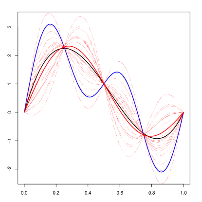
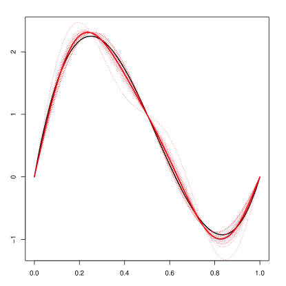
Figure 1: Heat equation with unknown diffusivity parameter: True function (black), projection estimator (blue), posterior mean (red, solid) and 20 draws from the posterior distribution (red, dotted) with $\varepsilon=\delta=10^{-6}$ (left) and $10^{-8}$ (right).

Figure 1 shows the typical posterior mean and 20 draws from the posterior distribution in a simulation using $\varepsilon=\delta=10^{-6}$ and $10^{-8}$. In both cases the projection level is chosen as $J=4\simeq\sqrt{-\log(\varepsilon)}$. Especially for the smaller noise level, the common intersections of all sampled functions are conspicuous. They reflect a quite low variance of the posterior distribution in the first coefficients compared to a relatively large variance already for $f_{4}$ due to the severe ill-posedness, cf. (6.4).

As a reference estimator the Galerkin projector $\widehat{f}_{J}$ from (3.6) is plotted, too. We see that for $\varepsilon=10^{-6}$ the posterior mean is much closer to the true function indicating an efficiency gain of the Bayesian procedure compared to the projection estimator. For $\varepsilon=10^{-8}$ both estimators coincide almost perfectly. As shown by the theory, the figure illustrates that the posterior distribution concentrates around the truth for smaller noise levels. Monte Carlo simulations based on 500 iterations yield a root mean integrated squared error (RMISE) 0.3353 and 0.0512 for $\varepsilon=10^{-6}$ and $\varepsilon=10^{-8}$, respectively. For the posterior mean of $\vartheta$ we observe a root mean squared error of approximately $1.0\cdot 10^{-6}$ and $9.7\cdot 10^{-9}$, respectively. Additionally, Table 1 reports the RMISE for several different combinations of the noise levels $\varepsilon$ and $\delta$.

$\delta$ \  $\varepsilon$	$10^{-4}$	$10^{-6}$	$10^{-8}$
$10^{-4}$	0.5728	0.3173	0.5656
$10^{-6}$	0.5515	0.3353	0.0545
$10^{-8}$	0.5548	0.3269	0.0512

Table 1: RMISE for different values of $\varepsilon$ and $\delta$.

6.2 Deconvolution with unknown kernel

Another example is the deconvolution problem occurring for instance in image processing, cf. Johnstone et al., [19]. The aim is to recover some unknown 1-periodic function $f$ from the observations

$$Y=K_{\vartheta}f+\varepsilon Z\quad\text{with}\quad K_{\vartheta}f:=g_{\vartheta}\ast f:=\int_{0}^{1}f(\cdot-x)g_{\vartheta}(x)\mathrm{d}x$$

where $g_{\vartheta}\in L^{2}_{per}$ is some $1$-periodic convolution kernel (more general it might be a signed measure). Since the convolution operator $K_{\vartheta}$ is smoothing, the inverse problem is ill-posed. If the kernel $g_{\vartheta}$ is unknown, the problem is called blind deconvolution occurring in many applications [4, 20, 32]. In a density estimation setting this problem as already been intensively investigated, cf. [10, 17, 18, 26] among others. However, the Bayesian perspective on this problem seem not thoroughly studied.

We consider the trigonometric basis

$$\varphi_{0}=1,\quad\varphi_{j,0}=\sqrt{2}\sin(2\pi j\cdot),\qquad\varphi_{j,1}=\sqrt{2}\cos(2\pi j\cdot),\qquad j\in\mathbb{N},$$

with the corresponding approximation spaces $V_{J}=\operatorname{span}(\varphi_{j,l}:j\leqslant J,l\in\{0,1\})$. Assuming $g_{\vartheta}$ is symmetric, we have $\langle g_{\vartheta},\varphi_{j,0}\rangle=0$ and

$$K_{\vartheta}\varphi_{0}=\langle g_{\vartheta},\varphi_{0}\rangle\varphi_{0},\quad K_{\vartheta}\varphi_{j,l} =\sum_{m}\langle g_{\vartheta},\varphi_{m,1}\rangle(\varphi_{j,l}\ast\varphi_{m,1})=\frac{1}{\sqrt{2}}\langle g_{\vartheta},\varphi_{j,1}\rangle\varphi_{j,l},\quad j\in\mathbb{N},l\in\{0,1\}$$

by the angle sum identities (for non-symmetric kernels $K_{\vartheta}$ could be diagonolised by the complex valued Fourier basis). We thus obtain the singular value decomposition $K_{\vartheta}f=\sum_{k}\rho_{\vartheta,k}f_{k}\varphi_{k}$, again in muli-index notation $k=(j,l),j\in\mathbb{N},l\in\{0,1\}$, where $\rho_{\vartheta,k}=\langle g_{\vartheta},\varphi_{|k|,1}\rangle/\sqrt{2}$ and $f_{k}=\langle f,\varphi_{k}\rangle$. Depending on the regularity of $g$ and thus the decay of $\langle g_{\vartheta},\varphi_{j,1}\rangle$ the problem is mildly or severely ill-posed.

If the convolution kernel is fully unknown, we parametrise $g_{\vartheta}=\vartheta$ by all (symmetric) 1-periodic kernels $\vartheta$. Due to the SVD, we then can identify $g_{\vartheta}$ with the singular values, that is, we set $\vartheta=(\rho_{\vartheta,k})_{k}$. The sample $T$ can be understood as training data, where the convolution experiment is applied to all basis functions $f\in\{\varphi_{j,l}\}$. In this scenario we obtain $\varepsilon=\delta$.

In our simulation $\vartheta_{0}$ is given by the periodic Laplace kernel $g_{\vartheta_{0}}(x)=\frac{1}{C_{h}}e^{-|x|/h}\mathbbm{1}_{[-1/2,1/2]}(x)$ with normalisation constant $C_{h}=2h(1+e^{-1/(2h)})$ and fixed bandwidth $h=0.1$. Hence, we have for $k\in\mathbb{N}\times\{0,1\}$

$$\rho_{\vartheta_{0},0}=1,\qquad\rho_{\vartheta_{0},k}=\frac{2h^{-1}}{C_{h}(4\pi^{2}|k|^{2}+h^{-2})}\big{(}1-e^{-1/(2h)}\cos(\pi|k|)+e^{-1/(2h)}2\pi|k|h\sin(\pi|k|)\big{)}$$

In particular, we have two degree of illposedness. We moreover use $f_{0}$ from (6.3).

To implement the empirical Bayes procedure with the trigonometric basis and corresponding approximation spaces $V_{j}=\operatorname{span}(\varphi_{k}:|k|\leqslant j)$, we need to replace $2^{j}$ by $2j$ as mentioned in Remark 8. Choosing some $b>1$ and setting $\mathcal{J}_{\varepsilon}=\Big{\lfloor}\frac{\log\varepsilon^{-1}}{(s_{0}+t+d/2)\log b}\Big{\rfloor}$ for some lower bound $s_{0}\leqslant s$, the selection rule then reads as

$$\widehat{J}:=\min\big{\{}j\in\{1,b,b^{2},\dots,b^{\mathcal{J}_{\varepsilon}}\}:\|\widehat{f}_{i}-\widehat{f}_{j}\|\leqslant\Delta\varepsilon(\log\varepsilon^{-1})^{2}i^{3/2}\forall i>j\big{\}}.$$

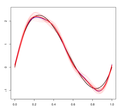
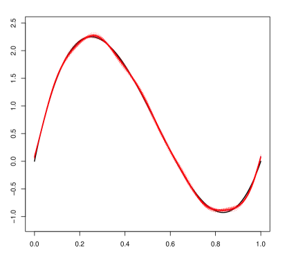
Figure 2: Adaptive deconvolution for the Laplace kernel with $\varepsilon=\delta=10^{-2}$ (left) and $\varepsilon=\delta=10^{-3}$ (right): True function (black), projection estimator (blue), posterior mean (red, solid) and 20 draws from the posterior distribution (red, dotted).

Using the again Gaussian product priors for $f$ and $\vartheta$, the posterior distribution can be similarly approximated as described in Section 6.1. However, the nuisance parameter $\vartheta$ is now infinite dimensional. Here, we can profit from the truncated product structure of the prior which implies that the posterior distribution only depends on the $\widehat{J}$-dimensional projection $P_{\widehat{J}}\vartheta$ (note that Assumption 1 is satisfied with $m=0$). More precisely, we only have to draw from the posterior given by

$$\Pi(B|Y,T)=\frac{1}{C}\int_{B}\exp\Big{(}\frac{1}{\varepsilon^{2}}\langle P_{\widehat{J}}K_{\vartheta}f,Y\rangle-\frac{1}{2\varepsilon^{2}}\|P_{\widehat{J}}K_{\vartheta}f\|^{2}+\frac{1}{\delta^{2}}\langle P_{\widehat{J}}\vartheta,T\rangle-\frac{1}{2\delta^{2}}\|P_{\widehat{J}}\vartheta\|^{2}\Big{)}\mathrm{d}\Pi(f,\vartheta),$$

with normalisation constant $C>0$ and for all Borel sets $B\subseteq L^{2}\times P_{\widehat{J}}\Theta$, cf. proof of Theorem 5. Therefore, a Gibbs sampler can be used to draw successively the coordinates of $P_{\widehat{J}}\vartheta$ with a Metropolis-Hastings algorithm and iterate as above with draws of $f$. This simulation approach is not restricted to this particular example, but applies generally. Note that in the specific deconvolution setting, the map $\vartheta\mapsto K_{\vartheta}f$ is linear for fixed $f$, such that $\vartheta|f,Y,T$ can be directly sampled from a Gaussian distribution.

For $\varepsilon=\delta=10^{-2}$ and $\varepsilon=\delta=10^{-3}$ a typical trajectory of the posterior mean and 20 draws from the posterior are presented in Figure 2 where the Lepski rule has chosen $J=3$ (i.e. 7 basis functions) and $J=5$ (11 basis functions), respectively. For the larger noise level, the posterior mean slightly improves the Galerkin projector, while for the smaller noise level both estimators basically coincide. We see a much better concentration of the posterior distribution than in the severely ill-posed case discussed previously. In a Monte Carlo simulation for $\varepsilon=\delta=10^{-2}$ based on 500 iterations in this setting the posterior mean for $f$ achieved a RMISE of 0.1142 which is approximately $8.6\%$ of $\|f_{0}\|$. The Lepski method has chosen $J\in\{2,3\}$ with relative frequency $0.97$. For $\varepsilon=\delta=10^{-2}$ the simulation yields a RMISE of 0.0174, which is $1.3\%$ of $\|f_{0}\|$, and projections levels $J$ in $\{4,5\}$ in $0.82\%$ of the Monte Carlo iterations.

7 Proofs

We first study some smoothing properties of the operator $K_{\vartheta}$.

Lemma 14.

Under Assumption 4 we have $\|K_{\vartheta,j}^{-1}\|_{V_{j}\to V_{j}}\leqslant Q\sigma_{j}^{-1}$ for all $\vartheta\in\Theta$.

Proof.

For $g\in V_{j}$ the function $h=K_{\vartheta,j}^{-1}g\in V_{j}$ is given by the unique solution to the linear system

$$\langle K_{\vartheta}h,v\rangle=\langle g,v\rangle,\qquad\text{for all }v\in V_{j}.$$

Assumption 4 then yields

$$\sigma_{j}\|h\|^{2} =\sigma_{j}\sum_{|k|\leqslant j}\langle h,\varphi_{k}\rangle^{2}\leqslant\sum_{|k|\leqslant j}\sigma_{|k|}\langle h,\varphi_{k}\rangle^{2}$$

$$=Q\langle K_{\vartheta}h,h\rangle\leqslant Q\|h\|\sup_{v\in V_{j}:\|v\|\leqslant 1}\langle K_{\vartheta}h,v\rangle=Q\|h\|\sup_{v\in V_{j}:\|v\|\leqslant 1}\langle g,v\rangle=Q\|h\|\|g\|.$$

Therefore, $\sigma_{j}\|K_{\vartheta,j}^{-1}g\|\leqslant Q\|g\|$ holds true for all $g\in V_{j}$. ∎

Remark 15.

As soon as $(\sigma_{j})$ decays at least geometrically, Assumptions 1 and 4 also yield $\|K_{\vartheta}f\|^{2}\lesssim\sum_{k}\sigma_{|k|}^{2}\langle f,\varphi_{k}\rangle^{2}$. Indeed, we have for any $f\in L^{2}$ such that the right-hand side is finite:

$$\|K_{\vartheta}f\|^{2} =\sum_{k}|\langle K_{\vartheta}P_{|k|+m}f,\varphi_{k}\rangle|^{2}\leqslant\sum_{k}\|K_{\vartheta}^{1/2}P_{|k|+m}f\|^{2}\|K_{\vartheta}^{1/2}\varphi_{k}\|^{2}$$

$$\lesssim\sum_{k}\sum_{|l|\leqslant|k|+m}\sigma_{|k|}\sigma_{|l|}\langle f,\varphi_{l}\rangle^{2}=\sum_{l}\Big{(}\sum_{|k|\geqslant(|l|-m)\vee 0}\sigma_{|k|}\Big{)}\sigma_{|l|}\langle f,\varphi_{l}\rangle^{2}\lesssim\sum_{l}\sigma^{2}_{|l|}\langle f,\varphi_{l}\rangle^{2}.$$

7.1 Proof of Proposition 6

To simplify the notation, we abbreviate $\mathbb{P}=\mathbb{P}_{f,\vartheta}$ in the sequel and define the operator $\Delta_{T,j}:=K_{T,j}-K_{\vartheta,j}$. Set for $\gamma\in(0,1-Q/\tau)$

$$\Omega_{T,j}:=\{\|K_{\vartheta,j}^{-1}\Delta_{T,j}\|_{V_{j}\to V_{j}}\leqslant\gamma\}.$$

Lemma 14 yields

$$\mathbb{P}\big{(}\Omega_{T,j}^{c}\big{)}\leqslant\mathbb{P}\big{(}\|K_{\vartheta,j}^{-1}\|_{V_{j}\to V_{j}}\|\Delta_{T,j}\|_{V_{j}\to V_{j}}>\gamma\big{)}\leqslant\mathbb{P}\big{(}\|\Delta_{T,j}\|_{V_{j}\to V_{j}}>\gamma\sigma_{j}/Q\big{)}.$$

Under Assumption 2 we have due to the condition $\delta\sigma_{j}^{-1}(\kappa+\sqrt{d_{j}})\leqslant\gamma/(CQL)$

$$\mathbb{P}\big{(}\Omega_{T,j}^{c}\big{)}\leqslant \mathbb{P}\big{(}\|\Delta_{T,j}\|_{V_{j}\to V_{j}}>\gamma\sigma_{j}/Q\big{)}$$

$$\leqslant \mathbb{P}\Big{(}\|P_{j}W\|_{j}\geqslant\frac{\gamma\sigma_{j}}{QL}\Big{)}\leqslant\mathbb{P}\big{(}\|P_{j}W\|_{V_{j}\to V_{j}}>C\delta(\kappa+\sqrt{d_{j}})\big{)}\leqslant e^{-c\kappa^{2}}.$$

We thus may restrict on $\Omega_{T,j}$ on which the operator $K_{T,j}=K_{\vartheta,j}(\operatorname{Id}-K_{\vartheta,j}^{-1}\Delta_{T,j})$ is invertible satisfying

$$\|K_{T,j}^{-1}\|_{V_{j}\to V_{j}}\leqslant\|(\operatorname{Id}-K_{\vartheta,j}^{-1}\Delta_{T,j})^{-1}\|_{V_{j}\to V_{j}}\|K_{\vartheta,j}^{-1}\|_{V_{j}\to V_{j}}\leqslant\frac{1}{1-\gamma}\|K_{\vartheta,j}^{-1}\|_{V_{j}\to V_{j}}\leqslant\frac{Q}{(1-\gamma)\sigma_{j}}$$

where we used Lemma 14 in the last step. Hence, for $\gamma\leqslant 1-Q/\tau$ we have $\Omega_{T,j}\subseteq\{\|K_{T,j}^{-1}\|_{V_{j}\to V_{j}}\leqslant\tau\sigma_{j}^{-1}\}$. Therefore, we can decompose on $\Omega_{T,j}$

$$\|\widehat{f}_{j}-f\|^{2} =\|P_{j}f-f\|^{2}+\|\widehat{f}_{j}-P_{j}f\|^{2}$$

$$\leqslant\|P_{j}f-f\|^{2}+\|K_{T,j}^{-1}P_{j}Y-P_{j}f\|^{2}.$$ (7.1)

The first term is the usual bias. For the second term in (7.1) we write on $\Omega_{T,j}$

$$K_{T,j}^{-1}P_{j}Y-P_{j}f =\big{(}(\operatorname{Id}-K_{\vartheta,j}^{-1}\Delta_{T,j})^{-1}-\operatorname{Id}\big{)}P_{j}f+\varepsilon(\operatorname{Id}-K_{\vartheta,j}^{-1}\Delta_{T,j})^{-1}K_{\vartheta,j}^{-1}P_{j}Z$$

$$=(\operatorname{Id}-K_{\vartheta,j}^{-1}\Delta_{T,j})^{-1}K_{\vartheta,j}^{-1}\Delta_{T,j}P_{j}f+\varepsilon(\operatorname{Id}-K_{\vartheta,j}^{-1}\Delta_{T,j})^{-1}K_{\vartheta,j}^{-1}P_{j}Z.$$

Since $\|(\operatorname{Id}-K_{\vartheta,j}^{-1}\Delta_{T,j})^{-1}\|_{V_{j}\to V_{j}}\leqslant 1/(1-\gamma)$ on $\Omega_{T,j}$, we obtain

$$\|K_{T,j}^{-1}P_{j}Y-P_{j}f\| \leqslant\frac{1}{1-\gamma}\|K_{\vartheta,j}^{-1}\|_{V_{j}\to V_{j}}\|\Delta_{T,j}\|_{V_{j}\to V_{j}}\|P_{j}f\|+\frac{\varepsilon}{1-\gamma}\|K_{\vartheta,j}^{-1}\|_{V_{j}\to V_{j}}\|P_{j}Z\|$$

$$\leqslant\frac{Q}{(1-\gamma)\sigma_{j}}\big{(}\|f\|\|\Delta_{T,j}\|_{V_{j}\to V_{j}}+\varepsilon\|P_{j}Z\|\big{)}.$$ (7.2)

To deduce a concentration inequality for $\|P_{j}Z\|$, we proceed as proposed in [13]: For a countable dense subset $B$ of the unit ball in $L^{2}$, we have $\|P_{j}Z\|=\sup_{f\in B}\|P_{j}Z(f)\|$. The Borell-Sudakov-Tsirelson inequality [14, Thm. 2.5.8] yields for any $\kappa>0$

$$\mathbb{P}(\|P_{j}Z\|\geqslant\kappa+\mathbb{E}[\|P_{j}Z\|]) \leqslant\mathbb{P}\Big{(}\sup_{f\in B}\|P_{j}Z(f)\|-\mathbb{E}\Big{[}\sup_{f\in B}\|P_{j}Z(f)\|\Big{]}\geqslant\kappa\Big{)}\leqslant 2^{-\kappa^{2}/(2\sigma^{2})}$$

with $\sigma^{2}=\sup_{f\in B}\operatorname{Var}(P_{j}Z(f))\leqslant\|f\|^{2}\leqslant 1$. Since

$$\mathbb{E}[\|P_{j}Z\|]\leqslant\mathbb{E}[\|P_{j}Z\|^{2}]^{1/2}=\Big{(}\sum_{|k|\leqslant j}\mathbb{E}[Z_{k}^{2}]\Big{)}^{1/2}=d_{j}^{1/2}$$

and $d_{j}\lesssim\varepsilon^{-2}\kappa^{2}$, we find for some constant $C>0$

$$\mathbb{P}\big{(}\varepsilon\|P_{j}Z\|\geqslant C\kappa\big{)}\leqslant\mathbb{P}\big{(}\varepsilon\|P_{j}Z\|\geqslant\kappa+\varepsilon d_{j}^{1/2}\big{)}\leqslant e^{-\kappa^{2}/(2\varepsilon^{2})}.$$

Under Assumption 2 and due to $d_{j}\lesssim\delta^{-2}\kappa^{2}$, we analogously obtain

$$\mathbb{P}\big{(}\|\Delta_{T,j}\|_{V_{j}\to V_{j}}\geqslant C\kappa\big{)}\leqslant e^{-\kappa^{2}/(2\delta^{2})}.$$

In combination with (7.2), the asserted concentration inequality is proven.∎

7.2 Proof of Theorem 5

We proof the theorem in two steps.

Step 1: We construct tests $\Psi_{n}=\Psi_{n}(Y,T)$ such that

$$\mathbb{E}_{f_{0},\vartheta_{0}}[\Psi_{n}]\to 0\qquad\text{and}\sup_{f\in\mathcal{F}_{n},\vartheta\in\Theta:\|f-f_{0}\|\geqslant D\xi_{n}}\mathbb{E}_{f,\vartheta}[1-\Psi_{n}]\leqslant 3e^{-(C_{1}+4)\kappa_{n}^{2}/(\varepsilon_{n}\vee\delta_{n})^{2}}.$$ (7.3)

Based on the estimator $\widehat{f}_{j_{n}}$ from (3.6), we set

$$\Psi_{n}:=\mathbbm{1}_{\{\|\widehat{f}_{j_{n}}-f_{0}\|\geqslant D_{1}\xi_{n}\}}$$

for $D_{1}=2Cc_{2}\sqrt{C_{1}+4}R+2C_{0}\xi_{n}$ with the constant $C$ from Proposition 6. Due to Proposition 6 and $\kappa_{n}/\sigma_{j_{n}}\leqslant c_{2}\xi_{n}$, we then have

$$\mathbb{E}_{f_{0},\vartheta_{0}}[\Psi_{n}] =\mathbb{P}_{f_{0},\vartheta_{0}}\Big{(}\|\widehat{f}_{j_{n}}-f_{0}\|\geqslant 2C\sigma_{j_{n}}^{-1}\sqrt{C_{1}+4}\kappa_{n}\|f_{0}\|+2C_{0}\xi_{n}\Big{)}$$

$$\leqslant\mathbb{P}_{f_{0},\vartheta_{0}}\big{(}\|\widehat{f}_{j_{n}}-f_{0}\|\geqslant C\sigma_{j_{n}}^{-1}\sqrt{C_{1}+4}\kappa_{n}\|f_{0}\|+\|f_{0}-P_{j_{n}}f_{0}\|\big{)}\leqslant 3e^{-(C_{1}+4)\kappa_{n}^{2}/(\varepsilon_{n}\vee\delta_{n})^{2}}$$

converging to 0.

On the alternative we set $D=D_{2}(1+R)$ for $D_{2}=2\max(C_{0}+D_{1},C\sqrt{C_{1}+4}/c_{2})$. For any $\vartheta\in\Theta$ and any $f\in\mathcal{F}_{n}$ with $\|f-f_{0}\|\geqslant D_{2}(1+R)\xi_{n}$ we have $(2-D_{2}\xi_{n})\|f-f_{0}\|\geqslant D_{2}(1+R)\xi_{n}$ for sufficiently small $\xi_{n}\downarrow 0$. Therefore,

$$\|f-f_{0}\|\geqslant \frac{D_{2}}{2}(1+R+\|f-f_{0}\|)\xi_{n}\geqslant\frac{D_{2}}{2}\big{(}1+\|f_{0}\|+\|f-f_{0}\|\big{)}\xi_{n}$$

$$\geqslant \frac{D_{2}}{2}(1+\|f\|)\xi_{n}\geqslant C\sigma_{j_{n}}^{-1}\sqrt{C_{1}+4}\kappa_{n}\|f\|+(C_{0}+D_{1})\xi_{n},$$ (7.4)

where the last inequality holds by the choice of $D_{2}$. We obtain

$$\mathbb{E}_{f,\vartheta}[1-\Psi_{n}] =\mathbb{P}_{f,\vartheta}\big{(}\|\widehat{f}_{j_{n}}-f_{0}\|<D_{1}\xi_{n}\big{)}$$

$$\leqslant\mathbb{P}_{f,\vartheta}\big{(}\|\widehat{f}_{j_{n}}-f\|>\|f-f_{0}\|-D_{1}\xi_{n}\big{)}$$

$$\leqslant\mathbb{P}_{f,\vartheta}\big{(}\|\widehat{f}_{j_{n}}-f\|>C\sigma_{j_{n}}^{-1}\sqrt{C_{1}+4}\kappa_{n}\|f\|+C_{0}\xi_{n}\big{)}.$$

Proposition 6 yields again $\mathbb{E}_{f,\vartheta}[1-\Psi_{n}]\leqslant 3e^{-(C_{1}+4)\kappa_{n}^{2}/(\varepsilon_{n}\vee\delta_{n})^{2}}$.

Step 2: Since $\mathbb{E}_{f_{0},\vartheta_{0}}[\Psi_{n}]\to 0$, it suffices to prove that

$$\Pi_{n}\big{(}f \in V_{j_{n}}:\|f-f_{0}\|>D\xi_{n}|Y,T\big{)}(1-\Psi_{n})$$

$$= \frac{\int_{f\in V_{j_{n}}:\|f-f_{0}\|>D\xi_{n},\vartheta\in\Theta}p_{f,\vartheta}(Z,W)\mathrm{d}\Pi_{n}(f,\vartheta)(1-\Psi_{n})}{\int_{f\in\mathcal{F},\vartheta\in\Theta}p_{f,\vartheta}(Z,W)\mathrm{d}\Pi_{n}(f,\vartheta)}\to 0\quad\text{in }P_{f_{0},\vartheta_{0}}\text{-probability.}$$

Due to Assumption 1, we have $K_{\vartheta}P_{j_{n}}=P_{j_{n}+m}K_{\vartheta}P_{j_{n}}=K_{\vartheta,j_{n}+m}P_{j_{n}}$. Hence, restricted on $f\in V_{j_{n}}$, we obtain

$$p_{f,\vartheta}(z,w) =\exp\Big{(}\frac{1}{\varepsilon}\langle K_{\vartheta,j_{n}+m}f-K_{\vartheta_{0}}f_{0},z\rangle-\frac{1}{2\varepsilon^{2}}\|K_{\vartheta,j_{n}+m}f-K_{\vartheta_{0}}f_{0}\|^{2}$$

$$\hskip 50.00008pt+\frac{1}{\delta}\langle\vartheta-\vartheta_{0},w\rangle-\frac{1}{2\delta^{2}}\|\vartheta-\vartheta_{0}\|^{2}\Big{)}$$

$$=\exp\Big{(}\frac{1}{\varepsilon}\langle K_{\vartheta,j_{n}+m}f-K_{\vartheta_{0}}f_{0},z\rangle-\frac{1}{2\varepsilon^{2}}\|K_{\vartheta,j_{n}+m}f-P_{j_{n}+m}K_{\vartheta_{0}}f_{0}\|^{2}$$

$$\hskip 50.00008pt-\frac{1}{2\varepsilon^{2}}\|(\operatorname{Id}-P_{j_{n}+m})K_{\vartheta_{0}}f_{0}\|^{2}+\frac{1}{\delta}\langle\vartheta-\vartheta_{0},w\rangle-\frac{1}{2\delta^{2}}\|\vartheta-\vartheta_{0}\|^{2}\Big{)}.$$

Since we assume that $K_{\vartheta,j_{n}+m}$ depends only on $P_{j_{n}+m}\vartheta=(\vartheta_{1},\dots,\vartheta_{l_{j_{n}+m}})$ and $\Pi$ is a product prior in $(\vartheta_{k})$, we may rewrite

$$\Pi_{n}\big{(}f \in V_{j_{n}}:\|f-f_{0}\|>D\xi_{n}|Y,T\big{)}(1-\Psi_{n})$$ (7.5)

$$\qquad\leqslant\frac{\int_{f\in\mathcal{F}\cap V_{j_{n}}:\|f-f_{0}\|>D\xi_{n},\vartheta\in\Theta}p_{f,\vartheta}^{(j_{n})}(Z,W)\mathrm{d}\Pi_{n}(f,\vartheta)(1-\Psi_{n})}{\int_{f\in\mathcal{F}\cap V_{j_{n}},\vartheta\in\Theta}p_{f,\vartheta}^{(j_{n})}(Z,W)\mathrm{d}\Pi_{n}(f,\vartheta)}$$

with

$$p_{f,\vartheta}^{(j_{n})}(z,w) =\exp\Big{(}\frac{1}{\varepsilon}\langle P_{j_{n}+m}(K_{\vartheta}f-K_{\vartheta_{0}}f_{0}),z\rangle-\frac{1}{2\varepsilon^{2}}\|P_{j_{n}+m}(K_{\vartheta}f-K_{\vartheta_{0}}f_{0})\|^{2}$$

$$\hskip 50.00008pt+\frac{1}{\delta}\langle P_{j_{n}+m}(\vartheta-\vartheta_{0}),w\rangle-\frac{1}{2\delta^{2}}\|P_{j_{n}+m}(\vartheta-\vartheta_{0})\|^{2}\Big{)}.$$

We can proceed as in the proof of the Theorems 7.3.1 and 7.3.5, respectively, in [14]. First we need a lower bound for the denominator in (7.5). Defining the event

$$B_{n}:=\Big{\{}(f,\vartheta)\in V_{j_{n}}\times\Theta:\frac{\|P_{j_{n}+m}(K_{\vartheta}f-K_{\vartheta_{0}}f_{0})\|^{2}}{\varepsilon_{n}^{2}}+\frac{\|P_{j_{n}+m}(\vartheta-\vartheta_{0})\|^{2}}{\delta_{n}^{2}}\leqslant\frac{\kappa_{n}^{2}}{(\varepsilon_{n}\vee\delta_{n})^{2}}\Big{\}},$$

we obtain

$$\mathbb{P}_{f_{0},\vartheta_{0}}\Big{(}\int_{f\in\mathcal{F}\cap V_{j_{n}},\vartheta\in\Theta}p_{f,\vartheta}^{(j_{n})}(Z,W)\mathrm{d}\Pi_{n}(f,\vartheta)\geqslant e^{-(C_{1}+2)\kappa_{n}^{2}/(\varepsilon_{n}\vee\delta_{n})^{2}}\Big{)}$$

$$\qquad\geqslant\mathbb{P}_{f_{0},\vartheta_{0}}\Big{(}\int_{B_{n}}p_{f,\vartheta}^{(j_{n})}(Z,W)\frac{\mathrm{d}\Pi_{n}(f,\vartheta)}{\Pi_{n}(B_{n})}\geqslant e^{-2\kappa_{n}^{2}/(\varepsilon_{n}\vee\delta_{n})^{2}}\Big{)}\geqslant 1-\frac{(\varepsilon_{n}\vee\delta_{n})^{2}}{\kappa_{n}^{2}},$$

where the first inequality is due to the small ball probability (3.3) and the second inequality follows along the lines of Lemma 7.3.4 in [14]. Using this bound for the denominator together with Markov’s inequality and Fubini’s theorem, the probability that (7.5) is larger than some $r>0$ is bounded by

$$\mathbb{P}_{f_{0},\vartheta_{0}}\Big{(}\Pi_{n}(f\in V_{j_{n}}:\|f-f_{0}\|>D\xi_{n}|Y,T)(1-\Psi_{n})\geqslant r\Big{)}$$

$$\qquad\leqslant\mathbb{P}_{f_{0},\vartheta_{0}}\Big{(}e^{(C_{1}+2)\kappa_{n}^{2}/(\varepsilon_{n}\vee\delta_{n})^{2}}(1-\Psi_{n})\int_{f,\vartheta:\|f-f_{0}\|>D\xi_{n}}p_{f,\vartheta}^{(j_{n})}(Z,W)\mathrm{d}\Pi_{n}(f,\vartheta)\geqslant r\Big{)}+\frac{(\varepsilon_{n}\vee\delta_{n})^{2}}{\kappa_{n}^{2}}$$

$$\qquad\leqslant\frac{e^{(C_{1}+2)\kappa_{n}^{2}/(\varepsilon_{n}\vee\delta_{n})^{2}}}{r}\mathbb{E}_{f_{0},\vartheta_{0}}\Big{[}(1-\Psi_{n})\int_{f,\vartheta:\|f-f_{0}\|>D\xi_{n}}p_{f,\vartheta}^{(j_{n})}(Z,W)\mathrm{d}\Pi_{n}(f,\vartheta)\Big{]}+\frac{(\varepsilon_{n}\vee\delta_{n})^{2}}{\kappa_{n}^{2}}$$

$$\qquad\leqslant\frac{e^{(C_{1}+2)\kappa_{n}^{2}/(\varepsilon_{n}\vee\delta_{n})^{2}}}{r}\int_{f,\vartheta:\|f-f_{0}\|>D\xi_{n}}\mathbb{E}_{f_{0},\vartheta_{0}}\Big{[}(1-\Psi_{n})p_{f,\vartheta}^{(j_{n})}(Z,W)\Big{]}\mathrm{d}\Pi_{n}(f,\vartheta)+\frac{(\varepsilon_{n}\vee\delta_{n})^{2}}{\kappa_{n}^{2}}.$$

Note that $p_{f,\vartheta}^{(j_{n})}$ corresponds to the density of the law of $(Y^{\prime},T^{\prime})$ where

$$Y^{\prime}=P_{j_{n}+m}K_{\vartheta}f+(\operatorname{Id}-P_{j_{n}+m})K_{\vartheta_{0}}f_{0}+\varepsilon Z\quad\text{and}\quad T^{\prime}=P_{j_{n}+m}\vartheta+(\operatorname{Id}-P_{j_{n}+m})\vartheta_{0}+\delta W$$

with respect to $\mathbb{P}_{\vartheta_{0},f_{0}}^{Y}\otimes\mathbb{P}_{\vartheta_{0}}^{T}$ and we have $\Psi_{n}(Y,T)=\Psi_{n}(Y^{\prime},T^{\prime})$ by construction. Therefore, we can apply Step 1 to bound the previous display and conclude

$$\mathbb{P}_{f_{0},\vartheta_{0}}\Big{(}\Pi_{n}(f\in V_{j_{n}}:\|f-f_{0}\|>D\xi_{n}|Y,T)\geqslant r\Big{)}\lesssim\frac{1}{r}e^{-2\kappa_{n}^{2}/(\varepsilon_{n}\vee\delta_{n})^{2}}+\frac{(\varepsilon_{n}\vee\delta_{n})^{2}}{\kappa_{n}^{2}}+\mathbb{E}_{f_{0},\vartheta_{0}}[\Psi_{n}].$$ (7.6)

It remains to note that for any $r>0$ the right-hand side converges to zero as $n\to\infty$ . ∎

7.3 Proof of Theorem 10

For the sake of brevity we omit the subscript $n$ in the proof. $c_{1},c_{2},\dots$ will denote positive, universal constants. We will choose $\kappa,\xi$ and $j=J$ according to

$$\xi\simeq\Big{(}(\varepsilon\vee\delta)\log\frac{1}{\varepsilon\vee\delta}\Big{)}^{2s/(2s+2t+d)},\kappa\simeq\Big{(}(\varepsilon\vee\delta)\log\frac{1}{\varepsilon\vee\delta}\Big{)}^{2(s+t)/(2s+2t+d)},2^{j}=\kappa^{-1/(s+t)}.$$ (7.7)

It is not difficult to see that these choices satisfy the requirements of Theorem 5 and $\|f_{0}-P_{j}f_{0}\|\lesssim\xi$ holds by (4.2). Moreover, the support of $\Pi_{f}$ lies in $V_{j}$ such that (3.2) is trivially satisfied for $\mathcal{F}_{n}=\{f:\|f-P_{j}f\|\leqslant C_{0}\xi\}$. It only remains to verify the small ball probability (3.3).

Owing to $P_{j}K_{\vartheta}=P_{j}K_{\vartheta}P_{j+m}=P_{j}K_{\vartheta,j+m}$, (4.2) and $\|K_{\vartheta}f\|\lesssim\|f\|_{H^{-t}}$, we can estimate for any $f\in V_{j}$

$$\|P_{j+m}(K_{\vartheta}f-K_{\vartheta_{0}}f_{0})\|\leqslant \|P_{j+m}(K_{\vartheta}-K_{\vartheta_{0}})f_{0}\|+\|P_{j+m}K_{\vartheta,j+2m}(f-f_{0})\|$$

$$\leqslant \|(K_{\vartheta,j+2m}-K_{\vartheta_{0},j+2m})f_{0}\|+\|K_{\vartheta}P_{j+2m}(f-f_{0})\|$$

$$\leqslant R\|K_{\vartheta,j+2m}-K_{\vartheta_{0},j+2m}\|_{V_{j+2m}\to V_{j+2m}}+\|f-P_{j+2m}f_{0}\|_{H^{-t}}$$

$$\leqslant R\|K_{\vartheta,j+2m}-K_{\vartheta_{0},j+2m}\|_{V_{j+2m}\to V_{j+2m}}+\|f-P_{j}f_{0}\|_{H^{-t}}$$

$$\quad+\|P_{j+2m}(\operatorname{Id}-P_{j})f_{0}\|_{H^{-t}}.$$

The last term is bounded by $\|(\operatorname{Id}-P_{j})f_{0}\|_{H^{-t}}\lesssim 2^{-j(s+t)}\|f_{0}\|_{H^{s}}$ being of the order $\mathcal{O}(\kappa\varepsilon/(\varepsilon\vee\delta))$ due to $\varepsilon\gtrsim\delta$ and the choice $j$ as in (7.7). We obtain

$$\Pi\big{(}f\in\mathcal{F}\cap V_{j},\vartheta\in\Theta:\varepsilon^{-2}\|P_{j+m}(K_{\vartheta}f-K_{\vartheta_{0}}f_{0})\|^{2}+\delta^{-2}\|P_{j+m}(\vartheta-\vartheta_{0})\|^{2}\leqslant\kappa^{2}/(\varepsilon\vee\delta)^{2}\big{)}$$

$$\quad\geqslant\Pi\Big{(}f\in\mathcal{F}\cap V_{j},\vartheta\in\Theta:\frac{1}{\varepsilon^{2}}\|f-P_{j}f_{0}\|_{H^{-t}}^{2}+\frac{R^{2}}{\varepsilon^{2}}\|K_{\vartheta,j+2m}-K_{\vartheta_{0},j+2m}\|_{V_{j+2m}\to V_{j+2m}}^{2}$$

$$\quad\qquad\qquad+\frac{1}{\delta^{2}}\|P_{j+m}(\vartheta-\vartheta_{0})\|^{2}\leqslant c_{1}\kappa^{2}/(\varepsilon\vee\delta)^{2}\Big{)}$$

$$\quad\geqslant\Pi_{f}\Big{(}f\in\mathcal{F}\cap V_{j}:\|f-P_{j}f_{0}\|_{H^{-t}}\leqslant\frac{c_{1}\varepsilon\kappa}{\sqrt{2}(\varepsilon\vee\delta)}\Big{)}$$

$$\quad\qquad\times\Pi_{\vartheta}\Big{(}\frac{1}{\varepsilon^{2}}\|K_{\vartheta,j+2m}-K_{\vartheta_{0},j+2m}\|_{V_{j+2m}\to V_{j+2m}}^{2}+\frac{1}{\delta^{2}}\|P_{j+m}(\vartheta-\vartheta_{0})\|^{2}\leqslant\frac{c_{1}\kappa^{2}}{2(\varepsilon\vee\delta)^{2}}\Big{)},$$ (7.8)

where the last line follows from independence of $f$ and $\vartheta$ under $\Pi$. The first term can be bounded using the product structure and the estimate (4.4). Setting $\widetilde{\kappa}=\frac{\varepsilon\kappa}{\varepsilon\vee\delta}$ and taking $\log\tau_{j}\lesssim j$ into account, we obtain

$$\Pi_{f}\Big{(}f\in\mathcal{F}\cap V_{j}:\|f-P_{j}f_{0}\|_{H^{-t}}\leqslant\frac{c_{1}\varepsilon\kappa}{\sqrt{2}(\varepsilon\vee\delta)}\Big{)}$$

$$\quad=\Pi_{f}\Big{(}f\in\mathcal{F}\cap V_{j}:\sum_{|k|\leqslant j}2^{-2t|k|}(f_{k}-f_{0,k})^{2}\leqslant\frac{c_{1}^{2}\widetilde{\kappa}^{2}}{2}\Big{)}$$

$$\quad\geqslant\prod_{|k|\leqslant j}\Pi_{f}\big{(}|f_{k}-f_{0,k}|\leqslant c_{2}\widetilde{\kappa}2^{(t-d/2)|k|}\big{)}$$

$$\quad\geqslant\exp\Big{(}c_{3}2^{jd}\log(2\Gamma)+c_{3}\sum_{|k|\leqslant j}\big{(}(2t-d)|k|-\log\tau_{|k|}+\log\widetilde{\kappa}\big{)}-2\gamma\sum_{|k|\leqslant j}\tau_{|k|}^{-2}\big{(}|f_{0,k}|^{2}+c_{3}\widetilde{\kappa}^{2}2^{(2t-d)|k|}\big{)}\Big{)}$$

$$\quad\geqslant\exp\Big{(}c_{4}2^{jd}(\log\widetilde{\kappa}-j)-2\gamma\max_{l\leqslant j}(2^{-2sl}\tau_{l}^{-2})\|f_{0}\|_{H^{s}}^{2}-c_{4}\widetilde{\kappa}^{2}\tau_{j}^{-2}2^{2tj}\Big{)}.$$

Since $\kappa\simeq 2^{-j(s+t)}$, we have $\log\widetilde{\kappa}^{-1}\lesssim j+\log\frac{\varepsilon\vee\delta}{\varepsilon}\lesssim j$. From the assumptions on $\tau_{j}$ we thus deduce

$$\Pi_{f}\Big{(}f\in\mathcal{F}\cap V_{j}:\|f-P_{j}f_{0}\|_{H^{-t}}\leqslant\frac{c_{1}\varepsilon\kappa}{\sqrt{2}(\varepsilon\vee\delta)}\Big{)}\geqslant e^{c_{5}2^{jd}(\log\widetilde{\kappa}-j)}\geqslant e^{-c_{6}j2^{jd}}.$$ (7.9)

By the the Lipschitz continuity $\|K_{\vartheta,j}-K_{\vartheta_{0},j}\|_{V_{j}\to V_{j}}^{2}\lesssim\|P_{j}(\vartheta-\vartheta_{0})\|^{2}$, the second term in (7.8) is bounded by

$$\Pi_{\vartheta}\Big{(}\Big{(}\frac{1}{\varepsilon^{2}}+\frac{1}{\delta^{2}}\Big{)}\|P_{j+2m}(\vartheta-\vartheta_{0})\|^{2}\leqslant\frac{c_{7}\kappa^{2}}{(\varepsilon\vee\delta)^{2}}\Big{)}\geqslant\Pi_{\vartheta}\Big{(}\|P_{j+m}(\vartheta-\vartheta_{0})\|\leqslant\frac{c_{7}(\varepsilon\wedge\delta)\kappa}{\varepsilon\vee\delta}\Big{)}.$$

Due to Assumption 9 and using again (4.4), we can estimate for $\bar{\kappa}=\frac{(\varepsilon\wedge\delta)\kappa}{\varepsilon\vee\delta}$:

$$\Pi_{\vartheta}\Big{(}\|P_{j+2m}(\vartheta-\vartheta_{0})\|\leqslant c_{7}\bar{\kappa}\Big{)}$$

$$\quad\geqslant\prod_{|k|\leqslant l_{j+m}}\Pi_{\vartheta}\big{(}|\vartheta_{k}-\vartheta_{k,0}|\leqslant c_{7}\bar{\kappa}/\sqrt{l_{j+2m}}\big{)}$$

$$\quad\geqslant\exp\Big{(}c_{8}l_{j+2m}\log(2\Gamma)+c_{8}l_{j+2m}\log\bar{\kappa}-\frac{c_{8}}{2}l_{j+2m}\log l_{j+2m}-\gamma\sum_{|k|\leqslant l_{j+2m}}\big{(}|\vartheta_{0,k}|+c_{7}\bar{\kappa}/\sqrt{l_{j+2m}}\big{)}^{2}\Big{)}$$

$$\quad\geqslant\exp\Big{(}c_{9}l_{j+2m}\log\bar{\kappa}-c_{9}l_{j+2m}\log l_{j+2m}-c_{9}\|\vartheta_{0}\|^{2}-c_{9}\bar{\kappa}^{2}\Big{)}$$

$$\quad\geqslant\exp\Big{(}-c_{10}l_{j+2m}\big{(}\log(\bar{\kappa}^{-1})+\log l_{j+2m}\big{)}\Big{)},$$

where we have used in the last step that $\bar{\kappa}\leqslant\kappa\to 0$. Because $\varepsilon^{\eta}\lesssim\delta$ implies $\log\bar{\kappa}^{-1}\lesssim j+\log\frac{\varepsilon\vee\delta}{\varepsilon\wedge\delta}\lesssim j$, we find in combination with $\log l_{j+2m}\lesssim j$ that

$$\Pi_{\vartheta}\Big{(}\|P_{j+m}(\vartheta-\vartheta_{0})\|\leqslant c_{7}\bar{\kappa}\Big{)}\geqslant e^{-c_{11}jl_{j+2m}}\gtrsim e^{-c_{12}j2^{jd}}.$$ (7.10)

Therefore, (3.3) follows from $j2^{jd}\leqslant\kappa^{2}(\varepsilon\vee\delta)^{-2}$, which is satisfied due to (7.7), in combination with (7.8), (7.9) and (7.10).∎

7.4 Proof of Theorem 12

The proof is similar to the previous one. The choices of $\kappa,\xi$ and $j$ given by

$$\xi\simeq\Big{(}\log\frac{1}{\varepsilon\vee\delta}\Big{)}^{-s/t},\qquad\kappa\simeq(\varepsilon\vee\delta)^{1/2},\qquad 2^{j}=\Big{(}-\frac{1}{2r}\log\big{(}\frac{\kappa\varepsilon}{\varepsilon\vee\delta}\big{)}\Big{)}^{1/t}$$ (7.11)

satisfy the conditions of Theorem 5. Especially, we have $\|f_{0}-P_{j}f_{0}\|\lesssim 2^{-js}\|f_{0}\|_{H_{s}}\lesssim\xi$ and $2^{J}=2^{j}(1+o(1))$ because of $\log\varepsilon\simeq\log\delta$. Since $\|K_{\vartheta}f\|^{2}\lesssim\sum_{k}e^{-2r2^{|k|t}}f_{k}^{2}$, we estimate for any $f\in\mathcal{F}\cap V_{j}$

$$\|P_{j+m}(K_{\vartheta}f-K_{\vartheta_{0}}f_{0})\|^{2}$$

$$\quad\leqslant 2\|(K_{\vartheta,j+2m}-K_{\vartheta_{0},j+2m})f_{0}\|^{2}+2\|K_{\vartheta}P_{j+2m}(f-f_{0})\|^{2}$$

$$\quad\lesssim 2\|K_{\vartheta,j+2m}-K_{\vartheta_{0},j+2m}\|_{V_{j+2m}\to V_{j+2m}}^{2}+\sum_{k}e^{-2r2^{|k|t}}\langle f-P_{j+2m}f_{0},\varphi_{k}\rangle^{2}$$

$$\quad\leqslant 2\|K_{\vartheta,j+2m}-K_{\vartheta_{0},j+2m}\|_{V_{j+2m}\to V_{j+2m}}+4\sum_{|k|\leqslant j}e^{-2r2^{|k|t}}|f_{k}-f_{0,k}|^{2}+4\sum_{|k|>j}e^{-2r2^{|k|t}}f_{0,k}^{2}.$$ (7.12)

Using

$$\sum_{|k|>j}e^{-2r2^{|k|t}}f_{0,k}^{2}\leqslant 2^{-2js}e^{-2r2^{jt}}\|f\|_{H^{s}}^{2}\lesssim e^{-2r2^{jt}},$$

together with the choice $j$ from (7.11), the last term in (7.12) is $\mathcal{O}(\kappa\varepsilon/(\varepsilon\vee\delta))$. Analogously to (7.8) we obtain for some $c_{1}>0$

$$\Pi\Big{(}f\in\mathcal{F}\cap V_{j},\vartheta\in\Theta:\frac{1}{\varepsilon^{2}}\|P_{j+m}(K_{\vartheta}f-K_{\vartheta_{0}}f_{0})\|^{2}+\frac{1}{\delta^{2}}\|P_{j+m}(\vartheta-\vartheta_{0})\|^{2}\leqslant\frac{\kappa^{2}}{(\varepsilon\vee\delta)^{2}}\Big{)}$$

$$\qquad\geqslant\Pi_{f}\Big{(}f\in\mathcal{F}\cap V_{j}:\sum_{|k|\leqslant j}e^{-2r2^{|k|t}}|f_{k}-f_{0,k}|^{2}\leqslant c_{1}\frac{\varepsilon\kappa}{(\varepsilon\vee\delta)}\Big{)}$$

$$\qquad\qquad\times\Pi_{\vartheta}\Big{(}\frac{1}{\varepsilon^{2}}\|K_{\vartheta,j+2m}-K_{\vartheta_{0},j+2m}\|_{V_{j+2m}\to V_{j+2m}}+\frac{1}{\delta^{2}}\|P_{j+m}(\vartheta-\vartheta_{0})\|^{2}\leqslant c_{1}\frac{\kappa^{2}}{(\varepsilon\vee\delta)^{2}}\Big{)}.$$ (7.13)

The second factor is the same as in the proof of Theorem 10. Taking into account that $\log\delta\simeq\log\varepsilon$ and (7.11) imply $-\log\frac{(\varepsilon\wedge\delta)\kappa}{\varepsilon\vee\delta}=-\log\kappa-\log\frac{(\varepsilon\wedge\delta)}{\varepsilon\vee\delta}\simeq 2^{jt}$, we find

$$\Pi_{\vartheta}\Big{(}\frac{1}{\varepsilon^{2}}\|K_{\vartheta,j+2m}-K_{\vartheta_{0},j+2m}\|_{V_{j+2m}\to V_{j+2m}}+\frac{1}{\delta^{2}}\|P_{j+m}(\vartheta-\vartheta_{0})\|^{2}\leqslant c_{1}\frac{\kappa^{2}}{(\varepsilon\vee\delta)^{2}}\Big{)}$$

$$\qquad\geqslant\Pi_{\vartheta}\Big{(}\|P_{j+2m}(\vartheta-\vartheta_{0})\|\leqslant\frac{c_{2}(\varepsilon\wedge\delta)\kappa}{\varepsilon\vee\delta}\Big{)}\geqslant e^{-c2^{jt}l_{j+2m}}.$$ (7.14)

Setting $\widetilde{\kappa}=\frac{\varepsilon\kappa}{\varepsilon\vee\delta}$ and applying (4.4), we obtain for the first term

$$\Pi_{f}\Big{(}f\in\mathcal{F}\cap V_{j}:\sum_{|k|\leqslant j}e^{-2r2^{|k|t}}\langle f-f_{0},\varphi_{k}\rangle^{2}\leqslant\frac{c_{1}\varepsilon\kappa}{(\varepsilon\vee\delta)}\Big{)}$$

$$\quad\geqslant\prod_{|k|\leqslant j}\Pi_{f}\big{(}|f_{k}-f_{0,k}|\leqslant c_{3}\widetilde{\kappa}2^{-d|k|/2}e^{r2^{|k|t}}\big{)}$$

$$\quad\geqslant\exp\Big{(}c_{4}2^{jd}\log(2\Gamma)+c_{4}\sum_{|k|\leqslant j}\big{(}r2^{|k|t}-d|k|-\log\tau_{|k|}+\log\widetilde{\kappa}\big{)}$$

$$\qquad\qquad-2\gamma\sum_{|k|\leqslant j}\tau_{|k|}^{-2}\big{(}|f_{0,k}|^{2}+c_{3}\widetilde{\kappa}^{2}2^{-dj}e^{2r2^{|k|t}}\big{)}\Big{)}$$

$$\quad\geqslant\exp\Big{(}c_{5}2^{jd}(\log\widetilde{\kappa}-2^{jt})-c_{5}\max_{l\leqslant j}(2^{-2sl}\tau_{l}^{-2})\|f_{0}\|_{H^{s}}^{2}-c_{5}\widetilde{\kappa}^{2}\tau_{j}^{-2}e^{2r2^{jt}}\Big{)}.$$

From the assumptions on $\tau_{j}$ and $-\log\widetilde{\kappa}\lesssim 2^{jt}$ we thus deduce

$$\Pi_{f}\Big{(}f\in\mathcal{F}\cap V_{j}:\sum_{|k|\leqslant j}e^{-r2^{|k|t}}\langle f-f_{0},\varphi_{k}\rangle^{2}\leqslant\frac{c_{1}\varepsilon\kappa}{(\varepsilon\vee\delta)}\Big{)}\geqslant e^{c_{6}2^{jd}(\log\widetilde{\kappa}-2^{jt})}\geqslant e^{-c_{7}2^{j(d+t)}}.$$ (7.15)

Combining (7.14) and (7.15) yields

$$\Pi\Big{(}f\in\mathcal{F}\cap V_{j},\vartheta\in\Theta:\frac{1}{\varepsilon^{2}}\|P_{j+m}(K_{\vartheta}f-K_{\vartheta_{0}}f_{0})\|^{2}+\frac{1}{\delta^{2}}\|P_{j+m}(\vartheta-\vartheta_{0})\|^{2}\leqslant\frac{\kappa^{2}}{(\varepsilon\vee\delta)^{2}}\Big{)}\geqslant e^{-c_{8}2^{jt}(2^{jd}+l_{j+2m})}.$$

Therefore, (3.3) follows from $2^{j(2d+t)}\simeq\log(\kappa^{-1})^{(2d+t)/t}\leqslant\kappa^{2}(\varepsilon\vee\delta)^{-2}$ by the choice of $\kappa$ from (7.11).∎

7.5 Proof of Theorem 13

Let us introduce the oracle which balances the bias and the variance term:

$$J_{o}:=\min\big{\{}j\leqslant\mathcal{J}_{\varepsilon}:R2^{-js}\leqslant CR\log(1/\varepsilon)\varepsilon 2^{j(t+d/2)}\big{\}}$$

where $C$ is the constant from Proposition 6 and $R$ is the radius of the Hölder ball. As $\varepsilon\to 0$ we see that

$$2^{J_{0}}\simeq\big{(}\varepsilon(\log\varepsilon^{-1})\big{)}^{-2/(2s+2t+d)},$$

which coincides with the choice of $j$ in the proof of Theorem 10. The rest of the proof is divided into three steps.

Step 1: We will proof that $\widehat{J}\leqslant J_{o}$ with probability approaching one. We have for sufficiently small $\varepsilon$

$$\mathbb{P}_{f_{0},\vartheta_{0}}(\widehat{J}>J_{o}) =\mathbb{P}_{f_{0},\vartheta_{0}}\big{(}\exists i>j\geqslant J_{o}:\|\widehat{f}_{i}-\widehat{f}_{j}\|>\Delta\varepsilon(\log\varepsilon^{-1})^{2}2^{i(t+d/2)}\big{)}$$

$$\leqslant\sum_{i>j\geqslant J_{o}}\mathbb{P}_{f_{0},\vartheta_{0}}\big{(}\|\widehat{f}_{i}-\widehat{f}_{j}\|>\Delta\varepsilon(\log\varepsilon^{-1})^{2}2^{i(t+d/2)}\big{)}$$

$$\leqslant\sum_{i>j\geqslant J_{o}}\mathbb{P}_{f_{0},\vartheta_{0}}\big{(}\|\widehat{f}_{i}-f_{0}\|+\|\widehat{f}_{j}-f_{0}\|>\Delta\varepsilon(\log\varepsilon^{-1})^{2}2^{i(t+d/2)}\big{)}$$

$$\leqslant 2\mathcal{J}_{\varepsilon}\sum_{j\geqslant J_{o}}\mathbb{P}_{f_{0},\vartheta_{0}}\big{(}\|\widehat{f}_{j}-f_{0}\|>2CR\varepsilon(\log\varepsilon^{-1})2^{j(t+d/2)}\big{)}.$$

By definition of $J_{o}$ we have for every $j\geqslant J_{o}$ and $f_{0}\in H^{s}(R)$ that $\|f_{0}-P_{j}f_{0}\|\leqslant R2^{-js}\leqslant CR\log(1/\varepsilon)\varepsilon 2^{j(t+d/2)}$. Hence, for $\varepsilon$ sufficiently small we obtain

$$\mathbb{P}_{f_{0},\vartheta_{0}}(\widehat{J}>J_{o})\leqslant 2\mathcal{J}_{\varepsilon}\sum_{j\geqslant J_{0}}\mathbb{P}_{f_{0},\vartheta_{0}}\big{(}\|\widehat{f}_{j}-f_{0}\|>C\|f_{0}\|\varepsilon(\log\varepsilon^{-1})2^{j(t+d/2)}+\|f_{0}-P_{j}f_{0}\|\big{)}.$$

For any $j\leqslant\mathcal{J}_{\varepsilon}$ we then have $\varepsilon 2^{j(t+d/2)}\to 0$ and the concentration inequality from Proposition 6 can be applied to $\widehat{f}_{j}$ for any $\kappa\in(C^{-1}2^{jd/2}\varepsilon,C2^{-jt}\varepsilon^{-1})$ for a certain constant $C>0$. We can choose $\kappa=2^{jd/2}\varepsilon(\log\varepsilon^{-1})$ to obtain

$$\mathbb{P}_{f_{0},\vartheta_{0}}(\widehat{J}>J_{o})\leqslant 6\mathcal{J}_{\varepsilon}^{2}e^{-2^{J_{o}d}(\log\varepsilon)^{2}}\leqslant 6\mathcal{J}_{\varepsilon}^{2}\varepsilon\to 0.$$

Step 2: In order to prove the adaptive contraction rate, we replace the test $\Psi_{n}$ from the proof of Theorem 5 by

$$\widetilde{\Psi}:=\mathbbm{1}_{\{\|\widehat{f}_{\widehat{J}}-f_{0}\|\geqslant 2\varepsilon(\log\varepsilon^{-1})^{2}2^{J_{o}(t+d/2)}\}}$$

requiring to verify (7.3) for $\widetilde{\Psi}$ and

$$\kappa=(\varepsilon\log(1/\varepsilon))^{2(s+t)/(2s+2t+d)},\quad\xi\simeq(\log\varepsilon^{-1})\big{(}\varepsilon(\log\varepsilon^{-1})\big{)}^{2s/(2s+2t+d)}.$$ (7.16)

Note that $\varepsilon(\log\varepsilon^{-1})2^{J_{o}(t+d/2)}\simeq\big{(}\varepsilon(\log\varepsilon^{-1})\big{)}^{2s/(2s+2t+d)}$ by the choice of the oracle $J_{o}$. Thanks to Step 1 we have

$$\mathbb{E}_{f_{0},\vartheta_{0}}[\widetilde{\Psi}] =\mathbb{P}_{f_{0},\vartheta_{0}}\big{(}\|\widehat{f}_{\widehat{J}}-f_{0}\|\geqslant 2\varepsilon(\log\varepsilon^{-1})^{2}2^{J_{o}(t+d/2)}\big{)}$$

$$\leqslant\mathbb{P}_{f_{0},\vartheta_{0}}\big{(}\|\widehat{f}_{\widehat{J}}-f_{0}\|\geqslant 2\varepsilon(\log\varepsilon^{-1})^{2}2^{J_{o}(t+d/2)},\widehat{J}\leqslant J_{o}\big{)}+6\mathcal{J}_{\varepsilon}^{2}\varepsilon$$

$$\leqslant\mathbb{P}_{f_{0},\vartheta_{0}}\big{(}\|\widehat{f}_{J_{o}}-f_{0}\|\geqslant 2\varepsilon(\log\varepsilon^{-1})^{2}2^{J_{o}(t+d/2)}-\|\widehat{f}_{\widehat{J}}-\widehat{f}_{J_{o}}\|,\widehat{J}\leqslant J_{o}\big{)}+6\mathcal{J}_{\varepsilon}^{2}\varepsilon.$$

By construction of $\widehat{J}$ we have $\|\widehat{f}_{\widehat{J}}-\widehat{f}_{J_{o}}\|\leqslant\varepsilon(\log\varepsilon^{-1})^{2}2^{J_{o}(t+d/2)}$ on the event $\{\widehat{J}\leqslant J_{o}\}$. Therefore,

$$\mathbb{E}_{f_{0},\vartheta_{0}}[\widetilde{\Psi}]\leqslant \mathbb{P}_{f_{0},\vartheta_{0}}\big{(}\|\widehat{f}_{J_{o}}-f_{0}\|\geqslant\varepsilon(\log\varepsilon^{-1})^{2}2^{J_{o}(t+d/2)}\big{)}+6\mathcal{J}_{\varepsilon}^{2}\varepsilon$$

$$\leqslant \mathbb{P}_{f_{0},\vartheta_{0}}\big{(}\|\widehat{f}_{J_{o}}-f_{0}\|\geqslant 2CR\varepsilon(\log\varepsilon^{-1})2^{J_{o}(t+d/2)}\big{)}+6\mathcal{J}_{\varepsilon}^{2}\varepsilon$$

$$\leqslant 3\varepsilon+6\mathcal{J}_{\varepsilon}^{2}\varepsilon\to 0$$

where the last bound follows from Proposition 6 exactly as in Step 1. For any $f\in\mathcal{F}_{n}$ with $\|f-f_{0}\|\geqslant C_{1}\varepsilon(\log\varepsilon^{-1})^{2}2^{J_{0}(t+d/2)}$ for an sufficiently large constant $C_{1}$ and $\vartheta\in\Theta$ we obtain on the alternative with an argument as in (7.4)

$$\mathbb{E}_{f,\vartheta}[1-\widetilde{\Psi}] =\mathbb{P}_{f,\vartheta}\big{(}\|\widehat{f}_{\widehat{J}}-f_{0}\|\leqslant 2\varepsilon(\log\varepsilon^{-1})^{2}2^{J_{o}(t+d/2)}\big{)}$$

$$\leqslant\mathbb{P}_{f,\vartheta}\big{(}\|\widehat{f}_{\widehat{J}}-f\|\geqslant\|f-f_{0}\|-2\varepsilon(\log\varepsilon^{-1})^{2}2^{J_{o}(t+d/2)}\big{)}$$

$$\leqslant\mathbb{P}_{f,\vartheta}\big{(}\|\widehat{f}_{\widehat{J}}-f\|\geqslant C_{2}(1+\|f\|)\varepsilon(\log\varepsilon^{-1})^{2}2^{J_{o}(t+d/2)}\big{)}.$$

$$\leqslant 3(1+2\mathcal{J}_{\varepsilon}^{2})e^{-c2^{J_{o}d}(\log\varepsilon)^{2}}$$

for some $C_{2},c>0$. Since $\mathcal{J}_{\varepsilon}\simeq\log\varepsilon^{-1}$ and

$$(\log\varepsilon^{-1})^{2}2^{J_{o}d}\simeq(\log\varepsilon^{-1})^{2}(\varepsilon\log(1/\varepsilon))^{-2d/(2s+2t+d)}\simeq\kappa^{2}\varepsilon^{-2},$$

we indeed have $\mathbb{E}_{f,\vartheta}[1-\widetilde{\Psi}]\leqslant e^{-C^{\prime}\kappa^{2}\varepsilon^{-2}}$ for some constant $C^{\prime}\geqslant 4$.

Step 3: With the previous preparations we can now prove the adaptive contraction result. Given $\widetilde{\Psi}_{n}$, we have for any $r>0$ and $\xi$ from (7.16)

$$\mathbb{P}_{f_{0},\vartheta_{0}}\Big{(}\Pi_{n}\big{(}f\in\mathcal{F}:\|f-f_{0}\|>M\xi|Y,T\big{)}>r\Big{)}$$

$$\quad\leqslant\mathbb{P}_{f_{0},\vartheta_{0}}\Big{(}\Pi_{n}\big{(}f\in\mathcal{F}\cap V_{\widehat{J}}:\|f-f_{0}\|>M\xi|Y,T\big{)}(1-\widetilde{\Psi})>r,\widehat{J}\leqslant J_{o}\Big{)}+6\mathcal{J}_{\varepsilon}^{2}\varepsilon$$

$$\quad\leqslant\sum_{j\leqslant J_{0}}\mathbb{P}_{f_{0},\vartheta_{0}}\Big{(}\Pi_{n}\big{(}f\in\mathcal{F}\cap V_{j}:\|f-f_{0}\|>M\xi|Y,T\big{)}(1-\widetilde{\Psi})>r,\widehat{J}=j\Big{)}+6\mathcal{J}_{\varepsilon}^{2}\varepsilon.$$

We can now handle each term in the sum exactly as in the proof of Theorem 5. It suffices to note that: First, $\widetilde{\Psi}$ depends only on the $\widehat{J}=j$ projection of $Y$ and $j+m$ projection of $\vartheta$, respectively. Second, if the small ball probability condition (3.3) is satisfied for $J_{o}$, as verified in the proof of Theorem 10, than by monotonicity it is also satisfied for all $j\leqslant J_{0}$. We thus conclude from (7.6)

$$\mathbb{P}_{f_{0},\vartheta_{0}}\Big{(}\Pi_{n}\big{(}f\in\mathcal{F}:\|f-f_{0}\|>M\xi|Y,T\big{)}>r\Big{)}\leqslant\frac{J_{o}}{r}e^{-2\kappa^{2}\varepsilon^{-2}}+J_{o}\frac{\varepsilon^{2}}{\kappa^{2}}+6\mathcal{J}_{\varepsilon}^{2}\varepsilon\to 0.$$

References

• Agapiou et al., [2013] Agapiou, S., Larsson, S., and Stuart, A. M. (2013). Posterior contraction rates for the Bayesian approach to linear ill-posed inverse problems. Stochastic Process. Appl., 123(10):3828–3860.
• Agapiou et al., [2014] Agapiou, S., Stuart, A. M., and Zhang, Y.-X. (2014). Bayesian posterior contraction rates for linear severely ill-posed inverse problems. J. Inverse Ill-Posed Probl., 22(3):297–321.
• Bochkina, [2013] Bochkina, N. (2013). Consistency of the posterior distribution in generalized linear inverse problems. Inverse Problems, 29(9):095010, 43.
• Burger and Scherzer, [2001] Burger, M. and Scherzer, O. (2001). Regularization methods for blind deconvolution and blind source separation problems. Math. Control Signals Systems, 14(4):358–383.
• Cavalier, [2008] Cavalier, L. (2008). Nonparametric statistical inverse problems. Inverse Problems, 24(3):034004, 19.
• Cavalier and Hengartner, [2005] Cavalier, L. and Hengartner, N. W. (2005). Adaptive estimation for inverse problems with noisy operators. Inverse Problems, 21(4):1345–1361.
• Cohen et al., [2004] Cohen, A., Hoffmann, M., and Reiß, M. (2004). Adaptive wavelet Galerkin methods for linear inverse problems. SIAM J. Numer. Anal., 42(4):1479–1501.
• Da Prato, [2006] Da Prato, G. (2006). An introduction to infinite-dimensional analysis. Universitext. Springer-Verlag, Berlin. Revised and extended from the 2001 original by Da Prato.
• Dashti et al., [2013] Dashti, M., Law, K. J. H., Stuart, A. M., and Voss, J. (2013). MAP estimators and their consistency in Bayesian nonparametric inverse problems. Inverse Problems, 29(9):095017, 27.
• Dattner et al., [2016] Dattner, I., Reiß, M., and Trabs, M. (2016). Adaptive quantile estimation in deconvolution with unknown error distribution. Bernoulli, 22(1):143–192.
• Efromovich and Koltchinskii, [2001] Efromovich, S. and Koltchinskii, V. (2001). On inverse problems with unknown operators. IEEE Trans. Inform. Theory, 47(7):2876–2894.
• Ghosal et al., [2000] Ghosal, S., Ghosh, J. K., and van der Vaart, A. W. (2000). Convergence rates of posterior distributions. Ann. Statist., 28(2):500–531.
• Giné and Nickl, [2011] Giné, E. and Nickl, R. (2011). Rates on contraction for posterior distributions in $L^{r}$-metrics, $1\leq r\leq\infty$. Ann. Statist., 39(6):2883–2911.
• Giné and Nickl, [2016] Giné, E. and Nickl, R. (2016). Mathematical foundations of infinite-dimensional statistical models. Cambridge Series in Statistical and Probabilistic Mathematics. Cambridge University Press, New York.
• Gugushvili et al., [2018] Gugushvili, S., van der Vaart, A., and Yan, D. (2018). Bayesian linear inverse problems in regularity scales. arXiv preprint arXiv:1802.08992.
• Hoffmann and Reiß, [2008] Hoffmann, M. and Reiß, M. (2008). Nonlinear estimation for linear inverse problems with error in the operator. Ann. Statist., 36(1):310–336.
• Johannes, [2009] Johannes, J. (2009). Deconvolution with unknown error distribution. Ann. Statist., 37(5A):2301–2323.
• Johannes et al., [2011] Johannes, J., Van Bellegem, S., and Vanhems, A. (2011). Convergence rates for ill-posed inverse problems with an unknown operator. Econometric Theory, 27(3):522–545.
• Johnstone et al., [2004] Johnstone, I. M., Kerkyacharian, G., Picard, D., and Raimondo, M. (2004). Wavelet deconvolution in a periodic setting. J. R. Stat. Soc. Ser. B Stat. Methodol., 66(3):547–573.
• Justen and Ramlau, [2006] Justen, L. and Ramlau, R. (2006). A non-iterative regularization approach to blind deconvolution. Inverse Problems, 22(3):771–800.
• Knapik et al., [2016] Knapik, B. T., Szabó, B. T., van der Vaart, A. W., and van Zanten, J. H. (2016). Bayes procedures for adaptive inference in inverse problems for the white noise model. Probab. Theory Related Fields, 164(3-4):771–813.
• Knapik et al., [2011] Knapik, B. T., van der Vaart, A. W., and van Zanten, J. H. (2011). Bayesian inverse problems with Gaussian priors. Ann. Statist., 39(5):2626–2657.
• Knapik et al., [2013] Knapik, B. T., van der Vaart, A. W., and van Zanten, J. H. (2013). Bayesian recovery of the initial condition for the heat equation. Comm. Statist. Theory Methods, 42(7):1294–1313.
• Lepski, [1990] Lepski, O. V. (1990). A problem of adaptive estimation in Gaussian white noise. Teor. Veroyatnost. i Primenen., 35(3):459–470.
• Marteau, [2006] Marteau, C. (2006). Regularization of inverse problems with unknown operator. Math. Methods Statist., 15(4):415–443 (2007).
• Neumann, [1997] Neumann, M. H. (1997). On the effect of estimating the error density in nonparametric deconvolution. J. Nonparametr. Statist., 7(4):307–330.
• Nickl, [2017] Nickl, R. (2017). Bernstein-von mises theorems for statistical inverse problems i: Schr$\backslash$" odinger equation. arXiv preprint arXiv:1707.01764.
• Nickl and Söhl, [2017] Nickl, R. and Söhl, J. (2017). Bernstein-von mises theorems for statistical inverse problems ii: Compound poisson processes. arXiv preprint arXiv:1709.07752.
• Nickl and Söhl, [2017] Nickl, R. and Söhl, J. (2017). Nonparametric Bayesian posterior contraction rates for discretely observed scalar diffusions. Ann. Statist., 45(4):1664–1693.
• Ray, [2013] Ray, K. (2013). Bayesian inverse problems with non-conjugate priors. Electron. J. Stat., 7:2516–2549.
• Stuart, [2010] Stuart, A. M. (2010). Inverse problems: a Bayesian perspective. Acta Numer., 19:451–559.
• Stück et al., [2012] Stück, R., Burger, M., and Hohage, T. (2012). The iteratively regularized Gauss-Newton method with convex constraints and applications in 4Pi microscopy. Inverse Problems, 28(1):015012, 16.
• Tao, [2012] Tao, T. (2012). Topics in random matrix theory, volume 132 of Graduate Studies in Mathematics. American Mathematical Society, Providence, RI.
• Tierney, [1994] Tierney, L. (1994). Markov chains for exploring posterior distributions. Ann. Statist., 22(4):1701–1762. With discussion and a rejoinder by the author.
• Vollmer, [2013] Vollmer, S. J. (2013). Posterior consistency for Bayesian inverse problems through stability and regression results. Inverse Problems, 29(12):125011, 32.