AC Response of the Edge States in a Two-Dimensional Topological Insulator Coupled to a Conducting Puddle

Abstract

We calculate an AC response of the edge states of a two-dimensional topological insulator, which can exchange electrons with a conducting puddle in the bulk of the insulator. This exchange leads to finite corrections to the response of isolated edge states both at low and high frequencies. By comparing these corrections, one may determine the parameters of the puddle.

I Introduction

A signature of two-dimensional (2D) topological insulators is the existence of helical edge electronic states that propagate in clockwise and counterclockwise directions. As the projection of electron spin is locked to the direction of its motion, the electron can only change both of them simultaneously and cannot be backscattered by non-magnetic impurities or phonons as in conventional conductors. Therefore it was theoretically predicted that in the absence of spin-flip scattering, a pair of helical edge states should have a universal value of conductance $e^{2}/h$, no matter how long they are Hasan10 . However experiments revealed that actual values of conductance were much smaller. In papers Konig07 ; Roth09 reporting measurements on HgTe/CdTe quantum wells, the conductance of 1 $\mu$m-long edge states was 10% smaller than expected. Some other paper reported a decrease of conductance by two orders of magnitude Gusev11 ; Grabecki13 . A similar suppression of conductance was found in InAs/GaSb/AlSb heterostructures Du15 ; Knez14 . In all experiments, it had a very weak temperature dependence.

So far, there was no satisfactory explanation of these facts despite a large number of theoretical papers in this field. First the conductance suppression was attributed to spin-flip scattering of electrons by magnetic impurities Maciejko09 , but it appeared shortly that axially symmetric impurities do not contribute to the dc resistance because of conservation of total spin of the electrons and impurities Tanaka11 . To avoid this conservation, the authors of Ref. Altshuler13 assumed that the magnetic impurities have a random anisotropy in the plane of the insulator. They obtained that such impurities would lead to the Anderson localization of the edge states and an exponential decrease of the conductance with the length of the sample, while its experimental values are inversely proportional to its length like in diffusive conductors. This could take place if along with anisotropic impurities there were sufficiently strong dephasing processes. However the estimates show that the dephasing length is much larger than the distance between the probes Gusev11 ; Grabecki13 ; Tikhonov15 , which makes this mechanism unlikely.

Another possibility is that conducting puddles are formed in the bulk of the insulator because of potential fluctuations due to randomness of impurity doping and electrons from the edge states are captured into these puddles, as suggested by Vayrynen et al. Vayrynen13 . The authors found that together with Coulomb interaction, this resulted in a suppression of the conductance, but its strong temperature dependence did not agree with experiments. Nevertheless scanning-gate experiments Konig13 suggest that the suppression arises from well-localized discrete objects near the edges.

Recently, it was suggested that the suppression of conductance may arise from the tunnel coupling between the edge states and conducting puddles of relatively large size that have a continuous energy spectrum and allow a two-dimensional motion of electrons in them Essert15 ; Aseev16 . The impurity scattering in the puddles combined with spin-orbit coupling may result in a temperature-independent spin relaxation of electrons via the Elliott–Yafet Elliott54 or Overhauser mechanism Overhauser53 , see Ref. Zutic04 for a review. The existence of these puddles will lead to an effective backscatttering of electrons. In particular, it was shown in Aseev16 that even one puddle could reduce the conductance by half if the tunnel coupling and spin-flip scattering in the puddle are sufficiently strong. However the conductance depends on both of these quantities and therefore it is difficult to extract them from measurements of dc current. In this paper, we present calculations of a frequency-dependent response of a pair of edge states coupled to a conducting puddle. By comparing the low- and high-frequency conductances, one can determine the parameters of the puddle and judge upon the applicability of this model.

II Model and general equations

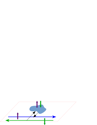
Figure 1: (color online). A pair of edge states tunnel-coupled to a conducting puddle in the bulk of the 2D topological insulator. The electron spin in the edge states is locked to the direction of motion, but the electrons in the puddle can flip it without restrictions.

Consider a pair of helical edge states with linear dispersion $\varepsilon_{p}=|p|\,v$ that connect the electron reservoirs, which are kept at externally controllable voltages. Each of the two directions of the electron momentum is locked to a definite spin projection, which is labeled by $\sigma=\pm 1$. The edge states are tunnel-coupled with electron or hole puddles that are formed in the bulk of the insulator because of large-scale potential fluctuations. We also assume that these puddles are sufficiently large to have a continuous spectrum and that the electrons in the puddles are also subject to a spin relaxation because of spin-orbit processes.

For simplicity, the interaction between the electrons in the edge states is neglected, as well as their interaction with the electrons in the puddle.

Hence the distribution functions $f_{\sigma}(x,\varepsilon,t)$ in the edge states obey the equation Lunde12

$$\left(\frac{\partial}{\partial t}+{\sigma}v\,\frac{\partial}{\partial x}\right)f_{\sigma}(x,\varepsilon,t)\\ =-\Gamma(x)\left[f_{\sigma}(x,\varepsilon,t)-F_{\sigma}(\varepsilon,t)\right]-e\,\frac{\partial u}{\partial t}\,\frac{\partial f_{\sigma}}{\partial\varepsilon},$$ (1)

where $\Gamma(x)$ is the rate of electron tunneling from point $x$ to the puddle, $F_{\sigma}(\varepsilon,t)$ is the spin-dependent distribution function of electrons in the puddle, and $u(x,t)$ is the electric potential. As the conductance of the puddle is much higher than that of the edge states, this distribution functions is spatially uniform inside it and obeys the equation

$$\frac{\partial F_{\sigma}}{\partial t}+\frac{1}{h\nu_{p}}\int dx\,\Gamma(x)\,[F_{\sigma}(\varepsilon,t)-f_{\sigma}(x,\varepsilon,t)]\\ +\frac{1}{2\tau_{s}}\,(F_{\sigma}-F_{-{\sigma}})=-e\,\frac{dU}{dt}\,\frac{\partial F_{\sigma}}{\partial\varepsilon},$$ (2)

where $\nu_{p}$ is the number of states in the puddle per unit energy, $\tau_{s}$ is the spin-relaxation time, and $U$ is the electrical potential of the puddle. In its turn, the time derivatives of $u$ and $U$ may be obtained through electric capacity of the edge state per unit length $c$, the puddle capacity $C$ and the charge-balance equations

$$\frac{\partial u}{\partial t}=-\frac{e}{c}\sum_{\sigma}\int\frac{d\varepsilon}{hv}\,\left[\sigma v\,\frac{\partial f_{\sigma}}{\partial x}+\Gamma\,(f_{\sigma}-F_{\sigma})\right],$$ (3)

$$\frac{dU}{dt}=\frac{1}{C}\,\frac{dQ}{dt}=\frac{e}{C}\sum_{\sigma}\int d\varepsilon\int_{0}^{L}dx\,\frac{\Gamma(x)}{hv}\,(f_{\sigma}-F_{\sigma}).$$ (4)

As $\nu_{p}$ and $\Gamma$ may be considered as energy-independent near the Fermi level, it is convenient to introduce the integrated quantities

$$n_{\sigma}(x,t)=\int\frac{d\varepsilon}{hv}\,[f_{\sigma}(x,\varepsilon,t)-f_{0}(\varepsilon)],$$ (5)

$$N_{\sigma}(t)=\int d\varepsilon\,\nu_{p}\,[F_{\sigma}(\varepsilon,t)-f_{0}(\varepsilon)],$$ (6)

where $f_{0}(\varepsilon)$ is the equilibrium Fermi distribution. Note that these are not the total electron concentrations because they take into account only the changes of electron number near the Fermi level and do not include the shifts of the bottom of the conduction band that result from the oscillating electric potential. One may exclude the quantity $u$ from Eq. 1 to obtain the equation for $n_{\sigma}$ in the form

$$\frac{hv\,\partial n_{\sigma}/\partial t-(e^{2}/c)\,\partial n_{-\sigma}/\partial t}{hv+e^{2}/c}\\ +\sigma v\,\frac{\partial n_{\sigma}}{\partial x}+\Gamma\,n_{\sigma}=\frac{\Gamma}{hv\nu_{p}}\,N_{\sigma}.$$ (7)

Furthermore, it is convenient to separate $N_{\sigma}$ into the charge and spin parts $N_{Q}=N_{+}+N_{-}$ and $N_{S}=N_{+}-N_{-}$. By adding and subtracting Eqs. 6 for $\delta N_{+}$ and $\delta N_{-}$ and making use of Eq. 4, one obtains the equations for these quantities in the form

$$\left[\frac{\partial}{\partial t}+\left(1+2\,\frac{e^{2}\nu_{p}}{C}\right)\frac{\varphi_{L}}{h\nu_{p}}\right]N_{Q}\\ =\left(1+2\,\frac{e^{2}\nu_{p}}{C}\right)\int_{0}^{L}dx\,\Gamma(x)\,(n_{+}+n_{-})$$ (8)

and

$$\left(\frac{\partial}{\partial t}+\frac{1}{\tau_{s}}+\frac{\varphi_{L}}{h\nu_{p}}\right)N_{S}=\int_{0}^{L}dx\,\Gamma(x)\,(n_{+}-n_{-}),$$ (9)

where the notation

$$\varphi_{L}=\int_{0}^{L}dx\,\Gamma(x)/v$$ (10)

denotes the dimensionless tunnel-coupling strength. This system of equations must be solved together with the boundary conditions

$$n_{+}(0)=\frac{eu(0)}{hv},\quad n_{-}(L)=\frac{eu(L)}{hv},$$ (11)

and the current at point $x$ can be calculated as

$$I(x,t)=ev\,[n_{+}(x,t)-n_{-}(x,t)].$$ (12)

III AC response

Calculate now the linear response of the system. We assume that the voltage drop with frequency $\omega$ is symmetrically applied to the terminals, i. e. $u(0)=\frac{1}{2}\,V\exp(-i\omega t)$ and $u(L)=-\frac{1}{2}\,V\exp(-i\omega t)$. Estimates show that for the edge states in HgTe quantum wells, $hv$ and $e^{2}/c$ are of the same order of magnitude. Therefore the terms with time derivatives in Eqs. 7 are much smaller than the ones with spatial derivatives and may be omitted if we restrict ourselves to $\omega\ll v/L$. Using the boundary conditions Eq. 11, one may write the solutions of these equations in the form

$$n_{+}(x)=\frac{eV}{2hv}\,K(x,0)$$

$$+\frac{N_{Q}+N_{S}}{2hv\nu_{p}} \int_{0}^{x}\frac{dx^{\prime}}{v}\,\Gamma(x^{\prime})\,K(x,x^{\prime}),$$ (13)

$$n_{-}(x)=-\frac{eV}{2hv}\,K(L,x)$$

$$+\frac{N_{Q}-N_{S}}{2hv\nu_{p}} \int_{x}^{L}\frac{dx^{\prime}}{v}\,\Gamma(x^{\prime})\,K(x^{\prime},x),$$ (14)

where

$$K(x,x^{\prime})=\exp\!\left\{-\int_{x^{\prime}}^{x}\frac{dx^{\prime\prime}}{v}\,\Gamma(x^{\prime\prime})\right\}.$$ (15)

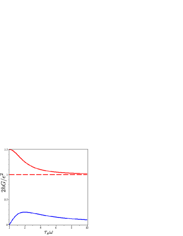
Figure 2: (color online). The real part (red curve) and imaginary part (blue curve) of the conductance vs. frequency for $\varphi_{L}=20$ and $h\nu_{p}/\tau_{s}=1$.

A substitution of these solutions into Eqs. 8 and 9 gives a system of equations

$$\Bigl{[}-i\omega+\left(\frac{1}{h\nu_{p}}+\frac{e^{2}}{C}\right)(1-e^{-\varphi_{L}})\Bigr{]}N_{Q}=0,$$ (16)

$$\Bigl{[}-i\omega+\frac{1}{\tau_{s}}+\frac{1-e^{-\varphi_{L}}}{h\nu_{p}}\Bigr{]}N_{S}=\frac{eV}{h}\,(1-e^{-\varphi_{L}}).$$ (17)

which suggests that $N_{Q}=0$. By substituting the value of $N_{S}$ from Eq. 17 into Eqs. 14 and 12, one obtains the expression for the current at the left and right terminals. Using the dimensionless spin-flip time

$$\eta=\tau_{s}\,\frac{1-e^{-\varphi_{L}}}{h\nu_{p}},$$ (18)

it may be presented in the form

$$I_{\omega}=\frac{e^{2}V}{2h}\left[1+e^{-\varphi_{L}}+\frac{(1-e^{-\varphi_{L}})\,\eta}{1+\eta-i\omega\tau_{s}}\right].$$ (19)

The real and imaginary parts of the frequency-dependent conductance are shown in Fig. 2. In the low-frequency limit $\omega\ll\tau_{s}^{-1}$, Eq. 19 gives

$$I_{dc}=\frac{e^{2}V}{2h}\,\frac{1+2\eta+e^{-\varphi_{L}}}{1+\eta},$$ (20)

which suggests that the dc conductance varies from $e^{2}/h$ to $e^{2}/2h$ and increase either with decreasing tunnel coupling $\varphi_{L}$ or increasing spin-flip rate $\tau_{s}^{-1}$. The contour plot of this quantity is shown in Fig. 3 as a function of $\varphi_{L}$ and the dimensionless spin-flip rate $h\nu_{p}/\tau_{s}$. In the high-frequency limit, it follows from Eq. 19 that

$$I_{hf}=\frac{e^{2}V}{2h}\,(1+e^{-\varphi_{L}}).$$ (21)

The high-frequency conductance also varies from $e^{2}/h$ to $e^{2}/2h$, but is independent of the spin-flip rate and is always smaller than the dc conductance. The high-frequency current is in phase with the ac voltage, and the phase shift between them appears only at $\omega\sim\tau_{s}^{-1}$.

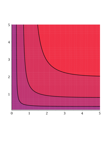
Figure 3: (color online). Contour plot of the dc conductance Eq. 20 as a function of $\varphi_{L}$ and $h\nu_{p}/\tau_{s}$. Brighter colors correspond to smaller values of conductance

IV Discussion

Though the response is calculated at frequencies much lower than the inverse time of flight of an electron between the terminals and the pileup of the charge is forbidden in the system, it still exhibits a dispersion related with spin imbalance in the puddle. At low frequencies, the conductance monotonically decreases as the coupling to the puddle and the spin-flip rate in it increase. Eventually it becomes equal to one half of the conductance in the absence of the puddle. This means that the puddle breaks the system into two independent quantum resistors, each with a conductance $e^{2}/h$. When connected in series, these resistors exhibit the conductance two times lower, i. e. $e^{2}/2h$. Should there be $m$ puddles strongly coupled to the edge states, the dc conductance would be $m+1$ times smaller than $e^{2}/h$. In some sense, increasing the frequency is equivalent to increasing the spin-flip rate, and it leads to a similar decrease of conductance. The single-puddle model involves three unknown parameters, i. e. $\varphi_{L}$, $\nu_{p}$, and $\tau_{s}$. All of them can be determined by comparing the experimental dispersion curve with Eq. 19. If it is not possible to measure the ac response in the whole frequency range, it may be possible to measure it in the dc regime and at a frequency well above $\tau_{s}^{-1}$, so one still can extract $\varphi_{L}$ and the product $h\nu_{p}/\tau_{s}$ by means of Eqs. 20 and 21.

The estimates Raichev12 show that the Fermi velocity in the edge states of HgTe quantum wells is about $5\times 10^{5}$ m/s. If the length of the edge state is one micron, the condition $\omega<v/L$ will be fulfilled up to the terahertz frequencies. It is more difficult to give reliable estimates of the spin-flip rate in the puddle. In low-temperature experiments on Au and Cu, the spin-flip time was $\approx 0.1$ ns Pierre03 . To the best of our knowledge, so far the ac response in 2D topological insulators was measured at a constant frequency of 2.5 THz and for several-micron long samples Kvon16 , which is marginal for testing the obtained results. One could extend the frequency limits for observing the predicted effects by choosing a shorter distance between the measuring probes and making an artificial puddle between them by approaching a charged STM tip or by selective doping. This would provide a test for the proposed model of the conductance suppression in the edge states of 2D topological insulators.

V Conclusion

We have calculated a current response to an ac voltage of a pair of edge states in a 2D topological insulators coupled by tunneling to a conducting puddle in its bulk, where the electrons can flip their spin. Our goal was to provide a means of experimental detection of such puddles. In a presence of such a puddle, the response exhibits a dispersion at the inverse spin-flip time in the puddle. Its real part decreases from the zero-frequency value to a smaller value, while its imaginary part exhibits a maximum at this frequency. By comparing the low-frequency and high-frequency response, one can determine the parameters of the puddle.

- (1) M. Z. Hasan and C. L. Kane, Rev. Mod. Phys. 82, 3045 (2010).
- (2) M. König, S. Wiedmann, C. Brüne, A. Roth, H. Buhmann, L.W. Molenkamp, X.-L. Qi, and S.-C. Zhang, Science 318, 766 (2007).
- (3) A. Roth, C. Brüne, H. Buhmann, L.W. Molenkamp, J. Maciejko, X.-L. Qi, and S.-C. Zhang, Science 325, 294 (2009).
- (4) G. M. Gusev, Z. D. Kvon, O. A. Shegai, N. N. Mikhailov, S. A. Dvoretsky, and J. C. Portal, Phys. Rev. B 84, 121302(R) (2011).
- (5) G. Grabecki, J. Wróbel, M. Czapkiewicz, L. Cywiński, S. Gieraltowska, E. Guziewicz, M. Zholudev, V. Gavrilenko, N. N. Mikhailov, S. A. Dvoretski, F. Teppe, W. Knap, and T. Dietl, Phys. Rev. B 88, 165309 (2013).
- (6) L. Du, I. Knez, G. Sullivan, and R-R. Du, Phys. Rev. Lett. 114, 096802 (2015).
- (7) I. Knez, C. T. Rettner, S-H. Yang, and S. S. P. Parkin, L. Du, R. R. Du, and G. Sullivan, Phys. Rev. Lett. 112, 026602 (2014).
- (8) J. Maciejko, C. Liu, Y. Oreg, X.-L. Qi, C. Wu, and S.-C. Zhang, Phys. Rev. Lett. 102, 256803 (2009).
- (9) Y. Tanaka, A. Furusaki, and K. A. Matveev, Phys. Rev. Lett. 106, 236402 (2011).
- (10) B. L. Altshuler, I. L. Aleiner, and V. I. Yudson, Phys. Rev. Lett. 111, 086401 (2013).
- (11) E. S. Tikhonov, D. V. Shovkun, V. S. Khrapai, Z. D. Kvon, N. N. Mikhailov, S. A. Dvoretsky, JETP Letters 101, 708 (2015).
- (12) J. I. Vayrynen, M. Goldstein, and L. I. Glazman, Phys. Rev. Lett. 110, 216402 (2013).
- (13) M. König, M. Baenninger, A. G. F. Garcia, N. Harjee, B. L. Pruitt, C. Ames, P. Leubner, C. Brüne, H. Buhmann, L. W. Molenkamp, and D. Goldhaber-Gordon, Phys. Rev. X 3, 021003 (2013).
- (14) S. Essert, V. Krueckl, and K. Richter, Phys. Rev. B 92, 205306 (2015).
- (15) P. P. Aseev and K. E. Nagaev, Phys. Rev. B 94, 045425 (2016).
- (16) R. J. Elliott, Phys. Rev. 96, 266 (1954).
- (17) A. W. Overhauser, Phys. Rev. 89, 689 (1953).
- (18) Z̆utić, J. Fabian, and S. Das Sarma, Rev. Mod. Phys. 76, 323 (2004).
- (19) A Boltzmann-like equation for the electrons in helical edge states coupled to impurity spins was also used by A. M. Lunde and G. Platero, Phys. Rev. B 86, 035112 (2012).
- (20) O. E. Raichev, Phys. Rev. B 85, 045310 (2012).
- (21) F. Pierre, A. B. Gougam, A. Anthore, H. Pothier, D. Esteve, and N. O. Birge, Phys. Rev. B 68, 085413 (2003).
- (22) Z. D. Kvon, K.-M. Dantscher, M.-T. Scherr, A. S. Yaroshevich, and N. N. Mikhailov, JETP Lettters 104, 729 (2016).