Do the contact angle and line tension of surface-attached droplets depend on the radius of curvature?
Abstract
Results from Monte Carlo simulations of wall-attached droplets in the three-dimensional Ising lattice gas model and in a symmetric binary Lennard-Jones fluid, confined by antisymmetric walls, are analyzed, with the aim to estimate the dependence of the contact angle on the droplet radius of curvature. Sphere-cap shape of the wall-attached droplets is assumed throughout. An approach, based purely on “thermodynamic” observables, e.g., chemical potential, excess density due to the droplet, etc., is used, to avoid ambiguities in the decision which particles belong (or do not belong, respectively) to the droplet. It is found that the results are compatible with a variation , being the contact angle in the thermodynamic limit (). The possibility to use such results to estimate the excess free energy related to the contact line of the droplet, namely the line tension, at the wall, is discussed. Various problems that hamper this approach and were not fully recognized in previous attempts to extract the line tension are identified. It is also found that the dependence of wall tensions on the difference of chemical potential of the droplet from that at the bulk coexistence provides effectively a change of the contact angle of similar magnitude. The simulation approach yields precise estimates for the excess density due to wall-attached droplets and the corresponding free energy excess, relative to a system without a droplet at the same chemical potential. It is shown that this information suffices to estimate nucleation barriers, not affected by ambiguities on droplet shape, contact angle and line tension.
e-mail address: das@jncasr.ac.in
I Introduction
Fluid nano-droplets on planar substrates are important in the context of heterogeneous nucleation 1 ; 2 ; 3 ; 4 ; 28 and of much recent interest nr1 ; nr2 ; nr3 , given that these have diverse applications in connection with microfluidics, nanofluidics, lithography, etc. 5 ; 6 . Their properties in (metastable) equilibrium are controlled by a subtle interplay of various surface tensions and the excess free energy attributed to the three phase contact line, the so-called line tension () 7 ; 8 ; 9 ; 10 ; 11 ; 12 ; 13 ; 14 ; 15 (see Fig. 1 for schematic depiction). However, theoretical and conceptual aspects of line tension are still controversially discussed (e.g. 10 ; 11 ; 12 ; 13 ) and attempts to estimate it experimentally have often led to results whose validity is still debated 9 .
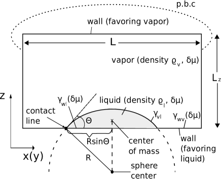
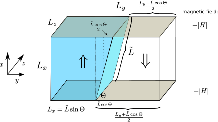
In this work we shall study various aspects related to wall-attached droplets via computer simulations, as previously done, see e.g. Refs. 16 ; 17 ; 18 ; 19 ; 20 ; 21 ; 22 ; 23 ; 49 . Unlike our previous works 18 ; 19 ; 20 ; 49 , we pay attention to the fact that for nano-droplets, in heterogeneous context, the contact angle () may depend on the droplet radius, e.g. because of the line tension 15 ; 24 ; 25 . This dependence needs to be taken into account self-consistently when one tries to estimate the line tension. Even if the line tension is disregarded, the contact angle of a nano-droplet may differ from its macroscopic value () for other reasons 11 . This problem can be avoided, at least in the framework of models possessing the particle-hole symmetry, like the Ising lattice gas system, between bulk coexisting phases, by considering a simulation geometry (shown in Fig. 2) 23 involving inclined planar interfaces between “antisymmetric” walls. We have demonstrated the viability of this approach for estimating contact angles also by lattice-based self-consistent field theory (SCFT), see e.g. 26 , for a symmetric binary mixture between two antisymmetric walls. However, as stated above, the objective of the present work is to explore the curvature dependence.
The sketch drawn in Fig. 1(a) implicitly uses a description appropriate for macroscopic droplets, such as water droplets on a car window visible by the naked eye: the droplet surface is drawn infinitely thin, and the contact line where it hits the wall is well-defined. However, it is doubtful that such a description can still be applied at the nanoscale without ambiguities resulting from the fact that on molecular scales interfaces are diffuse, there is no well-defined contact line then, and the nano-droplet shape may differ from the sphere-cap shape appropriate in the macroscopic limit (in the absence of gravity). In this work, we shall present a simulation approach that provides the possibility to extract properties such as contact angles, line tensions, etc., for liquid nanodroplets. At the same time, we shall demonstrate that it is possible to obtain estimates for the free energy barrier for the (heterogeneous) nucleation of such droplets and these estimates do not suffer from the ambiguities resulting from situation when the macroscopic description invoked in Fig. 1 (a) is taken too literally.
In Sec. II we shall concisely summarize the theoretical background of our work. In Sec. III we briefly describe our approach for the Ising lattice gas model, before showing that the resulting estimates for the contact angles indeed differ significantly from previous work 18 ; 19 , exhibiting a reasonably pronounced dependence on the droplet radius . This dependence is qualitatively consistent with standard predictions 15 ; 24 of a correction of order , when line tension estimates for planar interfaces 23 (see Fig. 2) are inserted. Due to anisotropy effects from the lattice, quantitative conclusions from our work are delicate, however. In addition, the lack in accuracy of the data 18 ; 19 does not allow us to obtain significantly improved estimates for the line tension. Sec. IV presents corresponding results for a symmetric binary () Lennard-Jones mixture, along with a description of the model and methods. Again quite noticeable differences with respect to the approximate approach of the previous work 20 are found. In this case also the results can be interpreted as an effective radius dependence of the contact angle, as mentioned above. Sec. V then discusses estimates for the -dependence of contact angle, obtained via a mean-field type approach 26 , coming via the wall tensions, for a lattice model of a binary mixture. Finally we summarize our findings in Sec. VI.
II THEORETICAL BACKGROUND
We now discuss the situation sketched in Fig. 1(a) in more detail. Note that in the thermodynamic limit, when the droplet radius of curvature , stable phase-coexistence between a liquid droplet (at density and surrounding vapor (at density is possible in the bulk. Then, of course, the chemical potential difference () between the (liquid) droplet and vapor (at bulk coexistence) is identically zero. As opposed to the spherical shape in the bulk, the droplet has sphere-cap shape at the surface (or wall) and the related contact angle is given by Young’s equation 8 ; 27
| (1) |
Here is the tension related to a planar liquid-vapor interface, while and are the surface tensions of vapor and liquid against the wall 23 .
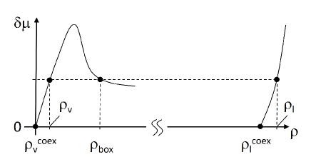
In the situation of interest, however, where is finite, we need to distinguish from . If we consider the droplet of Fig. 1 (a) to be nanoscopic, the chemical potential difference is positive [see the qualitative demonstration in Fig. 1 (b)]. The wall tensions and , in that case, will, in general, differ from their counterparts for – see Ref. 11 . In the framework of Monte Carlo (MC) simulations, it is easily possible to compute these wall tensions with the variation of (or of densities and , respectively) 29 ; 30 . At least for the model studied in Ref. 29 ; 30 the dependence of and on density is rather pronounced. Since decreases with density, while increases, this effect does not cancel out in the difference , which matters in Young’s equation. In addition, the excess free energy due to the line tension 7 ; 8 ; 9 ; 10 ; 11 ; 12 ; 13 ; 14 ; 15 plays crucial role. Some authors 24 ; 31 , hence, argued that Eq. (1) should be replaced by
| (2) |
Eq. (2) seems to be almost obvious as a consequence of the mechanical force balance at the contact line 15 . However, the real situation is not as simple, given that all interfaces are diffuse objects. In that situation, the notion of a contact line (particularly its length) may be influenced by the use of somewhat arbitrarily chosen “dividing surfaces” for the interfaces 10 . Even for a spherical droplet in the bulk, the “equimolar dividing surface” needs to be distinguished from the “surface of tension” 8 . Naturally, the length of the contact line, for a sphere cap, will depend on the choice of a dividing surface 10 ; 11 . In any case, when the dependence of the wall tensions on can be neglected, Eq. (2) can be reduced to the simpler result 15
| (3) |
Now we remind the reader of the basic concepts of the theory of heterogeneous nucleation 1 ; 2 ; 3 ; 4 . There one does not consider a small finite size system with linear dimensions comparable to the droplet radius as drawn in Fig. 1. Systems of interest, in fact, are macroscopic ones, being in a metastable vapor phase so that the liquid would be the stable phase), exposed to a wall in the grand-canonical ensemble. Then, , rather than the density in the system, is chosen as an independent variable. We emphasize at the outset that this will not be done in the simulations of the later sections. We will use the density, rather than the chemical potential, as the given independent variable.
Then one asks the question, assuming that a wall-attached sphere-cap shaped droplet with radius of curvature and contact angle forms, what would be its Gibbs free energy cost . Note that this question refers to a somewhat hypothetical situation, since such droplets are intrinsically unstable, out of equilibrium, and hence the use of equilibrium-type descriptions is somewhat questionable. However, in the end one is mostly interested in the position of the free energy maximum and its value only.
Hence, the Gibbs excess free energy of the droplet in Fig. 1 (a), relative to a state of the system at density [see Fig. 1 (b)], without a droplet, becomes (for small )
| (4) |
where is the length of the contact line. Furthermore, simple geometric considerations yield the volume , upper surface area and basal area of the droplet as
| (5) |
| (6) |
and
| (7) |
where is the Volmer-Turnbull (VT) function 1 ; 41 . The first term on the right hand side of Eq. (4) can be motivated by considering that the volume contribution to is typically written as , where is the pressure difference between the coexisting phases. The linear expansion of , by recognizing that density is a derivative of pressure with respect to the chemical potential, provides this form. A further assumption here is that the liquid and vapor densities, for the overall box density , are very close to the corresponding coexistence densities in the thermodynamic limit.
In this paper, we shall ignore the possibility that the vapor-liquid interfacial tension contains a curvature correction 8 ; 32 ; 33 ; 34 ; 35 ; 36 ; 37 ; 38 ; 39 ; 40 of order , which would make the contribution of the term related to the upper surface area in Eq. (4) of the same order as the line tension term 10 (when dependence in is ignored). In fact, for the models that we shall explicitly study, viz., the Ising lattice gas and a symmetrical binary Lennard-Jones fluid, no such curvature correction is expected – the leading correction there is proportional 36 ; 37 ; 44 ; 44pr to . Here we shall assume throughout that the radii of interest are large enough such that this curvature dependence of 8 ; 32 ; 33 ; 34 ; 35 ; 36 ; 37 ; 38 ; 39 ; 40 can be neglected. This fact we will justify later. For the lattice gas, however, it is a severe approximation to ignore the change in interfacial free energies due to lattice anisotropy (see e.g. Ref. 23 for a discussion). To avoid this problem, one should, in fact, choose for the latter model the vicinity of the critical point. Critical-like fluctuations then will get rid of the anisotropy, allowing one to have spherical droplets in the bulk and sphere-cap shaped droplets on planar walls. As a passing remark, for and we do not discard here the possibility of the leading correction being proportional to . In fact, we will see that which brings a correction linear in to the wall tensions.
When we consider a large spherical droplet in the bulk, we have the simpler result [cf. Eq. (4)]
| (8) |
Extremizing this expression, viz., by equating to zero, one obtains the standard theoretical expressions for the critical radius and associated nucleation free energy barrier related to the homogeneous nucleation 1 ; 2 ; 3 ; 4 . These are
| (9) |
When the contribution of the line tension to the droplet free energy is negligible, the standard result for the barrier, , against heterogeneous nucleation would result 1 ; 41 . If we assume that the contact angle takes its macroscopic value , then
| (10) |
the same VT function [see Eq. (5)], as in the case of volume, describing the reduction of the barrier in comparison with the homogeneous case.
In our previous simulation studies, attempting to extract the line tension 18 ; 19 ; 20 , the -dependence of the wall excess free energies as well as the change of the contact angle due to line tension [see Eqs. (2) and (3)] or other reasons, were neglected. Thus, Eq. (10) was simply replaced by an expression
| (11) |
that is believed to be correct only in the limit . However, taking Eq. (3) into account, one rather finds 15 , minimizing the free energy at constant droplet volume, that
| (12) |
Note that part of the correction due to the line tension is accounted for by replacing by in . This is seen by expanding Eq. (3) in leading order in and considering the first term on the right hand side of Eq. (12):
| (13) |
and
| (14) |
Accepting Eq. (12), one can show that for large the error made by Eq. (11) scales like :
| (15) |
Clearly, it is desirable to avoid Eq. (11), which for small , as used in previous simulations, is unjustified.
One purpose of the present work hence is to reconsider the simulations presented in Refs. 18 ; 19 ; 20 and attempt an analysis where both and are extracted from the simulation data by avoiding the use of Eq. (11) completely. Ref. 15 contains a detailed derivation of Eq. (12), promising “a rigorous thermodynamic formulation”. However, this derivation also ignores, to some extent like that of Eq. (11), both a possible dependence of on and , and the possible -dependence of the wall tensions, by the step from Eq. (2) to Eq. (3). In view of these approximations, in our proposed approach we keep in mind that the estimates should be done in such a way that it does not matter to what extent the difference is due to the line tension or due to the possible -dependence of the wall tensions.
A second purpose of the present work is to demonstrate that from a simulation of wall-attached droplets in equilibrium in finite systems in the canonical ensemble, as indicated in Fig. 1, one can obtain directly, as a function of , without the need to use the above equations. The idea is to study the density excess (see Fig. 1b) and the associated free energy difference between the two systems (with and without droplet) at the same .
III Ising model simulations and their analysis
We study the nearest-neighbor Ising model, on a simple cubic lattice, at a temperature , being the exchange constant and the Boltzmann constant. At this temperature, effects due to critical fluctuations are still negligible, given that the critical temperature is 42 . At the same time, the temperature is high enough so that the anisotropy effects on the interface are sufficiently small and thus, the droplet shape is almost spherical 43 .
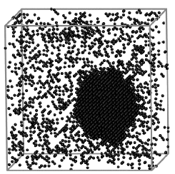
As depicted in Fig. 1 (a), we choose a geometry restricted in the -direction with linear dimension . At the bottom layer (), perpendicular to the latter direction, a short-range (-function) positive surface field acts. An antisymmetric boundary condition is created by putting a surface field of equal magnitude, but of opposite sign, at . On the other hand, periodic boundary conditions are applied in and directions, for which the linear dimensions and equal . We emphasize that the present approach, as described below, does not rely on a “microscopic” identification of which spins do belong to a droplet or not. While such an identification would be possible 43 , the strong fluctuations in the interfacial region [see Fig. 3 (a) for a picture in a bulk system] make such microscopic approach inconvenient. Before getting into the situation with a wall-attached droplet we provide a brief discussion with respect to the bulk.
In this work we employ a lattice variant of the Widom particle insertion method R1 , which is used to determine the chemical potential as a function of density [Fig. 3(c)]. This way nuclei of various shapes and sizes in a system can be probed. Integration of this curve with respect to density yields the free energy. Alternatively, one could employ a successive umbrella sampling technique R2 ; R3 by varying the overall composition in the system in a quasistatic manner 18 ; 19 . The method allows one to obtain the probability distribution for the density in the full range of the latter. From there one could obtain a free energy profile that contains information on the bulk coexistence values of densities as well as excess free energies for interfaces and lines. The chemical potential difference, , for a particular structure and size with respect to the bulk coexistence, could then be obtained from this free energy profile, by taking derivative with respect to density.
The basic principle one needs to apply then is that a liquid droplet of density coexists with a vapor of density at the same value of , as depicted in Fig. 1 (b). This, for a particular overall particle density, , inside the box, identifies and . The latter allows one to estimate the volume contribution of free energy, subtraction of which from the total value provides the excess free energy at . In addition, the corresponding radius , in a bulk system of volume , can be extracted from the lever rule as
| (16) |
for a spherical structure of the liquid droplet. This, of course, implicitly implies the use of an equimolar dividing surface between vapor and liquid so that there are no excess particles attributed to the interface. Since, for any choice of we know the appropriate value of and is straightforwardly calculated, the relation vs. can be constructed. The corresponding result in Fig. 3 (b), from bulk, implies an inverse relation between and for large enough . We make use of this relation in the situation with antisymmetric walls as well. In the confined case, with surface fields , we have
| (17) |
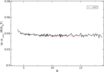
Of course, a crucial assumption of this approach is that also for radii that are finite, but much larger than the lattice spacing, the deviation of the shape of a droplet from a sphere-cap can be neglected. Only when this assumption is accurate, one can write the volume of the wall-attached droplet as 1 ; 41 . Assuming that Eq. (17) is accurate, for any given choice of we know [cf. Fig. 3 (c), for simulation results from confined systems], as well as the radius from bulk simulation [cf. Fig. 3 (b)]. Since at the obtained value of , and are also known, we can use this information to obtain from Eq. (17). This allows us to calculate hence the contact angle from Eq. (5). E.g., for the case and , this analysis yields , while . Although this difference is relatively small, it must not be neglected, contrary to the previous studies 18 ; 19 ; 20 . We emphasize that for this method of estimation of the contact angle of wall-attached sphere-cap shaped droplets for a chosen value of (or ) from Eq. (17), at a chosen value of , neither the knowledge of nor the knowledge of the line tension is required.
At this point we mention that the assumptions implied by Eq. (17) can be avoided if we only like to know the excess number of particles
| (18) |
due to the wall-attached droplet in the simulation box. This is of interest, since the “volume term” of nucleation theory can also be written as . We will make use of this later.
Fig. 4 now shows some central results obtained in the present paper, viz., estimates for as a function of , for various choices of , as indicated in the figure. Note that the values , shown for , are from the study of Block et al. 23 , for planar inclined interfaces in the Ising model. For two estimates of are included: the smaller values are obtained from Young’s equation, Eq. (1), while the upper ones are from a “first principle’s” approach 23 . The latter method takes the effects of lattice anisotropy on the interfacial free energy, , of the lattice gas model, into account. This lattice effect is expected to become negligible when the temperature approaches the critical value, but turns out to yield a difference of a few degrees for the contact angles at the considered temperature . In any case, it is remarkable to observe that in the accessible range of radii the contact angles of the droplets are always smaller than both the estimates for . Roughly, the variation of with is compatible with a linear behavior, as expected from Eq. (3), when [see Eq. (13)].
As a first qualitative test of Eq. (3), in Fig. 4 we plot the result of this equation, using for the estimate , and for the estimates due to Block et al. 23 for planar inclined interfaces that are hitting a flat wall. It is seen that the resulting curves that use from Eq. (1) always fall slightly below the actual data for , while the other predictions on , taking the anisotropic feature of the interfacial tension into account, overestimate it. Clearly, the effects due to this anisotropy, which also is expected to cause a slight but systematic deviation from sphere shape 43 , preclude a more precise test of Eq. (3).
Next we consider the numerical computation of the excess free energy of the droplet, making use of a thermodynamic integration procedure
| (19) |
using data such as shown in Fig. 3 (c). Eq. (19) is the excess free energy due to the droplet per lattice site, in the canonical ensemble. Note that Eqs. (4) and (8) refer to the grand-canonical ensemble. In the canonical ensemble the volume term proportional to is not present. So we pick up from just the surface and line tension contributions. Since there is a one-to-one correspondence between and and hence , the quantity can be re-interpreted in terms of the surface excess free energy . Recently, it has been recognized that the translational entropy of the droplet in the simulation box should not be ignored 40 , if one compares data obtained from simulations [Eq. (19)] with theoretical estimates. For a wall attached droplet, we hence should add to to obtain . For this amounts to about .
In previous work it was assumed that can be interpreted as 18 ; 19
| (20) |
which leads to the barrier for heterogeneous nucleation – see Eq. (11). For an understanding on the effects of curvature dependence of , by neglecting the correction due to the line tension, the surface part of the free energy of the wall-attached droplet simply could be written as
| (21) |
At , the data of Winter et al. 18 ; 19 are compatible with
| (22) |
with and =1.85 lattice units. Note that for this result implies for the total free energy of a droplet in the bulk to be [cf. Eq. (8)]
| (23) |
Hence the result for [see Eq. (9)], resulting from , is not truly affected by this correction due to the -dependence of .
Naively one might correct Eq. (20), by rewriting it after taking the actual contact angles into account, as
| (24) |
where is the radius of the circular contact line. The resulting estimates for are plotted in Fig. 5, versus . Unfortunately, the scatter of the resulting data is large and not systematic, indicating that the statistical accuracy with which is obtained from Eq. (19), as well as the accuracy of , does not suffice for a meaningful analysis of the dependence of the line tension on the circular radius and contact angle . It is seen that the results for a planar interface (from Block et al. 23 ) increase slightly from to , when is varied. The data for extracted from the droplets seem to be only very roughly consistent with this trend, but probably lack the necessary accuracy to allow for a clear conclusion. But it is evident that the dependence of on and is not very strong. However, if Eq. (12) would be used to analyse the data for , the absolute magnitude of would be twice as large, making it completely incompatible with the limiting behavior for (planar interface).
At first sight, all these facts are surprising. However, while the droplet surface is a two-dimensional object here, the contact line is one-dimensional, and hence much larger finite-size corrections due to fluctuations can be expected. When, for the sake of analogy, we consider the droplets in the two-dimensional Ising model, where the droplet “surface” also is a one-dimensional line, a much larger size effect than in [see Eq. (22)] occurs 34 ; 40
| (25) |
Returning now to the starting point of our discussion, introducing the line tension from the mechanical equilibrium of the contact line, Eq. (2), we note that the wall tensions, to first order in , can be written as
| (26) |
and
| (27) |
which yield [see Eqs. (1) and (2)]
| (28) |
where is the difference in the adsorption from the vapor and the liquid . Using Eq. (9), to replace by , we note that the first term on the right hand side of Eq. (28) is of the same order as the second term. Still another expression has been derived in Ref. 10 :
| (29) |
where a further correction involving the Tolman length 32 has been omitted. Eq. (2) [or Eq. (28)] is compatible with Eq. (29) only when depends neither on nor on , which clearly is not true.
While our work hence cannot fully clarify the problems relating to the line tension, we do get from our study valid and reasonably accurate results for the barrier against heterogeneous nucleation as
| (30) |
where , as noted above. Fig. 6 shows a log-log plot of versus . For and we include a comparison with the prediction of the classical theory [see Eqs. (9) and (10)],
| (31) |
One sees that the actual barriers, say for , are about a factor 1.6 lower, though the general trend is similar. If there is no line tension effect, one would also have the relation . For this estimate also has been included, with the above choice of , and one sees that this still amounts to an overestimation. Similar, but somewhat larger, discrepancies apply to the other choices of as well. In fact the simulation results for are expected to be smaller than the predictions. This is because the negative values of line tension (see Fig. 5) reduce the barriers.
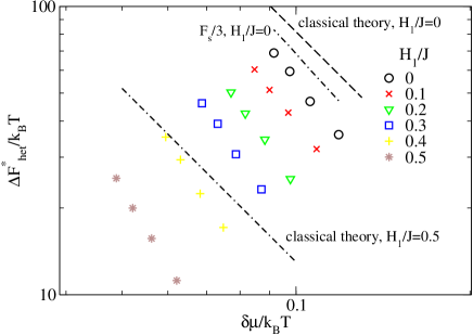
Unfortunately, for each choice of only a rather restricted range of is accessible: this happens because we cannot use data for [in Figs. 1(b) and 3(c)] that are close to the peaks in the vs. curve; as is well known, these peaks correspond to the droplet evaporation/condensation transition 18 ; 19 ; 36 . Likewise, data for too large (where in the curves of Fig. 3(c) an inflection point is seen) cannot be used either; there the droplet shape changes from sphere cap to cylinder cap shape (stabilized by the periodic boundary conditions). But the range of barriers that is accessible here (about is in a range that would be physically significant. Note that the regime of much larger droplets, for which the theory outlined in Sec. II is presumably more accurate, would relate to much larger barriers which are physically irrelevant.
IV Analysis of simulation results for the symmetric binary fluid
The inter-particle interaction in the binary () fluid mixture, in this section, is defined in terms of the Lennard-Jones (LJ) potential (, and being the positions of particles and , respectively)
| (32) |
with
| (33) |
For the interaction strength, is chosen differently 20 ; 44 ; 45 , viz., , to facilitate liquid-liquid phase separation, as opposed to the choice of equal diameter () for all combinations of particles. To improve the speed of the simulations, it is preferable to cut the potential at some distance , for which we choose . But for molecular dynamics simulations (that were performed 45 ; 48 for understanding of various equilibrium and nonequilibrium dynamical properties of this model) it became essential to make the potential and also the force continuous at . This can be achieved by modifying the LJ potential as 20 ; 44 ; 45
| (34) |
which we used for the present study.
Temperature in this model has the unit , all lengths will be measured in unit of and the dimensionless density is calculated as . Here is the total number of particles (, and being the numbers for and particles) and , where () is the box length along the Cartesian direction . In the following, for convenience, we set , and to unity. We may, however, explicitly use them when verification of an expression with respect to dimension is required. We set and perform all simulations at , which is far below the critical temperature () of the model 45 ; 48 . The bulk interfacial tension for this temperature was found to be 20 . This model shares with the Ising model the advantage of a strict symmetry between the two coexisting phases, thus, the critical composition is identically set at composition of and particles. The model has the further advantage that the interfacial tension is fully isotropic, due to the off-lattice character.
In order to realize a situation with antisymmetric walls, similar to Fig. 1(a), wall potentials and , acting on the two types of particles, are chosen as 20 ; 49 ; 44
| (35) |
| (36) |
where (), as in the previous section, again is the coordinate perpendicular to the walls. An offset , for the origin of the wall potentials, is used, such that the latter is finite everywhere inside the box. Both walls exert the same repulsive potential (with ) on both types of particles, so that no particles can leave the system by penetrating the walls. Note that periodic boundary conditions are used in the and directions, with . The attractive potential, with prefactor [see the last terms on the right hand sides of Eq. (35) and (36)], acts on particles only from the wall at , while for particles it comes only from the wall at . This is the analog of the antisymmetric surface field in the Ising model (Fig. 1). However, while for the lattice model the wall potential was chosen to be of strictly short range, here we do not use any cut-off for the wall potentials.
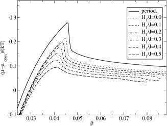
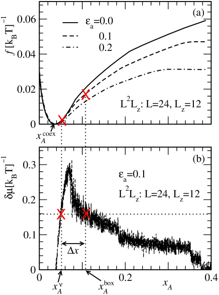
Our Monte Carlo (MC) simulations 42 with this model, of course, consider local displacement moves of the particles. For such trial moves we randomly choose particles and change their Cartesian coordinates, again randomly, such that the displacement lies in the range . When , and are kept fixed, this provides realization of the canonical ensemble 42 . For the purpose of efficiently obtaining the effective free-energy density , (), the variable analogous to for the vapor-liquid case in the previous section, being the concentration of particles, in the two-phase coexistence region, we use (successive) umbrella sampling method 20 ; R2 . Thus, in addition to using displacement as trial moves, we have used identity switches () as well. For such moves we have chosen a particle randomly, identified its type and changed it. This calls for an introduction of difference between chemical potential between and particles in the Boltzmann factor, for the execution of the Metropolis algorithm 42 . However, along coexistence such difference is identically zero. Umbrella sampling MC simulations, in addition to providing information on the coexistence curve, helps obtaining the accurate probability distribution for the fluctuation of over the whole spectrum () of the latter. From such probability distribution the free energy curve, as a function of , can be straightforwardly obtained, for bulk as well as for the confined systems. At the chosen conditions, the system in the bulk exhibits two-phase coexistence for lying between and . For the confined system, we find [see Fig. 7 (a)].
Fig. 7 shows examples for both [see part (a)] and [see part (b)]. The latter can be obtained from the derivative of with respect to . While in part (a) we include results from three choices of , including , part (b) contains results only for , since chemical potential difference, vs. , is shown only to demonstrate the method. For both the quantities we have included results only for a part of the overall range, that is relevant for the analysis. It is clear from Fig. 7 (a) that, as expected, with the increase of the energy barrier decreases, due to enhancement of favorable wetting condition. The regions between the first two knees of the free energy curves correspond to sphere-cap structure of droplets rich in particles, radius of which increases with the increase of . By moving towards right one will encounter transitions to cylinder-like and slab-like structures, below the wetting transition. These are not of interest in this work. In this figure we have outlined the estimation of the concentration difference , from which, via a relation analogous to Eq. (17), the actual contact angle is extracted. Specifically, is related to the (wall attached) droplet volume () as
| (37) |
Thus, one can straightforwardly calculate , thus, , as a function of , by obtaining information on the volume reduction compared to a droplet in the bulk with same radius. This, of course, requires the knowledge of . Estimation of the latter we discuss below, though already described in the previous section. In fact, missing information in Sec. III, if any, can be obtained from the details below.
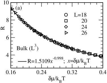
Due to the pronounced statistical fluctuations of the chemical potential difference, the estimation of the latter, as well as of , for chosen states , has to be done with care. To facilitate working with smooth curves, we have taken help of fitting of the simulation data to nonlinear functions. E.g., the ascending branch of vs. plot was fitted to polynomial forms of degree four, while the descending branch was fitted to power laws. For the corresponding radius needed here, we use the relation between and found in the bulk. Here we make use of the fact that droplets of same exist at same chemical potential difference, irrespective of whether they are attached to the wall or not. Related results are presented in Fig. 8 (a). To avoid the finite-size effects we have considered only overlapping data from different system sizes, as shown. For this purpose also we have used the fitting method – see caption for details. There, essentially an inverse relation between and emerges. This fact is consistent with our discussion above [see Eqs. (8) and (9), along with related text] with respect to vapor-liquid transition, concerning the homogeneous nucleation theory for critical radius and corresponding energy barrier. Even the prefactor () is almost theoretically perfect, given that for the binary mixture
| (38) |
where is interfacial tension.
Here we mention that in an earlier work 20 we had obtained by using , calculated from an independent study that used a thermodynamic integration method, in the expression . This and subsequent method did not naturally allow us to obtain any curvature dependence of and .
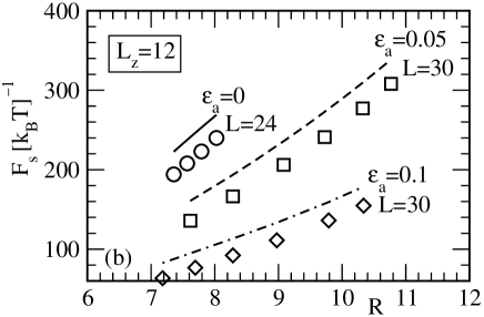
From Fig. 7 (a) we can extract the actual (surface) excess free energy due to the droplet, from the difference () between for the states at and , as a function of , and thus, of , given that . This can be compared with the result one would obtain if the line tension effects were negligible [see lines of various types in Fig. 8 (b)], i.e., with , using the actual contact angles found from the knowledge of . The simulation results for are presented as symbols in Fig. 8 (b). One sees that the actual surface excess free energies are clearly smaller, indicating the presence of a negative line tension.
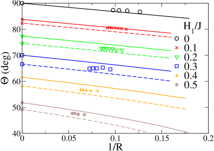
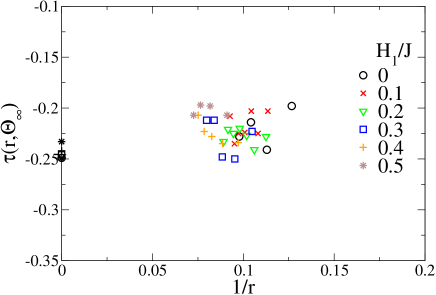
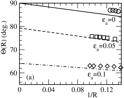
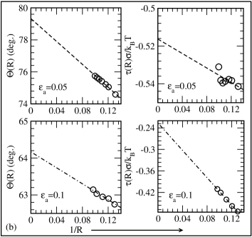
The line tension can be calculated from the discrepancies between the continuous lines and the symbols in Fig. 8 (b), by using Eq. (11). Our best estimates for both contact angle and line tension are shown in Fig. 9, vs. . In Fig. 9 (a) we show contact angles from three choices of . Note that for one expects . In this figure we have also included the results that one would obtain from Eq. (3). While Eq. (3) gives qualitatively the right trend, a good quantitative agreement is not obtained. Unfortunately, only a rather small range of values for is accessible for our analysis. Hence, as in the case of the Ising model, rather tentative conclusions on the dependence of the line tension on contact angle and radius can be inferred. However, we can conclude rather safely that the contact angle for small wall-attached droplet is always significantly smaller than its asymptotic value. Hence, as mentioned above, the results for the line tension obtained previously in Ref. 20 , for this model, suffer from systematic errors due to this change of contact angle for small droplets.
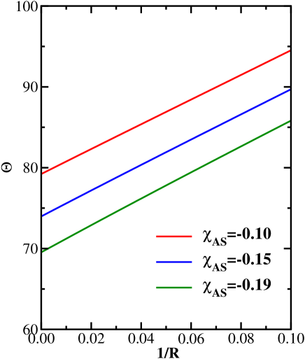
We add here that for this model we have an estimate of from planar interface available only 20 ; 49 for . For other values of we have obtained thermodynamic limit value of from extrapolations of -dependent data of to . (Note that these plots are slightly different from the Ising lattice gas case for which we have plotted as a function of , not .) This procedure is shown in Fig. 9 (b) – see the right frames. In the left frames of this figure we have shown magnified pictures for the radius dependence of contact angle for the nonzero values of . The values of obtained from here are used for the theoretical lines of Fig. 9 (a).
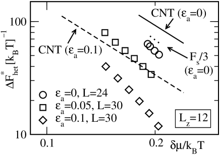
Before closing this section, in Fig. 10 we present results for the barriers for heterogeneous nucleation, i.e., we plot versus , for different values of . These results are analogous to Fig. 6 (that corresponds to the lattice gas model). Here also we compare the simulation results with the classical theory (marked as CNT). The discrepancies between theory and simulation again imply negative line tension. Here we have not included the entropic contribution to .
V Mean-field type calculation for the dependence of contact angle on the chemical potential difference
In this section, we return to the Ising model between antisymmetric walls, and reinterpret the two spin values as particles of type A and B. Being interested in temperatures far below the bulk critical temperature, it is tempting to study contact angles within a mean-field type approximation. This is to obtain clarification to what extent the variation of the line tension with droplet radius, implied by the results of the previous sections, is a fluctuation effect, or simply an effect due to the dependence of wall free energies on the chemical potential difference between the droplet and its environment.
A convenient construction of mean-field theory for inhomogeneous lattice problems is the Scheutjens-Fleer formulation 46 of self-consistent field theory (SCFT). While SCFT was originally intended for polymeric systems, it can be applied to a lattice model for binary mixtures as well. Since SCFT directly yields the free energy of the system, one can obtain wall excess free energies straightforwardly 26 ; 46 . Denoting the normalized interaction energy (Flory-Huggins parameter) as
| (39) |
where is the coordination number of the simple cubic lattice, we note that criticality in the bulk would occur for . So the regime of interest is . Similarly, one can define the normalized interaction energy of -particles with -particles forming the wall as
| (40) |
and likewise, the normalized interaction energy of -particles with -particles () can be defined by replacing with everywhere in the above equation.
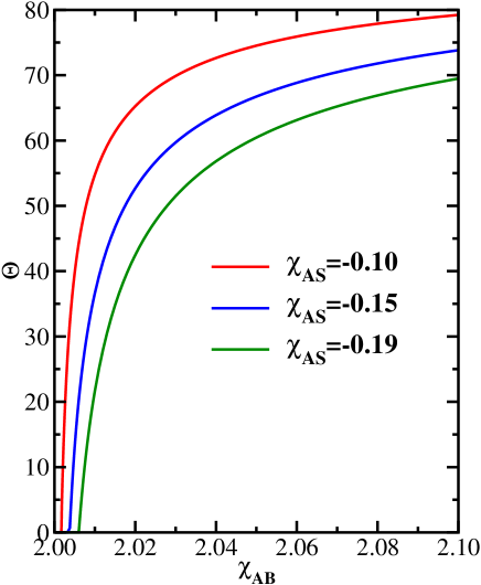
Using walls, which attract either -particles with attraction strength or -particles with attraction strength , one can both obtain wall excess free energies at coexistence conditions, and study also antisymmetric systems with an inclined interface, similar to Müller et al. 26 . Using Young’s equation, Eq. (1), one readily obtains the contact angle as a function of these energy parameters (see Fig. 11 (a) as an example). One sees that vanishes when the wetting transition occurs but for already rather large values of occur. Hence we shall focus on the -dependence of for this case in the following.
For the calculation of wall tensions and from this mean-field theory, one uses a geometry, with periodic boundary conditions invoked in and directions, and on a mean-field level only inhomogeneity in -direction occurs. Thus the implementation of SCFT for this calculation is rather straightforward.
In order to carry out a meaningful comparison with the result of the previous sections, we assume chemical potential differences related to a droplet radius according to Eq. (38). For the chosen example (Fig. 11) with we have and . Being only interested in the leading behavior for large , it suffices to expand the wall tensions at the coexistence curve according to Eqs. (26) and (27) by identifying the liquid phase with -rich phase and the vapor phase with the -rich phase. From Eqs. (38), (26) and (27) we immediately conclude
| (41) |
where , computed at coexistence. Note that Eq. (41) holds beyond mean field, for , if the dependence on wall excess free energies on is the only reason for a difference between and .
In Eq. (41), simply is the result according to Young’s equation, applying for . Clearly, mean-field theory predicts that the dependence of the contact angle on the chemical potential difference , and hence via Eq. (38) indirectly on , is a rather pronounced effect! This finding confirms the concerns raised by Schimmele and Dietrich 11 that one has to be very careful when one wishes to associate the radius dependence of the contact angle of wall attached sphere-cap shaped droplets with the “true” line tension.
It is tempting to use a higher-dimensional version of this mean-field theory for computing the line tension 47 . However, due to lattice effects (interfaces in mean-field theory stay non-rough up to bulk criticality) this is rather difficult to implement, and hence not done here.
VI Discussion
In this paper, we have presented a re-analysis of simulation data, that were used in two earlier attempts 18 ; 19 ; 20 , to extract estimates for the contact angle of wall-attached sphere-cap shaped droplets and the line tension related to the corresponding three-phase contact, by paying attention to a dependence on the droplet radius. In the previous works, a heuristic assumption was made that the contact angle of these droplets is the same as the contact angle of macroscopic droplets, which can be estimated independently from Young’s equation. As a matter of fact there is no theoretical basis for this assumption, and hence it is clearly desirable to avoid it. We show here that this task can indeed be achieved by the simulation strategy of the previous work 18 ; 19 ; 20 , by using the explicit knowledge of the relation between the droplet radius of curvature and the chemical potential difference that characterizes the equilibrium between the system containing the droplet and bulk phase coexistence, and the excess density due to the droplet.
However, a crucial approximation which remains is that for the excess volume of the wall-attached droplet a sphere-cap shape is accurate, i.e., corrections to Eq. (5) due to deviations of the droplet shape near the contact line are sufficiently small so that they can be neglected. This is plausible since only a volume of order , where is a length of the order of molecular distances, should be affected. Hence for the volume of the sphere cap this is a correction of order . So we expect a correction for our contact angle of order , while the corrections that are found and discussed here are of order , much stronger than above errors can bring in. In the case of the lattice gas model, a further caveat is that the anisotropy of the lattice also causes systematic deviations of droplet shapes from being spherical (or sphere-cap, respectively). But at the chosen temperature these anisotropy effects should be very small.
If these assumptions are accepted, direct estimation of as a function of is possible. We have interpreted the deviations between and in terms of line tension effects, notwithstanding the knowledge that in view of the criticisms raised by Schimmele et al. 10 ; 11 this is doubtful. For the Ising model, an estimation of the dependence of the “true” line tension (referring to macroscopic planar interfaces) on contact angle is available 23 , and this dependence is incompatible with previous estimates resulting from droplets 18 ; 19 . This led to a motivation for the present work. However, the present results are hardly compatible with the implicit assumption of 15 , viz., the line tension is a true constant, i.e., does not depend upon and . We have, however, provided evidence, already on the mean-field level, that the dependence of contact angles (even for ) on the chemical potential in the system (for finite , must be nonzero in equilibrium) is of a similar magnitude as the dependence attributed to line tension effects.
The above findings agree with concerns raised by Schimmele and Dietrich 10 ; 11 . Of course, computer simulations suffer from well-known problems such as finite size effects, statistical errors, incomplete equilibration, etc. 42 . Hence it is not straightforward to clarify all the issues that our work raises. However, other numerical approaches such as density functional theory 14 seem to provide a rather strong variation ( for small , and also raise questions.
In conclusion, although the concept of the line tension was introduced by Gibbs more than a century ago 7 , its numerical estimation by experiment, simulation and theory still is difficult. An interesting point is that for both the models, lattice gas and binary Lennard-Jones, the variation of the contact angle of droplets seems to be compatible with a linear behavior in .
Finally, we again like to emphasize that our simulation approach yields directly estimates for the barrier that needs to be overcome in the heterogeneous nucleation events, which are not at all affected by uncertainties in our knowledge of contact angles and line tensions. These estimates (e.g. Fig. 6 and Fig. 10) do not make any assumption what the actual droplet shapes are, but rely fully on our estimates of the excess density due to the droplet and associated free energy excess.
Acknowledgment
SKD acknowledges the Marie Curie Actions Plan of European Commission (FP7-PEOPLE-2013-IRSES grant No. 612707, DIONICOS), International Centre for Theoretical Physics, Trieste, and Johannes-Gutenberg University of Mainz for partial supports.
References
- (1) Volmer M 1939 Kinetic der Phasenbildung (Dresden: Th. Steinkopff)
- (2) Zettlemoyer AC (ed.) 1969 Nucleation (New York: Dekker)
- (3) Kashchiev D 2000 Nucleation: Basic Theory with Applications (Oxford Butterworth-Heinemann)
- (4) Kelton KF and Greer AI, 2009 Nucleation (Oxford: Pergamon)
- (5) Dietrich S 1988 Phase Transitions and Critical Phenomena Vol XII, ed C. Domb and J.L. Lebowitz (New York: Academic) p1
- (6) Jamali V, Biggers EG, van der Schoot P and Pasquali M 2017 Langmuir 33 9115
- (7) Seveno D, Blake TD and Coninck JD 2013 Phys. Rev. Lett. 111 096101
- (8) Jiang H, Müller-Plathe F and Panagiotopoulos AZ 2017 J. Chem. Phys. 147 084708
- (9) Tableing P 2010 Introduction to Microfluidics (Oxford: Oxford University)
- (10) Natelson D 2015 Nanostrucutres and Nanotechnology (Singapore: World Scientific)
- (11) Gibbs JW 1961 The Scientific Papers, Vol 1 (New York: Dover)
- (12) Rowlinson R and Widom B 1982 Molecular Theory of Capillarity (Oxford: Oxford University)
- (13) Amirfazli A and Neumann AW 2004 Adv. Colloid Interface Sci. 110 121
- (14) Schimmele L, Napiorkonski M and Dietrich S 2007 J. Chem. Phys. 127 164715
- (15) Schimmele L and Dietrich S 2009 Eur. Phys. JE 30 427
- (16) Velarde MG 2011 Eur. Phys. J Special Topics 197 3
- (17) Sefiane K 2011 Eur. Phys. J Special Topics 197 151
- (18) Zhou D, Zhang F, Mi J and Zhang C 2013 AI Che Journal 59 4390
- (19) Singha SK, Das PK and Maiti M 2015 J. Chem. Phys. 142 104706
- (20) Ingebrigsten T and Toxvaerd S 2007 J. Phys. Chem. C 111 8518
- (21) Shi B and Dhir VK 2009 J. Chem. Phys. 130 034705
- (22) Winter D, Virnau P and Kinder K 2009 J. Phys.: Condens. Matter 21 464118
- (23) Winter D, Virnau P and Binder K 2009 Phys. Rev. Lett. 103 225703
- (24) Das SK and Binder K 2010 Europhys. Lett. 92 26006
- (25) Das, SK and Binder K 2011 Molec. Phys. 109 1043
- (26) Wegs JH, Marchand A, Andreotti B, Lohse D and Snoeijer H 2011 Phys. Fluids 23 022001
- (27) Becker S, Urbanek H M, Horsch M and Hasse H 2014 Langmuir 30 13606
- (28) Block BJ, Kim S, Virnau P and Binder K 2014 Phys. Rev. E90 062106
- (29) Navascués G and Tarazona P 1981 J. Chem. Phys. 75 2441
- (30) Gaydos J and Neumann A 1987 J. Colloid Interface Sci. 120 76
- (31) Müller M, Albano EV, and Binder K 2000 Phys. Rev. E62 5281
- (32) Young T 1805 Phil. Trans Roy Soc. London 95 65
- (33) Statt A, Winkler A, Virnau P and Binder K 2012 J. Phys.: Condens. Matter 24 46122
- (34) Statt A 2012 Wetting Behavior of the Liquid-Vapor Phase Coexistence of a Colloid-Polymer Mixture (Mainz: Johannes Gutenberg Universität, Diplomarbeit unpublished)
- (35) Borovka L and Neumann AW 1977 J. Chem. Phys. 66 5464
- (36) Turnbull D and Vonnegut B 1952 Ind. Eng. Chem. 44 1292
- (37) Tolman RC 1949 J. Chem. Phys 17 333
- (38) Günther NJ, Nicole DA, and Wallace DJ 1980 J. Phys. A: Math. Gen 13 1755
- (39) Ryu S and Cai W 2010 Phys. Rev. E81 030601 (R)
- (40) Ryu S and Cai W 2010 Phys. Rev. E82 011603
- (41) Block BJ, Das SK, Oettel M, Virnau P and Binder K 2010 J. Chem. Phys. 133 154702
- (42) Das SK and Binder K 2011 Phys. Rev. Lett. 107 235702
- (43) Tröster A, Oettel M, Block B, Virnau P, and Binder K 2012 J. Chem. Phys. 136 064708
- (44) Prestipino S., Laio A and Tosatti E 2013 J. Chem. Phys. 138 064508
- (45) Tröster A, Schmitz F, Virnau P and Binder K 2017 J. Phys. Chem. B (in press)
- (46) Das SK 2015 Molec. Simul. 41 382
- (47) Fisher MPA and Wortis M 1984 Phys. Rev. B 29 6252
- (48) Landau DP and Binder K 2015 A Guide to Monte Carlo Simulation in Statistical Physics, 4th ed. (Cambridge University)
- (49) Schmitz F, Virnau P and Binder K 2013 Phys. Rev. E87 053302
- (50) Widom B 1983 J. Chem. Phys. 39 2808
- (51) Virnau P, Müller M 2004 J. Chem. Phys. 120 10925
- (52) Virnau P, Müller M, MacDowell LG, Binder K J. 2004 Chem. Phys. 121 2169
- (53) Das SK, Fisher ME, Sengers JV, Horbach J and Binder K 2006 Phys. Rev. Lett. 97 025702
- (54) Roy S and Das SK 2011 Europhys. Lett. 94 36001
- (55) Fleer GJ, Cohen Stuart MA, Scheutjens JMH, Casgrove T, and Vincent B 1993 Polymers at Interfaces (London Chapmann and Hall)
- (56) Ibagon I, Bier M, and Dietrich S 2016 J. Phys.: Condens. Matter 28 264015