On the Use of the Observability Gramian
for Partially Observed Robotic Path Planning Problems^∗

Abstract

Optimizing measures of the observability Gramian as a surrogate for the estimation performance may provide irrelevant or misleading trajectories for planning under observation uncertainty.

I Introduction

The Observability Gramian (OG) is used to determine the observability of a deterministic linear time-varying system [1, 2, 3]. For such systems, the properties of the OG have been well-studied [1, 4, 5]. When sensors provide noisy stochastic measurements, the state is only partially observed. The general problem of planning under process and observation uncertainties has been formulated as such a stochastic control problem with noisy observations. The solution of this problem provides an optimal policy via the Hamilton-Jacobi-Bellman equation [6, 7]. However, the computational hurdle for finding a solution to these equations has necessitated the study of a variety of methods to approximate the solution [8, 9, 10, 11]. One approach has been to maximize the estimation performance by planning for trajectories that can exploit the properties of observation, process and a priori models. We examine the appropriateness or lack thereof of methods based on the OG, and show that they can provide misleading trajectories.

Borrowed from deterministic control theory, the OG has been exploited in order to provide more observable trajectories, particularly in trajectory planing problems [12, 13, 14, 15, 16, 17, 18]. In the special case of a diagonal observation covariance with the same uncertainty level in each direction [1], the Standard Fisher Information Matrix (SFIM) does reduce to the OG. Indeed the usage of the OG in filtering problems has been justified through its connections to the SFIM and its relations to the parameter estimation problem [19, 13]. In fact, tailored to the parameter estimation problem, the SFIM only addresses the amount of information in the measurements alone [1], and neglects both the prior information and process uncertainty. Closely-related approaches are the methods that base their planning on the observation model or the likelihood function [8, 20], and the analysis of this paper can be helpful in providing a better understanding of those problems.

In contrast, the Posterior FIM (PFIM), whose inverse coincides with the Posterior Cramér-Rao Lower Bound for the estimation uncertainty in a general stochastic problem [21], can capture the history of evolution of uncertainty in the problem. In particular, for a linear system, it has been shown that the Riccati equations for the covariance evolution of the state estimation resulting from the Kalman Filter (KF) coincide with evolution of the PFIM in the form of the inverse covariance or the information filter [21, 22, 23, 24]. Indeed, it is only this measure that can capture the entire information required to calculate the optimal policy along with the nominal trajectory of a stochastic system. It is therefore no surprise that these equations provide the evolution of the information state (the posterior or conditional distribution of the state given the entire history of actions and observations) as the sufficient statistic for decision-making through the Bayesian filtering equations.

In this paper, through a series of analytic and numerical examples, we show that the observability Gramian does not generally provide an appropriate solution for the problem of planning under uncertain observations. We provide examples for two commonly used nonlinear observation models including the range and squared-range observation models that provide noisy information regarding the state of the system with respect to a set of information sources or landmarks. The examples show that the OG is insensitive to the uncertainty parameters of the problem, with none of the three main covariances, i.e., process, observation or initial, appearing quantitatively. Similarly, we show that the SFIM also suffers the same problems as the OG.

The numerical examples illustrate the performance of simple planning problems when a measure of the OG (or SFIM in special case) is utilized as the optimization objective. In these examples, the trace of the error covariance, which represents the sum of mean squared errors along the trajectory, is used as the measure of performance of trajectory. In each example, the OG-based trajectory’s performance is evaluated against both an initial trivial path and the optimized path with respect to the trace of the covariance. The results indicate that for all three models there are situations where the OG-based trajectory can perform significantly poorly with respect to these two trajectories, including even the initial trivial path. In some situations the trajectories produced are qualitatively similar, while their estimation performances are very different.

On the other hand, due to some very special circumstances OG-based planning may sometimes be close to the optimal outcome, and we provide such an example too. The above examples shows that OG-based planning is not reliable. One of the main reasons for usage of the OG-based method has been its relatively simpler computation, in comparison to the Riccati equation. However, we show that while there is a constant-factor computational difference in terms of the matrix calculations, a careful formulation of the original problem can lead to the same “order” of computation as the OG-based problem.

We introduce the preliminary notations and definitions of the Gramian and some OG-based measures in the next section. Then, we proceed to the analytic examples in Section III. In Section IV, we provide several formulations of planning problems and describe the numerical simulation results.

II Preliminaries

We begin with some preliminary definitions.

Process and observation models: Let $\mathbf{x}\in\mathbb{X}\subset\mathbb{R}^{n_{x}}$, $\mathbf{u}\in\mathbb{U}\subset\mathbb{R}^{n_{u}}$ and $\mathbf{z}\in\mathbb{Z}\subset\mathbb{R}^{n_{z}}$ denote the state, control and observation vectors, respectively. We use boldface variables to denote the vectors in lower case and matrices in upper case, respectively. Let $\mathbf{f}:\mathbb{X}\times\mathbb{U}\times\mathbb{R}^{n_{u}}\rightarrow\mathbb{X}$ and $\mathbf{h}:\mathbb{X}\rightarrow\mathbb{Z}$ denote the general process and observation models:

$$\mathbf{x}_{t+1} =\mathbf{f}(\mathbf{x}_{t},\mathbf{u}_{t},\boldsymbol{\omega}_{t}),~{}~{} \boldsymbol{\omega}_{t}\sim\mathcal{N}(\mathbf{0},\boldsymbol{\Sigma}_{\boldsymbol{\omega}}),$$ (1a)

$$\mathbf{z}_{t} =\mathbf{h}(\mathbf{x}_{t},\boldsymbol{\nu}_{t}),~{}~{} \boldsymbol{\nu}_{t}\sim\mathcal{N}(\mathbf{0},\boldsymbol{\Sigma}_{\boldsymbol{\nu}}),$$ (1b)

where $\{\boldsymbol{\omega}_{t}\}$ and $\{\boldsymbol{\nu}_{t}\}$ are zero mean independent, identically distributed (i.i.d.) mutually independent random sequences, with $\mathcal{N}(\mathbf{m},\boldsymbol{\Sigma})$ denoting a normal distribution with mean $\mathbf{m}$ and covariance $\boldsymbol{\Sigma}$.

Parameterized Trajectories: Starting with an initial estimate, $\mathbf{x}^{p}_{0}:=\hat{\mathbf{x}}_{0}$, and using a set of unknown control inputs $\{\mathbf{u}^{p}_{t}\}_{t=0}^{K-1}$, we parametrize the possible feasible nominal trajectories of the system:

$$\mathbf{x}^{p}_{t+1} :=\mathbf{f}(\mathbf{x}^{p}_{t},\mathbf{u}^{p}_{t},\mathbf{0}),~{}~{}0\leq t\leq K\!-\!1,$$

$$\mathbf{z}^{p}_{t} :=\mathbf{h}(\mathbf{x}^{p}_{t},\mathbf{0}),~{}~{}1\leq t\leq K.$$

Linearization of the system equations: We linearize the nonlinear motion and observation models of equation (1) about the parametrized trajectory:

$$\tilde{\mathbf{x}}_{t+1} =\mathbf{A}_{t}\tilde{\mathbf{x}}_{t}+\mathbf{B}_{t}\tilde{\mathbf{u}}_{t}+\mathbf{G}_{t}\boldsymbol{\omega}_{t},$$ (2a)

$$\tilde{\mathbf{z}}_{t} =\mathbf{H}_{t}\tilde{\mathbf{x}}_{t}+\mathbf{M}_{t}\boldsymbol{\nu}_{t},$$ (2b)

where $\tilde{\mathbf{x}}_{t}\!:=\!\mathbf{x}_{t}\!-\!\mathbf{x}^{p}_{t}$, $\tilde{\mathbf{u}}_{t}\!:=\!\mathbf{u}_{t}\!-\!\mathbf{u}^{p}_{t}$, and $\tilde{\mathbf{z}}_{t}\!:=\!\mathbf{z}_{t}\!-\!\mathbf{z}^{p}_{t}$ denote the state, control and observation errors, respectively, and

$$\mathbf{A}_{t}:=\nabla_{\mathbf{x}}\mathbf{f}(\mathbf{x},\mathbf{u},\boldsymbol{\omega})|_{\mathbf{x}^{p}_{t},\mathbf{u}^{p}_{t},\mathbf{0}},\mathbf{B}_{t}:=\nabla_{\mathbf{u}}\mathbf{f}(\mathbf{x},\mathbf{u},\boldsymbol{\omega})|_{\mathbf{x}^{p}_{t},\mathbf{u}^{p}_{t},\mathbf{0}},$$

$$\mathbf{G}_{t}:=\nabla_{\boldsymbol{\omega}}\mathbf{f}(\mathbf{x},\mathbf{u},\boldsymbol{\omega})|_{\mathbf{x}^{p}_{t},\mathbf{u}^{p}_{t},\mathbf{0}},\mathbf{H}_{t}(\mathbf{x}^{p}_{t}):=\nabla_{\mathbf{x}}\mathbf{h}(\mathbf{x},\boldsymbol{\nu})|_{\mathbf{x}^{p}_{t},\mathbf{0}},$$

$$\mathbf{M}_{t}(\mathbf{x}^{p}_{t}):=\nabla_{\boldsymbol{\nu}}\mathbf{h}(\mathbf{x},\boldsymbol{\nu})|_{\mathbf{x}^{p}_{t},\mathbf{0}}.$$

Note that $\{\mathbf{x}^{p}_{t}\}_{t=0}^{K}$, $\{\mathbf{z}^{p}_{t}\}_{t=0}^{K}$, and the Jacobian matrices change upon change of the underlying control inputs $\{\mathbf{u}^{p}_{t}\}_{t=0}^{K-1}$.

II-A Observability Gramian

Observability Gramian: Let $\tilde{\mathbf{A}}_{t}:=\Pi_{\tau=0}^{t}\mathbf{A}_{\tau}$ denote the transition matrix of the linearized system of (2) starting from time $0$. Then, the $(K\!+\!1)$-step observability Gramian corresponding to the nominal trajectory is defined as:

$$\mathbf{Q}^{p}_{K+1}:=\sum_{t=0}^{K}\tilde{\mathbf{A}}^{T}_{t}\mathbf{H}^{T}_{t}\mathbf{H}_{t}\tilde{\mathbf{A}}_{t}.$$ (3)

The noise-less system of exactly linear equations is observable if and only if $\mathrm{rank}(\mathbf{Q}^{p}_{n_{x}\!-\!1})=n_{x}$ [1].

Note that as the control inputs $\mathbf{u}^{p}_{t}$ change, $\mathbf{Q}^{p}_{K+1}$ changes, as well. This has led to a variety of approaches to utilize the OG or some function of the OG as a measure to optimize in the trajectory optimization problems. One motivating factor, as mentioned above, is the low computational burden of computing the OG. Another motivating factor for using the OG is its proven role in determining the initial state, $\mathbf{x}^{p}_{0}$, i.e., observability property of a deterministic system. However, in the stochastic case, given (partial) information around the initial state, the goal is to find trajectories where the state becomes more observable along the trajectory (including, in particular, the final state, which may be important to goal-oriented problems, as opposed to the initial state).

Measures of the Gramian: In several papers, e.g., [19, 13], the following scalar measures of the OG have been used with various interpretations related to the uncertainty in the systems:

• Determinant of the inverse OG, $\det((\mathbf{Q}^{p}_{K+1})^{-1})=\det^{-1}(\mathbf{Q}^{p}_{K+1})$ (and sometimes logarithm of it);

• Trace of the inverse OG, $\mathrm{tr}((\mathbf{Q}^{p}_{K+1})^{-1})$;

• Negative trace of the OG, $-\mathrm{tr}(\mathbf{Q}^{p}_{K+1})$;

• Inverse of the OG’s minimum eigenvalue, $\lambda_{\min}^{-1}(\mathbf{Q}^{p}_{K+1})$;

• Inverse of the OG’s maximum eigenvalue, $\lambda_{\max}^{-1}(\!\mathbf{Q}^{p}_{K+1}\!)$;

• The condition number of the OG, $\kappa(\mathbf{Q}^{p}_{K+1})$.

II-B Standard Fisher Information Matrix

A metric closely related to the Gramian is the SFIM the inverse of which is a lower bound on the minimum attainable estimation covariance for a parameter estimation problem as given by the Cramér-Rao lower bound [25]. The SFIM, $\mathbf{F}_{K}$, for the system of equations (2) is calculated as [1]:

$$\mathbf{F}_{K}=\sum_{t=0}^{K}\tilde{\mathbf{A}}_{t}^{T}\mathbf{H}_{t}^{T}\boldsymbol{\Sigma}_{\boldsymbol{\nu}}^{-1}\mathbf{H}_{t}\tilde{\mathbf{A}}_{K}.$$ (4)

Note that in the special case $\boldsymbol{\Sigma}_{\boldsymbol{\nu}}=\sigma\mathbf{I}_{n_{z}}$ with $\sigma>0$, the SFIM reduces to a weighted OG:

$$\mathbf{F}_{K}=\frac{1}{\sigma}\sum_{t=0}^{K}\tilde{\mathbf{A}}_{t}^{T}\mathbf{H}_{t}^{T}\mathbf{H}_{t}\tilde{\mathbf{A}}_{K}=\frac{1}{\sigma}\mathbf{Q}^{p}_{K+1}.$$ (5)

II-C Covariance Evolution

Information state: The posterior distribution of $\mathbf{x}_{t}$ given the history of actions and observations up to time-step $t$, $p_{\mathbf{X}_{t}|\mathbf{Z}_{0:t};\mathbf{U}_{0:t-1},\mathbf{X}_{0}}(\mathbf{x}|\mathbf{z}_{0:t};\mathbf{u}_{0:t-1},\mathbf{x}_{0})$, is referred to as the information state. It is a sufficient statistic for the stochastic control problem [6, 7]. In the linear Gaussian case, the covariance evolution of the information state is specified by the Kalman filtering equations. The covariance evolution of the KF becomes deterministic once the underlying nominal linearization trajectory of the system equations is fixed:

$$\mathbf{P}^{-}_{t} =\mathbf{A}_{t-1}\mathbf{P}^{+}_{t-1}\mathbf{A}_{t-1}^{T}+\mathbf{G}_{t-1}\boldsymbol{\Sigma}_{\boldsymbol{\omega}}\mathbf{G}_{t-1}^{T},$$ (6a)

$$\mathbf{S}_{t} =\mathbf{H}_{t}\mathbf{P}^{-}_{t}\mathbf{H}_{t}^{T}+\mathbf{M}_{t}\boldsymbol{\Sigma}_{\boldsymbol{\nu}}\mathbf{M}_{t}^{T},$$ (6b)

$$\mathbf{P}^{+}_{t} =(\mathbf{I}-\mathbf{P}^{-}_{t}\mathbf{H}_{t}^{T}\mathbf{S}_{t}^{-1}\mathbf{H}_{t})\mathbf{P}^{-}_{t},~{}\mathbf{P}^{+}_{0}=\boldsymbol{\Sigma}_{\mathbf{x}_{0}}.$$ (6c)

III Analytic Evaluation of OG-Based Designs

In this section, we provide two examples based on commonly used range and range-squared observation models in order to compare the amount of information and the different aspects of the models, such as stochasticity captured by the OG, the SFIM, and the PFIM equations.

System equations: In the examples of this section, we have $\mathbf{x}\in\mathbb{R}^{2}$, $\mathbf{u}\in\mathbb{R}^{2}$, $\mathbf{z}\in\mathbb{R}$, and $K>1$. Moreover, the process and observation models are:

$$\mathbf{x}_{t+1} =\mathbf{x}_{t}+\mathbf{u}_{t}+\boldsymbol{\omega}_{t},~{}~{} \boldsymbol{\omega}_{t}\sim\mathcal{N}(\mathbf{0},\boldsymbol{\Sigma}_{\boldsymbol{\omega}}),$$ (7a)

$${z}_{t} =h(\mathbf{x}_{t})+{\nu}_{t},~{}~{} {\nu}_{t}\sim\mathcal{N}({0},{\Sigma}_{{\nu}}),$$ (7b)

where $\{\boldsymbol{\omega}_{t}\}$ and $\{{\nu}_{t}\}$ are zero mean i.i.d. random sequences that are mutually independent of each other, $\mathbf{x}_{t}=[x_{t},y_{t}]^{T}$, $\boldsymbol{\Sigma}_{\boldsymbol{\omega}}=\mathrm{diag}(\sigma_{\boldsymbol{\omega}_{x}},\sigma_{\boldsymbol{\omega}_{y}})$, $\Sigma_{\nu}=\sigma_{\nu}$, and the initial state is distributed as $\mathbf{x}_{0}\sim\mathcal{N}(\hat{\mathbf{x}}_{0},\boldsymbol{\Sigma}_{\mathbf{x}_{0}})$, where $\boldsymbol{\Sigma}_{\mathbf{x}_{0}}=\mathrm{diag}(\sigma_{x_{0}},\sigma_{y_{0}})$. Later in the simulations, we will consider a non-diagonal initial covariance, as well. Note that except for $\mathbf{H}_{t}$, the other Jacobians of the above system are common to all examples, and are $\mathbf{A}_{t}=\mathbf{I}_{2},\mathbf{B}_{t}=\mathbf{I}_{2},\mathbf{G}_{t}=\mathbf{I}_{2}$, and $\mathbf{M}_{t}=\mathbf{I}_{1}$. As a result, $\tilde{\mathbf{A}}_{t}=\mathbf{I}_{2},t\geq 0$.

III-A Range-Only Example

Our first example involves an observation that acquires the range information relative to an information source located at the origin; i.e., $h(\mathbf{x}_{t})=r_{t}=:\sqrt{(x_{t})^{2}+(y_{t})^{2}}$. The Jacobian of the observation model is $\mathbf{H}_{t}=(\frac{x_{t}}{r_{t}},\frac{y_{t}}{r_{t}})$.

The OG calculations: The OG for this system model is

$$\mathbf{Q}^{p}_{K+1} =\sum_{t=0}^{K}\begin{pmatrix}\frac{x^{2}_{t}}{r^{2}_{t}}&\frac{x_{t}y_{t}}{r^{2}_{t}}\\ \frac{x_{t}y_{t}}{r^{2}_{t}}&\frac{y^{2}_{t}}{r^{2}_{t}}\end{pmatrix}.$$

Note that the determinant of the OG is

$$\det(\mathbf{Q}^{p}_{K+1})=(\sum_{t=0}^{K}\frac{x^{2}_{t}}{r^{2}_{t}})(\sum_{t=0}^{K}\frac{y^{2}_{t}}{r^{2}_{t}})-(\sum_{t=0}^{K}\frac{x_{t}y_{t}}{r^{2}_{t}})^{2}>0,$$ (8)

which is positive using the Cauchy-Schwarz inequality, excluding situations where the trajectories of the two coordinates are linearly dependent (which includes a situation in which either coordinate’s trajectory is entirely zero, or a situation that the state trajectory is a straight line whose extension can pass the origin). Therefore, except for these degenerate situations this system is observable. The trace of the OG is

$$\mathrm{tr}(\mathbf{Q}^{p}_{K+1}) =K+1,$$ (9)

which is a constant, insensitive to the underlying trajectory.

SFIM calculations: Since the covariance of the observations is a constant and diagonal, the SFIM reduces to the form represented in equation (5), and $\mathrm{tr}(\mathbf{F}_{K})=\sigma^{-1}_{\nu}\mathrm{tr}(\mathbf{Q}^{p}_{K+1})=\sigma^{-1}_{\nu}(K+1)$, which is a constant, insensitive to the underlying trajectory, just like the trace of the OG. In fact, the SFIM is a constant multiplier of the OG in all subsequent examples, as well.

Covariance of the estimation calculations: The Riccati equations of (6) for the evolution of the estimation covariance, in contrast, provide a different perspective than the OG and the SFIM. Starting from the initial covariance $\mathbf{P}^{+}_{0}=\boldsymbol{\Sigma}_{\mathbf{x}_{0}}$, the covariance ceases to be a diagonal after just one time step, and its trace $t=1$ is:

$$\mathrm{tr}(\mathbf{P}^{+}_{1})= \frac{(\sigma^{x}_{0}+\sigma^{x}_{\boldsymbol{\omega}})(\sigma^{y}_{0}+\sigma^{y}_{\boldsymbol{\omega}})+(\sigma^{x}_{0}+\sigma^{x}_{\boldsymbol{\omega}}+\sigma^{y}_{0}+\sigma^{y}_{\boldsymbol{\omega}})\sigma_{\nu}}{(\sigma^{x}_{0}+\sigma^{x}_{\boldsymbol{\omega}})\frac{x^{2}_{t}}{r^{2}_{t}}+(\sigma^{y}_{0}+\sigma^{y}_{\boldsymbol{\omega}})\frac{y^{2}_{t}}{r^{2}_{t}}+\sigma_{\nu}}.$$ (10)

Unlike in the case of the OG and the SFIM, minimization based on the covariance information is indeed sensitive to the underlying trajectory. In fact, this dependence is revealed after just one step of the Riccati equation’s update.

III-B Range-Squared-Only Example

Next, we consider a model that is often used in place of the range-only model and show that the behavior of the OG changes even by a simple squaring of the observation model. We have $h(\mathbf{x}_{t})=\frac{1}{2}r^{2}$, with Jacobian given by $\mathbf{H}_{t}=(x_{t},y_{t})$.

The OG calculations: The OG is

$$\mathbf{Q}^{p}_{K+1} =\sum_{t=0}^{K}\begin{pmatrix}x^{2}_{t}&x_{t}y_{t}\\ x_{t}y_{t}&y^{2}_{t}\end{pmatrix}.$$

Its determinant is

$$\det(\mathbf{Q}^{p}_{K+1})=(\sum_{t=0}^{K}x^{2}_{t})(\sum_{t=0}^{K}y^{2}_{t})-(\sum_{t=0}^{K}x_{t}y_{t})^{2}>0,$$ (11)

which is again taken to positive, assuming non-degenerateness. The trace of the OG is $\mathrm{tr}(\mathbf{Q}^{p}_{K+1})=\sum_{t=0}^{K}r^{2}_{t}$, maximizing which suggests trajectories that are farther from the origin. We note that a simple squaring of the range produces exactly the opposite result, showing the inappropriateness of an OG-based design and requirement of a careful investigation with the covariance-based design. The SFIM measure also produces similar results.

Estimation covariance: Similarly, given $\mathbf{P}^{+}_{0}=\boldsymbol{\Sigma}_{\mathbf{x}_{0}}$, the trace of the updated covariance at $t=1$ is:

$$\mathrm{tr}(\mathbf{P}^{+}_{1})\!=\! \frac{(\sigma^{x}_{0}+\sigma^{x}_{\boldsymbol{\omega}})(\sigma^{y}_{0}+\sigma^{y}_{\boldsymbol{\omega}})r^{2}_{t}\!+\!(\sigma^{x}_{0}+\sigma^{x}_{\boldsymbol{\omega}}+\sigma^{y}_{0}+\sigma^{y}_{\boldsymbol{\omega}})\sigma_{\nu}}{(\sigma^{x}_{0}+\sigma^{x}_{\boldsymbol{\omega}})x^{2}_{t}+(\sigma^{y}_{0}+\sigma^{y}_{\boldsymbol{\omega}})y^{2}_{t}+\sigma_{\nu}}.$$ (12)

This result also shows that, even after just one time step, the filtering equation provides very different and reasonable solutions than the OG or SFIM measures. Unlike the trace of the OG, this result does not suggest a uniform radial movement away from the origin; rather, it suggests paths that are dependent and sensitive to the direction of movement taking into account the uncertainty reductions in those directions.

III-C Observations

Equations (10) and (12), which represent the trace of the PFIM in each case, provide far more valuable information than the any measure of the OG:

• The trace of the updated PFIM depends on the underlying trajectory. In contrast, the trace of OG can become a constant regardless of the noise covariances, e.g., (9);

• PFIM, takes into account the uncertainties in each direction. In contrast, the OG-based design can be insensitive to the directions involved;

• The trace of the updated covariance is dependent on the previous covariance of the state estimation;

• The trace of covariance depends on both the observation and process noise covariances; and

• PFIM’s dependence on the process, observation and previous (history of uncertainty and prior) covariances is not uniform in each direction. However, measures of the OG are insensitive to such covariances.

IV Comparison of Trajectory Planning Approaches

In this section, we consider an optimal control problem that is common in path planning and control problems, particularly in robotic systems. We introduce the general problem and describe a commonly used surrogate open-loop optimal control problem whose cost function is a measure of the OG. Finally, we compare the above approaches with a trajectory optimization problem extending our previous work on the Trajectory-optimized Linear Quadratic Gaussian (T-LQG) in [26, 27], which optimizes the underlying trajectory of an LQG system aiming for the best estimation performance. This problem utilizes the trace of the covariance as the optimization objective and is accompanied by a separate feedback design implemented in the execution of the policy. In a companion paper, we prove the near-optimality of this framework under a small-noise assumption [27, 28].

Problem 1

General Stochastic Control Problem Given $\mathbf{x}_{0}\sim p(\mathbf{x}_{0})$, solve for the optimal policy:

$$\min_{\pi}~{}\mathbb{E}[\sum_{t=0}^{K-1} c_{t}^{\pi}(\mathbf{x}_{t},\mathbf{u}_{t})+c_{K}^{\pi}(\mathbf{x}_{K})]$$

$$s.t.~{}~{}\mathbf{x}_{t+1} =\mathbf{f}(\mathbf{x}_{t},\mathbf{u}_{t},\boldsymbol{\omega}_{t})$$ (13a)

$$\mathbf{z}_{t} =\mathbf{h}(\mathbf{x}_{t},\boldsymbol{\nu}_{t}),$$ (13b)

where the optimization is over feasible policies, $\mathbbl{\Pi}$, and:

• $\pi\in\mathbbl{\Pi}$, $\pi:=\{\pi_{0},\cdots,\pi_{t}\}$, $\pi_{t}:\mathbb{Z}^{t+1}\rightarrow\mathbb{U}$ ;

• $\mathbf{u}_{t}=\pi_{t}(\mathbf{z}_{0:t})$ specifies an action given the entire output of the system from the beginning up to time-step $t$, $\mathbf{z}_{0:t}$;

• $c^{\pi}_{t}(\cdot,\cdot):\mathbb{X}\times\mathbb{U}\rightarrow\mathbb{R}$ is the one-step cost function;

• $c_{K}^{\pi}(\cdot):\mathbb{X}\rightarrow\mathbb{R}$ denotes the terminal cost; and $K>0$.

Problem 2

OG-Based Trajectory Optimization Problem Solve for the optimal trajectory:

$$\min_{\mathbf{u}^{p}_{0:K-1}}g(\mathbf{Q}^{p}_{K+1} )+\sum\limits_{t=1}^{K}({\mathbf{u}}^{p}_{t-1})^{T}\mathbf{W}^{u}_{t}{\mathbf{u}}^{p}_{t-1}$$

$$s.t.~{}~{}\mathbf{x}^{p}_{t+1} =\mathbf{f}(\mathbf{x}^{p}_{t},\mathbf{u}^{p}_{t},0),~{}0\!\leq\!t\!\leq\!K\!-\!1$$ (14a)

$$\mathbf{x}^{p}_{0} =\mathbb{E}_{\mathbf{x}}[p(\mathbf{x}_{0})]$$ (14b)

$$|\!|\mathbf{x}^{p}_{K} -\mathbf{x}_{g}|\!|_{2}<r_{g}$$ (14c)

$$|\!|\mathbf{u}^{p}_{t}|\!|_{2} \leq r_{u},~{}1\!\leq\!t\!\leq\!K,$$ (14d)

where the optimization is over feasible controls, $g:\mathbb{R}^{n_{x}\times n_{x}}\rightarrow\mathbf{R}$ represents a specific operation on the OG, such as trace, determinant, etc., $\mathbf{W}^{u}_{t}\succeq 0$, $r_{u}>0$, and $r_{g}>0$ and $\mathbf{x}_{g}\in\mathbb{X}$ specify the goal region.

Problem 3

T-LQG Planning Problem [27] Solve for the optimal linearization trajectory of the LQG policy:

$$\min_{\mathbf{u}^{p}_{0:K-1}}\sum\limits_{t=1}^{K}[ \mathrm{tr}(\mathbf{P}^{+}_{\mathbf{b}^{p}_{t}})+({\mathbf{u}}^{p}_{t-1})^{T}\mathbf{W}^{u}_{t}{\mathbf{u}}^{p}_{t-1}]$$

$$s.t.~{}~{}\mathbf{P}^{-}_{t} =\mathbf{A}_{t-1}\mathbf{P}^{+}_{t-1}\mathbf{A}_{t-1}^{T}+\mathbf{G}_{t-1}\boldsymbol{\Sigma}_{\boldsymbol{\omega}_{t-1}}\mathbf{G}_{t-1}^{T}$$ (15a)

$$\mathbf{S}_{t} =\mathbf{H}_{t}\mathbf{P}^{-}_{t}\mathbf{H}_{t}^{T}+\mathbf{M}_{t}\boldsymbol{\Sigma}_{\boldsymbol{\nu}_{t}}\mathbf{M}_{t}^{T}$$ (15b)

$$\mathbf{P}^{+}_{t} =(\mathbf{I}-\mathbf{P}^{-}_{t}\mathbf{H}_{t}^{T}\mathbf{S}_{t}^{-1}\mathbf{H}_{t})\mathbf{P}^{-}_{t},~{}\mathbf{P}^{+}_{0}=\boldsymbol{\Sigma}_{\mathbf{x}_{0}}$$ (15c)

$$\mathbf{x}^{p}_{0} =\mathbb{E}_{\mathbf{x}}[p(\mathbf{x}_{0})]$$ (15d)

$$\mathbf{x}^{p}_{t+1} =\mathbf{f}(\mathbf{x}^{p}_{t},\mathbf{u}^{p}_{t},0),~{}0\!\leq\!t\!\leq\!K\!-\!1$$ (15e)

$$|\!|\mathbf{x}^{p}_{K} -\mathbf{x}_{g}|\!|_{2}<r_{g}$$ (15f)

$$|\!|\mathbf{u}^{p}_{t}|\!|_{2} \leq r_{u},~{}1\!\leq\!t\!\leq\!K,$$ (15g)

where the optimization is over feasible controls, and equations (15a)-(15c) represent one iteration of the Riccati equation to calculate the first term of the objective.

We now describe the performance of the above approaches. We perform several numerical simulations for various initial, process and observation uncertainties for both of the problems 2 and 3 and all three observation models.

First, we provide an example for the range-squared observation model, where we show that the trajectory provided by the OG-based problem of 2 can significantly under-perform in terms of reducing the estimation uncertainty. We show that planning based on the OG can result in undesirable trajectories for these partially observed problems, which stems from the fact that the OG is insensitive to the uncertainty parameters of the problem and provides the same result regardless of the changes in the three covariances.

Next, we provide an example for the other model where qualitatively the output trajectories of the two problems resemble each other, but the covariance evolution results in the slight differences in the state trajectory contributing to a significant difference in the qualities of the trajectories in terms of the filters’ performances. Lastly, we provide an example showing that when the intensity of noises tends to zero (particularly, if the sensor noise is very low), the performances of the OG-based and covariance-based trajectories tend to be close to each other. All our simulations are performed in MATLAB 2016b using the $\mathtt{fmincon}$ solver.

For all the figures that depict the state trajectories:

• $\mathbf{x}\in\mathbb{R}^{2}$, $\mathbf{u}\in\mathbb{R}^{2}$, $\mathbf{z}\in\mathbb{R}$, and $K=7$;

• $\mathbf{W}^{u}_{t}=0\mathbf{I}_{2}$, $r_{u}=0.8$, $r_{g}=0.1$ and $\mathbf{x}_{g}=(-1,2.25)^{T}$, which is indicated by a purple circle in the figures;

• The units of the axes are in meters;

• The initial estimate is $\hat{\mathbf{x}}=(-1.5,-0.5)^{T}$, which is indicated by a green diamond in the figures;

• The information sources are located at the centers of the light areas in the figures;

• The initial trajectory for the solver, indicated with a dashed orange line, consists of three straight segments passing through $(-1.5,-0.5)^{T}$, $(-1.4,0.21)^{T}$, $(-1.1,1.369)^{T}$, and $(-1,2.25)^{T}$. Hence, the deterministic system is observable for all three models; and

• The optimized trajectory is shown by a solid cyan line.

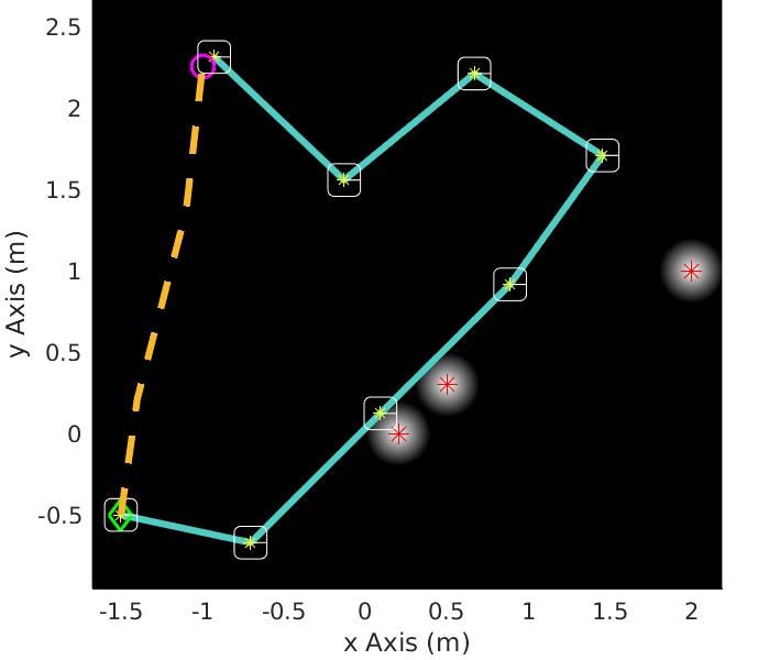
(a) Range-squared, OG-Based

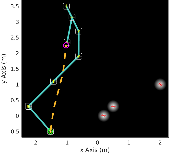
(b) Range-squared, Cov-Based

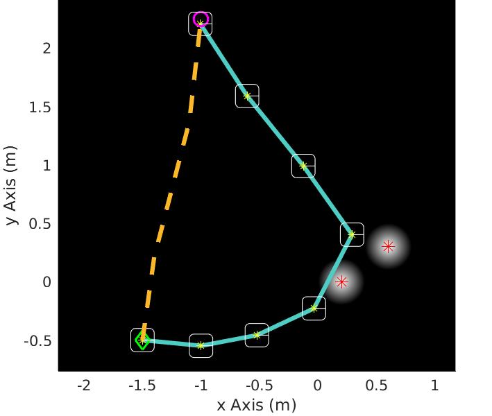
(c) Range, OG-Based

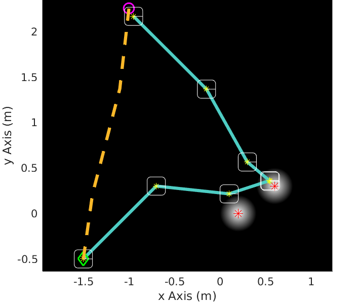
(d) Range, Cov-Based

Figure 1: Simulation results for the planning problem 2 based on the condition number of the OG for range-squared and range observation models in (a) and (c), and the planning problem 3 using the trace of the covariance for range-squared and range observation models in (b) and (d), respectively. The information sources are located in the centers of the light areas. The dashed orange line represents the initial trajectory, while the solid cyan line shows the optimized trajectory.

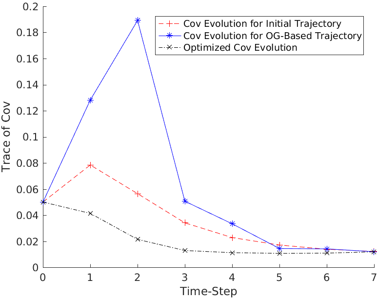
(a) Range-squared

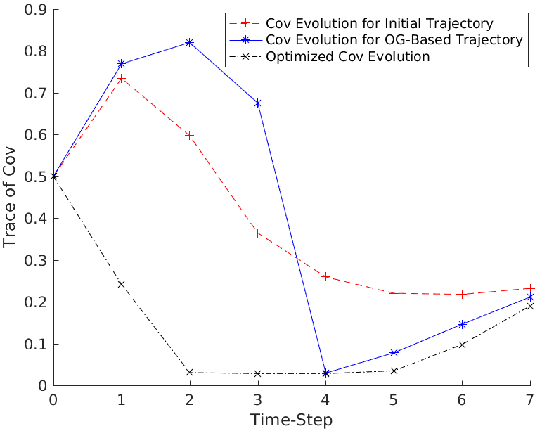
(b) Range

Figure 2: Evolution of the trace of the covariance along the trajectory for the initial trajectory, optimization based on the OG measure, and optimization based on the covariance measure of the trajectories in Fig. 1.

IV-A Range-Squared-Only Observations

Figures 1a and 1b show the results of the simulations for the range-squared-only observation model using the condition number of the OG and the trace of the covariance along the trajectory as the cost function, respectively. Information sources are at $(0.2,0)^{T}$, $(0.5,0.3)^{T}$, and $(2,1)^{T}$, and

$$\boldsymbol{\Sigma}_{\mathbf{x}_{0}}=\begin{pmatrix}0.025&0.002\\ 0.002&0.025\end{pmatrix},\boldsymbol{\Sigma}_{\boldsymbol{\omega}}=\begin{pmatrix}0.3&0.0\\ 0.0&0.1\end{pmatrix},\Sigma_{\nu}=0.1.$$

Figure 2a shows the evolution of the trace of covariance along the trajectories. While it is expected that the trajectory deigned based on the covariance evolution performs better than the other ones, it is surprising to observe that the OG-based trajectory actually under-performs the initial trajectory as well. Even though we have only shown the results of the simulation for the condition number of OG, the interested reader can find a more detailed set of experiments with other measures of the Gramian in a companion technical report [29], which parallel the results provided here. The quantitative result of Fig. 2a, along with the qualitative difference in the trajectories as indicated in Fig. 1, indicate that a measure of the OG is not a reliable measure to optimize in a problem with initial, process and observation uncertainties.

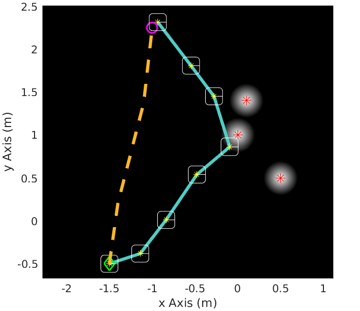
(a) OG-Based Trajectory

(b) Cov-Based Trajectory

Figure 3: Range-only observation model: a) The optimized state trajectory of the planning problem 2 using the condition number of the OG as the cost function, b) The optimized state trajectory of the planning problem 3 using the trace of the covariance as the cost function. The information sources are located in the centers of the light areas. The dashed orange line represents the initial trajectory, while the solid cyan line shows the optimized trajectory.

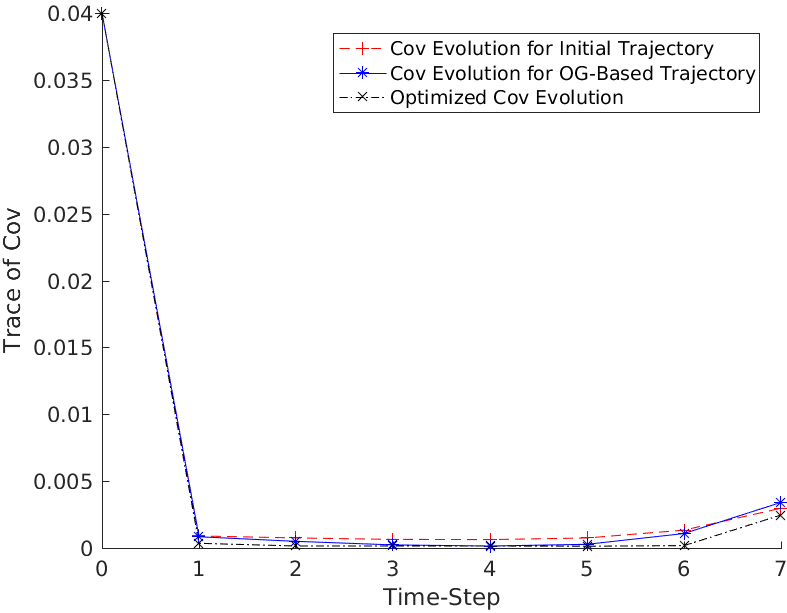
Figure 4: Range observation model. Evolution of the trace of the covariance along the trajectory for the initial trajectory, optimization based on the OG measure, and optimization based on the covariance measure of the trajectories in Fig. 3.

IV-B Range-Only Observations

Figures 1c and 1d show the results of the similar simulations for the range-only observation model with the condition number of the OG and the trace of the covariance as the cost function, respectively. Information sources are at $(0.2,0)^{T}$, and $(0.6,0.3)^{T}$, and

$$\boldsymbol{\Sigma}_{\mathbf{x}_{0}}=\begin{pmatrix}0.25&0\\ 0&0.25\end{pmatrix},\boldsymbol{\Sigma}_{\boldsymbol{\omega}}=\begin{pmatrix}0.1&0\\ 0&1\end{pmatrix},\Sigma_{\nu}=0.015.$$

Figure 2b shows the covariance evolution for the trajectories of this simulation, which resembles the results of Fig. 2a.

IV-C Another Range-Only Scenario

Last, Figs. 3a and 3b show the results of another set of simulations for the range-only observation model using condition number of the OG and the trace of the covariance, respectively. Information sources are located at $(0,1)^{T}$, $(0.5,0.5)^{T}$, and $(0.1,1.4)^{T}$, and

$$\boldsymbol{\Sigma}_{\mathbf{x}_{0}}=\begin{pmatrix}0.02&0\\ 0&0.02\end{pmatrix},\boldsymbol{\Sigma}_{\boldsymbol{\omega}}=\begin{pmatrix}0.1&0\\ 0&0.1\end{pmatrix},\Sigma_{\nu}=0.0001.$$

In this experiment, the reduced noise covariances, particularly the observation covariance, lead to the high quality of measurements from a broad class of trajectories. As a result, the trace of covariance evolution of Fig. 3 indicates only a slight difference between the three trajectories.

Remark: It should be noted that in all the figures, since the state trajectories are softly constrained to reach to the same goal region at the end of the navigation, the covariance evolutions converge to each other towards the end of the trajectories. This is due to the fact that in the Bayesian filtering, the latest observations (which arise from the same region in the state space) carry a higher weight than the prior history. As a result, in comparing the covariance evolutions, the variations in the behavior along the entire trajectory is of concern since a highly certain trajectory can lead to safer navigation, particularly, in a complex environment with obstacles, banned areas or multiple agents.

Remark: Finally, note that the simulation times to solve the optimization problem for all cases are of the same order, which stems from the fact that the computation complexity of both the problems 2 and 3 is $O(Kn_{x}^{3})$ [27].

V Conclusion

In this paper, we have investigated a well-known heuristic employing the observability Gramian in planning under observation uncertainty. We have utilized two common observation models and shown that, in general, the observability Gramian (and the closely-related standard Fisher information matrix) fail to capture many aspects of the models including the initial, process, and observation uncertainties. As a result, based on changes in those models, we showed using analytic and numerical examples that planning based on the observability Gramian can provide trajectories that are very different in terms of the estimation performance from the optimal plans based on the estimation covariance of the problem.

References

- [1] P. S. Maybeck, Stochastic models, estimation, and control. Academic press, 1982, vol. 3, pp. 45–48, 238–241.
- [2] K. Yasuda and R. E. Skelton, “Assigning controllability and observability gramians in feedback control,” Journal of Guidance, Control, and Dynamics, vol. 14, no. 5, pp. 878–885, 1991.
- [3] U. Vaidya, “Observability gramian for nonlinear systems,” in Decision and Control, 2007 46th IEEE Conference on. IEEE, 2007, pp. 3357–3362.
- [4] B. Southall, B. F. Buxton, and J. A. Marchant, “Controllability and observability: Tools for kalman filter design.” in BMVC, 1998, pp. 1–10.
- [5] A. J. Krener and K. Ide, “Measures of unobservability,” in Decision and Control, 2009 held jointly with the 2009 28th Chinese Control Conference. CDC/CCC 2009. Proceedings of the 48th IEEE Conference on. IEEE, 2009, pp. 6401–6406.
- [6] P. R. Kumar and P. P. Varaiya, Stochastic Systems: Estimation, Identification, and Adaptive Control. Englewood Cliffs, NJ: Prentice-Hall, 1986.
- [7] D. Bertsekas, Dynamic Programming and Optimal Control: 3rd Ed. Athena Scientific, 2007.
- [8] M. Rafieisakhaei, A. Tamjidi, S. Chakravorty, and P. Kumar, “Feedback Motion Planning Under Non-Gaussian Uncertainty and Non-Convex State Constraints,” in 2016 IEEE International Conference on Robotics and Automation (ICRA). IEEE, 2016, pp. 4238–4244.
- [9] R. Platt, “Convex receding horizon control in non-gaussian belief space,” in Algorithmic Foundations of Robotics X. Springer, 2013, pp. 443–458.
- [10] R. Platt, R. Tedrake, L. Kaelbling, and T. Lozano-Perez, “Belief space planning assuming maximum likelihood observations,” in Robotics: Science and Systems (RSS), 2010.
- [11] J. Van Den Berg, P. Abbeel, and K. Goldberg, “Lqg-mp: Optimized path planning for robots with motion uncertainty and imperfect state information,” The International Journal of Robotics Research, vol. 30, no. 7, pp. 895–913, 2011.
- [12] D. Georges, “Energy minimization and observability maximization in multi-hop wireless sensor networks,” IFAC Proceedings Volumes, vol. 44, no. 1, pp. 13 918–13 923, 2011.
- [13] B. T. Hinson, “Observability-based guidance and sensor placement,” Ph.D. dissertation, University of Washington, 2014.
- [14] B. T. Hinson, M. K. Binder, and K. A. Morgansen, “Path planning to optimize observability in a planar uniform flow field,” in American Control Conference (ACC), 2013. IEEE, 2013, pp. 1392–1399.
- [15] J. D. Quenzer and K. A. Morgansen, “Observability based control in range-only underwater vehicle localization,” in American Control Conference (ACC), 2014. IEEE, 2014, pp. 4702–4707.
- [16] M. Travers and H. Choset, “Use of the nonlinear observability rank condition for improved parametric estimation,” in Robotics and Automation (ICRA), 2015 IEEE International Conference on. IEEE, 2015, pp. 1029–1035.
- [17] L. DeVries and D. A. Paley, “Wake sensing and estimation for control of autonomous aircraft in formation flight,” Journal of Guidance, Control, and Dynamics, vol. 39, no. 1, pp. 32–41, 2015.
- [18] L. DeVries, S. J. Majumdar, and D. A. Paley, “Observability-based optimization of coordinated sampling trajectories for recursive estimation of a strong, spatially varying flowfield,” Journal of Intelligent & Robotic Systems, vol. 70, no. 1-4, pp. 527–544, 2013.
- [19] A. K. Singh and J. Hahn, “Determining optimal sensor locations for state and parameter estimation for stable nonlinear systems,” Industrial & engineering chemistry research, vol. 44, no. 15, pp. 5645–5659, 2005.
- [20] R. Platt, L. Kaelbling, T. Lozano-Perez, and R. Tedrake, “Non-gaussian belief space planning: Correctness and complexity,” in Robotics and Automation (ICRA), 2012 IEEE International Conference on. IEEE, 2012, pp. 4711–4717.
- [21] P. Tichavsky, C. H. Muravchik, and A. Nehorai, “Posterior cramér-rao bounds for discrete-time nonlinear filtering,” IEEE Transactions on signal processing, vol. 46, no. 5, pp. 1386–1396, 1998.
- [22] N. Thacker and A. Lacey, “Tutorial: The likelihood interpretation of the kalman filter,” TINA Memos: Advanced Applied Statistics, vol. 2, no. 1, pp. 1–11, 1996.
- [23] K. Bastani, B. Barazandeh, and Z. J. Kong, “Fault diagnosis in multistation assembly systems using spatially correlated bayesian learning algorithm,” Journal of Manufacturing Science and Engineering, vol. 140, no. 3, p. 031003, 2018.
- [24] M. Lei, C. Baehr, and P. Del Moral, “Fisher information matrix-based nonlinear system conversion for state estimation,” in Control and Automation (ICCA), 2010 8th IEEE International Conference on. IEEE, 2010, pp. 837–841.
- [25] G. Casella and R. L. Berger, Statistical inference. Duxbury Pacific Grove, CA, 2002, vol. 2.
- [26] M. Rafieisakhaei, S. Chakravorty, and P. R. Kumar, “T-LQG: Closed-Loop Belief Space Planning via Trajectory-Optimized LQG,” in 2017 IEEE International Conference on Robotics and Automation (ICRA). IEEE, 2017, pp. 649–656.
- [27] M. Rafieisakhaei, S. Chakravorty, and P. Kumar, “Belief Space Planning Simplified: Trajectory-optimized LQG (T-LQG),” arXiv preprint arXiv:1608.03013, 2016.
- [28] M. Rafieisakhaei, S. Chakravorty, and P. R. Kumar, “A Near-Optimal Decoupling Principle for Nonlinear Stochastic Systems Arising in Robotic Path Planning and Control,” in 56th IEEE Conference on Decision and Control (CDC). IEEE, 2017.
- [29] M. Rafieisakhaei, S. Chakravorty, and P. R. Kumar, “On the Use of the Observability Gramian for Robotic Path Planning Under Observation Uncertainty,” arXiv preprint arXiv:, 2017.