Spin portal to dark matter.

Abstract

In this work we study the possibility that dark matter fields transform in the $(1,0)\oplus(0,1)$ representation of the Homogeneous Lorentz Group. In an effective theory approach, we study the lowest dimension interacting terms of dark matter with standard model fields, assuming that dark matter fields transform as singlets under the standard model gauge group. There are three dimension-four operators, two of them yielding a Higgs portal to dark matter. The third operator couple the photon and $Z^{0}$ fields to the higher multipoles of dark matter, yielding a spin portal to dark matter. For dark matter ($D$) mass below a half of the $Z^{0}$ mass, the decays $Z^{0}\to\bar{D}D$ and $H\to\bar{D}D$ are kinematically allowed and contribute to the invisible widths of the $Z^{0}$ and $H$. We calculate these decays and use experimental results on these invisible widths to constrain the values of the low energy constants finding in general that effects of the spin portal can be more important that those of the Higgs portal. We calculate the dark matter relic density in our formalism, use the constraints on the low energy constants from the $Z^{0}$ and $H$ invisible widths and compare our results with the measured relic density, finding that dark matter with a $(1,0)\oplus(0,1)$ space-time structure must have a mass $M>43~{}GeV$.

I Introduction.

The elucidation of the nature of dark matter is one of the most important problems in high energy physics Arcadi:2017kky . Although dark matter gravitational effects were noticed during the first half of the last century Zwicky:1933gu and from recent precise measurements of the cosmic background radiation we know that it accounts for around $26\%$ Ade:2015xua of the matter-energy content of the universe, an identification of dark matter properties is still lacking and a lot of experimental effort is presently being pursued in order to directly or indirectly detect dark matter particles, based mainly in the WIMP paradigm Steigman:1984ac . The latter is based on the fact that the proper description of the measured dark matter relic density, $\Omega^{exp}_{DM}h^{2}=0.1186\pm 0.0020$ Ade:2015xua ; Patrignani:2016xqp , requires dark matter to have annihilation cross sections into standard model particles of the order of those produced by the weak interactions.

From the particle physics side, dark matter is a challenging problem since there is no particle in the standard model which can be identified with dark matter and, although some extensions of the standard model such as supersymmetric models or extra-dimension models have candidates to dark matter, no signal for these particles has been found in the exhaustive search for signals of physics beyond the standard model or direct search for dark matter signals carried out at the LHC during the past few years Varnes:2016rzg ; Charlton:2017wfj ; Camporesi:2016fjj .

The problem has also been considered in a model independent way using effective field theories, where the low energy effects of the unknown theory at high energies are considered in a systematic expansion, based on general principles. Effective theories for scalar Silveira:1985rk ; McDonald:1993ex ; Burgess:2000yq ; Kanemura:2010sh ; Andreas:2010dz ; Djouadi:2011aa ; Mambrini:2011ik ; Djouadi:2012zc , fermion Kanemura:2010sh ; Djouadi:2011aa ; LopezHonorez:2012kv ; Djouadi:2012zc or vector Kearney:2016rng ; Bambhaniya:2016cpr ; Cotta:2012nj particles have been proposed, and several experimental direct searches are motivated by these formalisms.

The standard model contains spin 1/2 fermions (quarks and leptons), spin 1 bosons (gauge bosons) and a spin 0 boson (the Higgs particle) with the corresponding fields transforming in the $(\frac{1}{2},0)\oplus(0,\frac{1}{2})$, $(\frac{1}{2},\frac{1}{2})$ and $(0,0)$ representations of the Homogeneous Lorentz Group (HLG) respectively and it is natural that effective theories so far formulated for dark matter consider dark matter transforming in these representations.

Recently, the quantum field theory of spin one massive particles transforming in the $(1,0)\oplus(0,1)$ representation of the HLG (spin-one matter fields), was studied in detail in Napsuciale:2015kua , where the field is described by a six-component spinor, similar to the four-component Dirac spinor describing spin $1/2$ fermions. It was shown there that a consistent quantum field theory of spin-one matter fields requires a constrained dynamics formalism but the constraints are second class and can be solved along Dirac conventional method Dirac:1964 . In order to solve the constraints, however, we need to know the algebraic structure of a covariant basis for the operators acting in the $(1,0)\oplus(0,1)$ representation space, which was previously worked out in Gomez-Avila:2013qaa . This basis naturally contains a chirallity operator, $\chi$, and spin-one matter fields can be decomposed into chiral components transforming in the $(1,0)$ (right) and $(0,1)$ (left) representations. However, the kinetic term in the free Lagrangian is not invariant under independent chiral transformations, therefore spin-one matter fields cannot have linearly realized chiral gauge interactions, hence they cannot have weak interactions. Nonetheless, it is possible to have vector-like interactions like $U(1)_{Y}$ or $SU(3)_{c}$ standard model interactions. In addition, spin-one matter fields can have naively renormalizable self-interactions classified also in Napsuciale:2015kua .

In this work we study the possibility of a $(1,0)\oplus(0,1)$ space-time structure for dark matter fields. Clearly, dark matter with standard model charges would give sizable contributions to precision measurements of standard model observables, thus we assume in this work that dark matter fields transform as singlets of the standard model gauge group.

The paper is organized as follows. In the next section we review the elements of the quantum field theory of spin one matter fields needed for the calculation of the required cross sections. In Section III we discuss the leading terms in the effective field theory. In section IV we study the mass region $M<M_{Z}/2$, calculate the decay width for $Z^{0}\to\bar{D}D$ and $H\to\bar{D}D$ and find the constraints on the low energy constants from the $Z^{0}$ and Higgs invisible widths. Section V contains an analysis of the dark matter relic density in this formalism, when these constraints are taken into account. Finally, we give our conclusions and perspectives in section VI and close with an appendix with the required trace calculations for operators in the $(1,0)\oplus(0,1)$ representation space.

II Quantum field theory for spin-one matter fields: brief review

In the standard model, matter is described by Dirac fermions which transform in the $(1/2,0)\oplus(0,1/2)$ representation of the HLG. Spin-one matter fields are the generalization of Dirac construction to $j=1$, i.e. fields transforming in the $(1,0)\oplus(0,1)$. The basic object is a six-component ‘spinor‘ $\psi(x)$ and the corresponding quantum field theory was studied in Napsuciale:2015kua , taking advantage of the general construction of a covariant basis for $(j,0)\oplus(0,j)$ representation space introduced in Gomez-Avila:2013qaa . For $j=1$ the covariant basis is given by the set of $6\times 6$ matrices $\{\mathbf{1},\chi,S^{\mu\nu},\chi S^{\mu\nu},M^{\mu\nu},C^{\mu\nu\alpha\beta}\}$ where $\chi$ is the chirality operator, $S^{\mu\nu}$, stands for a symmetric traceless ($S\indices{{}^{\mu}_{\mu}}=0$) matrix tensor transforming in the $(1,1)$ representation of the HLG, $M^{\mu\nu}$ are the HLG generators and $C^{\mu\nu\alpha\beta}$ is a matrix tensor transforming in the $(2,0)\oplus(0,2)$ representation of the HLG.

The spin-one matter field is written as

$$\psi(x)=\sum_{\lambda}\int\frac{d^{3}p}{\sqrt{(2\pi)^{3}2E}}[a_{\lambda}(p)\mathcal{U}(p,\lambda)e^{-ip.x}+b^{\dagger}_{\lambda}(p)\mathcal{V}(p,\lambda)e^{ip.x}]$$ (1)

where $\mathcal{U}(p,\lambda)$ ($\mathcal{V}(p,\lambda)$) stands for the particle (antiparticle) solution with polarization $\lambda$ respectively. In contrast with the Dirac case, spin-one matter particle and antiparticle have the same parity. These solutions satisfy

$$\sum_{\lambda}\mathcal{U}\left(p,\lambda\right)\mathcal{\bar{U}}\left(p,\lambda\right)=\frac{S\left(p\right)+M^{2}}{2M^{2}},\qquad\sum_{\lambda}\mathcal{V}\left(p,\lambda\right)\mathcal{\bar{V}}\left(p,\lambda\right)=\frac{S\left(p\right)+M^{2}}{2M^{2}}.$$ (2)

where $S\left(p\right)\equiv S^{\mu\nu}p_{\mu}p_{\nu}$.

The spin-one matter fields free Lagrangian is given by

$$\mathcal{L}=\frac{1}{2}\partial^{\mu}\bar{\psi}(x)(g_{\mu\nu}+S_{\mu\nu})\partial^{\nu}\psi(x)-m^{2}\bar{\psi}(x)\psi(x).$$ (3)

where $\bar{\psi}(x)\equiv(\psi(x))^{\dagger}S^{00}$. The $S^{\mu\nu}$ operators satisfy the following anti-commutation relations

$$\{S^{\mu\nu},S^{\alpha\beta}\}=\frac{4}{3}\left(g^{\mu\alpha}g^{\nu\beta}+g^{\nu\alpha}g^{\mu\beta}-\frac{1}{2}g^{\mu\nu}g^{\alpha\beta}\right)-\frac{1}{6}\left(C^{\mu\alpha\nu\beta}+C^{\mu\beta\nu\alpha}\right).$$ (4)

Further algebraic relations of the operators in the covariant basis and the connection with the traces needed for the calculations in this work are deferred to an appendix. The propagator for spin-one matter particles is given by

$$i\pi(p)=i\frac{S(p)-p^{2}+2M^{2}}{2M^{2}(p^{2}-M^{2}+i\varepsilon)}.$$ (5)

An important outcome of this formalism is that the free field Lagrangian can be decomposed in terms of the chiral components as

$$\mathcal{L}=\frac{1}{2}\partial^{\mu}\overline{\psi_{R}}\partial_{\mu}\psi_{L}+\frac{1}{2}\partial^{\mu}\overline{\psi_{R}}S_{\mu\nu}\partial_{\nu}\psi_{R}-m^{2}\overline{\psi_{R}}\psi_{L}+R\leftrightarrow L,$$ (6)

where

$$\psi_{R}=\frac{1}{2}\left(1+\chi\right)\psi,\qquad\psi_{L}=\frac{1}{2}\left(1-\chi\right)\psi.$$ (7)

The right (left) field $\psi_{R}$ ($\psi_{L}$) transforms in $(1,0)$ ($(0,1)$) representation of the HLG. Notice that in the massless case, the kinetic term couples right and left components, hence it is not invariant under independent chiral transformations. Therefore, spin-one matter fields cannot have chiral gauge interactions, although they admit vector gauge interactions. Concerning the standard model interactions, spin-one matter fields can have only $U(1)_{Y}$ or $SU(3)_{C}$ gauge interactions but not $SU(2)_{L}$ interactions, or simply be standard model singlets. This result motivate us to explore the possibility that dark matter be described by spin-one matter fields and we start with the simplest and most likely possibility: spin-one dark matter fields transforming as singlets under the standard model gauge group.

III Dark matter as spin-one matter fields: effective theory.

If we consider dark matter as spin-one matter fields (spin-one dark matter fields in the following) transforming as singlets under the standard model group, dark matter does not feel the standard model charges. On the other side, if we have more than one dark matter field, dark matter can have gauge interactions with its own (vector-like) dark gauge group. In the following we will assume a simple $U(1)_{D}$ structure for the dark gauge group, but the generalization of our results to $SU(N)_{D}$ is straightforward. We remark that the only effect of this dark gauge structure in this work is to provide to dark matter particles with dark charges distinguishing particles from anti-particles and preventing the direct decay of a dark matter particle into standard model ones.

At high energies, the standard model and dark sectors couple in a yet unknown way but the low energy effects of such theory can be classified in an expansion in derivatives of the fields. Each term in this expansion has a low energy constant and the importance at low energies of each term depends on the dimension of the corresponding operator, in such a way that the most important effects are given by the lowest dimension operators.

The Lagrangian must be a complete scalar operator and if dark matter fields are standard model singlets (and standard model fields are singlets of the dark gauge group) the only possibility to have a scalar interacting Lagrangian is that it be composed of products of singlet operators on both sides. The construction of the lowest dimension interacting operators in this case, requires to classify the singlet operators in both sectors. The most general form of this interaction is

$$\mathcal{L}_{int}=\sum_{n}\frac{1}{\Lambda^{n-4}}\mathcal{O}_{SM}\mathcal{O}_{DM}$$ (8)

where $\Lambda$ is an energy scale compensating the dimension $n$ of the product of the standard model singlet operators $\mathcal{O}_{SM}$ constructed with standard model fields and $\mathcal{O}_{DM}$ made of spin-one dark matter fields.

It is easy to convince one-self that the lowest dimension standard model singlet operators are $\tilde{\phi}\phi$ and $B_{\mu\nu}$, where $\phi$ stands for the standard model Higgs doublet and $B_{\mu\nu}$ denotes the $U(1)_{Y}$ stress tensor. Indeed, $\tilde{\phi}\phi$ is simply the singlet of the $\mathbf{2}\otimes\mathbf{2}$ product of $SU(2)_{L}$ ( and also a singlet under $SU(3)$ and $U(1)_{Y}$), while in general under $SU(N)$ gauge transformations $U(x)$, the stress (matrix) tensor operator transforms as

$$F^{\mu\nu}\to U(x)F^{\mu\nu}U^{-1}(x),$$ (9)

being strictly invariant only in the $U(1)$ case, thus, in the standard model, the $U(1)_{Y}$ stress tensor $B_{\mu\nu}$ is a singlet under the standard model gauge group. Singlet operators made of fermion fields or other combinations can also be constructed but they are higher dimension.

For spin-one matter fields with a dark gauge group $U(1)_{D}$ , the lowest dimension operators transforming as standard model and dark gauge group singlets are of the form $\bar{\psi}O\psi$ where $O$ is one of the $36$ matrix operators in the covariant basis $\{\mathbf{1},\chi,S^{\mu\nu},\chi S^{\mu\nu},M^{\mu\nu},C^{\mu\nu\alpha\beta}\}$. These operators are dimension two and using the symmetry properties of $S^{\mu\nu}$ and $C^{\mu\nu\alpha\beta}$ it is easy to show that the leading interacting terms in the effective theory are given by

$$\mathcal{L}_{int}=\bar{\psi}(g_{s}\mathbf{1}+ig_{p}\chi)\psi\tilde{\phi}\phi+g_{t}\bar{\psi}M_{\mu\nu}\psi B^{\mu\nu},$$ (10)

with low energy constants $g_{s}$, $g_{p}$ and $g_{t}$. There is an effective Higgs portal to dark matter interactions with standard model particles given by the first two terms, the second one violating parity. The third term is an effective interaction coupling dark matter to the photon and the $Z^{0}$ boson. Notice however that this interaction does not involve the weak charges (operators are standard model singlets), but proceeds through the coupling of the photon and $Z^{0}$ fields to the higher multipoles (magnetic dipole moment and electric quadrupole moment) of the dark matter, thus we name it spin portal to dark matter. In addition to the interactions in Eq.(10) we have the dimension four self-interactions described in Napsuciale:2015kua which are not relevant for the purposes of this paper.

In unitary gauge for the standard model fields, after spontaneous symmetry breaking and diagonalizing the gauge boson sector we get the following Lagrangian

$$\mathcal{L}_{int}=\frac{1}{2}\bar{\psi}(g_{s}\mathbf{1}+ig_{p}\chi)\psi\left(H+v\right)^{2}+g_{t}\cos\theta_{W}\bar{\psi}M_{\mu\nu}\psi F^{\mu\nu}-g_{t}\sin\theta_{W}\bar{\psi}M_{\mu\nu}\psi Z^{\mu\nu},$$ (11)

where $H$ stands for the Higgs field, $v$ denotes the Higgs vacuum expectation value and $F^{\mu\nu},Z^{\mu\nu}$ are the electromagnetic and $Z^{0}$ stress tensors respectively. The Feynman rules arising from the Lagrangian in Eq. (11) are given in Fig. 1.

Figure 1: Feynman rules from the leading terms in the effective theory.

IV Dark matter with a mass $M<M_{Z}/2$ : $Z^{0}\to\bar{D}D$ and $H\to\bar{D}D$ decays.

The Lagrangian in Eq.(11) induces transitions between the standard model and dark sectors. Annihilation of dark matter into standard model particles such as $\bar{D}D\to\bar{f}f,\gamma\gamma,W^{+}W^{-},Z^{0}Z^{0},HH,Z^{0}\gamma,H\gamma,Z^{0}H$ which could be important in the description of dark matter relic density are induced by these interactions under appropriate kinematical conditions. Also, for dark matter mass below half the $Z^{0}$ mass ($M<M_{Z}/2$), the decays $Z^{0}\to\bar{D}D$ and $H\to\bar{D}D$ are kinematically permitted and contribute to the invisible $Z^{0}$ and $H$ widths respectively. In this work we consider this mass region and work out the predictions of the formalism for the dark matter relic density.

A straightforward calculation yields the following invariant amplitude for the $Z^{0}(k,\epsilon)\to D(p_{1})\bar{D}(p_{2})$ decay

$$-i\mathcal{M}=2g_{t}S_{W}\bar{\mathcal{U}}(p_{1},\lambda_{1})M^{\mu\nu}k_{\nu}\mathcal{V}(p_{2},\lambda_{2}))\epsilon_{\mu}(k),$$ (12)

where $S_{W}=\sin\theta_{W}$. The calculation of the average squared amplitude can be reduced to a trace of products of operators in the covariant basis of $(1,0)\oplus(0,1)$ representation space, in a procedure similar to conventional calculations with Dirac fermions. We obtain

$$|\bar{\mathcal{M}}|^{2}=\frac{4}{3}g^{2}_{t}S^{2}_{W}Tr\left[\frac{S(p_{1})+M^{2}}{2M^{2}}M^{\mu\nu}\frac{S(p_{2})+M^{2}}{2M^{2}}M^{\alpha\beta}\right]k_{\nu}k_{\beta}(-g_{\mu\alpha}+\frac{k_{\mu}k_{\alpha}}{M^{2}_{Z}}).$$ (13)

The trace-ology of matrices in $(1,0)\oplus(0,1)$ space is deferred to an appendix. Using results in the appendix we obtain the corresponding decay width as

$$\Gamma(Z^{0}\to\bar{D}D)=\frac{g_{t}^{2}S^{2}_{W}}{24\pi M^{4}}(M_{Z}^{2}-4M^{2})^{3/2}(M_{Z}^{2}+2M^{2}).$$ (14)

The invisible width $\Gamma^{inv}_{exp}(Z)=499.0\pm 1.5~{}MeV$ reported by the Particle Data Group Patrignani:2016xqp , includes the decay to $\nu\bar{\nu}$. We use the SM prediction for the latter

$$\Gamma_{SM}(Z^{0}\to\bar{\nu}\nu)\equiv\sum_{i}\Gamma_{SM}(Z^{0}\to\bar{\nu}_{i}\nu_{i})=\sum_{i,\alpha}U_{i\alpha}^{2}\frac{M^{2}_{Z}}{24\pi v^{2}}\sqrt{M^{2}_{Z}-4m^{2}_{\nu_{i}}}=\frac{M^{3}_{Z}}{8\pi v^{2}}=\frac{\sqrt{2}G_{F}M^{3}_{Z}}{8\pi}.$$ (15)

where in the last step we neglected the neutrino masses and used the unitarity of the PMNS matrix elements. The Particle Data Group report the value $M_{Z}=91.1876\pm 0.0021~{}GeV$ while the $\mu-Lan$ collaboration reported the most precise measurement of the Fermi constant as $G_{F}=1.1663788(6)\times 10^{-5}GeV^{-2}$ Webber:2010zf . Using these values we get

$$\Gamma_{SM}(Z^{0}\to\bar{\nu}\nu)=497.64\pm 0.03~{}MeV.$$ (16)

Subtracting this quantity from the PDG reported value for the invisible width we get the constraint $\Gamma(Z\to\bar{D}D)<\Gamma^{inv}_{Z}\equiv\Gamma^{inv}_{exp}(Z)-\Gamma_{SM}(Z\to\bar{\nu}\nu)=1.4\pm 1.5~{}MeV$. This width depends on the coupling $g_{t}$ and the dark matter mass $M$, hence the invisible $Z^{0}$ width constrain these parameters to the region shown in Fig. 2.

Similar calculations for the $H\to\bar{D}D$ decay yield the following decay width

$$\Gamma(H\to\bar{D}D)=\frac{v^{2}}{32\pi M^{2}_{H}M^{4}}\sqrt{M_{H}^{2}-4M^{2}}\left[g_{s}^{2}\left(M_{H}^{2}\left(M_{H}^{2}-4M^{2}\right)+6M^{4}\right)+g_{p}^{2}M_{H}^{2}\left(M_{H}^{2}-4M^{2}\right)\right],$$ (17)

The $H\to\bar{D}D$ width depends on the unknown $g_{s}$, $g_{p}$ couplings and on the dark matter mass. This channel contributes to the invisible Higgs width which has been recently reported in Patrignani:2016xqp ; Khachatryan:2016whc as $\Gamma^{inv}_{H}=1.14\pm 0.04~{}MeV$. In this case, the contribution of the $\nu\bar{\nu}$ channel is negligible. The constraints on $g_{s},g_{p}$ arising from the $\Gamma(H\to\bar{D}D)<\Gamma^{inv}_{H}$ condition are also shown in Fig. 2. The solid lines correspond to the central values and the shadow regions to the one sigma regions. We conclude from this plot that the coupling of the spin portal $g_{t}$ in general can be larger than those of the Higgs portal $g_{s}$ or $g_{p}$, by at least one order of magnitude.

Figure 2: Parameter space for $g_{t},g_{s}$ and $g_{p}$ consistent $\Gamma(Z\to\bar{D}D)<\Gamma^{inv}_{Z}=1.4\pm 1.5~{}MeV$ and $\Gamma(H\to\bar{D}D)<\Gamma^{inv}_{H}=1.14\pm 0.04~{}MeV$ for $M<M_{Z}/2$. Solid lines correspond to the central values of the invisible decay widths.

V Dark matter relic density.

V.1 Boltzman equation.

The evolution of the dark matter comoving number density $n_{D}(T)$ is described by the Boltzmann equation Dodelson:2003ft

$$\frac{dY}{dx}=-\frac{\lambda(x)}{x^{2}}(Y^{2}-Y^{2}_{eq}),$$ (18)

where $x=M/T$, $Y(x)=n_{D}(x)/T^{3}$ and

$$\lambda(x)\equiv\frac{M^{3}\langle\sigma v_{r}\rangle}{H(M)}.$$ (19)

Here, $H(M)=M^{2}\sqrt{\frac{8\pi^{3}G_{N}g_{*}(M)}{90}}$ stands for the Hubble parameter at the dark mass scale, $M$, with $G_{N}=6.70861(31)\times 10^{-39}GeV^{-2}$ denoting the Newton gravitational constant Patrignani:2016xqp , $g^{*}(M)$ standing for the relativistic effective degrees of freedom at $T=M$ in the thermal bath and

$$Y_{eq}(x)=\frac{n_{D}^{eq}}{T^{3}}=\frac{g_{D}}{T^{3}}\int\frac{d^{3}p}{(2\pi)^{3}}\frac{1}{e^{\frac{E}{T}}-1}=\frac{3}{2\pi^{2}}\int_{x}^{\infty}\frac{u\sqrt{u^{2}-x^{2}}du}{e^{u}-1}\approx\frac{3}{2\pi^{2}}\int_{x}^{\infty}e^{-u}u\sqrt{u^{2}-x^{2}}du.$$ (20)

The thermal average $\langle\sigma v_{r}\rangle$ includes all channels for the annihilation $D(p_{1})\bar{D}(p_{2})\to X(p_{3})Y(p_{4})$ of dark matter into standard model particles $X,Y$ in the thermal bath and it is given by

$$\langle\sigma v_{r}\rangle=\frac{1}{n_{D}^{eq}n_{\bar{D}}^{eq}}\int\frac{g_{D}d^{3}p_{1}}{(2\pi)^{2}}e^{-E_{1}/T}\int\frac{g_{\bar{D}}d^{3}p_{2}}{(2\pi)^{2}}e^{-E_{2}/T}\sigma v_{r},$$ (21)

where $g_{D}$ ($g_{\bar{D}}$)denotes the number of internal d.o.f of the dark matter particle (antiparticle), $v_{r}$ stands for the dark matter particle-antiparticle relative velocity and $\sigma$ is the conventional cross section for the $D(p_{1})\bar{D}(p_{2})\to X(p_{3})Y(p_{4})$ process.

A qualitative analysis of the solution of Eq. (18) assuming the freezing of dark matter at some temperature which would explain dark matter relic density, shows that dark matter must be non-relativistic at the time of its decoupling from the cosmic plasma Dodelson:2003ft . This is consistent with data on dark matter relic density extracted from precision measurement of the cosmic background radiation Ade:2015xua ; Patrignani:2016xqp . In this case, it is a good approximation to perform a non-relativistic expansion of $\langle\sigma v_{r}\rangle$ keeping only the leading terms in the expansion in powers of $v_{r}<<1$. This expansion requires the calculation of the flux for dark matter particles in the thermal bath, which can be written as Gondolo:1990dk ; Cannoni:2016hro

$$F=4\sqrt{(p_{1}\cdot p_{2})^{2}-M^{4}}=2(s-M^{2})v_{r}$$ (22)

where $v_{r}$ is related to $s$ as

$$s=2M^{2}\left(1+\frac{1}{\sqrt{1-v^{2}_{r}}}\right)=4M^{2}+M^{2}v^{2}_{r}+....$$ (23)

In the last step we performed the non-relativistic expansion for $v_{r}<<1$. The cross section $\sigma$ is a function of $s$ thus using Eq.(22) the leading terms in the expansion are

$$\sigma v_{r}=a+bv^{2}_{r},$$ (24)

and performing the thermal average we obtain

$$\langle\sigma v_{r}\rangle=a+\frac{6b}{x}.$$ (25)

For non-relativistic dark matter with $M<M_{Z}/2$, the kinematically allowed channels are $\bar{D}D\to\bar{f}f$ for fermions with $m_{f}<M$ and $\bar{D}D\to\gamma\gamma$. In the following we calculate the corresponding cross sections in our formalism, perform the non-relativistic expansion and work out the predictions for the $a,b$ coefficients.

V.2 Annihilation of dark matter into a fermion-antifermion pair.

There are three contributions to the process $D(p_{1})\bar{D}(p_{2})\rightarrow f(p_{3})\bar{f}(p_{4})$ shown in Fig. 3.

Figure 3: Feynman diagrams for $\bar{D}D\to\bar{f}f$.

The corresponding amplitudes are given by

$$-i\mathcal{M}_{H} = i\frac{m_{f}}{s-M_{H}^{2}}\bar{u}\left(p_{3}\right)v\left(p_{4}\right)\mathcal{\bar{V}}\left(p_{2}\right)\left(g_{s}I+ig_{p}\chi\right)\mathcal{U}\left(p_{1}\right),$$

$$-i\mathcal{M}_{\gamma} = -\frac{4Q_{f}g_{t}M_{W}S_{W}C_{W}}{vs}\bar{u}\left(p_{3}\right)\gamma^{\mu}v\left(p_{4}\right)\mathcal{\bar{V}}\left(p_{2}\right)M_{\mu\beta}\left(p_{1}+p_{2}\right)^{\beta}\mathcal{U}\left(p_{1}\right),$$ (26)

$$-i\mathcal{M}_{Z} = \frac{g_{t}M_{Z}S_{W}}{v(s-M_{Z}^{2})}\bar{u}\left(p_{3}\right)\gamma^{\mu}\left(A_{f}+B_{f}\gamma_{5}\right)v\left(p_{4}\right)\mathcal{\bar{V}}\left(p_{2}\right)M_{\mu\beta}\left(p_{1}+p_{2}\right){\beta}\mathcal{U}\left(p_{1}\right).$$

Here, $C_{W}=Cos\theta_{W}$, $Q_{f}$ stands for the fermion charge in units of the proton charge $e$, while the $A_{f},B_{f}$ factors are related to the corresponding fermion weak isospin $T^{f}_{3}$ as

$$A_{f}=2T^{f}_{3}-4Q_{f}S^{2}_{W},\qquad B_{f}=-2T^{f}_{3}.$$ (27)

A straightforward calculation yields the following average squared amplitude in terms of the Mandelstam variables

$$\left|\overline{\mathcal{M}_{\bar{f}f}}\right|^{2}= -\frac{g_{t}^{2}M_{Z}^{2}S_{W}^{2}}{9M^{4}v^{2}\left(s-M_{Z}^{2}\right)^{2}}\left[4M^{2}\left(A_{f}^{2}+B_{f}^{2}\right)m_{f}^{4}\left(4M^{2}-s\right)\right.$$

$$+4m_{f}^{2}\left.\left(4M^{2}-s\right)\left(A_{f}^{2}M^{2}\left(2M^{2}+s-t-u\right)+B_{f}^{2}\left(2M^{4}-M^{2}(s+t+u)-s^{2}\right)\right)\right.$$

$$+\left.\left(A_{f}^{2}+B_{f}^{2}\right)\left(16M^{8}-4M^{6}(s+4(t+u))+4M^{4}(t+u)(s+t+u)+M^{2}\left(4s^{3}-2s\left(t^{2}+u^{2}\right)\right)+s^{2}\left((t-u)^{2}-s^{2}\right)\right)\right]$$

$$+\frac{8A_{f}C_{W}Q_{f}g_{t}^{2}M_{W}M_{Z}S_{W}^{2}}{9M^{4}sv^{2}\left(s-M_{Z}^{2}\right)}\left[4M^{2}m_{f}^{2}\left(4M^{2}-s\right)\left(2M^{2}+s-t-u\right)+4m_{f}^{4}\left(4M^{4}-M^{2}s\right)+16M^{8}\right.$$

$$\left.-4M^{6}(s+4(t+u))+4M^{4}(t+u)(s+t+u)+M^{2}\left(4s^{3}-2s\left(t^{2}+u^{2}\right)\right)+s^{2}\left((t-u)^{2}-s^{2}\right)\right]$$

$$+\frac{A_{f}m_{f}^{2}g_{s}g_{t}M_{Z}S_{W}}{9M^{4}v\left(s-M_{H}^{2}\right)\left(s-M_{Z}^{2}\right)}s\left(2M^{2}-s\right)(t-u)$$

$$-\frac{16C_{W}m_{f}^{2}Q_{f}g_{s}g_{t}M_{W}S_{W}}{9M^{4}v\left(s-m_{H}^{2}\right)}\left(2M^{2}-s\right)(t-u)$$

$$-\frac{16C_{W}^{2}Q_{f}^{2}g_{t}^{2}M_{W}^{2}S_{W}^{2}}{9M^{4}s^{2}v^{2}}\left[4M^{2}m_{f}^{2}\left(4M^{2}-s\right)\left(2M^{2}+s-t-u\right)+4m_{f}^{4}\left(4M^{4}-M^{2}s\right)\right.$$

$$\left.+16M^{8}-4M^{6}(s+4(t+u))+4M^{4}(t+u)(s+t+u)+M^{2}\left(4s^{3}-2s\left(t^{2}+u^{2}\right)\right)+s^{2}\left((t-u)^{2}-s^{2}\right)\right]$$

$$+\frac{m_{f}^{2}}{9M^{4}\left(s-M_{H}^{2}\right)^{2}}\left(s-4m_{f}^{2}\right)\left[g_{p}^{2}s\left(s-4M^{2}\right)+g_{s}^{2}\left(6M^{4}-4M^{2}s+s^{2}\right)\right].$$ (28)

Integrating the final state phase space finally we obtain the following cross section for $\bar{D}D\to\bar{f}f$ where we can easily identify the individual contributions from $H,Z^{0}$ and $\gamma$ exchange as well as the $Z^{0}-\gamma$ interference:

$$\sigma_{\bar{f}f}(s) =\frac{1}{72\pi M^{4}\sqrt{s}}\frac{\sqrt{s-4m_{f}^{2}}}{F}\left[\frac{m_{f}^{2}\left(s-4m_{f}^{2}\right)\left(g_{p}^{2}s\left(s-4M^{2}\right)+g_{s}^{2}\left(6M^{4}-4M^{2}s+s^{2}\right)\right)}{\left(s-M_{H}^{2}\right)^{2}}\right.$$

$$\left.+\frac{2g_{t}^{2}M_{Z}^{2}S_{W}^{2}s\left(s-4M^{2}\right)\left(2M^{2}+s\right)\left(2\left(A_{f}^{2}-2B_{f}^{2}\right)m_{f}^{2}+s\left(A_{f}^{2}+B_{f}^{2}\right)\right)}{3v^{2}\left(s-M_{Z}^{2}\right){}^{2}}\right.$$

$$\left.+\frac{32C_{W}^{2}Q_{f}^{2}g_{t}^{2}M_{W}^{2}S_{W}^{2}\left(s-4M^{2}\right)\left(2M^{2}+s\right)\left(2m_{f}^{2}+s\right)}{3v^{2}s}\right.$$

$$\left.-\frac{16A_{f}C_{W}Q_{f}g_{t}^{2}M_{W}M_{Z}S_{W}^{2}\left(s-4M^{2}\right)\left(2M^{2}+s\right)\left(2m_{f}^{2}+s\right)}{3v^{2}\left(s-M_{Z}^{2}\right)}\right].$$ (29)

Notice that the $H-Z$ and $H-\gamma$ interferences vanish after integration of phase space.

V.3 Dark matter annihilation into two photons

This process is induced by the $t$ and $u$ channel dark matter exchange shown in Fig. 4. The corresponding amplitudes are given by

$$-i\mathcal{M}_{t} = i\frac{2g^{2}_{t}C^{2}_{W}}{M^{2}}\bar{V}(p_{2},\lambda_{2})M_{\alpha\beta}\frac{S(p_{1}-p_{3})-t+2M^{2}}{t-M^{2}}M_{\mu\nu}U(p_{1},\lambda_{1})p_{4}^{\alpha}\eta^{\beta}(p_{4})p_{3}^{\mu}\epsilon^{\nu}(p_{3}),$$ (30)

$$-i\mathcal{M}_{u} = i\frac{2g^{2}_{t}C^{2}_{W}}{M^{2}}\bar{V}(p_{2},\lambda_{2})M_{\mu\nu}\frac{S(p_{1}-p_{4})-u+2M^{2}}{u-M^{2}}M_{\alpha\beta}U(p_{1},\lambda_{1})p_{4}^{\alpha}\eta^{\beta}(p_{4})p_{3}^{\mu}\epsilon^{\nu}(p_{3}).$$ (31)

The average squared amplitude is given by

$$|\overline{\mathcal{M}_{\gamma\gamma}}|^{2}=\left(\frac{2g^{2}_{t}C^{2}_{W}}{3M^{2}}\right)^{2}Tr\left[\frac{S(p_{2})+M^{2}}{2M^{2}}T_{\alpha\beta\mu\nu}\frac{S(p_{1})+M^{2}}{2M^{2}}\bar{T}_{\sigma~{}\rho}^{~{}\beta~{}\nu}\right]p_{3}^{\mu}p_{3}^{\rho}p_{4}^{\alpha}p_{4}^{\sigma},$$ (32)

where

$$T_{\alpha\beta\mu\nu} = M_{\alpha\beta}\frac{S(p_{1}-p_{3})-t+2M^{2}}{t-M^{2}}M_{\mu\nu}+M_{\mu\nu}\frac{S(p_{1}-p_{4})-u+2M^{2}}{u-M^{2}}M_{\alpha\beta},$$ (33)

$$\bar{T}_{\alpha\beta\mu\nu} = M_{\mu\nu}\frac{S(p_{1}-p_{3})-t+2M^{2}}{t-M^{2}}M_{\alpha\beta}+M_{\alpha\beta}\frac{S(p_{1}-p_{4})-u+2M^{2}}{u-M^{2}}M_{\mu\nu}.$$ (34)

Figure 4: Feynman diagrams for $\bar{D}D\rightarrow\gamma\gamma$.

A straightforward calculation using the algebraic relations in the appendix yields

$$\overline{|\mathcal{M}_{\gamma\gamma}|^{2}} =\frac{2C_{W}^{4}g_{t}^{4}}{9M^{8}\left(t-M^{2}\right)^{2}\left(u-M^{2}\right)^{2}}\left[6\left(tu\right)^{4}+2\left(tu\right)^{3}\left(-13M^{4}+11M^{2}s+2s^{2}\right)\vskip 3.0pt plus 1.0pt minus 1.0pt\right.$$

$$+\left(tu\right)^{2}\left(42M^{8}-76M^{6}s+33M^{4}s^{2}+4M^{2}s^{3}+2s^{4}\right)\vskip 3.0pt plus 1.0pt minus 1.0pt$$

$$+2M^{2}tu\left(-15M^{10}+43M^{8}s-44M^{6}s^{2}+17M^{4}s^{3}-6M^{2}s^{4}+2s^{5}\right)\vskip 3.0pt plus 1.0pt minus 1.0pt$$

$$+\left.M^{4}\left(8M^{12}-32M^{10}s+51M^{8}s^{2}-40M^{6}s^{3}+25M^{4}s^{4}-12M^{2}s^{5}+2s^{6}\right)\vskip 3.0pt plus 1.0pt minus 1.0pt\right]$$ (35)

Integrating the final state phase space we get the following cross section

$$\sigma_{\gamma\gamma}(s) =\frac{1}{F\sqrt{1-\frac{4M^{2}}{s}}}\frac{C_{W}^{4}g_{t}^{4}}{540\pi M^{8}}\left[120M^{4}\left(4M^{4}-3M^{2}s-2s^{2}\right)\tanh^{-1}\sqrt{1-\frac{4M^{2}}{s}}\right.$$

$$\left.+s\sqrt{1-\frac{4M^{2}}{s}}\left(-10M^{6}+228M^{4}s-99M^{2}s^{2}+43s^{3}\right)\right].$$ (36)

V.4 Dark matter relic density

Expanding the $\bar{D}D\to\bar{f}f$ and $\bar{D}D\to\gamma\gamma$ cross sections we get

$$\sigma v_{r}\equiv\sigma_{\gamma\gamma}v_{r}+\sum_{f}\sigma_{\bar{f}f}v_{r}=a+bv_{r}^{2}$$ (37)

where the sum runs over all the kinematically allowed fermion states ($m_{f}<M$) and

$$a = \frac{29C_{W}^{4}g_{t}^{4}}{18\pi M^{2}}+\sum_{f}\frac{N_{f}g_{s}^{2}m_{f}^{2}\left(M^{2}-m_{f}^{2}\right)^{\frac{3}{2}}}{12\pi M^{3}\left(M_{H}^{2}-4M^{2}\right){}^{2}}$$

$$b = \frac{365C_{W}^{4}g_{t}^{4}}{216\pi M^{2}}+\sum_{f}\frac{N_{f}\sqrt{M^{2}-m_{f}^{2}}}{864\pi M^{5}}\left(\frac{96M^{4}g_{t}^{2}M_{Z}^{2}S_{W}^{2}\left(\left(A_{f}^{2}-2B_{f}^{2}\right)m_{f}^{2}+2M^{2}\left(A_{f}^{2}+B_{f}^{2}\right)\right)}{v^{2}\left(M_{Z}^{2}-4M^{2}\right){}^{2}}\right.$$

$$\left.+\frac{192A_{f}M^{2}C_{W}Q_{f}g_{t}^{2}M_{W}M_{Z}S_{W}^{2}\left(m_{f}^{2}+2M^{2}\right)}{v^{2}\left(M_{Z}^{2}-4M^{2}\right)}+\frac{96C_{W}^{2}Q_{f}^{2}g_{t}^{2}M_{W}^{2}S_{W}^{2}\left(m_{f}^{2}+2M^{2}\right)}{v^{2}}\right.$$

$$\left.-\frac{6M^{2}m_{f}^{2}\left(8g_{p}^{2}\left(4M^{2}-M_{H}^{2}\right)\left(M^{2}-m_{f}^{2}\right)+g_{s}^{2}\left(-8m_{f}^{2}\left(M^{2}-M_{H}^{2}\right)-11M^{2}M_{H}^{2}+20M^{4}\right)\right)}{\left(M_{H}^{2}-4M^{2}\right)^{3}}\right.$$

$$\left.-\frac{9M^{2}m_{f}^{2}g_{s}^{2}\left(4M^{2}-5m_{f}^{2}\right)}{\left(M_{H}^{2}-4M^{2}\right){}^{2}}\right),$$

with $N_{f}=3$ for quarks and $N_{f}=1$ for leptons. We can see in these equations that for the mass region $M<M_{Z}/2$ the Higgs portal contributions are suppressed compared to the spin portal ones by factors $m^{2}_{f}/M^{2}_{H}$.

In Fig. (5) we analize the Higgs and spin portal contributions to $\langle\sigma v_{r}\rangle$ as a function of the couplings for different values of the dark matter mass. In general, we find that Higgs portal contributions are negligible compared to the contributions of the spin portal. Therefore, we will neglect the contribution of the Higgs portal for the calculation of the relic density in the following.

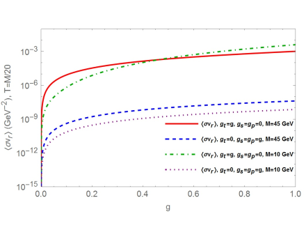
Figure 5: Individual contributions of the spin portal ($g_{t}=g,~{}g_{s}=g_{p}=0$) and the Higgs portal ($g_{t}=0,~{}g_{s}=g_{p}=g$) to $\langle\sigma v_{r}\rangle$. Similar results are obtained in the second case when varying independently $g_{s}$ or $g_{p}$.

Using Eqs. (25,V.4), we numerically solve Boltzman equation (18) for different values of $g_{t}$ and $M$, matching the solution $Y(x)$ with the equilibrium solution $Y_{eq}(x)$ in Eq.(20) at high temperatures, i.e., in the relativistic regime $x<<1$. In Fig.(6) we show the solutions for some specific values of $g_{t}$ and $M$. Clearly, at some temprature $T_{f}$ the solution $Y(x)$ departs from the equilibrium solution $Y_{eq}(x)$ and dark matter decouples from the cosmic plasma in the non-relativistic regime, $x>>1$.

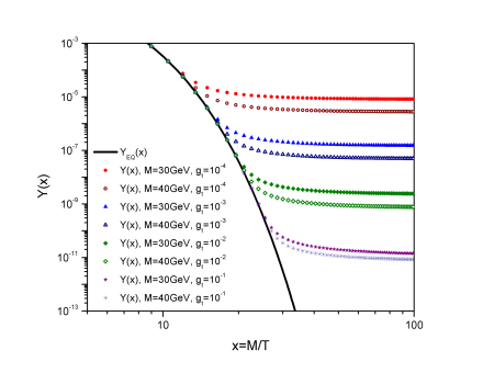
Figure 6: Solution of the Boltzman equation for different values of $M$ and $g_{t}$ showing that dark matter decouples in the non-relativistic regime. The solid line corresponds to $Y_{eq}(x)$.

In order to find the dark matter relic density we need to calculate $Y$ for the present temperature $T_{0}$. This can be done from the numeric solution to Boltzman equation for specific values of $g_{t}$ and $M$ scanning the parameter space consistent with the measured relic density. It is however more illustrative to follow the semi-analytic procedure that takes advance of the freezing mechanism. For $x>x_{f}$ we have $Y(x)>>Y_{eq}(x)$ an we can find an approximate solution neglecting $Y_{eq}(x)$ in the r.h.s of Eq.(18) and integrating from $T_{f}$ to a given temperature $T$, which for our purposes we take as the present temperature $T_{0}$, to obtain

$$\frac{1}{Y(x_{0})}=\frac{1}{Y(x_{f})}+\sqrt{\frac{90}{8\pi^{3}G_{N}}}M\int_{x_{f}}^{x_{0}}\frac{\langle\sigma v\rangle}{\sqrt{g_{*}(x)}x^{2}}dx.$$ (39)

The relic dark matter density is given by

$$\Omega_{DM}=\frac{\rho_{DM}(x_{0})}{\rho_{c}}=\frac{(n_{D}(x_{0})+n_{\bar{D}}(x_{0}))M}{\rho_{c}}=\frac{2n_{D}(x_{0})M}{\rho_{c}}=\frac{2MY(x_{0})T^{3}_{0}}{\rho_{c}},$$ (40)

where we used $n_{\bar{D}}=n_{D}$ and $\rho_{c}=\frac{3H^{2}_{0}}{8\pi G_{N}}=1.05371(5)\times 10^{-5}h^{2}GeV/cm^{3}=8.09619(38)\times 10^{-47}h^{2}GeV^{4}$ is the critical density Patrignani:2016xqp . Neglecting the term $Y(x_{f})^{-1}$ in Eq. (39) which turns out to be small compared with the second term we get

$$\Omega_{DM}h^{2}=\frac{2T^{3}_{0}h^{2}}{\rho_{c}}\sqrt{\frac{8\pi^{3}G_{N}}{90}}\left(\int_{x_{f}}^{x_{0}}\frac{\langle\sigma v\rangle}{\sqrt{g_{*}(x)}x^{2}}dx\right)^{-1}=4.337\times 10^{-11}GeV^{-2}\left(\int_{x_{f}}^{x_{0}}\frac{\langle\sigma v\rangle}{\sqrt{g_{*}(x)}x^{2}}dx\right)^{-1}$$ (41)

where we used $T_{0}=2.7255(6)K=2.34865(52)\times 10^{-13}GeV$ Patrignani:2016xqp . Notice that the r.h.s. of this equation depends on $g_{t}$ and $M$. For a given $M$ we can find the values of $g_{t}$ consistent with the measured value of the relic density. In our calculations we use the complete function $g_{*}(x)$ but our results are quite similar if we use the average over the range of energies considered, $\bar{g}_{*}=33$.

The freezing value $x_{f}$ can be found from the condition that the annihilation rate equals the expansion rate of the universe

$$n_{eq}(x_{f})\langle\sigma v\rangle(x_{f})=H(x_{f}),$$ (42)

which using the non-relativistic form for $n_{eq}(x)$ and Eq. (25) leads to

$$\left(a+\frac{6b}{x_{f}}\right)\sqrt{x_{f}}e^{-x_{f}}=\frac{(2\pi)^{3}}{3M}\sqrt{\frac{G_{N}g^{*}(x_{f})}{90}}.$$ (43)

The value of $x_{f}$ depends also on $g_{t}$ and $M$, so we have two conditions, Eqs. (41,43), for the three variables $x_{f},g_{t},M$ which are solved numerically to obtain the set of values $g_{t}(M)$ consistent with the measured dark matter relic density. The set of values $g_{t}(M)$ is shown in Figure 7. We checked also that these solutions are consistent with the approximations used, i.e. that decoupling occurs when dark matter is non-relativistic. The values of $x_{f}$ corresponding to $g_{t}(M)$ lie in the range $23.8<x_{f}<27.9$, thus $x_{f}>>1$. Finally, we directly calculate $Y(x)$ from the numeric general solution of the Boltzman equation for the set of values $g_{t}(M)$, matching the solution with $Y_{eq}(x)$ for $x<<x_{f}$ finding indeed that $1/Y(x_{f})$ is small compared to $1/Y(x_{0})$ in Eq.(39).

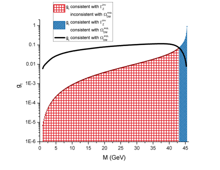
Figure 7: Values of $g_{t}$ and $M$ consistent with the measured dark matter relic density, $\Omega^{exp}_{DM}h^{2}=0.1186\pm 0.0020$ (solid line). The shadowed region denotes the values consistent with the constraint $\Gamma(Z^{0}\to\bar{D}D)<\Gamma^{inv}_{Z}=1.4\pm 1.5~{}MeV$. These constraints exclude masses below $43~{}GeV$ for dark matter with a $(1,0)\oplus(0,1)$ space-time structure.

Our results are summarized in Figure 7, where it is clear that taking into account constraints from the data on the $Z^{0}$ invisible width and from the measured dark matter relic density, dark matter with a $(1,0)\oplus(0,1)$ space-time structure must have a mass $M>43~{}GeV$.

VI Conclusions and perspectives

Effective theories for the interaction of dark matter with standard model fields has been done mainly assuming space-time structures for dark matter similar to those of the standard model fields, i.e., dark matter fields transforming in the $(0,0)$, $(\frac{1}{2},0)\oplus(0,\frac{1}{2})$ or $(\frac{1}{2},\frac{1}{2})$ representations of the HLG.

In this work we study the possibility of a $(1,0)\oplus(0,1)$ space-time structure for dark matter fields. Assuming that dark matter fields are standard model singlets, we find three lowest order terms which are dimension-four in the corresponding effective theory. Two of them couple the Higgs to dark matter and the third one couples the photon and $Z^{0}$ fields to higher multipoles of the spin-one dark matter fields, yielding a spin portal to dark matter.

We start the study of the phenomenology derived from our proposal considering dark matter mass $M<M_{Z}/2$, in whose case the $H\to\bar{D}D$ and $Z^{0}\to\bar{D}D$ are kinematically permitted and contribute to the Higgs and $Z^{0}$ invisible decay widths. We use experimental results on these widths to put upper limits to the corresponding low energy constants. In general we find stringent constraints for the couplings of the Higgs portal: $g_{s},g_{p}\leq 10^{-3}$ and less stringent constraints on the spin portal coupling $g_{t}$.

For dark matter mass in this region, non-relativistic dark matter can annihilate into a photon pair or into a fermion-anti-fermion pair if $M>m_{f}$. We calculate these processes in our formalism and use them to calculate the corresponding dark matter relic density. We find that the contribution of the Higgs portal to the dark matter relic density is negligible and the main contribution comes from the spin portal. Taking into account the constraints from the $Z^{0}$ invisible width, we find that a proper description of the measured dark matter relic density imposes the lower bound $M>43~{}GeV$ for dark matter with a $(1,0)\oplus(0,1)$ space-time structure.

The spin portal yields a new avenue for the possible transitions between the dark matter and standard model sectors whose phenomenological consequences are worthy to explore further. Here, we study the low mass regime, $M<M_{Z}/2$, where low energy constants can be constrained from the $H$ and $Z^{0}$ invisible widths. For $M>M_{Z}/2$, the $Z^{0}\to\bar{D}D$ decay is kinematically forbidden and we loose the corresponding constraints on $g_{t}$. Furthermore, in this regime, depending on the kinematics, new channels for the annihilation of dark matter such as $\bar{D}D\to Z^{0}\gamma,H\gamma,W^{+}W^{-},Z^{0}Z^{0},Z^{0}H,HH,\bar{t}t$ open and must be considered in the analysis of the dark matter relic density. On the other hand, some experiments of direct detection of dark matter attempt to detect nuclear recoil due to the scattering of nuclei with dark matter, ultimately related to the quark-dark matter scattering, which takes place in our formalism. It is important to calculate these effects in order to further constrain the possible values of the mass and couplings of spin-one dark matter. Finally, it would be important to study all processes involving dark matter so far analyzed at the LHC on the light of spin-one dark matter fields.

VII Appendix: Trace-ology for $(1,0)\oplus(0,1)$.

In this appendix we collect the trace relations necessary for the calculations in this work. The covariant basis for the $(1,0)\oplus(0,1)$ representation space is given by the set of $6\times 6$ matrices $\{\mathbf{1},\chi,S^{\mu\nu},\chi S^{\mu\nu},M^{\mu\nu},C^{\mu\nu\alpha\beta}\}$ where $\mathbf{1}$ is the identity matrix. The first principles construction of these matrices can be found in Gomez-Avila:2013qaa and their explicit form depends on the basis chosen for the states in the $(1,0)\oplus(0,1)$ representation. All the calculations in this work are representation independent and rely only on their algebraic properties. The starting point are first principles construction of the rest-frame parity operator ($\Pi$), the Lorentz generators $J^{i}=\frac{1}{2}\epsilon^{ijk}M^{jk}$ and $K^{i}=M^{0i}$ and the chirality operator $\chi$ entering the projectors on the chiral subspaces $(1,0)$ and $(0,1)$ which satisfy

$$\{\chi,\Pi\}=0,\qquad[\chi,M^{\mu\nu}]=0,\qquad\chi^{2}=\mathbf{1}.$$ (44)

The $S^{\mu\nu}$ tensor is the covariant version of the rest-frame parity operator ($\Pi$) such that $S^{00}=\Pi$ and other components can be written as

$$S^{\mu\nu}=\Pi\left(g^{\mu\nu}-i(g^{0\mu}M^{0\nu}+g^{0\nu}M^{0\mu})-\{M^{0\mu},M^{0\nu}\}\right).$$ (45)

This is a symmetric traceless ($S^{\mu}_{~{}\mu}=0$) tensor with nine independent components. As a consequence of Eqs.(44) we get

$$\{\chi,S^{\mu\nu}\}=0.$$ (46)

The $C$ tensor is given by

$$C_{\mu\nu\alpha\beta}=4\{M^{\mu\nu},M^{\alpha\beta}\}+2\{M^{\mu\alpha},M^{\nu\beta}\}-2\{M^{\mu\beta},M^{\nu\alpha}\}-8(g_{\mu\alpha}g_{\nu\beta}-g_{\mu\beta}g_{\nu\alpha}).$$ (47)

with the symmetry properties $C_{\mu\nu\alpha\beta}=-C_{\nu\mu\alpha\beta}=-C_{\mu\nu\beta\alpha}$ ; $C_{\mu\nu\alpha\beta}=C_{\alpha\beta\mu\nu}$. It satisfies the Bianchi identity $C_{\mu\alpha\beta\nu}+C_{\mu\beta\nu\alpha}+C_{\mu\nu\alpha\beta}=0$ and the contraction of any pair of indices vanishes $C_{\quad\nu\alpha\beta}^{\nu}=0$. These constraints leave only $10$ independent components. Clearly it satisfies $[\chi,C^{\mu\nu\alpha\beta}]=0$.

The covariant basis is orthogonal with respect to the scalar product defined as $\langle A|B\rangle=Tr(AB)$, thus these matrices satisfy the following relations

$$Tr\left(\chi\right)=Tr\left(S\right) = Tr\left(M\right)=Tr\left(\chi S\right)=Tr\left(C\right)=0,$$

$$Tr\left(\chi M\right)=Tr\left(\chi C\right)=Tr\left(MS\right)=Tr\left(M\chi S\right) = Tr\left(MC\right)=Tr\left(S\chi S\right)=Tr\left(SC\right)=Tr\left(\chi SC\right)=0.$$ (48)

where we suppressed the Lorentz indices.

Calculations in this work requires traces of products of the $S^{\mu\nu}$ tensor and other elements in the covariant basis. Let us consider first

$$Tr\left(SMM\right)=Tr\left(\chi^{2}SMM\right)=-Tr\left(\chi S\chi MM\right)=-Tr\left(\chi SMM\chi\right)=-Tr\left(SMM\right)\Rightarrow Tr\left(SMM\right)=0,$$ (49)

where we used Eqs. (44,46) and the cyclic property of a trace. Since $\chi$ commutes also with $C$, this procedure can be used to show that in general if we have a term with an odd numbers of $S$ tensors the trace of this term will vanish

$$Tr(\text{term with an odd \# of }S\text{'s})=0.$$ (50)

The trace of terms with an even number of $S$ factors can always be reduced to a linear combination of terms with the trace of the product of two $S$ or two $M$ factors using the following (anti)commutation relations

$$[M^{\mu\nu},M^{\alpha\beta}] =-i\left(g^{\mu\alpha}M^{\nu\beta}-g^{\nu\alpha}M^{\mu\beta}-g^{\mu\beta}M^{\nu\alpha}+g^{\nu\beta}M^{\mu\alpha}\right)$$ (51)

$$\{M^{\mu\nu},M^{\alpha\beta}\} =\frac{4}{3}(g^{\mu\alpha}g^{\nu\beta}-g^{\mu\beta}g^{\nu\alpha})-\frac{4}{3}i\varepsilon^{\mu\nu\alpha\beta}\chi+\frac{1}{6}C^{\mu\nu\alpha\beta},$$ (52)

$$[M^{\mu\nu},S^{\alpha\beta}] =-i\left(g^{\mu\alpha}S^{\nu\beta}-g^{\nu\alpha}S^{\mu\beta}+g^{\mu\beta}S^{\nu\alpha}-g^{\nu\beta}S^{\mu\alpha}\right),$$ (53)

$$\left\{M^{\mu\nu},S^{\alpha\beta}\right\} =\varepsilon^{\mu\nu\sigma\beta}\chi S_{\quad\sigma}^{\alpha}+\varepsilon^{\mu\nu\sigma\alpha}\chi S_{\quad\sigma}^{\beta},$$ (54)

$$[S^{\mu\nu},S^{\alpha\beta}] =-i\left(g^{\mu\alpha}M^{\nu\beta}+g^{\nu\alpha}M^{\mu\beta}+g^{\nu\beta}M^{\mu\alpha}+g^{\mu\beta}M^{\nu\alpha}\right),$$ (55)

$$\left\{S^{\mu\nu},S^{\alpha\beta}\right\} =\frac{4}{3}\left(g^{\mu\alpha}g^{\nu\beta}+g^{\nu\alpha}g^{\mu\beta}-\frac{1}{2}g^{\mu\nu}g^{\alpha\beta}\right)-\frac{1}{6}\left(C^{\mu\alpha\nu\beta}+C^{\mu\beta\nu\alpha}\right).$$ (56)

The simplest case appears in the calculation of $H\to\bar{D}D$

$$Tr\left(S^{\mu\nu}S^{\alpha\beta}\right)=Tr\left(\frac{1}{2}[S^{\mu\nu},S^{\alpha\beta}]+\frac{1}{2}\{S^{\mu\nu},S^{\alpha\beta}\}\right)=4\left(g^{\mu\alpha}g^{\nu\beta}+g^{\mu\beta}g^{\nu\alpha}-\frac{1}{2}g^{\mu\nu}g^{\alpha\beta}\right)\equiv 4T^{\mu\nu\alpha\beta}.$$ (57)

Similarly, the calculation of $Z^{0}\to\bar{D}D$ requieres

$$Tr\left(M^{\mu\nu}M^{\alpha\beta}\right)=Tr\left(\frac{1}{2}[M^{\mu\nu},M^{\alpha\beta}]+\frac{1}{2}\{M^{\mu\nu},M^{\alpha\beta}\}\right)=4(g^{\mu\alpha}g^{\nu\beta}-g^{\mu\beta}g^{\nu\alpha})\equiv 4G^{\mu\nu\alpha\beta}.$$ (58)

The first example of the reduction mentioned above is faced in the calculation of $Z^{0}\to\bar{D}D$ which also requires to calculate

$$Tr\left(S^{\mu\nu}S^{\alpha\beta}M^{\rho\sigma}\right) =Tr\left(\frac{1}{2}\left\{S^{\mu\nu},S^{\alpha\beta}\right\}M^{\rho\sigma}+\frac{1}{2}\left[S^{\mu\nu},S^{\alpha\beta}\right]M^{\rho\sigma}\right)$$

$$=\frac{-i}{2}Tr\left(\left(g^{\mu\alpha}M^{\nu\beta}+g^{\nu\alpha}M^{\mu\beta}+g^{\nu\beta}M^{\mu\alpha}+g^{\mu\beta}M^{\nu\alpha}\right)M^{\rho\sigma}\right)$$

$$=-2i\left(g^{\mu\alpha}G^{\nu\beta\rho\sigma}+g^{\nu\alpha}G^{\mu\beta\rho\sigma}+g^{\nu\beta}G^{\mu\alpha\rho\sigma}+g^{\mu\beta}G^{\nu\alpha\rho\sigma}\right).$$ (59)

and

$$Tr\left(S^{\alpha\beta}M^{\mu\nu}S^{\rho\sigma}M^{\gamma\delta}\right) =Tr\left((\frac{1}{2}[S^{\alpha\beta},M^{\mu\nu}]+\frac{1}{2}\{S^{\alpha\beta},M^{\mu\nu}\})(\frac{1}{2}[S^{\rho\sigma},M^{\gamma\delta}]+\frac{1}{2}\{S^{\rho\sigma},M^{\gamma\delta}\})\right)$$

$$=Tr\left(\left(\frac{i}{2}(g^{\mu\alpha}S^{\nu\beta}-g^{\nu\alpha}S^{\mu\beta}+g^{\mu\beta}S^{\nu\alpha}-g^{\nu\beta}S^{\mu\alpha})-\varepsilon^{\mu\nu\tau\beta}\chi S_{\quad\tau}^{\alpha}-\varepsilon^{\mu\nu\tau\alpha}\chi S_{\quad\tau}^{\beta}\right)\right.$$

$$\left.\left(\frac{i}{2}(g^{\gamma\rho}S^{\delta\sigma}-g^{\delta\rho}S^{\gamma\sigma}+g^{\gamma\sigma}S^{\delta\rho}-g^{\delta\sigma}S^{\gamma\rho})-\varepsilon^{\gamma\delta\lambda\sigma}\chi S_{\quad\lambda}^{\rho}-\varepsilon^{\gamma\delta\lambda\rho}\chi S_{\quad\lambda}^{\sigma}\right)\right)$$

$$=-g^{\mu\alpha}g^{\gamma\rho}T^{\nu\beta\delta\sigma}+g^{\mu\alpha}g^{\delta\rho}T^{\nu\beta\gamma\sigma}-g^{\mu\alpha}g^{\gamma\sigma}T^{\nu\beta\delta\rho}+g^{\mu\alpha}g^{\delta\sigma}T^{\nu\beta\gamma\rho}$$

$$+g^{\nu\alpha}g^{\gamma\rho}T^{\mu\beta\delta\sigma}-g^{\nu\alpha}g^{\delta\rho}T^{\mu\beta\gamma\sigma}+g^{\nu\alpha}g^{\gamma\sigma}T^{\mu\beta\delta\rho}-g^{\nu\alpha}g^{\delta\sigma}T^{\mu\beta\gamma\rho}$$

$$-g^{\mu\beta}g^{\gamma\rho}T^{\nu\alpha\delta\sigma}+g^{\mu\beta}g^{\delta\rho}T^{\nu\alpha\gamma\sigma}-g^{\mu\beta}g^{\gamma\sigma}T^{\nu\alpha\delta\rho}+g^{\mu\beta}g^{\delta\sigma}T^{\nu\alpha\gamma\rho}$$

$$+g^{\nu\beta}g^{\gamma\rho}T^{\mu\alpha\delta\sigma}-g^{\nu\beta}g^{\delta\rho}T^{\mu\alpha\gamma\sigma}+g^{\nu\beta}g^{\gamma\sigma}T^{\mu\alpha\delta\rho}-g^{\nu\beta}g^{\delta\sigma}T^{\mu\alpha\gamma\rho}$$

$$-4\left(\varepsilon^{\mu\nu\tau\beta}\varepsilon^{\gamma\delta\lambda\sigma}T\indices{{}^{\alpha}_{\tau}{}^{\rho}_{\lambda}}+\varepsilon^{\mu\nu\tau\beta}\varepsilon^{\gamma\delta\lambda\rho}T\indices{{}^{\alpha}_{\tau}{}^{\sigma}_{\lambda}}\right.$$

$$\left.+\varepsilon^{\mu\nu\tau\alpha}\varepsilon^{\gamma\delta\lambda\sigma}T\indices{{}^{\beta}_{\tau}{}^{\rho}_{\lambda}}+\varepsilon^{\mu\nu\tau\alpha}\varepsilon^{\gamma\delta\lambda\rho}T\indices{{}^{\beta}_{\tau}{}^{\sigma}_{\lambda}}\right)$$ (60)

Similarly it can be shown that

$$Tr\left(M^{\mu\nu}M^{\alpha\beta}M^{\rho\sigma}\right) =-2i\left(g^{\mu\alpha}G^{\nu\beta\rho\sigma}-g^{\nu\alpha}G^{\mu\beta\rho\sigma}-g^{\mu\beta}G^{\nu\alpha\rho\sigma}+g^{\nu\beta}G^{\mu\alpha\rho\sigma}\right)$$ (61)

$$Tr\left(\chi S^{\gamma\delta}S^{\alpha\beta}M^{\mu\nu}\right) =-2\left(\varepsilon^{\mu\nu\sigma\beta}T_{\qquad\sigma}^{\gamma\delta\alpha}+\varepsilon^{\mu\nu\sigma\alpha}T_{\qquad\sigma}^{\gamma\delta\beta}\right),$$ (62)

$$Tr\left(\chi M^{\mu\nu}M^{\alpha\beta}\right) =-4i\varepsilon^{\mu\nu\alpha\beta}.$$ (63)

The calculation of the trace of terms involving six or eight $S$ or $M$ factors (with an even number of $S$ factors) needed in this paper are reduced in a similar way.

There is a simpler way to obtain these results however, which is specially useful for terms with six or more factors. Since the result rests only on the algebraic properties in Eqs. (51, 52,53,54,55,56) we can use any representation of these operators for the calculation of the trace. In this concern the use of the representation where the internal matrix indices transform as Lorentz indices is convenient, since in this case the calculation of the trace reduces to contractions of Lorentz indices which can be easily done using conventional algebraic manipulation codes like FeynCalc. In this representation, each internal matrix index $a$ is replaced by a pair of antisymmetric Lorentz indices $\alpha\beta$ DelgadoAcosta:2012yc . The explicit form of the operators in the covariant basis is given by

$$\left(\mathbf{1}\right)_{\alpha\beta\gamma\delta} = \frac{1}{2}(g_{\alpha\gamma}g_{\beta\delta}-g_{\alpha\delta}g_{\beta\gamma}),$$ (64)

$$\left(\chi\right)_{\alpha\beta\gamma\delta} = \frac{i}{2}\varepsilon_{\alpha\beta\gamma\delta},$$ (65)

$$\left(M\indices{{}_{\mu}{}_{\nu}}\right)_{\alpha\beta\gamma\delta} = -i\left(g_{\mu\gamma}\mathbf{1}_{\alpha\beta\nu\delta}+g_{\mu\delta}\mathbf{1}_{\alpha\beta\gamma\nu}-g_{\gamma\nu}\mathbf{1}_{\alpha\beta\mu\delta}-g_{\delta\nu}\mathbf{1}_{\alpha\beta\gamma\mu}\right),$$ (66)

$$\left(S\indices{{}_{\mu}{}_{\nu}}\right)_{\alpha\beta\gamma\delta} = g_{\mu\nu}\mathbf{1}_{\alpha\beta\gamma\delta}-g_{\mu\gamma}\mathbf{1}_{\alpha\beta\nu\delta}-g_{\mu\delta}\mathbf{1}_{\alpha\beta\gamma\nu}-g_{\gamma\nu}\mathbf{1}_{\alpha\beta\mu\delta}-g_{\delta\nu}\mathbf{1}_{\alpha\beta\gamma\mu}.$$ (67)

The explicit form of $C^{\mu\nu\alpha\beta}$ can be constructed from Eq.(47) and the above relations.

References

• (1) G. Arcadi et al., arXiv:1703.07364 (2017).
• (2) F. Zwicky, Helv. Phys. Ac. 6, 110 (1933), [Gen. Rel. Grav.41,207(2009)].
• (3) P. A. R. Ade et al., Astron. Astrophys. 594, A13 (2016).
• (4) G. Steigman and M. S. Turner, Nucl. Phys. B253, 375 (1985).
• (5) C. Patrignani et al., Chin. Phys. C40, 100001 (2016 and 2017 update).
• (6) E. W. Varnes, Acta Phys. Polon. B47, 1595 (2016).
• (7) D. G. Charlton, PoS ICHEP2016, 004 (2017).
• (8) T. Camporesi, PoS ICHEP2016, 005 (2017).
• (9) V. Silveira and A. Zee, Phys. Lett. 161B, 136 (1985).
• (10) J. McDonald, Phys. Rev. D50, 3637 (1994).
• (11) C. P. Burgess, M. Pospelov, and T. ter Veldhuis, Nucl. Phys. B619, 709 (2001).
• (12) S. Kanemura, S. Matsumoto, T. Nabeshima, and N. Okada, Phys. Rev. D82, 055026 (2010).
• (13) S. Andreas et al., Phys. Rev. D82, 043522 (2010).
• (14) A. Djouadi, O. Lebedev, Y. Mambrini, and J. Quevillon, Phys. Lett. B709, 65 (2012).
• (15) Y. Mambrini, Phys. Rev. D84, 115017 (2011).
• (16) A. Djouadi, A. Falkowski, Y. Mambrini, and J. Quevillon, Eur. Phys. J. C73, 2455 (2013).
• (17) L. Lopez-Honorez, T. Schwetz, and J. Zupan, Phys. Lett. B716, 179 (2012).
• (18) J. Kearney, N. Orlofsky, and A. Pierce, Phys. Rev. D95, 035020 (2017).
• (19) G. Bambhaniya et al., Phys. Lett. B766, 177 (2017).
• (20) R. C. Cotta, J. L. Hewett, M. P. Le, and T. G. Rizzo, Phys. Rev. D88, 116009 (2013).
• (21) M. Napsuciale, S. Rodríguez, R. Ferro-Hernández, and S. Gómez-Ávila, Phys. Rev. D93, 076003 (2016).
• (22) P. Dirac, Lectures on Quantum Mechanics (Belfer Graduate School of Science, Yeshiva University, New York, 1964).
• (23) S. Gómez-Ávila and M. Napsuciale, Phys. Rev. D 88, 096012 (2013).
• (24) D. M. Webber et al., Phys. Rev. Lett. 106, 041803 (2011), [Phys. Rev. Lett.106,079901(2011)].
• (25) V. Khachatryan et al., JHEP 02, 135 (2017).
• (26) S. Dodelson, Modern Cosmology (Academic Press, Amsterdam, 2003).
• (27) P. Gondolo and G. Gelmini, Nucl. Phys. B360, 145 (1991).
• (28) M. Cannoni, Int. J. Mod. Phys. A32, 1730002 (2017).
• (29) E. Delgado-Acosta, M. Kirchbach, M. Napsuciale, and S. Rodriguez, Phys.Rev. D85, 116006 (2012).