A study of deformation localization in nonlinear elastic lattices

Abstract

The paper investigates localized deformation patterns resulting from the onset of instabilities in lattice structures. The study is motivated by previous observations on discrete hexagonal lattices, where the onset of non-uniform, quasi-static deformation patterns was associated with the loss of convexity of the interaction potential, and where a variety of localized deformations were found depending on loading configuration, lattice parameters and boundary conditions. These observations are here conducted on other lattice structures, with the goal of identifying models of reduced complexity that are able to provide insight into the key parameters that govern the onset of instability-induced localization. To this end, we first consider a two-dimensional square lattice consisting of point masses connected by in-plane axial springs and vertical ground springs. Results illustrate that depending on the choice of spring constants and their relative values, the lattice exhibits in-plane or out-of plane instabilities leading to folding and unfolding. This model is further simplified by considering the one-dimensional case of a spring-mass chain sitting on an elastic foundation, which may be considered as a discretized description of an elastic beam supported by an elastic substrate. A bifurcation analysis of this lattice identifies the stable and unstable branches and illustrates its hysteretic and loading path-dependent behaviors. Finally, the lattice is further reduced to a minimal four mass model which undergoes a folding/unfolding process qualitatively similar to the same process in the central part of a longer chain, helping our understanding of localization in more complex systems. In contrast to the widespread assumption that localization is induced by defects or imperfections in a structure, this work illustrates that such phenomena can arise in perfect lattices as a consequence of the mode-shapes at the bifurcation points.

1 Introduction

Localized deformations resulting form instabilities arise naturally in a wide range of physical systems, and across multiple length scales. Manifestations include plastic twinning in metals [1], localized buckling of epithelial cells in biological media [2], and Chevron folds in rocks [3], among others. The study of instabilities, both at the microstructural scale in materials and at the macroscopic structural level, is an area of renewed interest, and a timely research topic. Several studies have focused on exploiting the formation of patterns resulting from instabilities in engineered materials and structures to enable a variety of functionalities that are useful to applications ranging from flexible electronics to architected adaptive materials [4]. Instabilities and the ensuing pattern formations, or topological changes, for example, govern phase transitions in materials such as shape memory alloys [5] and attempts have been made at replicating similar principles in structural components. Extensive research has also been devoted to the study of instabilities in thin films on soft substrates [6, 7], periodic composites [8] and lattices [9, 10, 11]. Relevant examples include the investigation of global pattern formation in periodic composites and lattices [12], and the onset of herringbone patterns in compressed thin films  [13]. More recently, Bertoldi and Boyce demonstrated how instabilities in soft polymers induce changes in the frequency band structure of periodic phononic systems [14], while Pal et al. [15, 16] investigated the static and dynamic properties of hexagonal lattices and demonstrated that instabilities can lead to the surface confinement of elastic waves. Engineered defect distributions that induce desired deformation patterns in thin shells have been investigated in [17], where the onset of instabilities is shown to be associated with the breaking of discrete lattice translational symmetry and can be predicted by a phonon stability analysis on a unit cell.

Of particular interest to the present study is the investigation of localized deformations associated with the onset of instabilities. Methodologies for the prediction and design of localized patterns are the objectives of numerous studies and are considered open challenges towards the understanding of failure as well as the engineering of desired interfaces that act as tunable elastic waveguides. The investigation of localization resulting from post-buckling in lattices and periodic media is presented for example in [15, 18]. Although the general principles leading to localization in continuous media, which manifests as discontinuous strain distributions, is typically assessed by examining the loss of ellipticity in the Hessian of the strain energy [19], its relation to the microstructure and the effect of the macroscopic geometry including boundary conditions remain elusive. Indeed, in contrast to a phonon stability analysis on a single unit cell for identifying global instabilities, no such recipe exists for localization. Several studies [20, 21] have demonstrated, both numerically and experimentally, how buckling at the microstructural level evolves into localized deformations. In this context, notable are the works of Papka and Kyriakides [22, 23] who investigated the crushing of honeycomb cellular lattices under a variety of loading conditions. More recently, d’Avila et al. [24] have demonstrated that the onset of localization in a periodic composite depends on the effective tangent stiffness of the composite and occurs only if this stiffness in the loading direction is negative.

The current study is motivated by the observation of localized deformation patterns following the onset of instabilities in discrete, hexagonal lattices [15]. Such deformations occur as a result of the presence of nonlinearities corresponding to large displacements, but are not associated with the existence of defects and imperfections, which differs from the typical assumptions made in most studies on localization. Some of the localized deformation patterns observed in [15] are here presented as background to the investigation presented herein. Specifically, the paper focuses on progressively simpler lattices with the objective of identifying configurations that are characterized by localized deformations and that possibly lend themselves to analytical treatment and may provide useful insight into the most relevant parameters that govern the behavior of interest. An overview of the considered lattice configurations is shown in Fig. 1, which presents the original in-plane hexagonal lattice (Fig. 1) and an elastically supported square lattice capable of both in-plane and out-of-plane motion (Fig. 1). The dimensionality of the latter problem is further reduced by extracting the single lattice strip shown in Fig. 1, which then leads to the elementary case of the elastically supported one-dimensional (1D) spring mass chain shown in Fig. 1. The hexagonal lattice consists of masses connected by longitudinal springs denoted as connecting lines in the Fig. 1, and includes angular springs, denoted by the red arcs, that provide a restoring moment proportional to the relative rotations of neighboring springs. In all other figures in Fig. 1, the thin lines describe longitudinal springs, that provide a restoring force aligned with the spring itself and proportional to the relative displacements of the two nodes it connects. The onset of localized deformation is initially based on observation of the deformed equilibrium configurations resulting from the application of strains, which are evaluated through a Newton-Raphson procedure. For the low dimensional cases of Fig. 1, 1, a linear bifurcation analysis and the application of a shooting method support the interpretation of the observed solutions, the prediction of stability characteristics, the evolution of the equilibrium deformed configurations for increasing levels of applied strain as well as the evaluation of loading path-dependent or hysteresis behaviors. A rich set of equilibrium solutions which evolve from global patterns, to strongly localized ones that are associated with folding and unfolding characteristics. These are reminiscent of experimental observations made on thin elastic membranes on soft supports as presented for example in [7]. This study illustrates how deformed localization occurs as a result of nonlinearities associated with large deformations. It also shows that a systems as simple as a 4 mass 1D chain can help understand this phenomenon. This suggests that simple configurations as investigated herein may provide the basis for the formulations of a general framework for the investigation of instability-induced localization, along with guidelines for the design of assemblies with engineered localization patterns.

The paper is organized as follows. Following this introduction, Sec. 2 provides an overview of localization patterns observed in the hexagonal lattice of Fig. 1. Next, Sec. 3 presents two distinct kinds of instability that arise in square lattices interacting with ground springs: a localized deformation and a globally uniform pattern. Section 4 investigates this localized deformation in an analogous one-dimensional lattice using a combination of numerical simulations and bifurcation analysis. Finally, the conclusions of this work are summarized in Sec. 5.

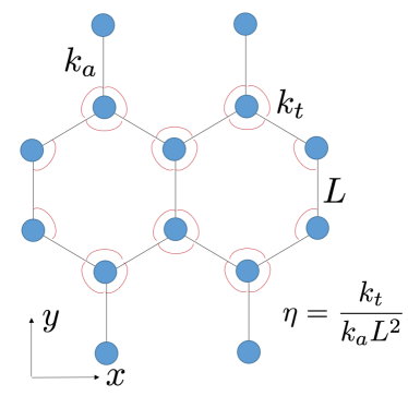
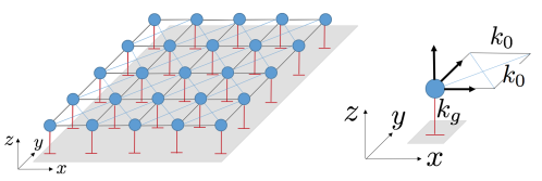
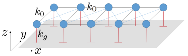
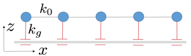
Figure 1: Summary of discrete lattices considered for observation and analysis of instability-induced localization: hexagonal lattice investigated in [15] (a), square lattice with ground springs (left) and detail of unit cell (right) (b), one-dimensional square lattice strip (c), and 1D spring mass chain (d).

2 Background: instability-induced localization in hexagonal lattices

Instabilities in lattices leading to localized deformations or global pattern formation depend on the interplay of several factors, including lattice geometry, material parameters, boundary and loading conditions. The effect of some of these factors is here briefly illustrated as background and motivation for the investigations to follow. We consider the quasi-static behavior of the hexagonal lattice of Fig. 1, which consists of point masses connected by linear longitudinal springs $k_{a}$, and includes angular springs $k_{t}$ that oppose the change in angle between neighboring springs [15, 16]. The lattice is constrained to deform in the $x,y$ plane and undergoes large displacements resulting from the imposed set of displacements. We determine the equilibrium configuration of a finite assembly of $32\times 23$ unit cells by minimizing the potential energy of the lattice at each incremental step of the prescribed displacement using a Newton-Raphson procedure. This procedure is described in detail in [15]. The behavior of the lattice is controlled by a single nondimensional parameter $\eta=k_{t}/k_{a}L^{2}$, which quantifies the relative values of the axial and torsional springs, with $L$ being the distance between the two sub-lattice sites in a unit cell. The case of $\eta=6\times 10^{-3}$ here considered corresponds to a lattice characterized by a non-convex energy and that exhibits complex deformation patterns under uniform loading conditions due to instabilities.

We first illustrate the lattice deformation corresponding to an imposed vertical displacement leading to a total normal strain for the finite lattice of $\delta_{y}=-0.15$. As the imposed displacement is progressively increased, the deformation evolves from being initially affine (linear in $x$ and $y$) to subsequently achieving global patterns as in Fig. 2. These patterns, associated with a long wavelength instability, break the translation invariance of the displacement field in the $x$-direction and their onset coincides with with the loss of rank-one convexity in the potential energy of a single unit cell [15]. Next, we discuss the case of a bi-axial loading corresponding to imposed displacements along both the horizontal and vertical direction, leading to normal strains for the lattice domain respectively equal to $\delta_{x}=-0.2$ and $\delta_{y}=0.2$. The resulting deformed configuration shown in Fig. 2 is characterized by a localized deformation along a “zig-zag” interface. This pattern of localized deformation is attributed to the competition between two factors: localized deformation along the unit vector direction and the imposed affine boundary conditions.

Finally, we illustrate how the localization pattern can vary with boundary conditions. Figure 2 displays the deformation pattern when periodic boundary condition are imposed along with a prescribed horizontal normal strain $\delta_{x}=-0.12$. In contrast to the case in Fig. 2, localization occurs along one of the lattice vector directions, at an angle $2\pi/3$ from the $x$-axis. Indeed the change in localization pattern compared to the previous case is attributed to relaxing the affine displacement constraint on the top and bottom surface nodes. Thus the deformation patterns that result in these nonlinear lattices depend on their geometry, lattice parameters or material properties, loading and boundary conditions. Elucidating the interplay between these factors is a daunting challenge, and is the subject of ongoing investigations. To address some of the questions that the observations presented above pose, we here focus on the effects of lattice parameters under a single, uni-axial loading condition. To this end, we elect to investigate the lattices in Fig. 1-1, which are characterized by a simpler geometry described by orthogonal lattice vectors, but which however have a potentially richer behavior related to the ability of deform both in-plane and out-of-plane. The interaction of these deformations and their relation to the onset of various instabilities will be investigated in lattices of increasing simplicity in an attempt to obtain general insight into the unique mechanism observed herein.

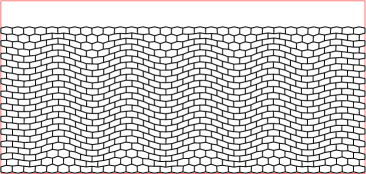
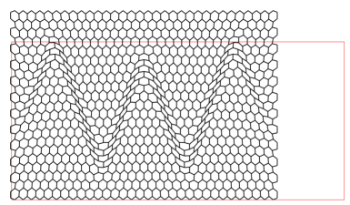
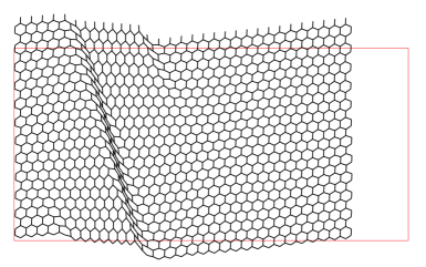
Figure 2: Deformed configurations having different localization patterns for different boundary conditions. (a) Biaxial loading with displacement prescribed on all boundary nodes; (b) compression prescribed on horizontal direction and periodic conditions along vertical boundary nodes; (c) compression prescribed on horizontal direction, free to expand and periodic conditions in vertical direction.

3 Square lattice model

Let us consider a square lattice of $N\times M$ nodes, that is $(N-1)\times(M-1)$ unit cells, which includes point masses at the nodes and three types of springs connecting them. In contrast to the previous hexagonal lattice case where the masses were restricted to move in the $xy$-plane, here each point mass has $3$ translational degrees of freedom and can move in three spatial dimensions. The diagonal springs and the springs connecting nearest neighbors both have stiffness $k_{0}$. There is a ground spring of stiffness $k_{g}$, which resists motion in the out-of-plane $z$ direction. The quasi-static behavior of a lattice of a given dimension is governed by a single nondimensional stiffness parameter, $\gamma=k_{g}/k_{0}$. In all the subsequent calculations in this work, we investigate the behavior of a lattice under uniaxial compression. Both the in-plane displacement components are prescribed at all the boundary nodes corresponding to this uniaxial strain, while the out-of-plane displacement component is free at all the nodes.

3.1 In-plane and out-of-plane instability

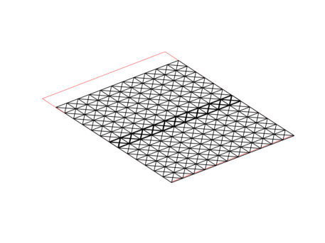
Figure 3: Two kinds of instabilities in square lattices subjected to compression. The deformation is in-plane and globally uniform at high stiffness parameter $\gamma=1.0$ (a) in contrast to the out of plane and localized deformation at low $\gamma=0.1$ (b).

We first investigate the quasi-static behavior of this lattice under uniaxial compression along $x$-direction with the strain denoted by $\delta_{x}$. To this end, we conduct numerical simulations to determine the deformed configuration by increasing the strain incrementally from the undeformed configuration. At each strain level, the equilibrium configuration is obtained by minimizing the potential energy $E$ of the lattice subject to the appropriate boundary conditions. The problem may be expressed as

$$\underset{\mathbf{X}}{\text{minimize}} E(\mathbf{X})=\dfrac{k_{0}}{2}\sum_{m=1}^{M-1}\sum_{n=1}^{N-1}\bigl{[}\left(\|\bm{x}_{m,n}-\bm{x}_{m+1,n}\|-a\right)^{2}+\left(\|\bm{x}_{m,n}-\bm{x}_{m,n+1}\|-a\right)^{2}+$$ (1)

$$\;\;\;\;\;\;\;\left(\|\bm{x}_{m,n}-\bm{x}_{m+1,n+1}\|-\sqrt{2}a\right)^{2}+\left(\|\bm{x}_{m+1,n}-\bm{x}_{m,n+1}\|-\sqrt{2}a\right)^{2}\bigr{]}+$$

$$\;\;\;\;\;\;\;\dfrac{k_{g}}{2}\sum_{m=1}^{M}\sum_{N=1}^{N}z_{p}^{2}$$

subject to $$x_{q}=(1+\delta_{x})X_{q},\;y_{q}=0\;\;\;q=1,\ldots,N_{b},$$

$$z_{q}=0\;\;\;q=1,\ldots N_{c}.$$

Here $N_{b}$ is the total number of boundary nodes, $N_{c}$ is the nodes on the boundary along the $y$-direction, while $(X_{p},Y_{p},Z_{p})$ and $\bm{x}_{p}=(x_{p},y_{p},z_{p})$ denote, respectively, the undeformed and deformed positions of node $p$ and $\mathbf{X}=(\bm{x}_{1,1},\bm{x}_{1,2},\ldots,\bm{x}_{M,N})$. Finally, $a$ is the distance between nearest neighbor masses in the lattice.

Figure 3 illustrates the typical deformation field for two values of stiffness parameter $\gamma$. The two chosen $\gamma$ values are representative of the behavior of lattices with high and low $\gamma$. Figure 3 displays the in-plane deformation field when $\gamma=1.0$. The out-of-plane displacement is zero and globally uniform patterns form after the onset of an instability. The displacement field is affine for small strains $\delta$ near the undeformed configuration. This range of $\delta$ may be determined numerically using a procedure similar to the stability analysis presented later in Sec. 4.2. With increasing strain, this affine solution loses stability leading to the evolution of globally uniform patterns with a wavelength of two unit cells along the loading direction and uniform along the transverse in-plane direction. We remark here that this deformation mode arises as a bifurcation since the affine solution satisfies the equilibrium equations. Figure 3 displays the deformation field for a square lattice with a lower stiffness parameter value $\gamma=0.1$. Here the deformation happens along the out-of-plane direction too and leads to a localization which consists in one layer of the lattice folding over its adjacent layer. We observe that the deformation field is essentially two dimensional with no displacement in the transverse in-plane direction ($y$). Thus we see that the patterns that form after the onset of a bifurcation depend on the material property, stiffness parameter $\gamma$ in this case, and it can range from globally uniform patterns to localized folding behavior.

3.2 Deformation sequence leading to localization

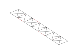
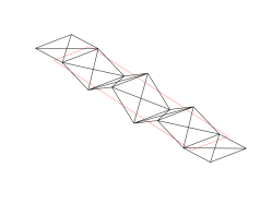
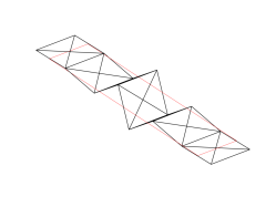
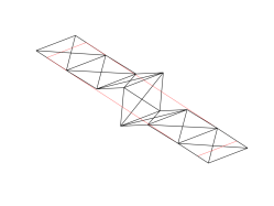
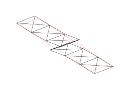
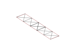
Figure 4: Snapshots of the folding transition process from the fully expanded and undeformed configuration (a) to the folded configuration (f), $\gamma=0.1$. The process involves two distinct bifurcations, with the vertical deformation first increasing globally and then getting localized at the center as the lattice is compressed.

Let us examine the sequence of deformations that result in a localized folding pattern in a lattice with $\gamma=0.1$. Since there is no displacement in the transverse in-plane direction, we consider a single strip of the square lattice with $N\times M=2\times 8$ nodes. Figure 4 illustrates the sequence of deformations as this lattice is subjected to a uniaxial compression. For small strains close to the undeformed configuration, the deformation field is affine and there is no out-of-plane displacement. As the strain increases, this affine solution becomes unstable and the lattice deforms out-of-plane in a zig-zag manner (Fig. 4). The out-of-plane displacement is maximum at the center and decreases away from it. As the strain increases further (Fig. 4), the out-of-plane displacement increases for the center nodes, while it decreases for nodes away from the center. The out-of-plane displacement becomes localized at the two center nodes of the lattice and it decreases rapidly to zero away from these nodes. As the strain increases, the center square folds over (Fig. 4-(f)), thereby resulting in a localized zone. Note that this localized deformation field will have zero energy at a strain level $\delta=-2/(M-1)\approx-0.29$ when all the axial springs are unstretched and the out-of-plane displacement is zero. The existence of multiple zero energy states (undeformed and folded configurations) implies that the potential energy is not quasi-convex. It also points to the existence of negative stiffness regions and the possibility of this lattice to exhibit hysteresis. A negative effective stiffness results in a snap-through type behavior as the lattice transitions from the unfolded to the folded configuration or vice versa. We examine this rich set of behaviors arising due to this localized solution in the next section using a one-dimensional model which turns out to be quite adequate for our purposes.

4 Chain on elastic support

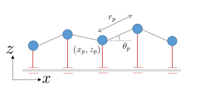
Figure 5: Schematic of a $1D$ lattice model, with point masses at the nodes interacting with nearest neighbor horizontal springs and vertical ground springs. Each mass has two degrees of freedom and can move in the $xz$-plane.

To understand the mechanism of the snap-through behavior during localization, let us further simplify the square lattice and consider an equivalent $1D$ (one-dimensional) model obtained by taking one section of the square lattice deprived of the diagonal springs. Figure 5 displays a schematic of the considered lattice model. There are $N$ nodes along a strip indexed from $1$ to $N$. The potential energy $E$ of the lattice may be written as

$$E(\mathbf{X})=\sum_{i=1}^{N}\dfrac{k_{g}}{2}z_{i}^{2}+\sum_{i=1}^{N-1}\dfrac{k_{0}}{2}\left(\|\bm{x}_{i}-\bm{x}_{i+1}\|-a\right)^{2}.$$ (2)

where $\bm{x}_{i}=(x_{i},z_{i})$ and $\mathbf{X}=(\bm{x}_{1},\bm{x}_{2},\ldots,\bm{x}_{N})$. Here we can assume that the undeformed axial springs have unit length ($a=1$). Minimizing this energy subject to the boundary conditions yields the equilibrium configuration. We illustrate the typical displacement response history as the folding transition happens in this model, see Fig. 6.

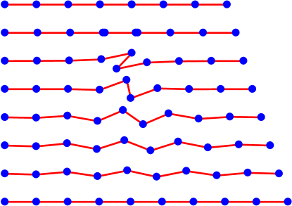
Figure 6: Sequence of deformed configurations as the lattice transitions from the folded to the unfolded configuration.

We first conduct numerical simulations on a lattice of $N=10$ masses by subjecting it to both a compressive strain from the unfolded configuration and a tensile strain from the folded configuration. For both cases, we denote the strain by $\delta$, measuring it from the reference unfolded configuration. The numerical simulations are again conducted using a Newton-Raphson solver. This numerical solver based on incrementally applying strain faces convergence issues in the presence of instabilities and bifurcations. To overcome these limitations, we develop alternative techniques in Sec. 4.3.

4.1 Folding behavior

This $1D$ model also undergoes a folding based localization and we will analyze the deformation process leading to this localization in detail. In all our subsequent calculations, we consider a chain of 10 point masses (nodes) connected by axial springs of stiffness $k_{0}$. Similar to the square lattice, each mass is also connected to the ground by a spring of stiffness $k_{g}$ and the quasi-static behavior is then governed by the non-dimensional stiffness parameter $\gamma=k_{g}/k_{0}$. The chain starts from $x=0$ and the undeformed lattice spans from $x_{1}=0$ to $x_{10}=9$. This is referred to as the unfolded configuration. The first mass is kept fixed while the last mass is subjected to a compressive displacement. The two end masses are also restricted from moving vertically ($z_{1}=z_{10}=0$). As the prescribed compressive displacement increases, the lattice folds at the center and now spans from $x_{1}=0$ to $x_{10}=7$. This is referred to as the folded configuration. Thus we have that $\delta=0$ for the unfolded configuration while $\delta=-2/9$ for the folded one. Figure 6 displays snapshots of the deformed lattice as it deforms from one configuration to the other. We will analyze the quasi-static response of the lattice as it deforms from the folded to the unfolded configuration and vice versa.

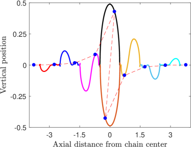
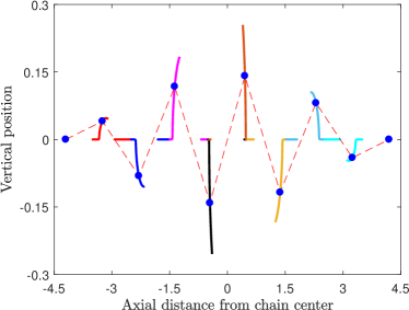
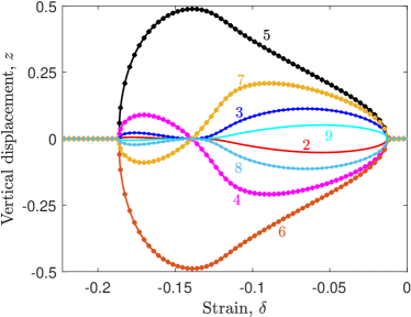
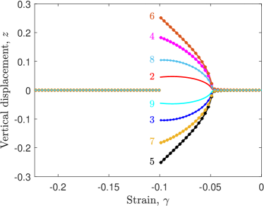
Figure 7: Vertical displacement of the nodes as the lattice is pulled from the folded configuration. Two bifurcation points are observed at low stiffness parameter $\gamma=0.05$ (a, c), while a single bifurcation and a jump in displacement is obtained at high $\gamma=0.2$(b, d).

Figure 7 displays the vertical displacement of the nodes as this lattice is subjected to a tensile strain from the folded configuration. Note that the lattice in the initial configuration spans from $x_{1}=0$ to $x_{10}=7$ in the axial direction. As the lattice is pulled from both ends, it reaches a final unfolded and undeformed configuration ranging from $0$ to $9$. The horizontal and vertical axes show, respectively, the compressive strain $\delta$ measured from the reference unfolded configuration and the vertical displacement of all the nodes in between. Figure 7 displays the displacements for stiffness parameter $\gamma=0.1$. At small displacements from the initial configuration, the axial displacement field is affine in the lattice and the vertical displacement is zero. At around $\delta=-0.187$, there is an instability and the lattice deforms out of plane, thereby initiating the unfolding process. The vertical displacement decreases away from the center nodes and it increases with increasing tensile strain near the bifurcation point. The nodes to the right of the center spring have a positive vertical displacement while the corresponding nodes to the left have an equal and opposite vertical displacement.

As the tensile strain increases, the vertical displacement of the nodes away from the center decrease to zero at around $\delta=-0.139$. Beyond this point, the shape of the displacement field changes as the vertical displacement of adjacent nodes alternate in sign. They first increase and then decrease in magnitude, reaching a zero value at around $\delta=-0.011$. Beyond this point, the displacement field is affine in the axial direction and has no vertical component. This deformation mode corresponds to uniform compression of the lattice from the unfolded and undeformed position, which is attained at $x_{10}=9$. We thus see two distinct mode-shapes arising from the onset of two bifurcation points as the lattice deforms from the folded to the unfolded configuration. We address the mechanism of transformation from one mode-shape to another using a reduced $4$-mass model later in Sec. 4.3.2.

Let us now examine the displacement when a lattice with a higher stiffness parameter value $\gamma=0.2$ is subjected to a similar tensile strain. Figure 7 displays the vertical displacement of the interior nodes ($z_{2}$ to $z_{9}$) as it deforms from the folded to the unfolded configuration. In contrast to the low stiffness parameter case, here the vertical displacement remains zero for larger tensile strains until around $\delta=-0.1$, when the vertical displacement jumps sharply to a non-zero value. The vertical displacement of the adjacent nodes has opposite sign and resembles the second mode-shape discussed above. As the tensile strain increases, the vertical displacement decreases and reaches zero at around $\delta=-0.044$. Beyond this point, the vertical displacement remains zero and the axial displacement is affine with equal compressive strain in each of the axial springs.

4.2 Linear stability analysis

To investigate the local stability of the equilibria computed above, we need to look at the Hessian $\bm{H}$ of the energy $E(\mathbf{X})$, in (2). For a chain having $N$ masses it can be expressed as

$$\bm{H}=\bm{I}_{N}\otimes\begin{pmatrix}0&0\\ 0&\gamma\end{pmatrix}+\sum_{p=1}^{N-1}\bm{K}_{h,p},$$ (3)

where $\bm{I}_{N}$ is the $N\times N$ identity matrix and $\otimes$ denotes the tensor product. Here $\bm{K}_{h,p}$ is the contribution due to the $p$-th axial spring having a deformed length $r_{p}$, with an angle $\theta_{p}$ with respect to the horizontal axis, see Fig. 5. It can be written as

$$\bm{K}_{h}=\mathbf{D}_{p}\otimes(\bm{R}_{p}\bm{K}_{loc,p}\bm{R}_{p}^{T}).$$ (4)

where the $\mathbf{D}_{p}$ is a $N\times N$ matrix what all 0 entries but for the $(p,p+1)$ principal minor,

$$\mathbf{D}_{p}=\bordermatrix{&&&p&p+1&&\cr&0&\cdots&\cdots&\cdots&\cdots&0\cr&\vdots&\ddots&&&\vdots&\vdots\cr p&0&\cdots&1&-1&\cdots&0\cr p+1&0&\cdots&-1&1&\cdots&0\cr&\vdots&\vdots&&\ddots&\vdots\cr&0&\cdots&\cdots&\cdots&\cdots&0}\ ,$$

while $\bm{R}_{p}$ is the rotation of angle $\theta_{p}$ and $\bm{K}_{loc,p}$ is related to the stiffness of the axial spring in the local coordinate system aligned with the spring axis:

$$\bm{R}_{p}=\begin{pmatrix}\cos\theta_{p}&-\sin\theta_{p}\\ \sin\theta_{p}&\cos\theta_{p}\end{pmatrix},\qquad\bm{K}_{loc,p}=\begin{pmatrix}1&0\\ 0&1-\dfrac{1}{r_{p}}\end{pmatrix}\;\;\;.$$ (5)

It is easy to observe that if all the springs are horizontal, that if $\theta_{p}=0$ or $\pi$ for every $p$, then the $x$ and the $z$ part of the Hessian $\bm{H}$ decouple. More precisely, let $\mathbf{P}$ be the permutation matrix that send $\mathbf{X}$ to $\widetilde{\mathbf{X}}=(x_{1},x_{2},\ldots,x_{N},z_{1},z_{2},\ldots,z_{N})=(X,Z)$ then we get

$$\widetilde{\bm{H}}=\mathbf{P}\bm{H}\mathbf{P}^{T}=\begin{pmatrix}\bm{H}_{x}&0\\ 0&\bm{H}_{z}\end{pmatrix}.$$

Moreover one can verify that the $x$ part of the Hessian $\bm{H}_{x}$ is always positive definite. Thus to analyze the stability of an equilibrium with no displacement in the $z$ direction we just need to look at the eigenvalues of $\bm{H}_{z}$.

Let us consider a lattice compressed from its initial unfolded configuration to a strain $\delta$. The affine deformation induced by such a strain is given by $x_{p}=(1+\delta)p$ and $z_{p}=0$ for all $p$. This is clearly an equilibrium configuration. Since the first and last mass are fixed, the stability of this configuration is controlled by the eigenvalues of the $(N-2)\times(N-2)$ matrix

$$\bm{H}_{z}^{u}=\bordermatrix{&2&3&&&N-2\cr 2&\alpha&\zeta&0&\cdots&0\cr 3&\zeta&\alpha&\zeta&\cdots&0\cr\vdots&\ddots&\ddots&\ddots&\vdots\cr N-3&0&\cdots&\zeta&\alpha&\zeta\cr N-2&0&\cdots&0&\zeta&\alpha},$$ (6)

where

$$\alpha=\gamma+\dfrac{2\delta}{1+\delta},\;\;\zeta=-\dfrac{\delta}{1+\delta}.$$ (7)

By looking for eigenvectors $X_{p}$ of the form $X_{p,q}=\sin(\omega_{p}(q-1))$, $q=2,\ldots,N-1$, one immediately gets $\omega_{p}=\pi p/(N-1)$ with associated eigenvalue

$$\lambda_{p}=\gamma+\frac{2\delta}{1+\delta}\left(1-\cos(\omega_{p})\right)$$

and $p=1,\ldots,N-2$. Thus at the critical strain

$$\delta^{*}_{u}=\frac{-\gamma}{\gamma+2\left(1-\cos(\omega_{N-2})\right)}$$

$\lambda_{N-2}$ becomes negative and the affine configuration looses stability. The associated mode shape is given by

$$X_{N-2,q}=\sin\left(\frac{(N-2)(q-1)\pi}{N-1}\right)$$

that shows a maximum value at the center which explains the high deformation, which leads to subsequent folding at the center. The strain value and mode shape predicted by the above stability analysis is in excellent agreement with the numerical solution.

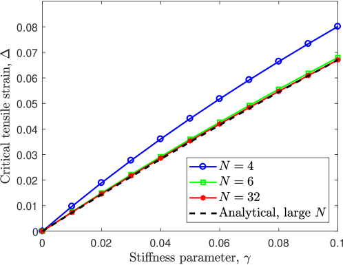
Figure 8: Tensile strain in the axial spring with stiffness parameter $\gamma$ at the onset of unfolding for three different chain lengths. A chain of six masses can essentially capture the onset of bifurcation from the folded configuration of a much large chain with reasonable accuracy.

Let us now consider what happens when a folded lattice is stretched. The folded reference configuration is given by $z_{p}=0$ for all $p$ while $x_{p}=p-1$ if $p\leq N/2$ and $x_{p}=p-3$ if $p>N/2$. Thus the strain of this configuration is $\delta=-2/(N-1)$. If we stretch this configuration and look for an equilibrium still having $z_{p}=0$ for all $p$ we need all springs but the central folded one to have the same strain $\Delta$ while the central one has strain $-\Delta$. We thus get $x_{p}=(p-1)(1+\Delta)$ if $p\leq N/2$ while $x_{p}=(p-2)(1+\Delta)-(1-\Delta)$ if $p>N/2$. The total strain $\delta$ of this configuration is thus $\delta=\Delta-2/(N-1)$. Again we want the critical value of $\Delta$, and thus $\delta$, for which this configuration looses stability.

The Hessian $\bm{H}^{f}_{z}$ in this configuration is similar to (6), that is

$$\bm{H}^{f}_{z}=\begin{pmatrix}\alpha_{2}&\zeta_{2}&0&\cdots&0\\ \zeta_{2}&\alpha_{3}&\zeta_{3}&\cdots&0\\ \vdots&\ddots&\ddots&\ddots&\vdots\\ 0&\cdots&\zeta_{N-3}&\alpha_{N-2}&\zeta_{N-2}\\ 0&\cdots&0&\zeta_{N-2}&\alpha_{N-1}\end{pmatrix},$$ (8)

where

$$\alpha_{p}=\gamma+\frac{2\Delta}{1+\Delta}\qquad\zeta_{p}=-\frac{\Delta}{1+\Delta}$$

for all $p$ but for

$$\alpha_{\frac{N}{2}}=\alpha_{\frac{N}{2}+1}=\gamma+\frac{\Delta}{1+\Delta}-\frac{\Delta}{1-\Delta}\qquad\zeta_{\frac{N}{2}}=\frac{\Delta}{1-\Delta}\ .$$

Let $\mathbf{Q}$ be the reflection matrix such that $(\mathbf{Q}X)_{p}=X_{N-p}$. Clearly $\bm{H}^{f}_{z}$ commutes with $\mathbf{Q}$ so that we know all eigenvectors $X$ of $\bm{H}^{f}_{z}$ must satisfy $\mathbf{Q}X=\pm X$. This means that they are either symmetric or anti-symmetric with respect to the reflection $p\to N-p$. Taking this into consideration, we find that the search for the eigenvalues of $\bm{H}^{f}_{z}$ can be reduced to that of the eigenvalues of the two $(N/2-1)\times(N/2-1)$ matrices given by

$$\bm{H}_{\pm}=\begin{pmatrix}\alpha&\zeta&&&\\ \zeta&\alpha&\zeta&0&\\ &&\ddots&&\\ &0&&\alpha&\zeta\\ &&&\zeta&\beta_{\pm}\end{pmatrix},$$ (9)

where

$$\alpha=\gamma+\dfrac{2\Delta}{1+\Delta},\qquad\zeta=-\dfrac{\Delta}{1+\Delta}$$ (10)

and

$$\beta_{+}=\gamma+\dfrac{\Delta}{1+\Delta}\qquad\beta_{-}=\gamma+\dfrac{\Delta}{1+\Delta}-\dfrac{2\Delta}{1-\Delta}\ .$$

Here $\beta_{+}$ refers to the symmetric eigenvalues while $\beta_{-}$ to the anti-symmetric ones.

As before it is natural to look for eigenvectors $X_{p}$ of the form $X_{p,q}=\sin(\omega_{p}(q-1))$, $q=2,\ldots,N/2-1$. This leads to the condition

$$(\beta_{\pm}-\alpha)\sin(\omega M)=\zeta\sin(\omega(M+1))$$

where $M=N/2-1$.

In the symmetric case this reduces to

$$\sin(\omega M)=\sin(\omega(M+1))$$

so that we get the solutions $\omega_{p}=\pi p/(2M+1)$ with eigenvalue $\lambda_{p}=\alpha+2\gamma\cos(\omega_{p})$. It is easy to see that these eigenvalues are always positive for $\Delta>0$. In the anti-symmetric case we get

$$\sin(\omega(M+1))=\dfrac{3+\Delta}{1-\Delta}\sin(\omega M).$$ (11)

Observe that since

$$\dfrac{3+\Delta}{1-\Delta}>\dfrac{M+1}{M}$$

then (11) admits also exactly one complex solution $\omega_{r}=i\nu^{r}$. The associated eigenvector is thus $X^{r}_{q}=\sinh\nu^{r}(q-1)$ with eigenvalue $\lambda^{r}=\alpha+2\gamma\cosh(\nu^{r})$. A complete basis of eigenvectors is then obtained from the real solution of (11). It is not hard to see that if $\omega$ is real than the associated eigenvalue is positive for $\Delta>0$.

It is not easy to give an exact expression for $\nu^{r}$ for finite $r$. If we take the limit $M\to\infty$ and assume that $\nu^{r}$ has a limit, we obtain, after some algebra,

$$\cosh(\nu^{r})=\frac{1}{2}\left(\frac{3+\Delta}{1-\Delta}+\frac{1-\Delta}{3+\Delta}\right)=\frac{5+2\Delta+\Delta^{2}}{3-2\Delta-\Delta^{2}}$$

so that

$$\lambda^{r}=\frac{(\gamma+4)\Delta^{2}+2(\gamma+2)\Delta-3\gamma}{\Delta^{2}+2\Delta-3}$$

We thus obtain that the critical strain at which the folded configuration loses stability is given by

$$\Delta^{*}=\frac{-(\gamma+2)\pm 2\sqrt{(\gamma+2)^{2}-3}}{\gamma+4}.$$ (12)

To evaluate how close the above asymptotic value of $\Delta^{*}$ is to the real value for finite $N$ we computed $\Delta^{*}$ numerically. Since the eigenvalues of $\bm{H}_{-}$ in (9) are distinct, only one can become zero at the onset of the instability and thus the stability of this configuration can be evaluated by simply examining the sign of the determinant of the matrix $\bm{H}$.

Figure 8 displays the critical tensile strain $\Delta^{*}$ at the onset of the unfolding bifurcation transition for a range of stiffness parameter values. Three distinct chain lengths are considered, with $N=4,6$ and $32$ point masses. In each case, the critical spring length increases almost linearly with the stiffness parameter $\gamma$. Furthermore, this critical value in a finite chain converges rapidly to the corresponding value in an infinite chain. Indeed, the critical strain in a chain with $6$ masses is quite close to that in the $32$ mass chain.

4.3 Unfolded to folded transitions

Having clarified the folding transition and identified the onset of bifurcation points using a stability analysis, let us now turn attention to analyzing the transition path between the two zero energy configurations. We use two numerical techniques for this purpose. We first develop and use a shooting method based procedure to investigate this folding transition in detail in Sec. 4.3.1. We use this method to illustrate the stability regions as $\gamma$ increases and the associated hysteretic behavior. For a moderate number of masses, 10 in our present study, we found this approach hereafter outlined useful in understanding the bifurcation structure. We are aware that this approach may have limitations for large number of masses. We then use a classical arc length solver based continuation scheme in Sec. 4.3.2 on a further simplified four mass chain which confirms the folding transition.

4.3.1 Shooting method for ten mass chain

Here we cast the governing equations for the equilibria into the evolution of a dynamical system. Note that the governing equation of an interior node $p$ depends only on its nodal location and the location of its nearest neighbor nodes ($p-1$ and $p+1$). The governing equations may be used to solve for the nodal locations of $p+1$ node if the other two nodal locations are provided. Accordingly, we may write a relation of the form

$$f(\bm{x}_{p+1})=f(\bm{x}_{p},\bm{x}_{p-1})$$ (13)

where $\bm{x}_{p}=(x_{p},z_{p})$. To determine explicit expressions for $\bm{x}_{p+1}$ above, as before we let $x_{p+1}-x_{p}=r_{p}\cos\theta_{p}$ and $z_{p+1}-z_{p}=r_{p}\sin\theta_{p}$. Figure 5 displays a schematic of a part of the chain with the relevant variables.

With this setup, the equilibrium equations for the mass $p$, obtained by resolving the forces due to the springs in the horizontal and vertical directions, may be written as

$$(r_{p}-1)\cos\theta_{p} =(r_{p-1}-1)\cos\theta_{p-1},$$ (14a)

$$(r_{p}-1)\sin\theta_{p} =(r_{p-1}-1)\sin\theta_{p-1}+\gamma z_{p}$$ (14b)

These equations can be unambiguously solved to obtain $r_{p}$ and $\theta_{p}$ as a function of $\bm{x}_{p-1}$ and $\bm{x}_{p}$. An explicit formula for $\bm{x}_{p+1}$ is then easily obtained using

$$x_{p+1}=x_{p}+r_{p}\cos\theta_{p},\;\;z_{p+1}=z_{p}+r_{p}\sin\theta_{p}.$$ (15)

As discussed in Sec. 4.2, the onset of instability for both the folded and unfolded configurations happens along an anti-symmetric mode shape with respect to the reflection $\mathbf{Q}$, see discussion after (8). We thus expect that the deformation process from the unfolded to the folded configuration will pass only through anti-symmetric configurations, that is configurations for which $x_{10}-x_{10-p}=x_{p}$ and $z_{10-p}=-z_{p}$. This is well verified in Fig. 7.

To find an equilibrium configuration for the chain, we first fix $\bm{x}_{5}$ and as a consequence $\bm{x}_{6}$. Observe that, due to the symmetry of the configuration, this is equivalent to fixing $\theta_{5}$ and $r_{5}$ that from now on we will call $\theta$ and $r$. Once $\bm{x}_{5}$ and $\bm{x}_{6}$ are fixed, we can use (13) to compute $\bm{x}_{7}$ up to $\bm{x}_{10}$ and as a consequence we get a full configuration for the chain.

At this point there is no need for $z_{10}$ to be 0. For a range of value of $r$ we search for the value of $\theta$ for which $z_{10}=0$. Finally we relate back $x_{10}$ to the strain $\delta$. We call this procedure the shooting method to find numerically an equilibrium configuration. Observe that high iterations of $f$ in (13) potentially present stability issues. This is the reason why we decided to compute only anti-symmetric configurations starting from the center of the chain. This is also the reason why the application of this methods to longer chains may require a more refined analysis of the dynamical system generated by $f$.

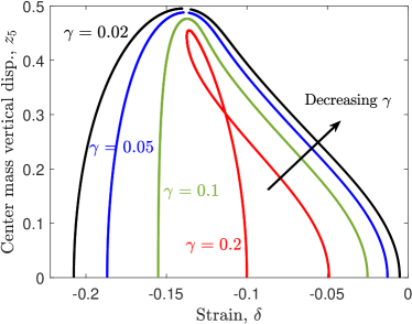
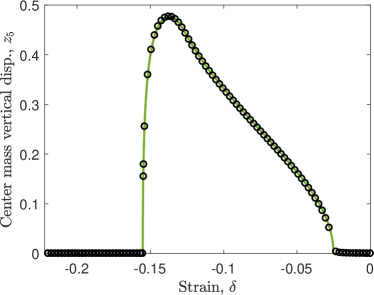
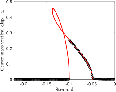
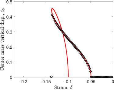
Figure 9: (a) Vertical displacement of the center mass with the axial position of the last mass during the folding process for different stiffness parameter $\gamma$ values. The Newton-Raphosn method solution (black circles) match the shooting method solution (curves) in both loading and unloading for $\gamma=0.1$ (a), while the displacement jumps after the onset of instability in both loading (c) and unloading (d) for $\gamma=0.2$.

To gain further insight into the difference between the high and low stiffness parameter response (Fig. 7) and to understand the displacement jump in Fig. 7, let us examine the solution as the center spring folds. Figure 9 displays the vertical displacement of the center mass $z_{5}$ with compressive strain $\delta$ for $4$ distinct stiffness parameter values. These curves are obtained from the shooting method solution described above. For low $\gamma$, there is a single solution for each strain value in the range $\delta\in[-2/9,0]$. However, as the stiffness parameter $\gamma$ increases, there are three possible solutions in a range of $\delta$ values. This multiplicity of solutions is evident as the curve bends backward yielding two stable and one unstable solution for each $\delta$ value. By comparison, in Fig. 9 we show with black circles the stable solution computed with the previously described Newton-Raphson approach, as the lattice is stretched from the folded to the unfolded configuration. Obviously, there is in excellent agreement with the shooting method solution (solid curve) over the entire range of the folding to unfolding transition. Furthermore, the Newton-Raphson method solution of lattice compression from the unfolded to the folded configuration also matches with this solution.

Let us now examine the response of a lattice having a higher stiffness parameter ($\gamma=0.2$). Figure 9 displays the Newton-Raphson method solution (black circles) as this lattice is stretched from the folded to the unfolded configuration. As we discussed earlier, the solution is unstable for high $\theta$ values and our Newton-Raphson method solution jumps to a stable branch, which corresponds to a lower $\theta$ value. As the displacement increases, the solution follows this branch until $\theta=0$ at around $\delta=-0.049$ after which the vertical displacement of all the nodes is zero. Finally, let us observe the behavior of this lattice as it is compressed to deform from the unfolded to the folded configuration. Figure 9 displays the Newton-Raphson method solution for this case. The Newton-Raphson method solution matches with the shooting method solution until the onset of instability, when the tangent to the red curve in the figure becomes vertical. Beyond this point, our Newton-Raphson solver fails to converge to a stable equilibrium solution. The black circle at around $\delta=-0.138$ indicates the stable solution which a physical system is likely to reach as the prescribed compressive strain increases, which corresponds to a folded configuration and then follows this horizontal branch (coinciding with the previous unfolding case). Thus we observe how the solution can be path dependent for high stiffness parameter $\gamma$ values when there are multiple stable solutions.

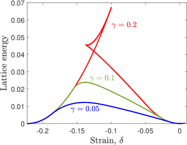
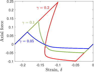
Figure 10: (a) Lattice energy and (b) force acting on the ends of the lattice as it deforms for different stiffness parameter values. As the stiffness increases, the force is not unique in a range of displacements and allows for hysteresis during the folding process.

Having provided evidence for the existence of multiple stable solutions, let us see how the lattice energy and force vary as the lattice deforms from one equilibrium configuration to another. Figure 10 displays the lattice energy in the vertical axis as it deforms from the folded to the unfolded configuration. The strain $\delta$ on the horizontal axis ranges from $-2/9\simeq-0.22$ to $0$. Three curves corresponding to distinct values of stiffness parameter $\gamma$ are shown. In each case, the lattice energy is zero at both the folded and unfolded configurations, resulting in a double well potential in this range of deformations. At low $\gamma$ values, there is a single energy value for each strain $\delta$, while at high $\gamma$, there are multiple energy values consistent with the observations above. For $\gamma=0.2$, we observe that the energy curve has three segments and folds back at around $\delta=-0.138$ and $-0.1$. The middle segment joining the two end segments corresponds to the unstable branch.

Let us now illustrate how the corresponding horizontal force $F$ acting on the chain varies during the folding process. It is defined as the derivative of the potential energy with respect to the chain length, given by

$$F=\dfrac{1}{N-1}\dfrac{\partial E}{\partial\delta}$$

and it is computed by taking the numerical derivative of the energy illustrated in Fig. 10. Figure 10 illustrates the force for the same three stiffness parameter values $\gamma$. In all cases, the force is zero in the folded and unfolded configurations at $\delta=-2/9$ and $\delta=0$. For low stiffness parameter values ($\gamma=0.05$ and $\gamma=0.1$ in the figure), there is again a unique force for each strain value $\delta$. The force displacement response has three segments: two linear and one segment in the middle joining them. The linear segments correspond to affine horizontal deformation about the folded and unfolded configurations. The middle segment corresponds to the rotation of the center spring as $\theta$ varies from $0$ to $\pi$ and the effective stiffness of the chain is negative in this regime as the force decreases with increasing prescribed displacement or tensile strain. Furthermore, there are multiple values of force in a range of strains $\delta$ for the $\gamma=0.2$ high stiffness parameter case. In this range of displacements, there are two stable solutions and one unstable branch. The force-displacement response illustrates the potential for achieving hysteresis in our lattice in two ways. By prescribing displacement and alternating between the folded and unfolded configurations in a lattice with high stiffness parameter $\gamma$, the lattice follows a different path around the unstable branch. For example, in Fig. 10, the force jumps down from $0.24$ to $-0.088$ while unfolding and it jumps up from $-0.042$ to $0.17$ while folding.

Remark 1.

We finally briefly remark on the alternative possibility of inducing hysteresis by exploiting the negative stiffness zone. Instead of prescribing displacement, if we prescribe a horizontal force at the ends of the chain, then the lattice solution will jump at the end of the first segment for all the three stiffness values, for example at a force level $F=-0.026$ from $\delta=-0.013$ while folding and at a force level $F=0.0710$ from $\delta=-0.187$ while unfolding. Thus our results illustrate the potential for hysteresis and localization guided programmable smart materials in lattice based media.

4.3.2 Arc length method for four mass chain

Here we consider the simplest case of $N=4$, that is a chain of $4$ point masses anchored at its extremes. As in previous sections, the unfolded and folded configurations of the four masses are

$$(0,0),\,\ (1,0),\,\ (2,0),\,\ (3,0)\ \quad\text{and}\quad(0,0),\,\ (1,0),\,\ (0,0),\,\ (1,0)\ .$$

We can (and will) parametrize the $x$-coordinate of the last mass as $3l$, with $1/3\leq l\leq 1$, ranging through the folded and unfolded states. Alternatively, we can use the strain, which is related to $l$ by the linear relation

$$\delta=l-1\in[-2/3,\ 0].$$

Calling $\bm{x}_{i}=(x_{i},z_{i})$ the position of the $i$-th point mass, the energy of the system, expressed in nondimensional form by normalizing it by a reference energy $k_{0}a^{2}/2$ is

$$E=\frac{\gamma}{2}\sum_{i=1}^{4}z_{i}^{2}\,+\,\frac{1}{2}\sum_{i=1}^{3}(\|\bm{x}_{i+1}-\bm{x}_{i}\|-1)^{2}$$ (16)

where the first sum is the potential energy of the vertical restoring force and the last sum is the potential energy of the springs. In this last sum $\bm{x}_{1}$ and $\bm{x}_{4}$ represent the fixed extreme of the chain, namely $\bm{x}_{1}=(0,0)$, $\bm{x}_{4}=(3l,0)$.

Now, with $N=4$, we assume that the equilibrium position satisfies $x_{3}=3l-x_{2}$ and $z_{3}=-z_{2}$. Let us call $r$ the length of the segment from the middle point to the location of the second point mass $\bm{x}_{2}$, and call $\theta$ the angle formed between the middle point and the horizontal. This way, the 4 point masses get located at the points:

$$\bm{x}_{1}=(0,0),\,\ \bm{x}_{2}=(3l/2-r\cos\theta,\ r\sin\theta),\,\ \bm{x}_{3}=(3l/2+r\cos\theta,\ -r\sin\theta),\,\ \bm{x}_{4}=(3l,0)\ .$$

Clearly we have only the variables $r$ and $\theta$ to consider and the potential to minimize becomes

$$E(r,\theta)=\gamma r^{2}\sin^{2}\theta+\left(\sqrt{r^{2}-3lr\cos\theta+\frac{9l^{2}}{4}}-1\right)^{2}+\frac{1}{2}\left(2r-1\right)^{2}$$

so that by taking derivatives we get the necessary conditions

$$\begin{split}E_{r}\equiv 2\gamma r\sin^{2}\theta+\left(2r-3l\cos\theta\right)\left(1-\left(r^{2}-3lr\cos\theta+\frac{9l^{2}}{4}\right)^{-\frac{1}{2}}\right)+2(2r-1)=&0\\ E_{\theta}\equiv 2\gamma r^{2}\sin\theta\cos\theta+3lr\sin\theta\left(1-\left(r^{2}-3lr\cos\theta+\frac{9l^{2}}{4}\right)^{-\frac{1}{2}}\right)=&0\ .\end{split}$$ (17)

Now, observe that there are two solutions valid for all $\gamma$:

Unfolded

$r=l/2$ and $\theta=0$;

Folded

$r=\frac{2}{3}-\frac{l}{2}$ and $\theta=\pi$.

Unlike our previous numerical experiments, here we implement a classic pseudo-arc-length continuation algorithm starting with the trivial solution branch $(l/2,0)$ for $l$ ranging from $l=1$ to $l=1/3$, and monitoring branch points originating from this branch. Further following this bifurcating branch, we will eventually connect the branch $(l/2,0)$ to the other solution branch $(\frac{2}{3}-\frac{l}{2},\pi)$. Stability monitoring is done by looking at the Hessian eigenvalues. In the graphs below, we show what happens for several different values of $\gamma$. The most insightful visualizations are obtained displaying the values of $\cos(\theta)$, with the two trivial branches corresponding to the values $1$ and $-1$; when not confusing, we also display the height value, as in the figures of the previous sections. We will show in bold-face the stable portions of the equilibria branches. In spite of different values of $\gamma$, the picture we obtain in this simple case of $N=4$ is quite similar to what we observed in the previous sections for $N=10$.

For $\gamma$ small ($\gamma=0.1$ in Figure 11-(b)), we have a stable connection of equilibria configurations between the two trivial branches of equilibria. That is, for each value of the strain in $[-2/3,0]$, there is always only one stable stationary solution.

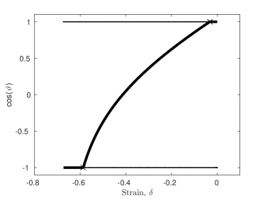
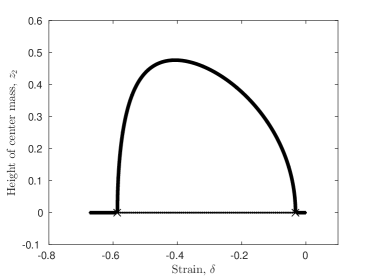
Figure 11: $\gamma=0.1$. Stable equilibria connection between unfolded and folded configurations.

As $\gamma$ grows, the stable connection between the two trivial branches develop a fold and there are two stable equilibrium solutions for a range of values of the strain: one of the trivial branches and (portion of) the connecting branch; see the case of $\gamma=1.05$ in Figure 12-(b).

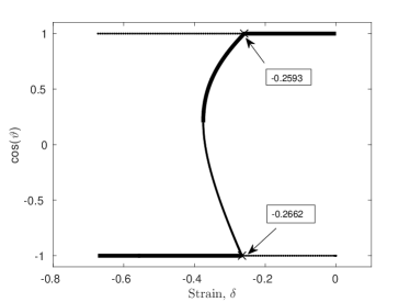
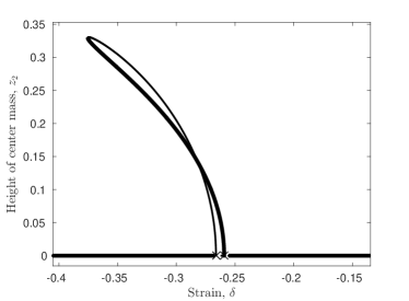
Figure 12: Partially stable equilibria connection between unfolded and folded configurations. Hysteretic behavior.

At the same time, as we increase $\gamma$ further, there is a range of values of the strain where both trivial branches are stable, as well as part of the connecting branch of equilibria; see $\gamma=2$ in Figure 13. Eventually, for $\gamma$ sufficiently large ($\gamma=7$ in Figure 13), the connecting branch is made up entirely of unstable equilibria and the branch points on the trivial branches occur outside the range of values of the unfolded/folded configurations.

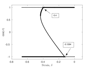
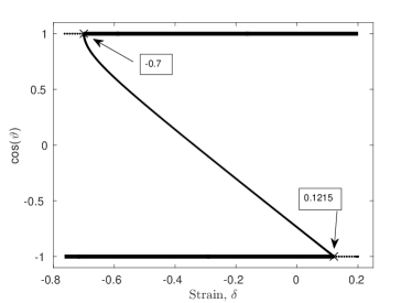
Figure 13: (a) $\gamma=2$. Both folded and unfolded branches are stable for a range of strain values. (b) $\gamma=7$. As $\gamma$ becomes large, the branch of equilibria connecting folded and unfolded states is fully unstable; the states themselves are stable for all strain values.

Remark 2.

As an alternative to the continuation technique we used, we also double checked our results by a more algebraic technique, obtaining the same results. Dividing the second equation in (17) by $r\sin\theta$, and with some algebra, (17) rewrite as

$$\begin{split}(2\gamma r\cos\theta+3l)^{2}\left(r^{2}-3lr\cos\theta+\frac{9l^{2}}{4}\right)=&9l^{2}\\ (2r-3l\cos\theta)\gamma r\cos\theta-3l(\gamma r\sin^{2}\theta+2r-1)=&0\ .\end{split}$$ (18)

From (18), the second equation becomes

$$2\gamma r^{2}\cos\theta-3l((\gamma+2)r-1)=0$$

that is

$$\cos\theta=\frac{3l((\gamma+2)r-1)}{2\gamma r^{2}}$$ (19)

that replaced in the first of (18) gives

$$\left(3l((\gamma+2)r-1)+3lr\right)^{2}\left(8\gamma r^{3}-36l^{2}((\gamma+2)r-1)+18\gamma l^{2}r\right)-72\gamma l^{2}r^{3}=0$$

or

$$18l^{2}\,-\,9l^{2}(5\gamma+16)r\,+\,18l^{2}(\gamma+3)(2\gamma+7)r^{2}\,-\,9l^{2}(\gamma+3)^{2}(\gamma+4)r^{3}\,-\,8\gamma(\gamma+3)r^{4}\,+\,4\gamma(\gamma+3)^{2}r^{5}=0\ .$$

From the roots of this quintic, which we do by finding them as eigenvalues of the associated companion matrix (and keeping only the real ones for which the relative $\cos\theta$ given by (19) is in $[-1,1]$), we obtain the possible equilibrium solutions.

5 Conclusions

To understand, predict and control localization patterns in lattices, we considered a square lattice on an elastic substrate. We exemplified how the type of instability changes from in-plane to out of plane with increasing stiffness parameter. The latter instability evolves to a localized deformation with increasing strain and it is investigated in detail using a one-dimensional lattice. Using a shooting method based approach, we identified the stable branches of deformation as the lattice deforms from one stable configuration to another with a localized deformation. For lattices with low stiffness parameter, there is only one stable solution as the localized pattern forms, while if this spring stiffness exceeds a critical value, there are two stable solutions in a range of displacements. The lattice energy and force response demonstrate the potential for inducing hysteresis due to the existence of the two stable solutions. Finally, we considered the simplest model possible, $4$ point masses with the two endpoints fixed. In this case, we used a classical continuation technique and were able to confirm the transition from unfolded to folded quasi-static equilibrium configurations.

In summary, we have illustrated that, in contrast to many other existing works where localization is unpredictable and sensitive to the presence of defects, localized deformation can be predicted precisely based on geometry and symmetry considerations. Our analysis framework may open avenues for controlled design of interfaces for waveguiding and programmable smart materials applications.

References

- [1] MH Yoo. Slip, twinning, and fracture in hexagonal close-packed metals. Metallurgical Transactions A, 12(3):409–418, 1981.
- [2] N Murisic, V Hakim, IG Kevrekidis, SY Shvartsman, and B Audoly. From discrete to continuum models of three-dimensional deformations in epithelial sheets. Biophysical journal, 109(1):154–163, 2015.
- [3] JG Ramsay. Development of chevron folds. Geological Society of America Bulletin, 85(11):1741–1754, 1974.
- [4] DM Kochmann and K Bertoldi. Exploiting microstructural instabilities in solids and structures: From metamaterials to structural transitions. Applied Mechanics Reviews, 69(5):050801, 2017.
- [5] K Bhattacharya. Microstructure of martensite: why it forms and how it gives rise to the shape-memory effect, volume 2. Oxford University Press, 2003.
- [6] Fan Xu, Michel Potier-Ferry, Salim Belouettar, and Heng Hu. Multiple bifurcations in wrinkling analysis of thin films on compliant substrates. International Journal of Non-Linear Mechanics, 76:203–222, 2015.
- [7] Luka Pocivavsek, Robert Dellsy, Andrew Kern, Sebastián Johnson, Binhua Lin, Ka Yee C Lee, and Enrique Cerda. Stress and fold localization in thin elastic membranes. Science, 320(5878):912–916, 2008.
- [8] G Geymonat, S Müller, and N Triantafyllidis. Homogenization of nonlinearly elastic materials, microscopic bifurcation and macroscopic loss of rank-one convexity. Archive for rational mechanics and analysis, 122(3):231–290, 1993.
- [9] CL Kane and TC Lubensky. Topological boundary modes in isostatic lattices. Nature Physics, 10(1):39–45, 2014.
- [10] MS Anderson and FW Williams. Vibration and buckling of general periodic lattice structures. 1984.
- [11] Jayson Paulose, Anne S Meeussen, and Vincenzo Vitelli. Selective buckling via states of self-stress in topological metamaterials. Proceedings of the National Academy of Sciences, 112(25):7639–7644, 2015.
- [12] N Triantafyllidis and MW Schraad. Onset of failure in aluminum honeycombs under general in-plane loading. Journal of the Mechanics and Physics of Solids, 46(6):1089–1124, 1998.
- [13] JW Hutchinson and X Chen. Herringbone buckling patterns of compressed thin films on compliant substrates. J. Appl. Mech, 71:597–603, 2004.
- [14] K Bertoldi and MC Boyce. Mechanically triggered transformations of phononic band gaps in periodic elastomeric structures. Physical Review B, 77(5):052105, 2008.
- [15] RK Pal, M Ruzzene, and JJ Rimoli. A continuum model for nonlinear lattices under large deformations. International Journal of Solids and Structures, 96:300–319, 2016.
- [16] RK Pal, JJ Rimoli, and M Ruzzene. Effect of large deformation pre-loads on the wave properties of hexagonal lattices. Smart Materials and Structures, 25(5):054010, 2016.
- [17] A Lee, FL Jiménez, J Marthelot, JW Hutchinson, and PM Reis. The geometric role of precisely engineered imperfections on the critical buckling load of spherical elastic shells. Journal of Applied Mechanics, 83(11):111005, 2016.
- [18] C Combescure, P Henry, and RS Elliott. Post-bifurcation and stability of a finitely strained hexagonal honeycomb subjected to equi-biaxial in-plane loading. International Journal of Solids and Structures, 88:296–318, 2016.
- [19] JW Rudnicki and JR Rice. Conditions for the localization of deformation in pressure-sensitive dilatant materials. Journal of the Mechanics and Physics of Solids, 23(6):371–394, 1975.
- [20] LJ Gibson and MF Ashby. Cellular solids: structure and properties. Cambridge university press, 1999.
- [21] SD Papka and S Kyriakides. In-plane compressive response and crushing of honeycomb. Journal of the Mechanics and Physics of Solids, 42(10):1499–1532, 1994.
- [22] SD Papka and S Kyriakides. Experiments and full-scale numerical simulations of in-plane crushing of a honeycomb. Acta materialia, 46(8):2765–2776, 1998.
- [23] SD Papka and S Kyriakides. Biaxial crushing of honeycombs:—part 1: Experiments. International Journal of Solids and Structures, 36(29):4367–4396, 1999.
- [24] MPS d’Avila, N Triantafyllidis, and G Wen. Localization of deformation and loss of macroscopic ellipticity in microstructured solids. Journal of the Mechanics and Physics of Solids, 97:275–298, 2016.