Learning to Emulate an Expert Projective Cone Scheduler

Abstract

Projective cone scheduling defines a large class of rate-stabilizing policies for queueing models relevant to several applications. While there exists considerable theory on the properties of projective cone schedulers, there is little practical guidance on choosing the parameters that define them. In this paper, we propose an algorithm for designing an automated projective cone scheduling system based on observations of an expert projective cone scheduler. We show that the estimated scheduling policy is able to emulate the expert in the sense that the average loss realized by the learned policy will converge to zero. Specifically, for a system with $n$ queues observed over a time horizon $T$, the average loss for the algorithm is $O\left(\ln(T)\sqrt{\ln(n)/T}\right)$. This upper bound holds regardless of the statistical characteristics of the system. The algorithm uses the multiplicative weights update method and can be applied online so that additional observations of the expert scheduler can be used to improve an existing estimate of the policy. This provides a data-driven method for designing a scheduling policy based on observations of a human expert. We demonstrate the efficacy of the algorithm with a simple numerical example and discuss several extensions.

1 Introduction

In a variety of application areas, processing systems are dynamically scheduled to maintain stability and to meet various other objectives. Indeed, the basic problem in scheduling theory has been to find and study policies that accomplish this task under different modeling assumptions. In practice however, while human experts may be able to manage real-world processing systems, it is typically non-trivial to precisely quantify the costs and objectives that govern expert schedulers. For example, in operating room scheduling, ad hoc metrics have been applied in an attempt to model the cost of delays, e.g. [1], but these metrics are largely subjective. The Delphi Method is commonly used in management science to quantitatively model expert opinions but such methods have no algorithmic guarantees and are not always reliable [2].

In this paper, we present an online algorithm that allows us to emulate an expert scheduler based on observations of the backlog of the queues in the system and observations of the expert’s scheduling decisions. We use the term “emulate” to mean that while the parametric form of the learned policy may not converge to the parametric form of the expert policy in all cases, it will always yield scheduling decisions that on average converge to the expert’s decisions. This offers a data-driven way for designing autonomous scheduling systems. We specifically consider a projective cone scheduling (PCS) model which has applications in manufacturing, call/service centers, and in communication networks [3, 4].

The algorithm in this paper uses the multiplicative weight update (MWU) method [5]. The MWU method has been used in several areas including solving zero-sum games [6], solving linear programs [7], and inverse optimization [8]. Because the PCS policy can be written as a maximization, our techniques are most similar to those used in [8]. In [8], the authors apply an MWU algorithm over a fixed horizon to learn the objective of an expert who is solving a sequence of linear programs. Our results differ from [8] in several ways. One is that because of the queueing dynamics that we consider, our expert’s objective will vary over time whereas in [8] the objective is constant. A related issue is that in [8], when the expert has a decision variable of dimension $n$, the dimension of the parameter being learned is also $n$. In our case, when the expert has a decision variable of dimension $n$ (i.e. there are $n$ queues in the system), we need to estimate $\Theta(n^{2})$ parameters. We also note that in this paper we provide an algorithm that can be applied even when the horizon is not known a priori.

The goal of inferring parts of an optimization model from data is a well-studied problem in many other applications. For example, genetic algorithm heuristics have been applied to estimate the objective and constraints of a linear program in a data envelopment analysis context [9]. The goal of imputing the objective function of a convex optimization problem has also been considered in the optimization community, e.g. [10, 11]. These papers rely heavily on the convexity of the objective and the feasible set. This approach does not apply in a PCS context because the set of feasible scheduling actions is discrete and hence non-convex.

This paper is also related to inverse reinforcement learning. Inverse reinforcement learning is the problem of estimating the rewards of a Markov decision process (MDP) given observations of how the MDP evolves under an optimal policy [12]. Inverse reinforcement learning can be used to emulate expert decision makers (referred to as “apprenticeship learning” in the machine learning community) as long as the underlying dynamics are Markovian [13]. In the PCS model, no such assumption is made and so our results naturally do not require Markovian dynamics.

The remainder of this paper is organized as follows. Section 2 specifies the PCS model that we consider. Section 3 presents our algorithms and the relevant guarantees. Because we take a MWU approach to the problem, our guarantees are bounds on the average loss. However, we also provide a concentration bound which gives guarantees on the tail of the loss distribution. We provide a simple numerical demonstration of our algorithms in Section 4. In Section 5 we discuss some extensions of our results and we conclude in Section 6.

2 Projective Cone Scheduling Dynamics

In this section we summarize the PCS model presented in [4] and comment on the connection to the model presented in [3]. The PCS model has $n$ queues each with infinite waiting room following an arbitrary queueing discipline. Time is discretized into slots $t\in\mathbb{Z}_{+}$. The backlog in queue $i$ at the beginning of time slot $t$ is $x_{t}(i)$. The backlog across all queues can be written as a vector $x_{t}\in\mathbb{Z}_{+}^{n}$. The number of customers that arrive at queue $i$ at the end of time slot $t$ is $a_{t}(i)$. The arrivals across all queues can be written as a vector $a_{t}\in\mathbb{Z}_{+}^{n}$. Scheduling configurations are chosen from a finite set $\mathcal{S}\subsetneq\mathbb{Z}_{+}^{n}$. If configuration $s_{t}\in\mathcal{S}$ is chosen in time slot $t$ then for each queue $i$, $\min\left\{s_{t}(i),x_{t}(i)\right\}$ customers are served at the beginning of the time slot. We take the departure vector as $d_{t}=\min\left\{s_{t},x_{t}\right\}\in\mathbb{Z}_{+}^{n}$ where the minimum is taken component-wise. This gives us the following dynamics

$$x_{t+1}=x_{t}-d_{t}+a_{t}$$ (1)

where $x_{0}\in\mathbb{Z}_{+}^{n}$ is arbitrary. Note that the arrival vector is allowed to depend on previous scheduling configurations, previous arrivals, and previous backlogs in an arbitrary way.

The scheduling configurations are dynamically chosen by solving the maximization

$$\max_{s\in\mathcal{S}}\left\langle s,Bx_{t}\right\rangle=\max_{s\in\mathcal{S}}\sum_{i,j}s(i)B(i,j)x_{t}(j)$$ (2)

where $B\in\mathbb{R}^{n\times n}$ is symmetric and positive-definite with non-positive off-diagonal elements. We assume that $\mathcal{S}$ is endowed with some arbitrary ordering used for breaking ties. This PCS policy defines a broad class of scheduling policies and in particular we note that by taking $B$ as the identity matrix, we return to the typical maximum weight matching scheduling algorithm.

Although $B$ is a matrix, because $B$ is symmetric, there are only $p=n(n+1)/2$ rather than $n^{2}$ free parameters that need to be learned. Consequently, we will represent the projective cone scheduler with an upper-triangular array rather than a matrix. In particular, take $b(i,i)\propto B(i,i)$ for $i\in[n]$ and $b(i,j)\propto-B(i,j)$ for $(i,j)\in\left\{(i,j)\in[n]\times[n]:i<j\right\}$. We can also assume without loss of generality that $\sum_{i,j}b(i,j)=1$. Then we can write the projective cone scheduling decision as follows:

$$s_{t} =\arg\max_{s\in\mathcal{S}}\left\langle s,Bx_{t}\right\rangle$$

$$=\arg\max_{s\in\mathcal{S}}\sum_{i=1}^{n}\sum_{j=1}^{n}B(i,j)s(i)x_{t}(j)$$

$$=\arg\max_{s\in\mathcal{S}}\Big{\{}\sum_{i}B(i,i)s(i)x_{t}(i)$$

$$\hskip 49.79231pt+\sum_{i<j}B(i,j)(s(i)x_{t}(j)+s(j)x_{t}(i))\Big{\}}$$

$$=\arg\max_{s\in\mathcal{S}}\Big{\{}\sum_{i}b(i,i)s(i)x_{t}(i)$$

$$\hskip 49.79231pt-\sum_{i<j}b(i,j)(s(i)x_{t}(j)+s(j)x_{t}(i))\Big{\}}$$

$$\triangleq\mu(x_{t};b)$$ (3)

For convenience, let us define

$$\sigma(i,j)=\left\{\begin{array}[]{rc}1&,\,i=j\\ -1&,\,i\neq j\end{array}\right.$$ (4)

so that we we can write $\mu$ more compactly as follows:

$$\mu(x_{t};b) =\arg\max_{s\in\mathcal{S}}\sum_{i\leq j}\sigma(i,j)b(i,j)(s(i)x_{t}(j)+s(j)x_{t}(i))$$ (5)

Note that if we define $y_{t}$, a normalized version of $x_{t}$, as follows,

$$y_{t}=\left\{\begin{array}[]{cl}x_{t}&,\,\left\|x_{t}\right\|_{1}=0\\ x_{t}/\left\|x_{t}\right\|_{1}&,\,\text{otherwise}\end{array}\right.$$ (6)

then we have that $s_{t}=\mu(x_{t};b)=\mu(y_{t};b)$.

Modeling each customer as having a uniform deterministic service time is motivated largely by applications in computer systems and in particular, packet switch scheduling. However, PCS models with non-deterministic service times have also been considered in the literature [3]. However, the results in [3] only apply to the case where $B$ is diagonal. We have opted to present our algorithms in the context of the non-diagonal case because we feel that having $\Theta(n^{2})$ parameters is more interesting than having only $\Theta(n)$ parameters. Our algorithms can still be applied in the case of stochastic service times; this is discussed along with other extensions in Section 5.

Finally, we note that previous literature on PCS [3, 4] has required a variety of additional assumptions. For example, in [4] it is assumed that the arrival process is mean ergodic. We do not require such an assumption and moreover, while the results in [3] and [4] are primarily stability guarantees, we make no assumptions on the stability of the system.

3 The Learning Algorithm

In this section we present our algorithm. We first present a finite horizon algorithm and then leverage this to present an infinite horizon algorithm. For both algorithms, we show that the average error is $O(\ln(T)\sqrt{\ln(p)/T})$. We also provide a bound on the fraction of observations for which the error exceeds our average case bound.

These algorithms are applied causally in an online fashion. Although we do not focus on computational issues, we note that computing $\mu(y_{t};b)$ is generally a difficult problem. However, there are local search heuristics that allow efficient computation of $\mu(y_{t+1};b)$ based on the solution to $\mu(y_{t};b)$ [14]. Our algorithms require the computation of $\mu(y_{t};\hat{b}_{t})$ where $\hat{b}_{t}$ is the estimate of $b$ at time $t$ and so an online algorithm is appropriate if we want to use the previous solution as a warm start.

Before presenting the algorithms, we consider the loss function of interest. Since the expert we are trying to emulate is specified by the array $b$, it may seem reasonable to want our estimates $\hat{b}_{t}$ to converge to $b$. However, this goal is not as reasonable as it may seem. Because $\mathcal{S}$ is discrete, it is possible that two different values of $b$ can render the same scheduling decisions. Consequently, the goal of exactly recovering $b$ may be ill-posed. We aim to emulate the expert scheduler so we want $\hat{s}_{t}=\mu(y_{t};\hat{b}_{t})$, the scheduling decision induced by the estimate $\hat{b}_{t}$, to be the same as $s_{t}$, the expert’s scheduling decision. Hence, the loss should directly penalize discrepancies between $s_{t}$ and $\hat{s}_{t}$. This leads us to jointly consider $\hat{b}_{t}$ and $\hat{s}_{t}$ so that the loss at time $t$ is

$$\ell_{t}=\sum_{i\leq j}\sigma(i,j)(\hat{b}_{t}(i,j)-b(i,j))(\delta_{t}(i)y_{t}(j)+\delta_{t}(j)y_{t}(i))$$ (7)

where $\delta_{t}=\hat{s}_{t}-s_{t}$. When $b=\hat{b}_{t}$, we have that $s_{t}=\hat{s}_{t}$ and $\ell_{t}=0$. In addition, when $s_{t}=\hat{s}_{t}$ we have that $\ell_{t}=0$ even if $b\neq\hat{b}_{t}$. The definition of $\mu$ will allow us to show below that $\ell_{t}\geq 0$.

Another advantage to this loss function is that it allows us to give guarantees that are independent of the statistics of the arrival process. For example, suppose that there are no arrivals at some subset of the queues. In this case, it would be unreasonable to expect to be able to estimate the rows and columns of $b$ relevant to those queues. More generally, the arrival process may not sufficiently excite all modes of the system. By considering $\hat{s}_{t}$ and $\hat{b}_{t}$ simultaneously, we can provide bounds that apply even in the presence of pathological arrival processes.

3.1 A Finite Horizon Algorithm

We first present Algorithm 1, a finite horizon algorithm that requires knowledge of the horizon. Algorithm 1 is a multiplicate weights update algorithm and this time horizon is used to set the learning rate.

1

Input : $((y_{1},s_{1}),\ldots,(y_{T},s_{T}))$ # observations

2

Output : $(\hat{b}_{1},\ldots,\hat{b}_{T})$ # parameter estimates

3

Output : $(\hat{s}_{1},\ldots,\hat{s}_{T})$ # scheduling estimates

4

5$\eta\leftarrow\sqrt{\ln(p)/T}$

6$w_{1}\leftarrow\text{upper triangular array of 1s}$

7for $t=1,\ldots T$ do

8      

9      $\hat{b}_{t}\leftarrow w_{t}/\sum_{i\leq j}w_{t}(i,j)$

10      $\hat{s}_{t}\leftarrow\mu(y_{t};\hat{b}_{t})$

11      $m_{t}\leftarrow\text{upper triangular array of 0s}$

12      $\delta_{t}=\hat{s}_{t}-s_{t}$

13      if $\hat{s}_{t}\neq s_{t}$ then

14            

15            $z_{t}=\delta_{t}/\left\|\delta_{t}\right\|_{\infty}$

16            for $(i,j)\in[n]^{2}:i\leq j$ do

17                  

18                  $m_{t}(i,j)\leftarrow\sigma(i,j)(z_{t}(i)y_{t}(j)+z_{t}(j)y_{t}(i))$

19             end for

20            

21       end if

22      

23      $w_{t+1}\leftarrow w_{t}(1-\eta m_{t})$ # component-wise

24 end for

25

Algorithm 1
Online Parameter Learning with a Fixed Horizon

Theorem 1.

Let

$$D=\max_{(u,v)\in\mathcal{S}^{2}}\left\|u-v\right\|_{\infty}$$

and $p=n(n+1)/2$. If $T>4\ln(p)$ then the output of Algorithm 1 satifies the following inequality:

$$0\leq\frac{1}{T}\sum_{t=1}^{T}\ell_{t}\leq 2D\sqrt{\frac{\ln(p)}{T}}$$ (8)

Proof.

Note that because $m_{t}\in[-1,1]^{p}$ and $\eta<\frac{1}{2}$ we can directly apply [5, Corollary 2.2.]:

$$\sum_{t=1}^{T} \sum_{i\leq j}m_{t}(i,j)\hat{b}_{t}(i,j)$$

$$\leq\sum_{t=1}^{T}\sum_{i,j}(m_{t}(i,j)+\eta\left|m_{t}(i,j)\right|)b(i,j)+\frac{\ln(p)}{\eta}$$ (9)

Since $\left|m_{t}(i,j)\right|\leq 1$ and $\sum_{i\leq j}\hat{b}_{t}(i,j)=1$ we have the following:

$$\sum_{t=1}^{T} \sum_{i\leq j}m_{t}(i,j)\hat{b}_{t}(i,j)$$

$$\leq\sum_{t=1}^{T}\sum_{i,j}m_{t}(i,j)b(i,j)+\eta T+\frac{\ln(p)}{\eta}$$ (10)

A straightforward calculation shows that this upper bound is minimized when $\eta=\sqrt{\ln(p)/T}$. Rearranging the inequality and applying this fact give us the following:

$$\frac{1}{T}\sum_{t=1}^{T} \sum_{i\leq j}m_{t}(i,j)\hat{b}_{t}(i,j)-\frac{1}{T}\sum_{t=1}^{T}\sum_{i\leq j}m_{t}(i,j)b(i,j)$$

$$\leq 2\sqrt{\frac{\ln(p)}{T}}$$ (11)

Now we apply the specifics of $m_{t}$. By definition of $D$, $\left\|\delta_{t}\right\|_{\infty}\leq D$. This gives us the following:

$$\frac{1}{T}\sum_{t=1}^{T}\sum_{i\leq j}\sigma(i,j)(\delta_{t}(i)y_{t}(j)+\delta_{t}(j)y_{t}(i))\hat{b}_{t}(i,j)$$

$$+ \frac{1}{T}\sum_{t=1}^{T}\sum_{i\leq j}\sigma(i,j)(-\delta_{t}(i)y_{t}(j)-\delta_{t}(j)y_{t}(i))b(i,j)$$

$$\leq 2D\sqrt{\frac{\ln(p)}{T}}$$ (12)

Note that $\hat{s}_{t}=\mu(y_{t};\hat{b}_{t})$ and $\mu$ is defined in terms of a maximization. Therefore,

$$\sum_{i\leq j} \sigma(i,j)(\hat{s}_{t}(i)y_{t}(j)+\hat{s}_{t}(j)y_{t}(i))\hat{b}_{t}(i,j)$$

$$\geq\sum_{i\leq j}\sigma(i,j)(s(i)y_{t}(j)+s(j)y_{t}(i))\hat{b}_{t}(i,j)$$

for any $s\in\mathcal{S}$. This shows that each term in the first Cesàro sum in (12) is non-negative. Similarly, each term in the second Cesàro sum in (12) is non-negative. This gives us a lower bound of zero. Rearranging the terms leaves us with the desired results. ∎

3.2 An Infinite Horizon Algorithm

We now present Algorithm 2, an infinite horizon algorithm that dynamically changes the learning rate. Algorithm 2 applies the “doubling trick” to Algorithm 1. The idea is that we define epochs $[T_{k},T_{k+1}]$ where $T_{k}~{}=~{}2^{k}(4\ln(p))$ for $k\geq 0$ with $T_{-1}=0$. The duration of the $k^{th}$ epoch is $T_{k}$ and in this epoch we apply Algorithm 1. Up to poly-logarithmic factors of $T$, this gives us the same convergence rate that we had for Algorithm 1.

1

Input : $((y_{1},s_{1}),(y_{2},s_{2}),\ldots)$ # observations

2

Output : $(\hat{b}_{1},\hat{b}_{2},\ldots)$ # parameter estimates

3

Output : $(\hat{s}_{1},\hat{s}_{2},\ldots)$ # scheduling estimates

4

5$T_{-1}\triangleq 0$

6$T_{k}\triangleq 2^{k}(4\ln(p))$ for $k\in\left\{0,1,2,\ldots\right\}$.

7for $t=1,2,\ldots$ do

8      

9      if  $T_{k}<t\leq T_{k+1}$ then

10            

11            Apply Algorithm 1

12            with $T\equiv T_{k}$ and without re-initializing $w_{t}$

13       end if

14      

15 end for

16

Algorithm 2
Online Parameter Learning with an Unknown Horizon

Theorem 2.

Suppose $T\geq T_{0}$. Define $\lg(\cdot)$ as $\left\lceil\log_{2}(\cdot)\right\rceil$. Then the output of Algorithm 2 satifies the following inequality:

$$0\leq\frac{1}{T}\sum_{t=1}^{T}\ell_{t}\leq 2\sqrt{2}D\lg\left(\frac{2T}{T_{0}}\right)\sqrt{\frac{\ln(p)}{T}}$$ (13)

Note that these are the same bounds as in Theorem 1 but with an additional factor of $\sqrt{2}\lg(2T/T_{0})$.

Proof.

First note that the proof of [5, Corollary 2.2.] does not require the initial weights to be uniform so Theorem 1 still applies even without the initialization on line 2 of Algorithm 1. For convenience, let $U_{k}=2D\sqrt{\ln(p)/T_{k}}$ and take $K=\lg(T/T_{0})$. Applying Theorem 1 to each stage of Algorithm 2 gives us the following:

$$0 \leq\sum_{t=1}^{T}\ell_{t}$$

$$\leq\sum_{k=0}^{K}\sum_{t=1}^{T_{k}}\ell_{t}\leq\sum_{k=0}^{K}T_{k}U_{k}\leq\sum_{k=0}^{K}2D\sqrt{\ln(p)}\sqrt{T_{k}}$$

$$\leq 2D(K+1)\sqrt{\ln(p)}\sqrt{T_{K}}$$

$$\leq 2\sqrt{2}D(K+1)\sqrt{\ln(p)}\sqrt{T}$$ (14)

The first inequality follows from the fact that $\ell_{t}\geq 0$; the second inequality follows by extending the sum from $T$ up to $T_{K}$; the third and fourth inequalities follow from Theorem 1. The penultimate inequality follows from the fact that $\left\{T_{k}\right\}$ is an increasing sequence and the final inequality follows because $T_{K}$ can be no more that $2T$.

Dividing by $T$ gives the desired result. ∎

3.3 A Concentration Bound

Our previous results provided bounds on the average loss of our algorithms. In this section, we provide bounds for the tail of the distribution of the loss. This gives us the guarantee that the fraction of observations for which the loss exceeds our average case bound tends to zero.

Theorem 3.

Let

$$f_{T}(\epsilon)=\frac{\left|\left\{t\leq T:\ell_{t}>2\sqrt{2}D\lg\left(\frac{2T}{T_{0}}\right)\sqrt{\frac{\ln(p)}{T}}+\epsilon\right\}\right|}{T}$$ (15)

be the fraction of observations up to time $T\geq T_{0}$ for which the loss exceeds the average-case bound by at least $\epsilon$. Then for any $\epsilon>0$ we have that

$$f_{T}(\epsilon)\leq 1-\frac{\epsilon}{2\sqrt{2}D\lg\left(\frac{2T}{T_{0}}\right)\sqrt{\frac{\ln(p)}{T}}+\epsilon}$$ (16)

and hence,

$$\lim_{T\rightarrow\infty}f_{T}(\epsilon)=0.$$ (17)

Proof.

The observed loss sequence $\{\ell_{t}\}_{t=1}^{T}$ defines a point measure on $\mathbb{R}_{+}$ where each point has mass $1/T$. Applying Markov’s Inequality to this measure gives us that

$$f_{T}(\epsilon) \leq\frac{1}{2\sqrt{2}D\lg\left(\frac{2T}{T_{0}}\right)\sqrt{\frac{\ln(p)}{T}}+\epsilon}\cdot\frac{1}{T}\sum_{t=1}^{T}\ell_{t}$$

$$\leq\frac{1}{2\sqrt{2}D\lg\left(\frac{2T}{T_{0}}\right)\sqrt{\frac{\ln(p)}{T}}+\epsilon}\cdot 2\sqrt{2}D\lg\left(\frac{2T}{T_{0}}\right)\sqrt{\frac{\ln(p)}{T}}$$

Rearranging the upper bound gives the first result. For the second result we simply take the limit and note that

$$\lim_{T\rightarrow\infty}2\sqrt{2}D\lg\left(\frac{2T}{T_{0}}\right)\sqrt{\frac{\ln(p)}{T}}=0.$$

∎

4 A Numerical Demonstration

We now demonstrate Algorithm 2 on a small example of $n=2$ queues. In each time slot, the number of arriving customers is geometrically distributed on $\mathbb{Z}_{+}$. For queue 1 the mean number of arriving customers is 1 and for queue 2 the mean number of arriving customers is 2. The arrivals are independent across time slots as well as across queues. We take

$$b=\left[\begin{array}[]{cc}0.5&0.3\\ {}\hfil&0.2\end{array}\right]$$

and

$$\mathcal{S}=\left\{\left[\begin{array}[]{cc}0&0\end{array}\right]^{\prime},\left[\begin{array}[]{cc}1&0\end{array}\right]^{\prime},\left[\begin{array}[]{cc}2&1\end{array}\right]^{\prime},\left[\begin{array}[]{cc}0&2\end{array}\right]^{\prime}\right\}.$$

This choice of $b$ shows that the expert scheduler prioritizes queue 1 over queue 2 and the expert also has a preference to not serve both queues simultaneously. We simulate the system and run Algorithm 2 for $T=10^{6}$ time slots with $x_{0}~{}=~{}\left[\begin{array}[]{cc}0&0\end{array}\right]^{\prime}$. The results are shown in Figure 1.

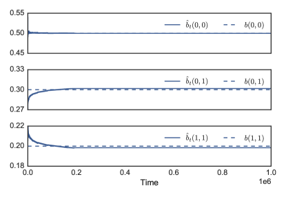
(a) Evolution of $\hat{b}_{t}$

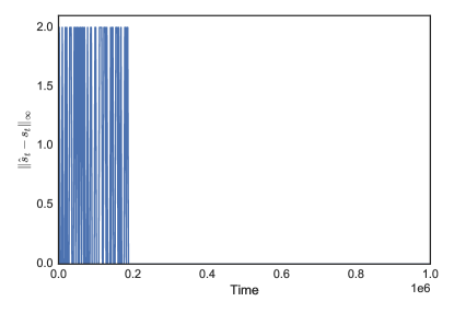
(b) Error in learned scheduling decisions

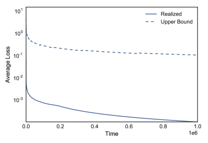
(c) Average realized loss

Figure 1: Output of Algorithm 2 for the example in Section 4

First note that Figure 1(a) shows that the $\hat{b}_{t}$ does not converge to $b$. We see that (to 4 decimal places)

$$\hat{b}_{T}=\left[\begin{array}[]{cc}0.4998&0.3018\\ {}\hfil&0.1984\end{array}\right]$$

and for the majority of the simulation these parameter estimates do not change. The reason is that (as shown in in Figure 1(b)) $\hat{b}_{T}$ yields the same scheduling decisions as $b$. The algorithm learns to emulate the expert scheduler so the loss becomes zero and the weights stop updating. This possibility was discussed at the beginning of Section 3.

Figure 1(c) which shows that while the average loss does indeed tend to zero, the upper bound proved in Theorem 2 is quite loose in this situation. This is expected due to the generality of the theorem. This also means that the concentration bound in Theorem 3 is quite conservative. Indeed, for this simulation we see that $f_{t}(\epsilon)=0$ for all $t$ and for any $\epsilon>0$. In other words, no observed loss ever exceeds the average case bound.

5 Extensions

We now discuss some extensions to our algorithms. We first note that we could replace line 14 in Algorithm 1 with

$$w_{t+1}\leftarrow w_{t}\cdot\exp(-\eta w_{t}).$$

The new algorithm would be a Hedge-style algorithm and we would be able to use apply other results (e.g. [5, Theorem 2.4]) to obtain similar upper bounds on the average loss.

We also note that we could modify our algorithms and obtain tighter upper bounds if we impose additional assumptions on the expert. For example, the expert may have a fairly simple objective that leads to prioritization of some queues over others. In this case, we would have $b(i,j)=0$ for $i\neq j$. Rather than having a triangular array of $p$ parameter estimates, we could instead keep track of just $n$ estimates. Since $\Theta(\ln(p))=\Theta(\ln(n))$, the convergence rate would not change but we would have smaller constant factors. Other sparsity patterns could be handled in a similar fashion. The diagonal case is slightly simpler because there would be no need use $\sigma(i,j)$ to keep track of the appropriate signs.

As noted in Section 2, a continuous-time PCS model with heterogenous and stochastic service times was considered in [3]. Our algorithms could be applied in this setting as well by updating the algorithm immediately after customer arrivals and departures rather than in discrete time slots. In [3], $B$ is diagonal and so we could apply the simplifications mentioned above. Our theorems would still hold because they not require that the state update happen at regularly spaced intervals – the algorithms merely require a stream of observed backlogs and observed scheduling actions.

6 Conclusions and Future Work

In this paper we have proposed an algorithm that learns a scheduling policy that emulates the behavior of an expert projective cone scheduler. This offers a data-driven way of designing automated scheduling policies that achieve the same goals as a human manager. We have provided several theoretical guarantees and have numerically demonstrated the efficacy of the algorithm on a simple example.

This paper opens the door for a few area of future work. One idea is to provide tighter bounds that depend on the statistical properties of the arrival process. A benefit of the current approach is that it does not require any assumptions on the arrival process but the clear downside is that the resulting bounds are quite loose. An algorithm that uses information about the arrival process could have faster convergence rates and tighter bounds.

Another idea is to investigate the impact of an approximate computation of $\mu$. As mentioned in Section 3, in large-scale problems, exactly computing $\mu(y;b)$ is generally a difficult problem and heuristic approaches are typically taken in practice. An area of future work would be to consider how such approximation “noise” affects our ability to emulate the expert scheduler.

References

References

- [1] N. Master, Z. Zhou, D. Miller, D. Scheinker, N. Bambos, P. Glynn, Improving predictions of pediatric surgical durations with supervised learning, International Journal of Data Science and Analytics (2017) 1–18.
- [2] C. Okoli, S. D. Pawlowski, The Delphi method as a research tool: an example, design considerations and applications, Information & management 42 (1) (2004) 15–29.
- [3] M. Armony, N. Bambos, Queueing dynamics and maximal throughput scheduling in switched processing systems, Queueing systems 44 (3) (2003) 209–252.
- [4] K. Ross, N. Bambos, Projective cone scheduling (PCS) algorithms for packet switches of maximal throughput, IEEE/ACM Transactions on Networking 17 (3) (2009) 976–989.
- [5] S. Arora, E. Hazan, S. Kale, The Multiplicative Weights Update Method: a Meta-Algorithm and Applications., Theory of Computing 8 (1) (2012) 121–164.
- [6] Y. Freund, R. E. Schapire, Adaptive game playing using multiplicative weights, Games and Economic Behavior 29 (1-2) (1999) 79–103.
- [7] S. A. Plotkin, D. B. Shmoys, É. Tardos, Fast approximation algorithms for fractional packing and covering problems, Mathematics of Operations Research 20 (2) (1995) 257–301.
- [8] A. Bärmann, S. Pokutta, O. Schneider, Emulating the Expert: Inverse Optimization through Online Learning, in: International Conference on Machine Learning, 2017, pp. 400–410.
- [9] M. D. Troutt, A. A. Brandyberry, C. Sohn, S. K. Tadisina, Linear programming system identification: The general nonnegative parameters case, European Journal of Operational Research 185 (1) (2008) 63–75.
- [10] A. Keshavarz, Y. Wang, S. Boyd, Imputing a convex objective function, in: IEEE International Symposium on Intelligent Control, IEEE, 2011, pp. 613–619.
- [11] J. Thai, A. M. Bayen, Imputing a variational inequality function or a convex objective function: A robust approach, Journal of Mathematical Analysis and Applications.
- [12] A. Y. Ng, S. J. Russell, Algorithms for inverse reinforcement learning., in: International Conference on Machine Learning, 2000, pp. 663–670.
- [13] P. Abbeel, A. Y. Ng, Apprenticeship learning via inverse reinforcement learning, in: International Conference on Machine learning, ACM, 2004, pp. 1–8.
- [14] K. Ross, N. Bambos, Local search scheduling algorithms for maximal throughput in packet switches, in: Annual Joint Conference of the IEEE Computer and Communications Societies (INFOCOM), Vol. 2, IEEE, 2004, pp. 1158–1169.