Spatiotemporal intermittency and localized dynamic fluctuations upon approaching the glass transition

Abstract

We introduce a new and robust method for characterizing spatially and temporally heterogeneous behavior within a system based on the evolution of dynamic fuctuations once averaged over different space lengths and time scales. We apply it to investigate the dynamics in two canonical systems as the glass transition is approached: a simulated Lennard-Jones glass-former and a real dense colloidal suspensions. We find that in both cases the onset of glassines is marked by spatially localized dynamic fluctuations originating in regions of correlated mobile particles. By removing the trivial system size dependence of the fluctuations we show that such regions contain tens to hundreds of particles for time scales corresponding to maximally non-Gaussian dynamics.

I Introduction

Glasses are solid materials with disordered liquid-like structure. These are typically formed by rapidly quenching a liquid from a hot to a cold temperature, or compressing a liquid from a low to a high pressure Angell (1995); Angell et al. (2000). How the transition from an equilibrium liquid to an out of equilibrium glass takes places is highly debated, with many different and contrasting interpretations proposed; see Refs. Langer (2014); Chandler and Garrahan (2010); Biroli and Garrahan (2013); Ediger and Harrowell (2012); Lubchenko and Wolynes (2007); Cavagna (2009) for reviews. One point is known: the onset of unusual behavior within a sample precedes the glass transition. “Supercooled liquids”, despite their metastable equilibrium, have a markedly higher viscosity $\eta$ than normal liquids. This step rise of $\eta$ is associate to the onset of dynamical heterogeneity: diffusive motion takes place in a spatially and temporally heterogeneous fashion Sillescu (1999); Ediger (2000); Glotzer (2000); Hempel et al. (2000); Richert (2002). At any given time, some regions within the sample are frozen, while other regions are quite mobile. The mobile regions are characterized by “cooperative” motion where localized groups of molecules have nearly simultaneous large displacements Glotzer (2000); Kob et al. (1997); Donati et al. (1998, 1999a). Over time, the locations of faster and slower dynamics change, such that at any given position the dynamics are temporally heterogeneous as well Chandler and Garrahan (2010); Garrahan and Chandler (2003); Keys et al. (2011).

In the last two decades, a variety of methods have been proposed and implemented to characterize such dynamical heterogeneities. Early work studied simulations of soft particles or Lennard-Jones particles and identified subsets of particles that had large displacements $\Delta r$ Hurley and Harrowell (1995, 1996); Kob et al. (1997); Donati et al. (1998, 1999a), showing that these formed spatially localized clusters. A key result was the identification of the non-Gaussian time scale $\Delta t^{*}$ as an important time scale related to these clusters Hurley and Harrowell (1996); Kob et al. (1997); Marcus et al. (1999). This time scale is identified by examining the behavior of the non-Gaussian parameter $\alpha_{2}(\Delta t)=3\langle\Delta r^{4}\rangle/(5\langle\Delta r^{2}\rangle^{2})-1$, a quantity derived from the moments of the displacement distribution $P(\Delta r)$ Rahman (1964). $\Delta t^{*}$ is the time scale for which $\alpha_{2}(\Delta t)$ is maximal. $\alpha_{2}$ is zero when $P(\Delta r)$ is a Gaussian, which holds to a good approximation for simple liquids. For dynamically heterogeneous supercooled liquids, $\alpha_{2}>0$ indicating that particles with large displacements occur more frequently than would occur for a Gaussian distribution. Identifying the particles responsible for the large $\alpha_{2}$ value is expected to provide information on the cooperatively moving clusters Kob et al. (1997); Donati et al. (1998, 1999a) and their structural and dynamic properties. Early studies Kob et al. (1997); Donati et al. (1998, 1999a) used various somewhat arbitrary criteria to define mobile particles. Later work examined spatial correlation functions averaged over all particles in various ways attempting to identify the length and time scales of dynamical heterogeneity Donati et al. (1999a); Flenner and Szamel (2007); Doliwa and Heuer (2000); Weeks et al. (2007); Glotzer (2000); Lačević et al. (2003); Keys et al. (2007); Appignanesi et al. (2006); Appignanesi and Rodriguez Fris (2009).

In this manuscript, we present a new and robust analysis method to characterize spatial and temporal dynamical heterogeneity that does not requires any a priori definition of particle mobility. In particular, we here use the system mean square displacement as a “null hypothesis” for particle motion, and quantify spatially and temporally localized deviations of particle motion away from this null hypothesis. We apply this method to the Kob-Andersen Lennard-Jones glassforming system Kob and Andersen (1995) and to colloidal supercooled liquid data Weeks et al. (2000). Our results show that dynamical heterogeneity is most obvious for subsystems comprised of tens to hundreds of particles, with the size growing as the glass transition is approached. Additionally, we examine how dynamical heterogeneity becomes averaged out at larger length scales. As a byproduct we confirm that $\Delta t^{*}$ is the time scale of maximum heterogeneity. While our method of localized fluctuations is applied to particle displacements, the idea is generalizable to other quantities which may have spatiotemporal fluctuations such as structure Royall and Williams (2015); Royall et al. (2008). An advantage of our technique is that it is applicable to small data sets such as the experimental colloidal data we use.

II Simulation and Experimental Details

II.1 Simulation

We use LAMMPS to simulate the Kob-Andersen binary Lennard-Jones glassforming system Kob and Andersen (1995). Briefly, this is an 80:20 mixture of $A$ and $B$ particles. The particles interact via the Lennard-Jones potential Lennard-Jones (1924)

$$U_{\alpha\beta}(r)=4\epsilon_{\alpha\beta}\left[\left(\frac{\sigma_{\alpha\beta}}{r}\right)^{12}-\left(\frac{\sigma_{\alpha\beta}}{r}\right)^{6}\right]$$ (1)

with $\alpha,\beta\in{A,B}$. $A$ and $B$ particles have the same mass. The energy scales are $\epsilon_{AA}=1.0$, $\epsilon_{AB}=1.5$, and $\epsilon{BB}=0.5$. The size scales are $\sigma_{AA}=1.0$, $\sigma_{AB}=0.8$, and $\sigma_{BB}=0.88$, chosen so that $A$ and $B$ particles are encouraged to mix rather than segregate, and thus crystallization is frustrated Kob and Andersen (1995). For most of our results we present data with 8000 total particles, and for our analysis we consider the $N=6400$ $A$ particles. To verify that our analysis is not biased by finite size, in a few cases we compare with a $N=8\times 10^{5}$ data set. Periodic boundary conditions were used with a cubical box.

II.2 Experiment

Colloids have long been used as model systems to study the glass transition Hunter and Weeks (2012); Marshall and Zukoski (1990); Pusey and van Megen (1987, 1986); Härtl (2001); van Megen and Pusey (1991); Bartsch et al. (1993); Meller and Stavans (1992); Lindsay and Chaikin (1982). We reanalyze previously published data from experiments using confocal microscopy to observe dense colloidal samples Weeks et al. (2000). The samples were sterically stabilized colloidal poly-(methyl methacrylate) for which the key control parameter is the volume fraction $\phi$ Hunter and Weeks (2012). The glass transition for this experiment occurred at $\phi_{g}=0.58$. Here we examine data with $\phi=0.46,0.52,0.56$ with $N\approx 2500,2900,3100$ particles respectively in the observation volume. The particles were a single species with mean particle diameter 2.36 $\mu$m and a polydispersity of 0.045 Kurita et al. (2012) and were slightly charged. Confocal microscopy and particle tracking was used to follow the positions of the particles in three dimensions Dinsmore et al. (2001); Crocker and Grier (1996). The imaging volume was rectangular with an aspect ratio roughly $5:5:1$; see Ref. Weeks et al. (2000) for details.

III Results

We aim at characterizing the growing spatial and temporal fluctuations on approaching the glass transition without introducing any arbitrary cut-off quantity. Following prior work Ohmine and Tanaka (1993); Appignanesi et al. (2006); Appignanesi and Rodriguez Fris (2009), we start by defining the distance matrix $\Delta^{2}(t^{\prime},t^{\prime\prime})$, an object that represents the average of the squared particle displacements between time $t^{\prime}$ and $t^{\prime\prime}$ of a collection of the $N$ particles belonging to a predefined set $S$ ($S$ may be the entire system or some subsystem):

$$\Delta^{2}(t^{\prime},t^{\prime\prime}) \equiv \frac{1}{N}\sum_{i=1}^{N}|\vec{r}_{i}(t^{\prime})-\vec{r}_{i}(t^{\prime\prime})|^{2}$$ (2)

$$= \langle|\vec{r}_{i}(t^{\prime})-\vec{r}_{i}(t^{\prime\prime})|^{2}\rangle_{i\in S}$$ (3)

where the angle brackets indicate an average over the $N$ particles in $S$. Further averaging $\Delta^{2}(t^{\prime},t^{\prime\prime})$ over all pairs $t^{\prime}$ and $t^{\prime\prime}$ such that $t^{\prime\prime}-t^{\prime}=\Delta t$ produces the well-known average mean square displacement $M^{2}(\Delta t)$ of particles in $S$. More precisely

$$M^{2}(\Delta t)=\langle\Delta^{2}(t^{\prime},t^{\prime\prime})\rangle_{t^{\prime\prime}-t^{\prime}=\Delta t}$$ (4)

where the average is over $t^{\prime},t^{\prime\prime}$ with fixed time interval $\Delta t=|t^{\prime\prime}-t^{\prime}|$ and also over all of the particles in $S$. Assuming stationary dynamics (true as long as the system is not aging), for a sufficiently large $\Delta t$, $\lim_{\Delta t\rightarrow\infty}\Delta^{2}(t^{\prime},t^{\prime}+\Delta t)=M^{2}(\Delta t)$

For small systems under glassy relaxation conditions, $\Delta^{2}$ has temporal fluctuations, as shown in Fig. 1(a) for a sub-system of $N=125$ particles. Darker regions indicate time intervals $(t^{\prime},t^{\prime\prime})$ over which this subsystem has relatively little particle motion. Clearly, there are specific times for which this subsystem undergoes fairly large changes, signalled by larger displacements and substantially different particle positions. It is expected La Nave and Sciortino (2004) than on increasing the sample size well beyond any dynamic correlation length, different regions of the system will independently display such burst motion, such that $\Delta^{2}$ for larger systems will appear much smoother, as shown in Fig. 1(b) for the fully system of $N=8000$ particles. As for the long time limit, for a sufficiently large system $S$, $\lim_{N\rightarrow\infty}\Delta^{2}(t^{\prime},t^{\prime}+\Delta t)=M^{2}(\Delta t)$

Figure 1: (a) Contour plot of the distance matrix $\Delta^{2}(t^{\prime},t^{\prime\prime})$ for a binary Lennard-Jones system at $T=0.50$ within a cubical subsystem containing 125 particles. The legend indicates the values of the gray scale. (b) Contour plot of the same system for the full 8000 particle simulation. Images taken from Ref. Appignanesi and Rodriguez Fris (2009), permission pending. (c) $\Omega(t^{\prime},t^{\prime\prime})$. The data correspond to the same subsystem as in (a). In the image shown, darker points indicate larger values. (d) The values of $\Delta^{2}$ as a function of $\Delta t=|t^{\prime}-t^{\prime\prime}|$ for the data shown in (a). For small $\Delta t$ this tends to 0, and for intermediate $\Delta t$ the scatter indicates the temporal heterogeneity in this subsystem. The overall increase mirrors the mean square displacement $M^{2}(\Delta t)$. (e) $\Omega^{2}(\Delta t)$ for the data shown in (c). The scatter at small $\Delta t$ reflects a function of $\Delta t$, which has much larger fluctuations at short $\Delta t$, reflecting non-Gaussian statistics of the displacements at those time scales.

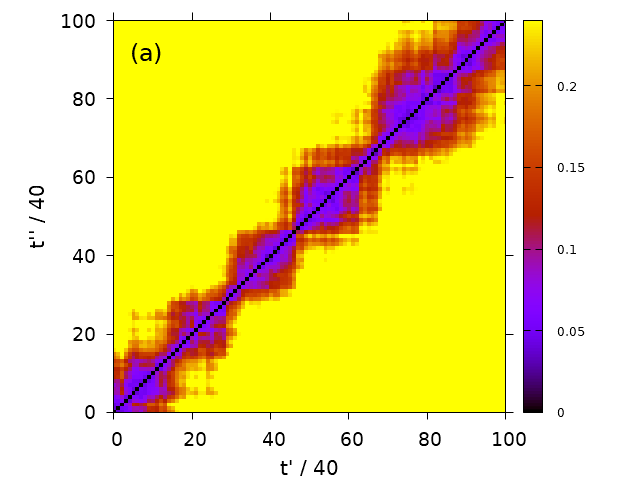
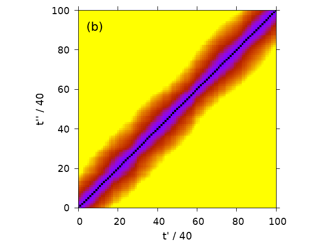
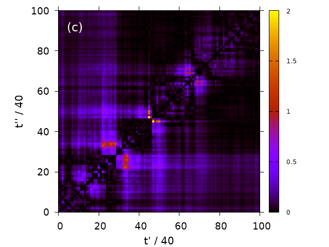
The question we turn to is how the large system limit is reached. In particular, we wish to use the approach to the large system limit to characterize the spatial scale of dynamical heterogeneities. The obvious features of Fig. 1(a) are the large fluctuations that differentiate it from Fig. 1(b). This motivates us to consider the normalized difference between $\Delta^{2}$ and the expectation for a large system, defined by

$$\Omega_{S}^{2}(t^{\prime},t^{\prime\prime})=\frac{[\Delta^{2}(t^{\prime},t^{\prime\prime})-M^{2}(\Delta t)]^{2}}{[M^{2}(\Delta t)]^{2}}$$ (5)

with the convention $\Delta t=|t^{\prime\prime}-t^{\prime}|$. $\Omega_{S}^{2}$, a measure of the dynamic intermittency, represents the matrix of normalized squared deviations from the mean value for the particles squared displacements and will be equal to zero when $\Delta^{2}$ is calculated for sufficiently large systems, for which time averages and space averages are equivalent and $\Delta^{2}=M^{2}$. Otherwise, $\Omega_{S}^{2}>0$ and larger values indicate larger deviations between $\Delta^{2}$ (local in both space and time) and the expectation for a large system (that is, $M^{2}$, a quantity averaged over all space and all time).

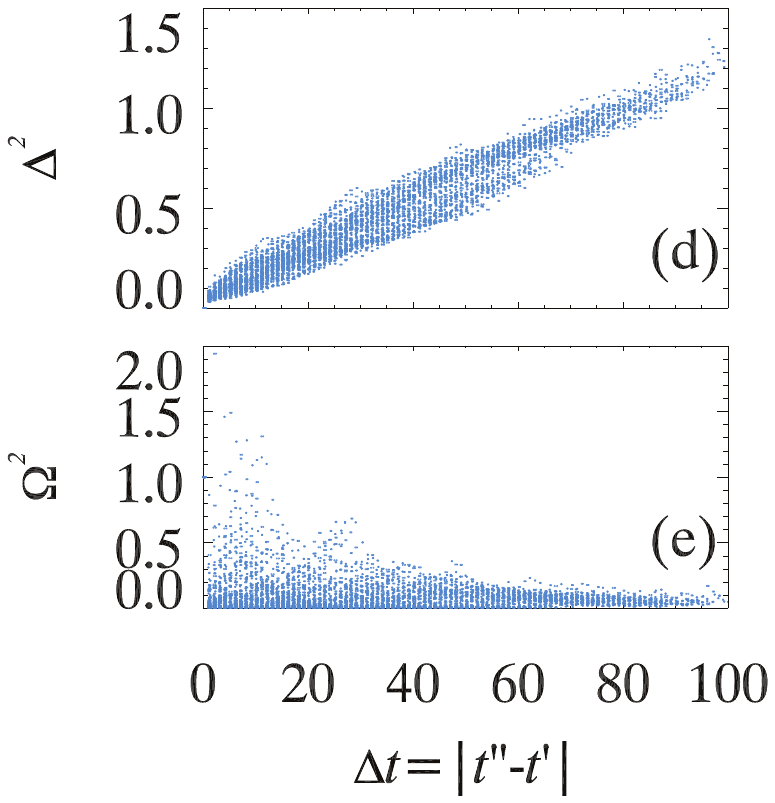
An example of $\Omega^{2}_{S}(t^{\prime},t^{\prime\prime})$ is shown in Fig. 1(c), where the darker regions indicate time periods for which the mean motion within the sub-volume is anomalously larger or smaller compared to the expectation from $M^{2}$. Fig. 1(d) and 1(e) show scatter plots of the values of $\Delta^{2}$ and $\Omega_{S}^{2}$ as functions of $t^{\prime\prime}-t^{\prime}$, taken from the data of Fig. 1(a) and 1(c) respectively. $\Delta^{2}$ starts at the origin and rises, consistent with the idea that on average it should behave similar to the mean square displacement $M^{2}(\Delta t)$. At intermediate time scales the scatter in the data of Fig. 1(d) indicates the temporal fluctuations of the motion. In contrast, $\Omega_{S}^{2}$ in Fig. 1(e) has large fluctuations at the shortest time scales, indicating large fluctuations of the motion relative to $M^{2}(\Delta t)$ on those time scales. At larger time scales, the temporal averaging reduces $\Omega_{S}^{2}$ toward zero.

As defined, $\Omega^{2}_{S}$ is local in space and time. To focus on the space dependence of the fluctuations we need to evaluate a single nondimensional scalar quantity $\Omega(N)$ characterizing the mobility fluctuations for subsystems of size $N$ (the ratio of the dispersion to the average Chandler (1987) for the particle squared displacements). To do so we partition the system into distinct cubical boxes containing $N$ particles each and evaluate the sum of $\Omega_{S}^{2}(t^{\prime},t^{\prime\prime})$ over all time pairs ($t^{\prime}$, $t^{\prime\prime}$) [i.e. the sum over all points entering in the scatter-plot as the one shown in Fig. 1(e)] divided by the number of such pairs for each of the boxes. We then average the resulting number over all boxes and finally take the square root of the result. This procedure yields the desired scalar quantity $\Omega(N)$. Note that the specific values of $\Omega(N)$ will depend on the total time studied, that is, the maximum of $|t^{\prime\prime}-t^{\prime}|$ that is studied. As is apparent from Fig. 1(c) and 1(e), at large $|t^{\prime\prime}-t^{\prime}|$, $\Omega_{S}$ decays to zero, and the more of this included in the average, the smaller $\Omega(N)$ will be. However, for a given data set, what will matter is the $N$-dependence which is insensitive to the total time studied, as long as that time is sufficient to capture the temporal fluctuations seen in Fig. 1(c). In practice, we ensure that our data sets have a total duration of $\approx 10\Delta t^{*}$ where $\Delta t^{*}$ depends on the temperature (for the Lennard-Jones simulations) or the volume fraction (for the colloidal experiments). This then will allow for a sensible comparison between different data sets.

Figure 2: $\Omega({\rm N})$ and $\Omega_{R}({\rm N})$ as a function of subsystem size $N$ for the binary Lennard-Jones system [(a) and (c)] for different temperatures as indicated and for the experimental colloidal suspension [(b) and (d)] at different volume fractions $\phi$ as indicated. In the case of $\Omega({\rm N})$ the $N$ particles are part of the same subsystem. In the case of $\Omega_{R}({\rm N})$ the $N$ particles are selected randomly among all particles in the system.

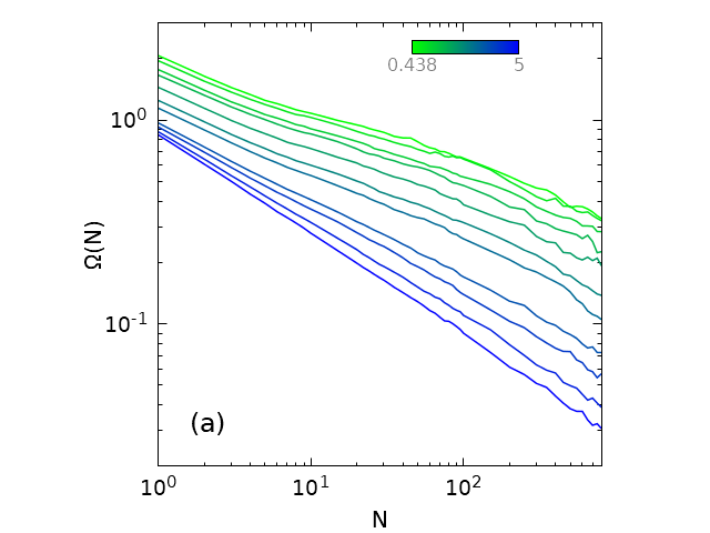
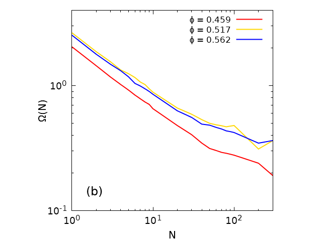
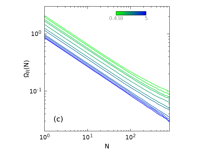
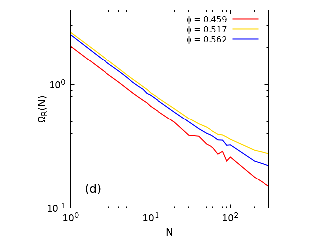
$\Omega(N)$ for the Lennard-Jones system is plotted in Fig. 2(a), and for the colloidal experiments in Fig. 2(b). In both cases, we see how the dynamical fluctuations average out for larger subsystem sizes. Notably, the systems closer to the glass transition require larger subsystems before the dynamical fluctuations are averaged out – colder systems for the LJ data (a), and higher volume fraction systems for the colloidal data (b).

Figure 3: Subtracting $\Omega$ calculated for randomly chosen particles from $\Omega$ calculated for compact subsystems. (a) For the LJ system; (b) for the colloidal suspensions. The black curve in (a) shows the same quantity evaluate for a system of 1M particles at $T=0.466$, showing that the position of the maximum is not affected by the finite size of the investigated system.

An interesting point emerges when analyzing the functional form of the decay of $\Omega(N)$ with $N$. From the high temperature data of Fig. 2(a) we observe the spatially localized dynamic fluctuations measured by $\Omega$ display the usual $N^{-1/2}$ size scaling dependence. This reflects that particle motion is nearly spatially uncorrelated within a subsystem and so the average of $\Delta^{2}(N)$ converges to the large-system limit $M^{2}$ as $N^{-1/2}$. However, for glassier systems a clear departure from this trivial behavior is seen, and the decay of $\Omega(N)$ gets slower. The fact that the localized dynamical fluctuations are higher than expected, persisting at large system sizes, speaks of the existence of regions of correlated mobile particles, an effect that is more pronounced upon supercooling Glotzer (2000); Kob et al. (1997); Donati et al. (1998, 1999a); Weeks et al. (2000, 2007). We truncate our calculation at $N=N_{max}/10$, as we desire at least 10 subsystems to evaluate a reasonable $\Omega(N)$. We note that both for the Lennard-Jones system and the colloidal suspensions, the behavior of the curves of Fig. 2 at very large system sizes is due to lack of statistics (the subsystems are not small as compared to the large system and, thus, we can only average over a few of them).

As evident from Fig. 2, for the smallest possible subsystems ($N=1$), the increasing value of $\Omega$ as the glass transition is approached reflects the well-known increasing non-Gaussian nature of the displacement distribution Kob and Andersen (1995). In fact this points out a limitation of $\Omega$, in that large values of $\Omega$ can reflect either spatial fluctuations in the dynamics or simply a non-Gaussian distribution of displacements. To remove the latter influence (that is, to remove the trivial system size dependence and thus to highlight the local correlations) we separately compute $\Omega_{R}(N)$ based not on compact subsystems of size $N$ but on $N$ randomly chosen particles. Here the subscript $R$ indicates an average over many such randomly chosen subsets. For the Lennard-Jones system, this is plotted in Fig. 2(c), showing different behavior from Fig. 2(a) for the colder temperature data. In fact, now the randomly distributed dynamical fluctuations quantified by $\Omega_{R}(S)$ display the typical $N^{-1/2}$ decay at all temperatures. Similar behavior is found in Fig. 2(d) for the colloidal suspensions, as compared to Fig. 2(b). Again, the $N^{-1/2}$ scaling is recovered at all volume fractions.

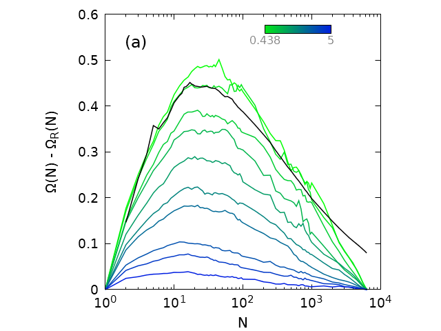
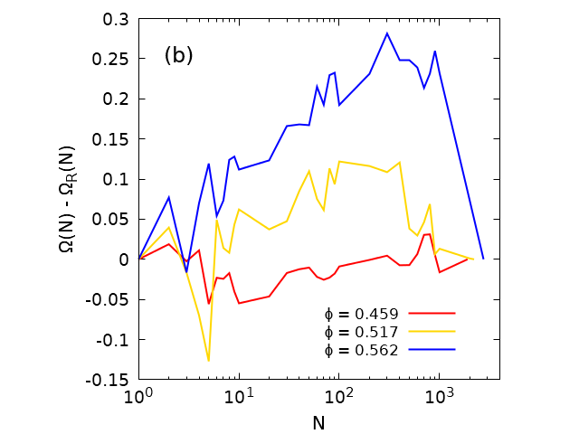
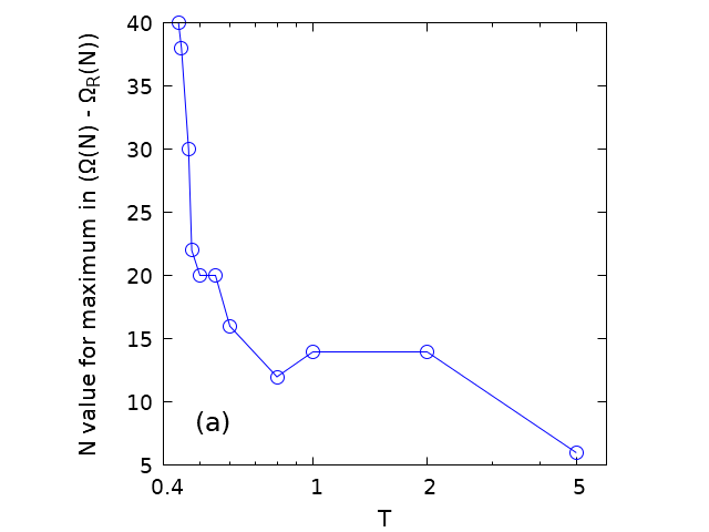
To understand the differences between the spatially localized and the randomly distributed dynamic fluctuations, in Fig. 3(a) we show the result of subtracting $\Omega_{R}(N)$ from $\Omega(N)$. For $N=1$ particles the result is zero as there is no distinction between the two calculations. Likewise for $N\rightarrow 6400$ (the total number of $A$ particles), the two calculations are identical. At intermediate numbers of particles, nonzero values are found in Fig. 3(a) indicating nontrivial spatially localized values of $\Omega$. In particular, for colder temperatures the dynamical fluctuations are larger [higher curves in Fig. 3(a)] and the subsystem size with the largest fluctuations grows slightly [peak position shifts rightward in Fig. 3(a)]. This last observation is quantified in Fig. 4 which shows the peak position of Fig. 3(a) as a function of $T$. The peak occurs for larger subsystems at colder temperatures. This indicates the size of regions with maximally variable dynamics contain about 50 particles for the coldest samples. For hotter samples, the maximum shifts to smaller system sizes; for the hottest data, $\Omega$ for compact subsystems is nearly indistinguishable from $\Omega$ calculated for random particles, and we cannot identify a maximum. In turn, Fig. 3(b) shows the behavior for the colloidal suspensions, which is similar to that found for the Lennard-Jones system. Namely, there is a peak in Fig. 3(b) at a specific subsystem size, and the position and height of this peak is larger for volume fractions closer to the glass transition volume fraction ($\phi_{\rm g}\approx 0.58$ Weeks et al. (2000)). An intriguing difference is that the peak position indicates that larger subsystems containing a few hundred particles are maximally heterogeneous, as compared to Fig. 3(a) which peaks at subsystem sizes containing a few tens of particles. Earlier work with the Lennard-Jones system found mobile clusters containing 10-30 particles Donati et al. (1999b) or 40 particles Appignanesi et al. (2006) at the coldest temperatures, in agreement with our result. Likewise, earlier analyses of the same colloidal data found the largest mobile clusters contained $\sim 50$ particles on average for $\phi=0.562$ Weeks et al. (2000). The new result seen here is how the sample behaves over larger length scales. For example, Fig. 3(a) shows that there is still nontrivial spatial heterogeneity for subsystems containing $N=1000$ particles, more than an order of magnitude larger than the $N$ corresponding to the peak. This is strong evidence that the dynamically heterogeneous regions of size $N\sim 50$ are not randomly distributed throughout the sample but are themselves spatially clustered.

Figure 4: (a) Value of $N$ that maximizes $\Omega(N)$ in Fig. 3(a) as a function of $T$. (b) Comparison of the time scale of the maxima from Fig. 3(a) with the time scale $\Delta t^{*}$.

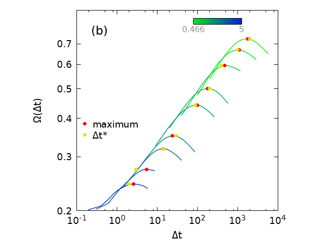
In the preceding analysis, $\Omega^{2}_{S}$ is averaged over time scales to highlight the $N$ dependence of the dynamical fluctuations. We now turn to the complementary case, and average $\Omega^{2}_{S}$ over subsystem sizes $N$ to find the time scale $\Delta t$ of the same fluctuations. Since the value of $N$ covers several order of magnitude, we average $\Omega_{S}(t^{\prime},t^{\prime\prime})$ over subsystems with sizes $N$ picked to be evenly distributed in $\log(N)$, with $N$ ranging from 1 to the system size. We first average over all subsystems of a given size $N$, and then average $\Omega^{2}(N,t^{\prime},t^{\prime\prime})$ over $N$ and $(t^{\prime},t^{\prime\prime})$ with fixed time interval $\Delta t=t^{\prime\prime}-t^{\prime}$ to result in $\Omega(\Delta t)$. This is shown in Fig. 4(b) where the peak of each curve is marked with a red circle. For comparison, the time scale $\Delta t^{*}$ is indicated for each data set with a yellow circle; it appears the peak of $\Omega(\Delta t)$ is always close to the non-Gaussian time scale $\Delta t^{*}$. As expected, the time scale of maximum dynamical heterogeneity [as measured by $\Omega(\Delta t)$] grows as the system approaches the glass transition.

IV Conclusions

In summary, we have constructed a new measure of spatial and temporal dynamic heterogeneity. The measure does not require defining subsets of mobile or immobile particles, but rather looks for fluctuations away from the large system behavior. Additionally, it allows us to examine dynamical heterogeneity on a variety of length scales, showing that the approach to the large system limit is slower than would be expected for randomly distributed fluctuations in the dynamics. The method can be straightforwardly applied to experimental systems such as the dense colloidal solution we examine; it does not require finite-size scaling, for example. While we focus on particle motion where the mean square displacement is the null hypothesis, the method can be generalized to any other spatially and temporally fluctuating quantities, as long as there is a well-defined null hypothesis based on the large system limit.

The work of E.R.W was supported by a grant from the National Science Foundation (DMR-1609763). GAA and JARF acknowledge suport form CONICET, UNS and ANPCyT(PICT2015/1893). Inspiration for this work came from past conversations with Prof. Walter Kob.

References

- Angell (1995) C. A. Angell, Science 267, 1924 (1995).
- Angell et al. (2000) C. A. Angell, K. L. Ngai, G. B. McKenna, P. F. McMillan, and S. W. Martin, J. App. Phys. 88, 3113 (2000).
- Langer (2014) J. S. Langer, Rep. Prog. Phys. 77, 042501 (2014).
- Chandler and Garrahan (2010) D. Chandler and J. P. Garrahan, Ann. Rev. Phys. Chem. 61, 191 (2010).
- Biroli and Garrahan (2013) G. Biroli and J. P. Garrahan, J. Chem. Phys. 138, 12A301 (2013).
- Ediger and Harrowell (2012) M. D. Ediger and P. Harrowell, J. Chem. Phys. 137, 080901 (2012).
- Lubchenko and Wolynes (2007) V. Lubchenko and P. G. Wolynes, Ann. Rev. Phys. Chem. 58, 235 (2007).
- Cavagna (2009) A. Cavagna, Phys. Rep. 476, 51 (2009).
- Sillescu (1999) H. Sillescu, J. Non-Cryst. Solids 243, 81 (1999).
- Ediger (2000) M. D. Ediger, Ann. Rev. Phys. Chem. 51, 99 (2000).
- Glotzer (2000) S. C. Glotzer, Physics of Non-Crystalline Solids 9, J. Non-Cryst. Solids 274, 342 (2000).
- Hempel et al. (2000) E. Hempel, G. Hempel, A. Hensel, C. Schick, and E. Donth, J. Phys. Chem. B 104, 2460 (2000).
- Richert (2002) R. Richert, J. Phys.: Condens. Matter 14, R703 (2002).
- Kob et al. (1997) W. Kob, C. Donati, S. J. Plimpton, P. H. Poole, and S. C. Glotzer, Phys. Rev. Lett. 79, 2827 (1997).
- Donati et al. (1998) C. Donati, J. F. Douglas, W. Kob, S. J. Plimpton, P. H. Poole, and S. C. Glotzer, Phys. Rev. Lett. 80, 2338 (1998).
- Donati et al. (1999a) C. Donati, S. C. Glotzer, and P. H. Poole, Phys. Rev. Lett. 82, 5064 (1999a).
- Garrahan and Chandler (2003) J. P. Garrahan and D. Chandler, Proc. Nat. Acad. Sci. 100, 9710 (2003).
- Keys et al. (2011) A. S. Keys, L. O. Hedges, J. P. Garrahan, S. C. Glotzer, and D. Chandler, Phys. Rev. X 1, 021013 (2011).
- Hurley and Harrowell (1995) M. M. Hurley and P. Harrowell, Phys. Rev. E 52, 1694 (1995).
- Hurley and Harrowell (1996) M. M. Hurley and P. Harrowell, J. Chem. Phys. 105, 10521 (1996).
- Marcus et al. (1999) A. H. Marcus, J. Schofield, and S. A. Rice, Phys. Rev. E 60, 5725 (1999).
- Rahman (1964) A. Rahman, Phys. Rev. 136, A405 (1964).
- Flenner and Szamel (2007) E. Flenner and G. Szamel, J. Phys.: Condens. Matter 19, 205125 (2007).
- Doliwa and Heuer (2000) B. Doliwa and A. Heuer, Phys. Rev. E 61, 6898 (2000).
- Weeks et al. (2007) E. R. Weeks, J. C. Crocker, and D. A. Weitz, J. Phys.: Condens. Matter 19, 205131 (2007).
- Lačević et al. (2003) N. Lačević, F. W. Starr, T. B. Schrøder, and S. C. Glotzer, J. Chem. Phys. 119, 7372 (2003).
- Keys et al. (2007) A. S. Keys, A. R. Abate, S. C. Glotzer, and D. J. Durian, Nature Phys. 3, 260 (2007).
- Appignanesi et al. (2006) G. A. Appignanesi, J. A. Rodriguez Fris, R. A. Montani, and W. Kob, Phys. Rev. Lett. 96, 057801 (2006).
- Appignanesi and Rodriguez Fris (2009) G. A. Appignanesi and J. A. Rodriguez Fris, J. Phys.: Condens. Matter 21, 203103 (2009).
- Kob and Andersen (1995) W. Kob and H. C. Andersen, Phys. Rev. E 51, 4626 (1995).
- Weeks et al. (2000) E. R. Weeks, J. C. Crocker, A. C. Levitt, A. Schofield, and D. A. Weitz, Science 287, 627 (2000).
- Royall and Williams (2015) C. P. Royall and S. R. Williams, Phys. Rep. 560, 1 (2015).
- Royall et al. (2008) C. P. Royall, S. R. Williams, T. Ohtsuka, and H. Tanaka, Nat Mater 7, 556 (2008).
- Lennard-Jones (1924) J. E. Lennard-Jones, Proc. Roy. Soc. London A: Mathematical, Physical and Engineering Sciences 106, 463 (1924).
- Hunter and Weeks (2012) G. L. Hunter and E. R. Weeks, Rep. Prog. Phys. 75, 066501 (2012).
- Marshall and Zukoski (1990) L. Marshall and C. F. Zukoski, J. Phys. Chem. 94, 1164 (1990).
- Pusey and van Megen (1987) P. N. Pusey and W. van Megen, Phys. Rev. Lett. 59, 2083 (1987).
- Pusey and van Megen (1986) P. N. Pusey and W. van Megen, Nature 320, 340 (1986).
- Härtl (2001) W. Härtl, Curr. Op. Coll. Int. Sci. 6, 479 (2001).
- van Megen and Pusey (1991) W. van Megen and P. N. Pusey, Phys. Rev. A 43, 5429 (1991).
- Bartsch et al. (1993) E. Bartsch, V. Frenz, S. Moller, and H. Sillescu, Physica A 201, 363 (1993).
- Meller and Stavans (1992) A. Meller and J. Stavans, Phys. Rev. Lett. 68, 3646 (1992).
- Lindsay and Chaikin (1982) H. M. Lindsay and P. M. Chaikin, J. Chem. Phys. 76, 3774 (1982).
- Kurita et al. (2012) R. Kurita, D. B. Ruffner, and E. R. Weeks, Nature Comm. 3, 1127 (2012).
- Dinsmore et al. (2001) A. D. Dinsmore, E. R. Weeks, V. Prasad, A. C. Levitt, and D. A. Weitz, App. Optics 40, 4152 (2001).
- Crocker and Grier (1996) J. C. Crocker and D. G. Grier, J. Colloid Interface Sci. 179, 298 (1996).
- Ohmine and Tanaka (1993) I. Ohmine and H. Tanaka, Chem. Reviews 93, 2545 (1993).
- La Nave and Sciortino (2004) E. La Nave and F. Sciortino, J. Phys. Chem. B 108, 19663 (2004).
- Chandler (1987) D. Chandler, Introduction to Modern Statistical Mechanics, by David Chandler, pp. 288. Oxford University Press, Sep 1987. , 288 (1987).
- Donati et al. (1999b) C. Donati, S. C. Glotzer, P. H. Poole, W. Kob, and S. J. Plimpton, Phys. Rev. E 60, 3107 (1999b).