ExoCross: a general program for generating spectra from molecular line lists

ExoCross is a Fortran code for generating spectra (emission, absorption) and thermodynamic properties (partition function, specific heat etc.) from molecular line lists. Input is taken in several formats, including ExoMol and HITRAN formats. ExoCross is efficiently parallelized showing also a high degree of vectorization. It can work with several line profiles such as Doppler, Lorentzian and Voigt and support several broadening schemes. Voigt profiles are handled by several methods allowing fast and accurate simulations. Two of these methods are new. ExoCross is also capable of working with the recently proposed method of super-lines. It supports calculations of lifetimes, cooling functions, specific heats and other properties. ExoCross can be used to convert between different formats, such as HITRAN, ExoMol and Phoenix. It is capable of simulating non-LTE spectra using a simple two-temperature approach. Different electronic, vibronic or vibrational bands can be simulated separately using an efficient filtering scheme based on the quantum numbers.

1 Introduction

We present a Fortran 2003 program ExoCross to compute spectra as well as spectral properties of molecules using line lists. ExoCross is specifically developed to work with huge molecular line lists such as those generated as part of our ExoMol project (Tennyson & Yurchenko, 2012) or similar endeavours (Rey et al., 2016). ExoCross takes such line lists as input and returns pressure- and temperature-dependent cross sections as well a variety of other derived molecular properties which depend on the underlying spectroscopic data. These include state-dependent lifetimes, temperature-dependent cooling functions, and thermodynamic properties such as partition functions and specific heats.

The main challenge when working with hot line lists for polyatomic molecules is their extremely large sizes. Thus, for example, there are several line lists generated as part of the ExoMol project containing in excess of 10 billion transitions (Yurchenko & Tennyson, 2014; Sousa-Silva et al., 2015; Underwood et al., 2016a; Yurchenko et al., 2017a; Owens et al., 2017; Pavlyuchko et al., 2015; Al-Refaie et al., 2015b, a; Yurchenko et al., 2017a). The size of these datasets makes them impractical for direct use in line-by-line applications. We note that simply ignoring the billions of often very weak lines does not give reliable results (Yurchenko et al., 2014, 2017a). While there are a number of approaches to this problem such as the use of $k$-coefficients (see, for example, Showman et al. (2009); Amundsen et al. (2014); Malik et al. (2017); Min (2017)), the most practical approach which does not involve making significant approximations is to produce cross sections for a set of predefined conditions. These cross sections are then easier to handle in, for example, radiative transfer codes than the original line lists as they can be stored on far fewer grid points than there are lines. However handling these large line lists requires care and, in particular, the generation of cross sections on an appropriate temperature-, pressure- and frequency/wavelength-dependent grid is data intensive and can become computationally highly demanding. ExoCross provides a computational solution to this problem; it has been extensively optimised to process huge datasets, including the introduction of an efficient algorithm for generation large numbers of Voigt profiles which is discussed below. ExoCross is optimized to provide high throughput via efficient parallelization and vectorization. This is especially important when working with line lists containing tens of billions lines. At different stages of development ExoCross was used to generate spectra by Underwood et al. (2016b, a); McKemmish et al. (2016); Wong et al. (2017); Tennyson & Yurchenko (2017); Yurchenko et al. (2017a); Owens et al. (2017); Prajapat et al. (2017); Yurchenko et al. (2018) and Rutkowski et al. (2018).

ExoCross is designed to generate molecular cross sections (absorption or emission) on a grid for a set of temperatures and pressures using different line profiles (e.g. Doppler, Voigt etc) under the local thermodynamic equilibrium (LTE) as well as non-LTE (Darby-Lewis et al., 2018). Other useful functionality include computing lifetimes (Tennyson et al., 2016a), stick spectra, partition functions, cooling functions, and specific heats. The HITRAN molecular spectroscopic database (Gordon et al., 2017) is a widely-used compilation aimed at radiative transport studies of the Earth’s atmosphere. ExoCross is capable of working with HITRAN line lists (.par) as well as super-lines (Rey et al., 2016; Yurchenko et al., 2017a). It can be easily extended to accept other formats.

As part of this implementation, we have developed two new algorithms to perform convolution integrals needed for the Voigt line profile. The first algorithm is based on the Gauss-Hermite quadratures and is developed specifically to guarantee conservation of the Voigt line area. The second algorithm is based on exploiting the similarity of the Voigt profile at large distances from the line centre to compute the opacities quickly.

There are a number of other similar programs available which are designed to work with line lists. These include the HITRAN interface HAPI (Kochanov et al., 2016), SpectraPlot.com (Goldenstein et al., 2017) and SPECTRA (Tennyson et al., 1993). However, all of these programs would struggle to handle the huge line lists required for models of atmospheres at elevated temperatures. ExoCross is designed to be flexible; it takes input in both ExoMol (Tennyson et al., 2013, 2016b) and HITRAN (Rothman et al., 2005) formats. Data can be returned in a variety of formats: ExoMol, HITRAN and Phoenix (Jack et al., 2009), where Phoenix is a full non-LTE atmospheric transfer code accounting for depth-dependent abundances (cloud formation, element diffusion, etc.) using the line-by-line approach. Thus as a subsidiary function the code can be used to interconvert between ExoMol and HITRAN formats.

The paper is organised as follows. The main functionality of ExoCross is presented in Section 2. The line profile implemented in ExoCross are discussed in Section 3. Section 4 presents ExoCross calculation steps. The data format are described in Section 5. Section 7 offers some conclusions. The ExoCross manual provided as part of the supplementary data as well as GitHub and CCPForge repositories gives full working details of the program so the description below is restricted to outlines and examples.

2 Main functionality

2.1 Intensities and partition function

An absorption line intensity $I_{\rm fi}$ (cm/molecule), also known as absorption coefficient, is given by

$$I({\rm f}\leftarrow{\rm i})=\frac{g_{f}^{\rm tot}A_{\rm fi}}{8\pi c\tilde{\nu}_{\rm fi}^{2}}\frac{e^{-c_{2}\tilde{E}_{i}/T}\left(1-e^{-c_{2}\tilde{\nu}_{\rm fi}/T}\right)}{Q(T)},$$ (1)

where $A_{\rm fi}$ is the Einstein-A coefficient ($s^{-1}$), $\tilde{\nu}_{\rm fi}$ is the transition wavenumber (cm^-1), $Q(T)$ is the partition function defined as as sum over states

$$Q(T)=\sum_{n}g_{n}^{\rm tot}e^{-c_{2}\tilde{E}_{n}/T},$$ (2)

$g_{n}^{\rm tot}$ is the total degeneracy given by

$$g_{n}^{\rm tot}=g^{\rm ns}_{n}(2J_{n}+1),$$

$J_{n}$ is the corresponding total angular momentum, $g^{\rm ns}_{n}$ is the nuclear-spin statistical weight factor, $c_{2}=hc/k_{B}$ is the second radiation constant (cm K), $\tilde{E}_{i}=E_{i}/hc$ is the energy term value (cm^-1), and $T$ is the temperature in K.

The emissivity (erg/molecule/sterradian) is given by:

$$\epsilon({\rm i}\to{\rm f})=\frac{g_{\rm i}^{\rm tot}A_{\rm fi}\tilde{\nu}_{\rm fi}}{4\pi}\frac{e^{-c_{2}\tilde{E}_{\rm i}/T}}{Q(T)}.$$ (3)

Note that the isotopic abundance is not included in the definition of the line intensities (absorption or emission) in Eqs. (1) and (3). This is different from the HITRAN convention, where the absorption coefficients of an isotopologue contain the corresponding natural (terrestrial) isotopic abundances, see
https://www.cfa.harvard.edu/hitran/molecules.html. For such applications where the isotopic abundance is required, the intensities in Eqs. (1) and (3) can be scaled by an abundance factor specified in the input.

2.2 Radiative lifetime

The radiative lifetime (s) can be computed as (Tennyson et al., 2016a)

$$\tau_{\rm i}=\frac{1}{\sum_{\rm f}A_{\rm fi}}\leavevmode\nobreak\ .$$ (4)

See an example of the lifetimes in Fig. 1 computed from the 10to10 line list for CH₄. Examples of ExoMol lifetimes and cooling functions can be found in Tennyson et al. (2016a); Melnikov et al. (2016) and Mizus et al. (2017).

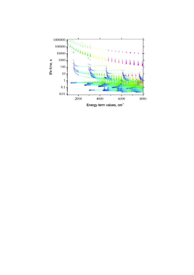
Figure 1: Lifetimes of CH₄ computed using the 10to10 line list (Yurchenko & Tennyson, 2014). The colors range from dark blue ($J=0$) to red ($J=45$). See Tennyson et al. (2016a) for a full discussion of methane lifetimes.

2.3 Cooling function

The emissivity (erg$/$s sr molecule) can be used to produce the cooling function $W(T)$ as the total energy emitted by a molecule (Neale et al., 1996)

$$W(T)=\frac{1}{4\pi Q(T)}\sum_{\rm f,i}A_{\rm fi}\,hc\,\tilde{\nu}_{\rm fi}g_{\rm i}\exp\left(\frac{-c_{2}\tilde{E}_{\rm i}}{T}\right).$$ (5)

2.4 Stick spectra

A stick spectrum is a list of frequencies and line intensities, accompanied by the full description (quantum numbers) of the upper and lower states. When plotted, each line is represented by a ‘stick’ with the intensity given by its height, see Table 1 where an extract from an output file containing an absorption stick spectrum of KCl (Barton et al., 2014) is shown. A stick spectra of CaO is shown in Fig. 2.

Table 1: Extract from a stick spectrum output generated using the KCl line list of Barton et al. (2014).

$\tilde{\nu}_{\rm fi}$	$I_{\rm fi}$ (cm/molecule)	$J^{\prime}$	$\tilde{E}^{\prime}$		$J^{\prime\prime}$	$\tilde{E}^{\prime\prime}$	$\varv^{\prime}$		$\varv^{\prime\prime}$
2.50210000E-01	3.27956194E-26	1	1096.1338	<-	0	1095.8836	4	<-	4
2.51764000E-01	1.20091306E-25	1	825.6787	<-	0	825.4269	3	<-	3
2.53325000E-01	4.44675257E-25	1	552.8938	<-	0	552.6404	2	<-	2
2.54891000E-01	1.66533127E-24	1	277.7596	<-	0	277.5047	1	<-	1
2.56466000E-01	6.30771280E-24	1	0.2565	<-	0	0.0000	0	<-	0
4.94245000E-01	2.01890019E-26	2	1630.6257	<-	1	1630.1315	6	<-	6
4.97324000E-01	7.23121652E-26	2	1364.7757	<-	1	1364.2784	5	<-	5
5.00417000E-01	2.61886416E-25	2	1096.6342	<-	1	1096.1338	4	<-	4
5.03524000E-01	9.58980316E-25	2	826.1822	<-	1	825.6787	3	<-	3
5.06644000E-01	3.55093592E-24	2	553.4004	<-	1	552.8938	2	<-	2
5.09779000E-01	1.32976733E-23	2	278.2693	<-	1	277.7596	1	<-	1
5.12927000E-01	5.03675191E-23	2	0.7694	<-	1	0.2565	0	<-	0

Figure 2: Stick spectra (cm/molecule) of CaO (Yurchenko et al., 2016a) compared the CDMS (Müller et al., 2005) rotational band at $T$=298 K.

2.5 Cross sections

A cross section $\sigma_{\rm fi}(\tilde{\nu})$ from a single line $f\leftarrow i$ is related to the corresponding integrated absorption coefficient $I_{\rm fi}$ as

$$I_{\rm fi}=\int_{-\infty}^{\infty}\sigma_{\rm fi}(\tilde{\nu})\;{\rm d\,}\nu,$$ (6)

where $\tilde{\nu}$ is a transitional wavenumber. By introducing a line profile $f_{\tilde{\nu}_{\rm fi}}(\tilde{\nu})$ the cross section (cm$/($molecule cm${}^{-1})$) can be defined as

$$\sigma_{\rm fi}(\tilde{\nu})=I_{\rm fi}f_{\tilde{\nu}_{\rm fi}}(\tilde{\nu}),$$ (7)

where $f_{\tilde{\nu}_{\rm fi}}(\tilde{\nu})$ is an integrable function with the area normalized to unity:

$$\int_{-\infty}^{\infty}f_{\tilde{\nu}_{\rm fi}}(\tilde{\nu})\;{\rm d\,}\tilde{\nu}=1.$$ (8)

Figure 3 shows an example of cross sections of H₂S at $T=300$ K and $2000$ K using the ExoMol line list of Azzam et al. (2016).

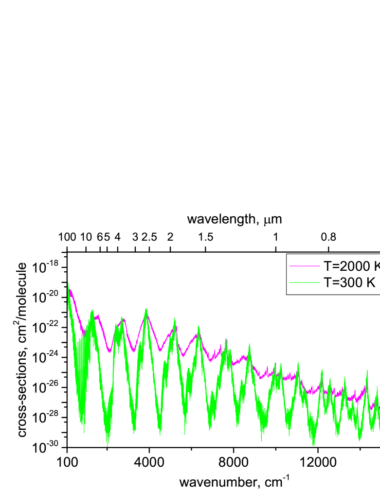
Figure 3: Absorption spectrum of H₂S at $T$ =300 K and 2000 K simulated using the ExoMol line list AYT2 (Azzam et al., 2016).

2.6 Grids

By default ExoCross uses an equidistant grid, defined by the wavenumber of wavelength range $[\tilde{\nu}_{A},\tilde{\nu}_{B}]$ and the number of the grid points $N_{\rm points}$. The latter includes both the first and last bounds. The grid bin size is defined by

$$\Delta\tilde{\nu}=\frac{\tilde{\nu}_{B}-\tilde{\nu}_{A}}{(N_{\rm points}-1)}.$$ (9)

The number of intervals is then $N_{\rm points}-1$. Usually the number of points is an odd number in order to make $\Delta\tilde{\nu}$ a ‘round’ value.

Non-equidistant wavenumbers grids can be generated either as grids of constant resolving power $R=\tilde{\nu}/\Delta\tilde{\nu}$ or equidistant wavelength grids.

2.7 Partition function and specific heat

The partition function $Q(T)$ is given by Eq. (2). The evaluation of $Q(T)$ requires the energy term values $\tilde{E}_{i}$ and degeneracies $g_{\rm tot}$, which are usually included in molecular line lists. As part of the intensity calculations, the partition function must be either evaluated using these quantities, or directly provided as part of the input. These values can be, e.g., taken from the .pf files provided as part of the ExoMol database (Tennyson et al., 2016b) or as part of the TIPS program provided by HITRAN (Gamache et al., 2017). The direct input option is recommended as often the ExoMol or HITRAN partition functions are more accurate as they contain additional, higher energy contributions which make an important contribution, particularly at elevated temperatures.

The molar specific heat is given by ($JK^{-1}$ mol^-1)

$$C_{p}(T)=R\left[\frac{Q^{\prime\prime}}{Q}-\left(\frac{Q^{\prime}}{Q}\right)\right],$$ (10)

where $R$ is the gas constant and the 1st and 2nd moments $Q^{\prime}$ and $Q^{\prime\prime}$ are

$$Q^{\prime} = T\frac{dQ}{dT},$$

$$Q^{\prime\prime} = T^{2}\frac{d^{2}Q}{dT^{2}}.$$

These latter moments can be also requested from ExoCross. An example of $C_{p}(T)$ of CH₄ generated using the 10to10 line list is shown in Fig. 4.

Figure 4: Specific heat $C_{p}(T)$ of CH₄ computed using the 10to10 line list Yurchenko & Tennyson (2014).

It is often instructive to plot individual contributions to the partition function from different $J$ states defined as

$$Q_{J}(T)=\sum_{n(J)}g_{n}^{\rm ns}(2J_{n}+1)e^{-c_{2}\tilde{E}_{n}^{J}/T}.$$ (11)

This is useful to assess the convergence of the line list with respect to $J$ and thus to estimate $T_{\rm max}$ the line list is applicable to. Figure 5 shows the such individual $Q_{J}(T)$ contributions for the UYT2 line list for SO₃ (Underwood et al., 2016a).

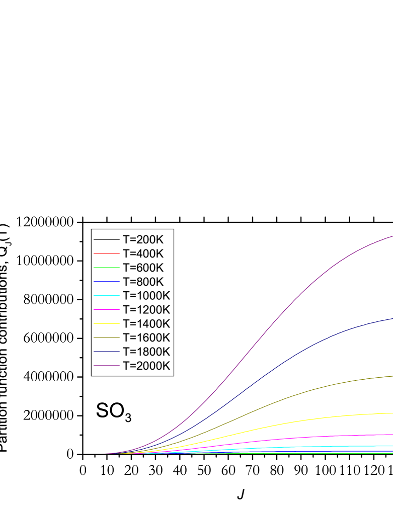
Figure 5: Contributions $Q_{J}(T)$ to the partition function of SO₃ using the line list UYT2 of Underwood et al. (2016a).

2.8 Intensity thresholds

An intensity threshold can be used to speed up the cross-section calculation or to reduce the output in stick-spectra type calculations (done by simply specifying a constant intensity threshold value in cm$/$molecule in the input file). The constant intensity cut-offs are however known to cause problems at long wavelengths, where the density of lines is small and each line, even weak, can be important. A more sophisticated method is to use the dynamic HITRAN’s intensity cut-off (Rothman et al., 2013), defined as

$$I_{\rm cut-off}=\left\{\begin{array}[]{cc}I_{\rm crit}\,(\tilde{\nu}/\!\tilde{\nu}_{\rm crit})\,\tanh\left({c_{2}\tilde{\nu}}/\!{\,2T}\right)&{\rm for}\ \tilde{\nu}\leq\tilde{\nu}_{\rm crit},\\ I_{\rm crit}&\tilde{\nu}>\tilde{\nu}_{\rm crit},\end{array}\right.$$

where the HITRAN values for $\tilde{\nu}_{\rm crit}$ and $I_{\rm crit}$ are 2000 cm^-1 and $10^{-29}$ cm$/$molecule, respectively. These values are also default in ExoCross  but can be changed in the input.

2.9 HITRAN

ExoCross can be used to work with the line list in the HITRAN native format .par, which covers almost all its functionality. It can also be used to convert to ExoMol to HITRAN format (see Section 5.2).

2.10 Phoenix

ExoCross has the facility to output data in Phoenix format (Jack et al., 2009). In order to speed up the line-by-line calculations Phoenix’s atomic and molecular line lists have a compact structure, where all required properties (line positions, oscillator strengths, lower state energies and broadening parameters) are stored as 4- and 2-bytes integers. For the wavelength ($\mu$m, 4 byte-integers) this is defined as:

$$i_{\lambda}={\rm int}\left(\frac{\log(\lambda)}{R_{\log}}+0.5\right),$$

where

$$R_{\log}=\log\left(1.0+\frac{1.0}{2000000.0}\right).$$

The oscillator strength $gf_{\rm fi}$ for a $f\leftarrow i$ transition, energy term values $\tilde{E}$, and broadening parameters $\gamma$ and $n$ are mapped onto 2-byte integers according to

$$i_{p}={\rm int}\left(\log(p)\frac{1.0}{0.001\,\log(10.0)}\right)+2^{14},$$

where $p$ is one of these properties. The integers $i_{\lambda}$, $i_{\gamma}$ and $i_{n}$ are then written as unformatted records with direct access, each of which containing data for 65536 lines (block-size). For molecules the broadening parameters include the reference Voigt line widths due to H₂ ($\gamma_{{\rm H}_{2}}$) and He ($\gamma_{\rm He}$) and the corresponding temperature exponents $n_{{\rm H}_{2}}$ and $n_{\rm He}$ (see below). It should be noted that Phoenix uses the so-called astrophysics-convention for the nuclear statistical weights, which are related to the physics convention (adopted by ExoMol and HITRAN) as follows:

$$g_{\rm i}^{\rm ns-astro}=\frac{g_{\rm i}^{\rm ns-phys}}{\sum_{i}g_{\rm i}^{\rm ns-phys}},$$ (12)

where $i$ counts different nuclear statistics. For example, in case of water (H₂¹⁶O), the nuclear statistics $g_{i}^{\rm ns}$ factors (physics convention) are 1 (para) and 3 (ortho), thus $g_{i}^{\rm ns}$ in the astrophysics convention are 1$/$4 (para) and 3$/$4 (ortho). Since Phoenix’s partition functions are directly affected by the astrophysics convention, in order to be consistent, the ExoMol $gf_{\rm fi}$ values have to be scaled by the factor $1/4$ for water, or $\left(\sum_{i}g_{\rm i}^{\rm ns-phys}\right)^{-1}$ in general.

2.11 Treating non-local thermodynamic equilibrium (non-LTE)

ExoCross provides a simple approach to treating non-LTE environments by differentiating between the rotational and vibrational (vibronic) temperatures when calculating intensities or partition functions (or other $T$-dependent properties). To this end we approximate the total energy as a sum of the vibrational (or vibronic) and rotational contributions;

$$\tilde{E}_{\varv,J,k}=\tilde{E}_{\varv}^{\rm vib}+\tilde{E}_{J,k}^{\varv,\rm rot},$$ (13)

where $\varv$ and $k$ are generic vibrational (vibronic) and rotational quantum numbers, respectively. If the pure vibronic contributions are taken as the corresponding energy values at $J=0$ (integer spin), $J=1/2$ (non-integer spin) or the lowest $J$ allowed by the symmetry of the electronic term and the parity, corresponding to the lowest states (usually ‘+’ or ‘e’). The rotational contribution is simply given by

$$\tilde{E}_{J,k}^{\varv,\rm rot}=\tilde{E}_{\varv,J,k}-\tilde{E}_{\varv}^{\rm vib}.$$ (14)

We also assume that the rotational and vibrational modes are in corresponding (Boltzmann) LTE and that the non-LTE population of a given state (used in intensity and/or partition function calculations) is given by

$$F_{J,\varv,k}(T_{\rm vib},T_{\rm rot})=e^{-c_{2}\tilde{E}_{\varv}^{\rm vib}/T_{\rm vib}}e^{-c_{2}\tilde{E}_{J,k}^{\varv,\rm rot}/T_{\rm rot}}.$$

For this representation it is important to have all the vibrational and rotational quantum numbers defined in the line list, or at least for states accessed by non-LTE calculations.

3 Line profiles

The line broadening is important for practical applications. While temperature effects are commonly modelled by a Doppler line profile, pressure broadening is more complicated. For very high pressure regimes Lorentzian profiles can be used, while for moderate pressures Voigt profiles are generally used (see, for example, Schreier (2017)).

3.1 Standard line profiles and sampling method

The most commonly used line profiles in ExoCross include Gaussian, Doppler, Voigt and Lorentzian.

The general Gaussian line profile is given by (Hill et al., 2013b)

$$f^{\rm G}_{\tilde{\nu}_{\rm fi},\alpha_{\rm G}}(\tilde{\nu})=\sqrt{\frac{\ln 2}{\pi}}\frac{1}{\alpha_{\rm G}}\exp\left(-\frac{(\tilde{\nu}-\tilde{\nu}_{\rm fi})^{2}\ln 2}{\alpha_{\rm G}^{2}}\right),$$ (15)

where $\tilde{\nu}_{\rm fi}$ is the line centre position and $\alpha_{\rm G}$ is the Gaussian half-width at half-maximum (HWHM). The Gaussian line profile is useful to model generic spectra represented by lines with constant HWHM. The Gaussian line profile can be also used to model the microturbulence broadening by choosing $\alpha_{\rm G}$ appropriately.

The Doppler line profile $f^{\rm D}_{\tilde{\nu}_{\rm fi},\alpha_{\rm D}}(\tilde{\nu})$ is based on the Gaussian shape defined in Eq. (15), where the Doppler HWHM is given by

$$\alpha_{\rm D}=\sqrt{\frac{2k_{\mathrm{B}}T\ln 2}{m}}\frac{\tilde{\nu}_{\rm fi}}{c},$$ (16)

at temperature $T$ for a molecule of mass $m$.

The Lorentzian profile is given by

$$f^{\rm L}_{\tilde{\nu}_{\rm fi},\gamma_{L}}(\tilde{\nu})=\frac{1}{\pi}\frac{\gamma_{L}}{(\tilde{\nu}-\tilde{\nu}_{\rm fi})^{2}+\gamma_{L}^{2}},$$ (17)

where $\gamma_{L}$ is the Lorentzian line width (HWHM), given most commonly by

$$\gamma_{L}=\gamma_{L}^{0}\left(\frac{T_{0}}{T}\right)^{n_{L}}\frac{P}{P_{0}}.$$ (18)

Here $T_{0}$ and $P_{0}$ are the reference temperature and pressure, respectively, $\gamma_{0}$ and $n_{L}$ are broadening parameters for a given broadener, reference HWHM and temperature exponent, respectively.

The Voigt profile is a convolution of the Doppler and Lorentazian profiles:

$$f^{\rm V}_{\tilde{\nu}_{\rm fi},\alpha_{\rm D},\gamma_{\rm L}}(\tilde{\nu})=\frac{\gamma_{\rm L}\ln 2}{\pi^{3/2}\alpha_{\rm D}}\int_{-\infty}^{\infty}\frac{e^{-y^{2}}{\rm d\,}y}{(\nu-y)^{2}+\gamma_{\rm L}^{2}},$$ (19)

where we introduced a unitless variable $\nu$ given by:

$$\nu=\frac{(\tilde{\nu}-\tilde{\nu}_{\rm fi})\ln 2}{\alpha_{D}}.$$ (20)

The Lorentzian line width $\gamma_{\rm L}$ strongly depends on the molecule and is usually also state-dependent. The corresponding values must be given in the input including the specification of the broadeners and their mixing ratio. Each calculation can handle only one combination of broadeners.

Additionally, a simple box-type line profile given by

$$f_{\Delta\tilde{\nu}}^{\rm B}(\tilde{\nu})=\left\{\begin{array}[]{cc}1/\Delta\tilde{\nu},&|\tilde{\nu}-\tilde{\nu}_{\rm fi}|\leq\Delta\tilde{\nu}\\ 0,&|\tilde{\nu}-\tilde{\nu}_{\rm fi}|>\Delta\tilde{\nu},\end{array}\right.$$ (21)

where $\Delta\tilde{\nu}$ is the width of the box, is available.

The individual contribution from each line to the cross sections at a given frequency grid point $k$ is evaluated by sampling the corresponding line profile (see Eq. 7) a given by

$$\sigma_{\rm fi}(\tilde{\nu}_{k})=I_{\rm fi}f_{\tilde{\nu}_{\rm fi}}(\tilde{\nu}_{k}),$$

which will be often referred to as a sampling method. This method has the disadvantage of underestimating the opacity when too coarse grids are used which can lead to lines being partially or completely left out. This is a typical problem for long wavelengths where the lines are narrow and far from each other, which is usually tackled either by re-normalizing the line area, see, for example, Sharp & Burrows (2007), or by using a random sampling (Lupu et al., 2016). Below we explore a different, more rigorous alternative.

In practical applications the cross sections are computed on a grid of frequencies (wavenumbers) $\tilde{\nu}_{i}$. When the grid is not sufficiently dense, the line profiles lose their normalisation. This is usually not a problem, at least for most of the room temperature applications. However for high $T$ when billions of lines are used, this leakage can lead to a significant loss of opacity. In order to prevent this effect, Hill et al. (2013b) suggested using an averaged intensity over a given frequency bin, where the corresponding cross section is integrated analytically. This method originally presented for the Gaussian (Doppler) line profile, is extended here to describing Lorentzian and Voigt profiles.

3.2 Binned Gaussian profile with analytical integrals

An averaged (integrated) cross section over a bin $[\tilde{\nu}_{k}-\Delta\tilde{\nu}/2\ldots\tilde{\nu}_{k}+\Delta\tilde{\nu}/2]$ from a line f$\leftarrow$ i is given by

$$\bar{\sigma}_{k}^{\rm fi} = \frac{I_{\rm fi}}{\Delta\tilde{\nu}}\int_{\tilde{\nu}_{k}-\Delta\tilde{\nu}/2}^{\tilde{\nu}_{k}+\Delta\tilde{\nu}/2}f^{\mathrm{G}}_{\tilde{\nu}_{\rm fi},\alpha_{\rm fi}}(\tilde{\nu})\,{\rm d\,}\tilde{\nu}$$ (22)

$$= \frac{I_{\rm fi}}{2\Delta\tilde{\nu}}\left[{\rm erf}(x_{k,\rm if}^{+})-{\rm erf}(x_{k,if}^{-})\right],$$ (23)

where erf is the error function and

$$x_{k,\rm fi}^{\pm}=\frac{\sqrt{\ln 2}}{\alpha_{\rm D}}\left[\tilde{\nu}_{k}\pm\frac{\Delta\tilde{\nu}}{2}-\tilde{\nu}_{\rm fi}\right]$$ (24)

are the scaled limits of the wavenumber bin centred on $\tilde{\nu}_{k}$ relative to the line centre, $\tilde{\nu}_{\rm fi}$, and $I_{\rm fi}$ is the line intensity in units of cm${}^{-1}/$molecule cm^-2 from Eq. (1). Here we take advantage of the fact that an analytical solution exists for the integral of the Gaussian function

$$\int e^{-x^{2}}{\rm d\,}x=\frac{\sqrt{\pi}}{2}{\rm erf(x)}+C,$$ (25)

where $C$ is an integration constant. The total cross section at the frequency bin $k$ is given by a sum over all contributions from individual lines $\rm fi$:

$$\bar{\sigma}_{k}=\sum_{\rm fi}\bar{\sigma}_{k}^{\rm fi}$$ (26)

and can be interpreted as an average value of the cross sections from a given frequency bin $k$. The advantage of this approach is that in definition it always gives exact integrated cross sections independent of the number of grid points used or the integration interval. Therefore it is recommended for applications where accurate integrated cross sections or absorption coefficients on coarse grids are required. However it is known that averaged cross sections, especially on coarse grids, can lead to huge errors in integrated flux. Therefore for radiative transfer applications, the direct sampling methods are more accurate and should be used instead.

3.3 Binned Lorentzian profile with analytical integrals

Here we apply the same idea of analytical integral to the Lorentzian line profile:

$$\bar{\sigma}_{k}^{\rm fi} = \frac{I_{\rm fi}}{\Delta\tilde{\nu}}\int_{\tilde{\nu}_{k}-\Delta\tilde{\nu}/2}^{\tilde{\nu}_{k}+\Delta\tilde{\nu}/2}f^{\mathrm{L}}_{\tilde{\nu}_{\rm fi},\alpha_{\rm fi}}(\tilde{\nu})\,{\rm d\,}\tilde{\nu}$$ (27)

$$= \frac{I_{\rm fi}}{\pi\Delta\tilde{\nu}}\left[\arctan(y_{k,\rm fi}^{+})-\arctan(y_{k,\rm fi}^{-})\right],$$ (28)

where

$$y_{k,\rm fi}^{\pm}=\frac{\tilde{\nu}_{k}\,\tilde{\nu}_{\rm fi}\,\pm\,\Delta\tilde{\nu}/\!2}{\gamma_{\rm L}}.$$ (29)

Here the following integral was used:

$$\int\frac{{\rm d\,}x}{x^{2}+\gamma^{2}}=\frac{1}{\gamma}\arctan\left(\frac{x}{\gamma}\right)+C,$$

where $C$ is an integration constant. Again, the integration within each bin is done analytically which guarantees no loss of accuracy for any number of points.

3.4 Binned Voigt profile with analytical integrals

The two line profiles (Gaussian and Loretnzian) can be combined to produce a similar formulation for the Voigt profile, where we use the idea of Gauss-Hermit quadratures as, for example, used in Humlíček’s algorithm (Humlicek, 1979). The Voigt convolution integral in Eq. (19) can be written using these quadratures as follows:

$$f^{\rm V}_{\tilde{\nu}_{\rm fi},\alpha_{D},\gamma_{L}}(\tilde{\nu})=\frac{\gamma_{\rm L}\ln 2}{\pi^{3/2}\alpha_{\rm D}^{2}}\sum_{k=1}^{N_{\rm G-H}}\frac{w_{k}^{\rm G-H}}{(\nu-\nu_{k})^{2}+\gamma_{\rm L}^{2}}.$$ (30)

where $\nu_{k}$ and $w_{k}^{\rm G-H}$ are the Gauss-Hermite quadrature points and weights, respectively ($k=1\ldots N_{\rm G-H}$) and $\nu$ is related to $\tilde{\nu}$ via Eq. (20). In this form the computation of Voigt can be also generalised to produce the area-conserved integrals using Eq. (28):

$$\sigma_{ij}^{\rm V}=\frac{I_{\rm fi}}{\pi^{3/2}\Delta\tilde{\nu}}\ \sum_{k=1}^{N_{\rm G-H}}w_{k}^{\rm G-H}\left[\arctan(y_{k,\rm fi}^{+})-\arctan(y_{k,\rm fi}^{-})\right].$$ (31)

where $y_{k,\rm fi}^{\pm}$ is defined in Eq. (29). We usually take $N_{\rm G-H}=30$ Gauss-Hermite points. This approach does not appear to have been taken previously.

3.5 Vectorized Voigt approximation

Evaluation of Voigt line profile is generally one of the biggest bottlenecks in opacity calculations. Here we present a new approximate cross section algorithm for the Voigt line profile, which leads to efficient vectorization and thus fast calculations. Our approach is based on the observation that the shape of the wings of the Voigt profile ($>4$ cm^-1 from the line centre), at least for Humlíček’s algorithm, is relatively constant over the large variation of $\tilde{\nu}$ as Lorentzian broadening is generally the largest contributor. For example, Figure 6 shows how the wings of the Voigt profile centred at $\tilde{\nu}_{\rm fi}=1$ differ from the wings of other Voigt profiles centred at all other $\tilde{\nu}_{\rm fi}$ across the entire wavenuber range from 0 to 30 000 cm^-1 (computed using Humlíček’s algorithm). As expected, the error grows as the Doppler HWHM (Eq. 16) increases with transition wavenumber. However this never exceeds more than 1% for even the lowest pressure. One of the most interesting observations is that at $10^{0}$ bar, the relative error is almost the same as the mostly Doppler profile error at 10^-20 bar. With higher pressures this error falls significantly to lower than 10^-2 % and lower temperatures reduces this by orders of magnitudes. It is only around the line centre, which we estimate to be within 4 cm^-1, that the variation of the line shape of the Voigt profile is important.

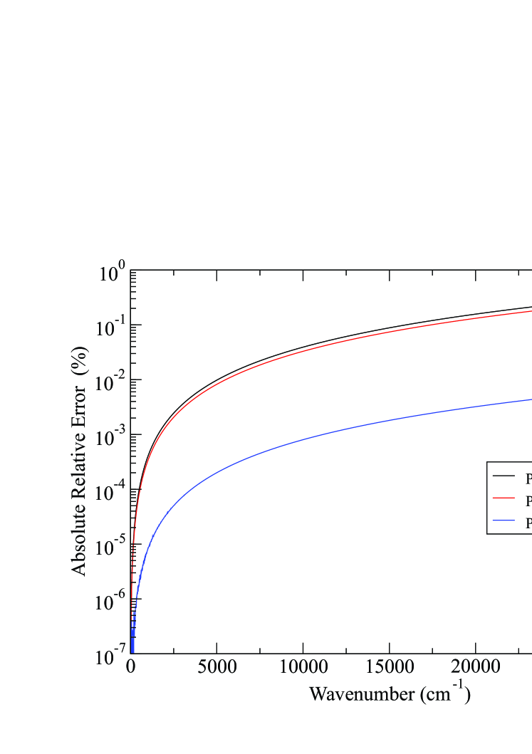
Figure 6: Plot of absolute relative error at 4 cm^-1 for the Voigt profile at $\tilde{\nu}$ against $\tilde{\nu}=1.0$ cm^-1 for H₂O with T=5000 K and $\gamma_{L}$ computed from Eq. (18) with parameters $\gamma_{L}^{0}=0.0709$, $T_{0}=296.0$ K, $n_{L}=0.5$, $P_{0}=1$ and pressure $P$ at 10^-20, 10⁰ and 10¹ bar.

Based on this observation, the Voigt profile $f^{\rm V-V}_{\tilde{\nu}_{\rm fi},\alpha_{\rm D},\gamma_{\rm L}}(\tilde{\nu})$ can be split into two parts as follows (omitting the indeces $\alpha_{\rm D},\gamma_{\rm L}$ for simplicity):

$$f^{\rm V-V}_{\tilde{\nu}_{\rm fi}}(\tilde{\nu})=\begin{cases}f^{\rm V}_{\tilde{\nu}_{\rm fi}}(\tilde{\nu}),&|\tilde{\nu}-\tilde{\nu}_{\rm fi}|\leq 4\;{\rm cm}^{-1}\\ f_{\alpha_{\rm D},\gamma_{\rm L}}^{\text{ref}}(\tilde{\nu})\,\beta_{\tilde{\nu}_{\rm fi}},&|\tilde{\nu}-\tilde{\nu}_{\rm fi}|>4\ {\rm cm}^{-1}\end{cases}$$ (32)

where ${f_{\alpha_{\rm D},\gamma_{\rm L}}^{\text{ref}}}(\tilde{\nu})$ is a reference Voigt profile centred at $\tilde{\nu}_{\rm fi}=1$ cm^-1:

$$f_{\alpha_{\rm D},\gamma_{\rm L}}^{\text{ref}}(\tilde{\nu})=f^{\rm V}_{1\,{\rm cm}^{-1}}(\tilde{\nu}).$$

Here $\beta_{\tilde{\nu}}$ is a parameter that is used to prevent discontinuities at $\tilde{\nu}=\tilde{\nu}_{\rm fi}\pm 4$ cm^-1  when switching between the two profiles and is given by:

$$\beta_{\tilde{\nu}_{\rm fi}}=\frac{f^{\rm V}_{\tilde{\nu}_{\rm fi}}(4\,{\rm cm}^{-1})}{f_{\alpha_{\rm D},\gamma_{\rm L}}^{\text{ref}}(4\,{\rm cm}^{-1})}.$$ (33)

This parameter is included for completeness and is generally set to $\beta=1$ for a performance boost as the discontinuities are not visible at most scales for a single transition and invisible once the whole spectrum is considered. For a given set of pressure broadening parameters $\gamma_{\rm L}$ we pre-compute a set of points defining the wings $f_{\alpha_{\rm D},\gamma_{\rm L}}^{\text{ref}}$ and then simply select a relevant set. Therefore the only palce where real Voigt calculation needs to be done is around the centre. Additionally, (if used) $\beta_{\tilde{\nu}_{\rm fi}}$ needs to be calculated at the boundary, which completes the evaluation of the given profile.

The algorithm is based on the (Humlicek, 1979) approximation for the Voigt profile in Eq. (19), which is the main method used by ExoCross. The Humlíček algorithm is called only for the regions within 4 cm^-1 from the line centre. Using the conventionally used Lorentz cutoff of 25 cm^-1, this means that only up to 8% of the calculation is computationally demanding giving a theoretical speed up of 12.5 times. This is illustrated in Figure 7, which shows speed up using our Vectorized Voigt algorithm when applied to the region of 0.0–300 cm^-1  of the BT2 water linelist (Barber et al., 2006) at T=1900 K and P=1 bar. The speed up $S$ for $N$ points used to bin the wavenumber grid is defined as:

$$S^{N}=\frac{T^{N}_{0}}{T^{N}_{\rm V-V}},$$ (34)

where $T^{N}_{0}$ is the time required for a standard Humlíček computation on a wavenumber grid $N$ and $T^{N}_{\rm V-V}$ is the time required using the Vectorized Voigt method. The speed up converges to a maximum value of about 11 times compared to the standard Humlíček calculation, close to the predicted maximum speed up.

This procedure is also efficiently vectorized. Firstly, for the inner part (top of Eq. (32)), which is symmetric, only one half is computed. The other half is then merely looped through backwards and applied to the grid, requiring only to multiply by the absorption coefficient (emissivity) and to add to the opacity grid. The second vectorization occurs when dealing with the second part of Eq. (32). Here again, only a multiplication by the intensity and add to the opacity grid is required. These two loops are vectorized through the Fused-Multiply-Add (FMA) instruction.

Figure 8 presents an illustration, where both the Vectorized and standard (Humlíček) Voigt methods were used to generate cross sections of water from the BT2 line list for T=1900 K and P=1 bar. The new algorithm captures all features with the total opacity for the range shown differing by only by 10^-6 cm² molecule^-1.

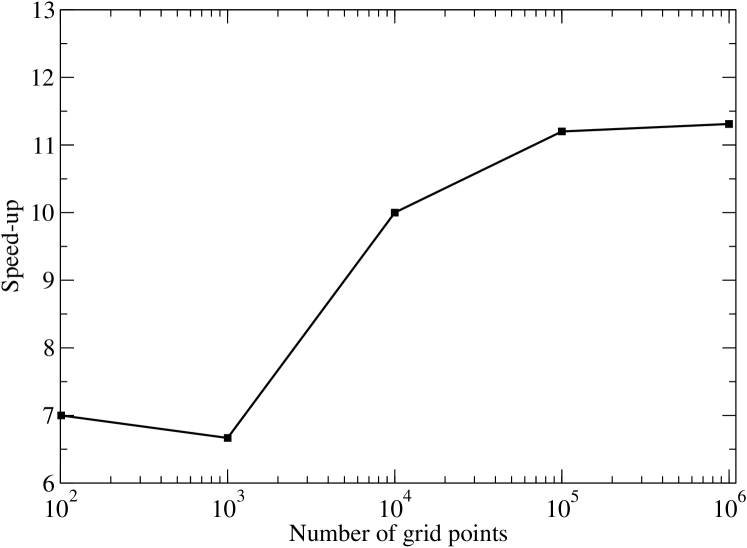
Figure 7: Speed up, Eq. (34), for the Vectorized Voigt method against the standard Voigt (Humlíček) computed on varying wavenumber grid sizes ($N$) using the BT2 (Barber et al., 2006) water line list computed at T=1900 K, P=1 bar and wavenumber range between 0 cm^-1 and 300 cm^-1 

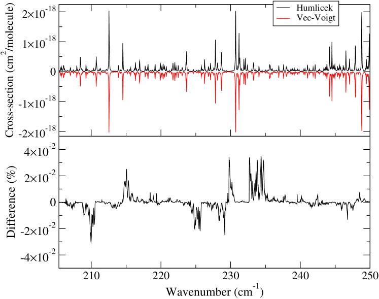
Figure 8: Top plot: Comparison of cross section calculations for the BT2 water line list (Barber et al., 2006) between the standard Humlíček and the Vectorized Voigt method with $T=$1900 K. Bottom plot: Percentage difference between the Humlíček and Vectorized Voigt method. The calculations used no intensity threshold and a wavenumber bin of 0.1 cm^-1.

Lastly, for a full opacity calculation between 0.0–30 000 cm^-1, Table 2 shows that using no intensity threshold with the Vectorized Voigt method is almost 3.5 times faster than the full Humlíček method at 10^-30 cm molecule^-1 thresholding. Comparing like for like, the Vectorized Voigt is around 10 to 12 times faster compared to the standard Humlíček method.

Table 2: Time taken (s) for differing methods and intensity thresholds (cm molecule^-1) to compute opacities using the 500 million transitions of the BT2 water line list (Barber et al., 2006) between 0 and 30 000 cm^-1 with a wavenumber binning of 0.1 cm^-1. I/O time is not considered. Test was performed on single core on an Intel Core i5-2500 CPU at 3.30GHz with 16 GB RAM

Method	Threshold	Time(s)
Vec-Voigt	0	251.2
Humlíček	0	2775.6
Vec-Voigt	10-30	70.0
Humlíček	10-30	832.6

Future development of the algorithm will look into automatically tuning the distance from the line centre depending on the temperature and pressure parameters given.

3.6 Binned Vectorized Voigt with the line area preserved

Considering the importance of preserving integrated cross section in many applications, we also provide an alternative version of the Vectorized Voigt, based on re-normalization of the line area. During the precomputation stage of the Vectorized Voigt method, the total sum for all points ($\Sigma_{\alpha_{\rm D},\gamma_{\rm L}}$) that lie above $|\tilde{\nu}-\tilde{\nu}_{\rm fi}|>4$ cm^-1 is computed and stored alongside the reference Voigt profile. When computing the Vectorized Voigt on a transition, the central Humlíček region is evaluated into a temporary array and its sum is added to $\Sigma_{\alpha_{\rm D},\gamma_{\rm L}}$. After which the scaled absolute intensity $\tilde{I}_{fi}$ is computed as:

$$\tilde{I}_{fi}=\frac{I_{fi}}{\Sigma_{\alpha_{\rm D},\gamma_{\rm L}}}$$ (35)

Both the temporary Humlíček array and reference Voigt is applied to the opacity grid with the scaled intensity $\tilde{I}_{fi}$.

Table 3: Table showing percentage relative error between the total summed absolute intensity and the total integrated intensity for BT2 water line list computed between 0 and 300 cm^-1 at $T$=1900 K and $P$=1 bar at various wavenumber binnings. The total integrated intensities are computed using Humlíček (H), Vectorized Voigt (VV) and the Normalized Vectorized Voigt (VVN).

		Error
Bin (cm-1)	H(%)	VV (%)	VVN (%)
10.00	41.62	41.63	0.01
1.00	37.59	37.59	0.73
0.10	1.66	1.66	0.17
0.01	0.07	0.07	0.01

Whilst not a proper treatment of area conservation as that given by Eq. (31), it serves as a reasonable approximation and, as shown in Table 3, gives good results within 1% of the total summed absolute intensity for even large wavenumber bins. To our knowledge, this method does not appear to be reported before.

3.7 Broadening parameters

The Voigt profile as a convolution of Doppler and Lorentzian profiles requires definition of the corresponding line widths (HWHM), $\alpha_{\rm D}$ (see Eq. (16)) and $\gamma_{\rm L}$, given by Eq. (18). The Doppler parameter $\alpha_{\rm D}(T)$ is easy to deal with. It does not depend on the molecular states, only the line position and can be always computed on the fly. The Lorentzian (Voigt) parameters $\gamma_{0}(P_{0},T_{0})$ and $n_{L}$ however are very different for different molecules. Besides they show a pronounced dependence on the state quantum numbers, with the rotational ($J$) state dependence being the strongest.

The two-file format of the ExoMol database requires special structure for the broadening parameters. Instead of using the conventional line-by-line approach employed by spectroscopic databases such in HITRAN (Gordon et al., 2017) or GEISA (Jacquinet-Husson et al., 2016), where the pressure broadening is specified for the each transitions, ExoMol’s broadening parameters are stored in separate files with the extension .broad (Tennyson et al., 2016b). This structure is justified for most applications as the same parameters are usually used for a large number of different transitions. The latter is either due to the absence of broadening information on all the lines or due to the weak dependence of these parameters for different states. This structure was recently implemented for a number of molecules including H₂O, CH₄ and HCN (Barton et al., 2017; Yurchenko et al., 2017b). Table 4 shows an extract from the .broad file for CS as an example. Each line in .broad has the following structure: type (a0, a1, $\ldots$), $\gamma_{0}(P_{0},T_{0})$, $n_{L}$ and quantum numbers defined by the type.

Currently ExoCross supports three following broadening schemes, constant, a0 and a1, depending on the rigorous quantum numbers $J^{\prime}$ and $J^{\prime\prime}$. The simplest case is when $\gamma_{0}(P_{0},T_{0})$ and $n_{L}$ are constant and the .broad data is not required. The a0 type corresponds to the $J$-dependence only. In this case the 4th column in the .broad file contains the $J$ values. The $J$ quantum number is a mandatory quantity in the ExoMol format (column 4 in .states) and is therefore relatively straightforward to handle. A similar scenario (a1) is when the broadening depends on the upper $J^{\prime}$ (column 5 in .broad) and lower $J^{\prime\prime}$ (column 4) rotational quantum numbers. All other broadening schemes involve dependence on some non-rigorous quantum numbers (‘labels’), such as vibrational $\varv$ or rotational $K$. The non-rigorous quantum numbers and their position in the .states file are molecule dependent and thus need to be specified. This information can be found in the ExoMol’s .def (API) file. The current version of ExoCross supports rigorous quantum numbers only and therefore does not require interfacing with the ExoMol database.

Table 4: Air .broad file for ¹²C³²S: portion of the file (upper part); field specification (lower part).

a0	0.0860	0.096	0
a0	0.0850	0.093	1
a0	0.0840	0.091	2
a0	0.0840	0.089	3
a0	0.0830	0.087	4
…
a0	0.0720	0.067	35
a0	0.0720	0.066	36
…

Field	Fortran Format	C format	Description
code	A2	$\%$2s	Code identifying quantum number set following $J^{\prime\prime}$*
$\gamma_{0}(P_{0},T_{0})$	F6.4	%6.4f	Lorentzian half-width at reference temperature and pressure in cm-1/bar
$n_{L}$	F5.3	%5.3f	Temperature exponent
$J^{\prime\prime}$	I7/F7.1	$\%$7d	Lower $J$-quantum number

*Code definition: a0 = none

3.8 Mixtures of broadeners

We consider different broadeners to be independent and their effect additive. Thus the total value of $\gamma_{\rm L}$ is a weighed sum of $\gamma_{i}^{\rm L}$ from each broadener as given by:

$$\gamma_{\rm L}=\sum_{i}\gamma_{i}^{\rm L}\rho_{i}$$

where $\rho_{i}$ is the fraction portion of the $i$th broadener. Here we used the fact that the cross sections from each lines are additive and thus the line profile can be represented as a weighted average of lines broadened by different species.

3.9 Off-set

Even though, at least in principle, a line profile has infinite spread, in practical calculations a frequency (or wavelength) cut-offs must be applied to limit the calculation region to around the line centre only. Not only does this influence the computation time and the accuracy of cross sections, but it is also assumed in some applications as a point of convention. For example, water cross section are conventionally taken to have a 25 cm^-1 cutoff, with far-wing contributions outside this region assumed to form part of the so-called water-continuum (Shine et al., 2012). 25 cm^-1 is the default cut-off value in ExoCross, alternatively it is specified in the input file.

3.10 Super-lines

The super-line approach is an efficient method for describing a molecular broadened continuum originally proposed by Rey et al. (2016) and was recently studied in detail by Yurchenko et al. (2017a). The super-lines are constructed as temperature-dependent intensity histograms as follows (see also detailed discussion by Rey et al. (2016)). We divide the wavenumber range $[\tilde{\nu}_{A},\tilde{\nu}_{B}]$ into $N$ frequency bins, each centred around a grid point $\tilde{\nu}_{k}$. For each $\tilde{\nu}_{k}$ the total absorption intensity ${I}_{k}(T)$ is computed as a sum of absorption line intensities $I_{\rm fi}$, as in Eq. (1), from all f $\to$ i transitions falling into the wavenumber bin $[\tilde{\nu}_{k}-\Delta\tilde{\nu}_{k}/2\ldots\tilde{\nu}_{k}+\Delta\tilde{\nu}_{k}/2]$ at the given temperature $T$. Each grid point $\tilde{\nu}_{k}$ forms a super-line of an artificial transition with an effective absorption intensity ${I}_{k}(T)$. The super-line lists are given in a two-column format $\{\tilde{\nu}_{k},{I}_{k}(T)\}$ with pre-computed intensities ${I}_{k}$, in the same format as used to store ExoMol cross-sections (Tennyson et al., 2016b). The filename have the extension .super. The super-lines approach does not require that histograms are of the same widths $\Delta\tilde{\nu}_{k}$ and can accept non-equidistant grids as well, see below.

The histograms in ExoCross can be produced as cross sections using the Bin-option in the input file (see Manual), which is basically just a sum of all intensities within a given bin $i$. Ones the histograms are computed (in the standard cross section two-column format), they can be treated as normal line lists. In this case the .states file is not needed as all the information has been already included into the line position and intensity. Moreover, since the states-specific information is completely lost from the line characteristics, the state-dependent line profiles can not be used for temperature/pressure broadening. Doppler line profiles require no information on the upper/lower states and are not restricted. However for the Voigt pressure broadening parameters, which usually depend (at least) on $J$, only constant values of $\gamma_{0}$ and $n_{L}$ (see Eq. (18)) can be used in conjunction with super-lines. For this reason the super-lines are recommended for description of featureless continuum produced from the weaker lines only. The stronger lines should be treated as usual, line-by-line.

3.11 User-defined profiles

New line profiles, see Tennyson et al. (2014) for example, can be easily implemented to ExoCross by the user. A detailed description is provided in the manual. The HITRAN option in ExoCross can be used as an example.

4 Calculation protocol

The typical ExoCross calculation includes the following steps (see Fig. 9):

1. Read input instruction;

2. Read the .states file: energies, quantum numbers and statistical weighs;

3. Compute the partition function (if required);

4. Read $N$ lines with upper/lower IDs and the Einstein coefficient lines from the .trans file;

5. Apply filters;

6. Compute line intensities (absorption coefficients or emissivities, if required).

7. Compute cross sections on a grid of wavenumbers (if required);

8. Compute lifetimes (if required);

9. Compute cooling functions (if required);

10. Print the cross sections (stick spectra, life times, cooling functions) into a separate file;

11. Do time and memory reporting.

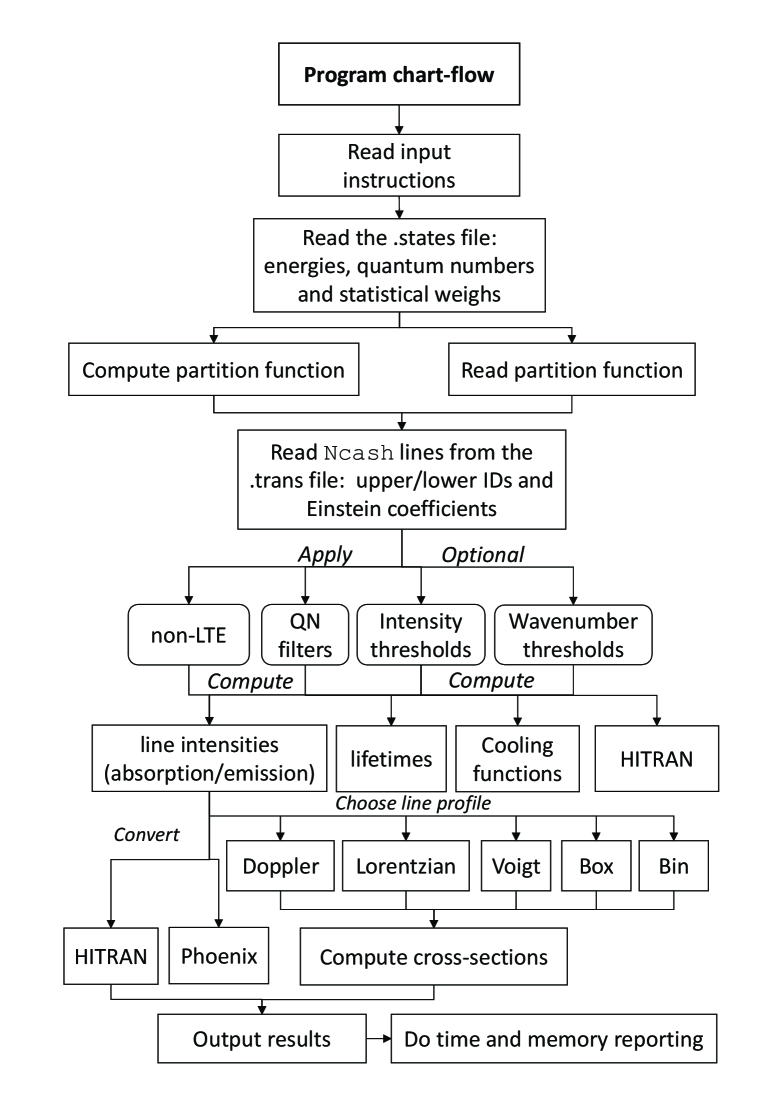
Figure 9: ExoCross program work-flow.

5 Data formats

ExoCross currently takes in input in either ExoMol or HITRAN format. It can provide output in these formats and in the format used by the Phoenix radiative transport code (Jack et al., 2009). These formats are discussed in turn below.

5.1 ExoMol format

A line list is defined as a catalogue of transition frequencies and intensities (Tennyson & Yurchenko, 2012). In the basic ExoMol format (Hill et al., 2013b), adopted by ExoCross, a line list has a compact structure consisting of two files: ‘States’ and ‘Transitions’; an example for the list NOname line list for ¹⁴N¹⁶O (Wong et al., 2017) is given in Tables 5 and 6. The ‘States’ (.states) file contains energy term values supplemented by the running number $n$, total degeneracy $g_{n}^{\rm tot}$, rotational quantum number $J_{n}$ (all obligatory fields), other quantum numbers and labels (both rigorous and not rigorous), lifetimes and Landé $g$-factors. For example for a generic open-shell diatomic molecule, the quantum numbers include $\upsilon$, $\Lambda$, parity ($\pm$), $\Sigma$, $\Omega$ and the electronic state label (e.g. X2Sigma+) (Yurchenko et al., 2016b). The ‘Transitions’ (.trans) file contains three obligatory columns, the upper and lower state indexes $n_{f}$ and $n_{i}$ which are running numbers from the ‘State’ file, and the Einstein coefficient $A_{\rm fi}$. For the convenience it also sometimes provides the wavenumbers $\tilde{\nu}_{fi}$ as the column 4. The line list in the ExoMol format can be used to simulate absorption or emission spectra for any temperature in a general way.

Table 5: Extract from the states file of the ¹⁴N¹⁶O line list.

$n$	Energy (cm-1)	$g_{n}$	$J_{n}$	$\tau$	$g_{J}$	+/-	e/f	State	$\varv$	${\Lambda}$	${\Sigma}$	${\Omega}$
1	0.000000	6	0.5	inf	-0.000767	+	e	X1/2	0	1	-0.5	0.5
2	1876.076228	6	0.5	8.31E-02	-0.000767	+	e	X1/2	1	1	-0.5	0.5
3	3724.066346	6	0.5	4.25E-02	-0.000767	+	e	X1/2	2	1	-0.5	0.5
4	5544.020643	6	0.5	2.89E-02	-0.000767	+	e	X1/2	3	1	-0.5	0.5
5	7335.982597	6	0.5	2.22E-02	-0.000767	+	e	X1/2	4	1	-0.5	0.5
6	9099.987046	6	0.5	1.81E-02	-0.000767	+	e	X1/2	5	1	-0.5	0.5
7	10836.058173	6	0.5	1.54E-02	-0.000767	+	e	X1/2	6	1	-0.5	0.5
8	12544.207270	6	0.5	1.35E-02	-0.000767	+	e	X1/2	7	1	-0.5	0.5
9	14224.430238	6	0.5	1.21E-02	-0.000767	+	e	X1/2	8	1	-0.5	0.5
10	15876.704811	6	0.5	1.10E-02	-0.000767	+	e	X1/2	9	1	-0.5	0.5
11	17500.987446	6	0.5	1.01E-02	-0.000767	+	e	X1/2	10	1	-0.5	0.5
12	19097.209871	6	0.5	9.41E-03	-0.000767	+	e	X1/2	11	1	-0.5	0.5
13	20665.275246	6	0.5	8.83E-03	-0.000767	+	e	X1/2	12	1	-0.5	0.5
14	22205.053904	6	0.5	8.35E-03	-0.000767	+	e	X1/2	13	1	-0.5	0.5
15	23716.378643	6	0.5	7.94E-03	-0.000767	+	e	X1/2	14	1	-0.5	0.5
16	25199.039545	6	0.5	7.59E-03	-0.000767	+	e	X1/2	15	1	-0.5	0.5

$n$: State counting number.

$\tilde{E}$: State energy in cm^-1.

$g_{n}$: Total statistical weight, equal to ${g_{\rm ns}(2J_{n}+1)}$.

$J_{n}$: Total angular momentum.

$\tau$: Lifetimes (s^-1).

$g_{J}$: Landé $g$-factor

$+/-$: Total parity.

$e/f$: Rotationless parity.

State: Electronic state.

$\varv$: State vibrational quantum number.

$\Lambda$: Projection of the electronic angular momentum.

$\Sigma$: Projection of the electronic spin.

$\Omega$: $\Omega=\Lambda+\Sigma$, projection of the total angular momentum.

Table 6: Extract from the transitions file of the ¹⁴N¹⁶O line list.

$f$	$i$	$A_{\rm fi}$ (s-1)	$\tilde{\nu}_{\rm fi}$ (cm-1)
14123	13911	1.5571E-02	10159.167959
13337	13249	5.9470E-06	10159.170833
1483	1366	3.7119E-03	10159.177466
9072	8970	1.1716E-04	10159.177993
1380	1469	3.7119E-03	10159.178293
14057	13977	1.5571E-02	10159.179386
10432	10498	4.5779E-07	10159.187818
12465	12523	5.4828E-03	10159.216008
20269	20286	1.2448E-10	10159.227463
12393	12595	5.4828E-03	10159.231009
2033	2111	6.4408E-04	10159.266541
17073	17216	4.0630E-03	10159.283484
5808	6085	3.0844E-02	10159.298459
5905	5988	3.0844E-02	10159.302195
13926	13845	1.5597E-02	10159.312986

$f$: Upper state counting number;
$i$: Lower state counting number;
$A_{\rm fi}$: Einstein-A coefficient in s^-1;
$\tilde{\nu}_{\rm fi}$: transition wavenumber in cm^-1.

5.2 HITRAN

The current “HITRAN format” is fully specified in Table 1 of the 2004 edition of HITRAN (Rothman et al., 2005). This format, which is also used for the current release of the related high-temperature database HITEMP (Rothman et al., 2010), has been implemented here.

Although the HITRAN format is widely adopted as a de facto standard, we advise some caution before adopting it. The format is rather verbose and can become extremely unwieldy as a means of representing large line lists. The format is highly tuned towards Earth atmosphere application (e.g. in its choice pressure broadening parameters and temperature ranges) and is therefore rather inflexible for other applications. HITRAN themselves have recognised these issues and have introduced their own web-based interface HAPI Kochanov et al. (2016) to act as front end and to perform data compression. The database itself has moved to an online-version which provides much more flexibility than the 2004 format Hill et al. (2013a).

5.3 Improving data processing

Both the cross-section and intensity steps (see Fig. 9) are OpenMP parallelized. Users can specify the number of processors requested, which is otherwise set to 1 (no parallelization). In order to make reading and processing data from the .trans file more efficient, ExoCross reads line transitions in chunks of $N$ lines, not line-by-line. ‘Caching’ these records into RAM allows for the parallelization for both the transition filtering and of the computation of line-profiles. Each thread is given their own version of the opacity grid to perform work independently without the usage of atomic operations or mutex locks. The total opacity grid can be retrieved at the end of the program run combining all threads’ opacity arrays. This number $N$ is either specified in the input file or estimated based on the memory available on the system (default). The number of processors must be specified in the input as well (see below on the memory handling).

5.4 Filters

ExoCross allows the selection of specific bands/states when computing intensities using the ‘filter’ option. The filters are based on the column-numbers containing the corresponding quantum labels of the upper and lower states. For example, the vibrational quantum number $\varv$ in the NOname line list is given in the column number 10 (see Table 5), which can be used to generate absorption cross section of NO for the overtone band $\varv=5$, i.e. for transitions between $\varv^{\prime}=5$ and $\varv^{\prime\prime}=0$ of NO, by referring in the input the corresponding values from the column 10 (see Manual for details). Another typical example is to generate cross sections for specific electronic bands, see Fig. 10, where an overview of three absorption electronic bands X–X, A–X, A–A of NaH is shown (Rivlin et al., 2015).

The filter-feature will work even if not all states are assigned. According to the ExoMol convention, the string NaN (with any combination of upper an lower cases) is used for missing quantum labels. Thus ‘NaN’ in this case will be effectively used by ExoCross’ filter as a quantum label.

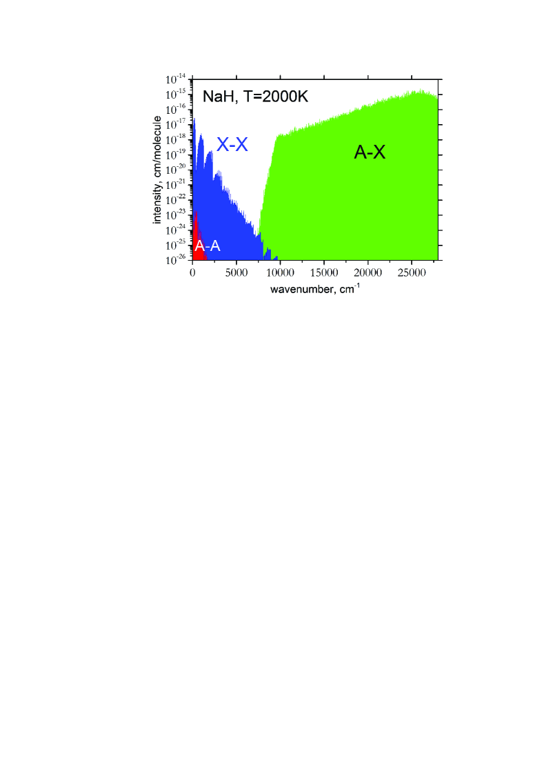
Figure 10: Overview of the absorption line intensities of NaH at $T$=2000 K computed using the line list of Rivlin et al. (2015).

5.5 Units

The default units of ExoCross are listed in Table 7. Microns ($\mu$m) can be optionally used for wavelength as alternative to wavenumber (default). Pressure does not have designated units; it is assumed to have the same units as of the parameter $P_{0}$ defining the broadening parameter $\gamma$, see Eq. (18).

Table 7: Units used by ExoCross 

Quantity	Units
Wavenumber	cm-1
Wavelength	$\mu$m
Temperature	K
Pressure	units of $P_{0}$
Absorption coefficient	cm$/$molecule
Absorption cross sections	cm$/$[molecule cm-1]
Emissivity	erg$/$s sr molecule
Specific heat	$JK^{-1}$ mol-1

5.6 Memory handling

The program records and controls the memory used at all processors. For proper control, the user is requested to specify the memory available on the machine in Gb or Mb. This number is used, for example, to estimate the number of transition lines from .trans processed simultaneously. At the end of the program a memory usage report is given.

6 Program repository

The ExoCross code together with manual and input examples are freely available from the ExoMol website , CCPForge or GitHub .

7 Conclusion

We present a new Fortran program ExoCross to compute different spectroscopic properties of molecules using spectral line lists. The program has being actively used by ExoMol to generate absorption cross sections using the ExoMol line lists available at www.exomol.com. In order to work with huge sizes of some line lists, ExoCross is optimized for efficient usage of parallelizm and vectorisation. Our new Voigt algorithm (Vectorized Voigt) is designed to be fast and accurate.

The program can easily be extended by users with their profiles or other functionality.

We are planning to provide production of $k$-coefficients as part of ExoCross in the future; integrate the API via the ExoMol .def file; reading the partition function from an ExoMol .pf file; implement a non-LTE model, which does not require definition of non-rigorous quantum numbers (see Section 2.11).

References

- Al-Refaie et al. (2015a) Al-Refaie, A. F., Ovsyannikov, R. I., Polyansky, O. L., Yurchenko, S. N., & Tennyson, J. 2015a, J. Mol. Spectrosc., 318, 84
- Al-Refaie et al. (2015b) Al-Refaie, A. F., Yachmenev, A., Tennyson, J., & Yurchenko, S. N. 2015b, MNRAS, 448, 1704
- Amundsen et al. (2014) Amundsen, D. S., Baraffe, I., Tremblin, P., et al. 2014, A&A, 564, A59
- Azzam et al. (2016) Azzam, A. A. A., Tennyson, J., Yurchenko, S. N., & Naumenko, O. V. 2016, MNRAS, 460, 4063
- Barber et al. (2006) Barber, R. J., Tennyson, J., Harris, G. J., & Tolchenov, R. N. 2006, MNRAS, 368, 1087
- Barton et al. (2014) Barton, E. J., Chiu, C., Golpayegani, S., et al. 2014, MNRAS, 442, 1821
- Barton et al. (2017) Barton, E. J., Hill, C., Yurchenko, S. N., et al. 2017, J. Quant. Spectrosc. Radiat. Transf., 187, 453
- Darby-Lewis et al. (2018) Darby-Lewis, D., Tennyson, J., Lawson, K. D., et al. 2018, J. Phys. B: At. Mol. Opt. Phys.
- Gamache et al. (2017) Gamache, R. R., Roller, C., Lopes, E., et al. 2017, J. Quant. Spectrosc. Radiat. Transf., 203, 70
- Goldenstein et al. (2017) Goldenstein, C. S., Miller, V. A., Spearrin, R. M., & Strand, C. L. 2017, Journal of Quantitative Spectroscopy and Radiative Transfer, 200, 249
- Gordon et al. (2017) Gordon, I. E., Rothman, L. S., Hill, C., et al. 2017, J. Quant. Spectrosc. Radiat. Transf., 203, 3
- Hill et al. (2013a) Hill, C., Gordon, I. E., Rothman, L. S., & Tennyson, J. 2013a, J. Quant. Spectrosc. Radiat. Transf., 130, 51
- Hill et al. (2013b) Hill, C., Yurchenko, S. N., & Tennyson, J. 2013b, Icarus, 226, 1673
- Humlicek (1979) Humlicek, J. 1979, J. Quant. Spectrosc. Radiat. Transf., 21, 309
- Jack et al. (2009) Jack, D., Hauschildt, P. H., & Baron, E. 2009, A&A, 502, 1043
- Jacquinet-Husson et al. (2016) Jacquinet-Husson, N., Armante, R., Scott, N. A., et al. 2016, J. Mol. Spectrosc., 327, 31
- Kochanov et al. (2016) Kochanov, R., Gordon, I., Rothman, L., et al. 2016, Journal of Quantitative Spectroscopy and Radiative Transfer, 177, 15 , xVIIIth Symposium on High Resolution Molecular Spectroscopy (HighRus-2015), Tomsk, Russia
- Lupu et al. (2016) Lupu, R. E., Marley, M. S., Lewis, N., et al. 2016, ApJ, 152, 217
- Malik et al. (2017) Malik, M., Grosheintz, L., Mendonça, J. M., et al. 2017, ApJ, 153, 56
- McKemmish et al. (2016) McKemmish, L. K., Yurchenko, S. N., & Tennyson, J. 2016, MNRAS, 463, 771
- Melnikov et al. (2016) Melnikov, V. V., Yurchenko, S. N., Tennyson, J., & Jensen, P. 2016, Phys. Chem. Chem. Phys., 18, 26268
- Min (2017) Min, M. 2017, A&A, 607
- Mizus et al. (2017) Mizus, I. I., Alijah, A., Zobov, N. F., et al. 2017, MNRAS, 468, 1717
- Müller et al. (2005) Müller, H. S. P., Schlöder, F., Stutzki, J., & Winnewisser, G. 2005, J. Molec. Struct. (THEOCHEM), 742, 215
- Neale et al. (1996) Neale, L., Miller, S., & Tennyson, J. 1996, ApJ, 464, 516
- Owens et al. (2017) Owens, A., Yurchenko, S. N., Yachmenev, A., Thiel, W., & Tennyson, J. 2017, MNRAS, 471, 5025
- Pavlyuchko et al. (2015) Pavlyuchko, A. I., Yurchenko, S. N., & Tennyson, J. 2015, MNRAS, 452, 1702
- Prajapat et al. (2017) Prajapat, L., Jagoda, P., Lodi, L., et al. 2017, MNRAS, 472, 3648
- Rey et al. (2016) Rey, M., Nikitin, A. V., Babikov, Y. L., & Tyuterev, V. G. 2016, J. Mol. Spectrosc., 327, 138
- Rivlin et al. (2015) Rivlin, T., Lodi, L., Yurchenko, S. N., Tennyson, J., & Le Roy, R. J. 2015, MNRAS, 451, 634
- Rothman et al. (2013) Rothman, L. S., Gordon, I. E., Babikov, Y., et al. 2013, J. Quant. Spectrosc. Radiat. Transf., 130, 4
- Rothman et al. (2010) Rothman, L. S., Gordon, I. E., Barber, R. J., et al. 2010, J. Quant. Spectrosc. Radiat. Transf., 111, 2139
- Rothman et al. (2005) Rothman, L. S., Jacquemart, D., Barbe, A., et al. 2005, J. Quant. Spectrosc. Radiat. Transf., 96, 139
- Rutkowski et al. (2018) Rutkowski, L., Foltynowicz, A., Johansson, A. C., et al. 2018, J. Quant. Spectrosc. Radiat. Transf., 205, 213
- Schreier (2017) Schreier, F. 2017, Journal of Quantitative Spectroscopy and Radiative Transfer, 187, 44
- Sharp & Burrows (2007) Sharp, C. M. & Burrows, A. 2007, ApJS, 168, 140
- Shine et al. (2012) Shine, K. P., Ptashnik, I. V., & Rädel, G. 2012, Surv. Geophys., 33, 535
- Showman et al. (2009) Showman, A. P., Fortney, J. J., Lian, Y., et al. 2009, ApJ, 699, 564
- Sousa-Silva et al. (2015) Sousa-Silva, C., Al-Refaie, A. F., Tennyson, J., & Yurchenko, S. N. 2015, MNRAS, 446, 2337
- Tennyson et al. (2014) Tennyson, J., Bernath, P. F., Campargue, A., et al. 2014, Pure Appl. Chem., 86, 1931
- Tennyson et al. (2013) Tennyson, J., Hill, C., & Yurchenko, S. N. 2013, in AIP Conference Proceedings, Vol. 1545, 6th international conference on atomic and molecular data and their applications ICAMDATA-2012 (AIP, New York), 186–195
- Tennyson et al. (2016a) Tennyson, J., Hulme, K., Naim, O. K., & Yurchenko, S. N. 2016a, J. Phys. B: At. Mol. Opt. Phys., 49, 044002
- Tennyson et al. (1993) Tennyson, J., Miller, S., & Le Sueur, C. R. 1993, Comput. Phys. Commun., 75, 339
- Tennyson & Yurchenko (2012) Tennyson, J. & Yurchenko, S. N. 2012, MNRAS, 425, 21
- Tennyson & Yurchenko (2017) Tennyson, J. & Yurchenko, S. N. 2017, Mol. Astrophys., 8, 1
- Tennyson et al. (2016b) Tennyson, J., Yurchenko, S. N., Al-Refaie, A. F., et al. 2016b, J. Mol. Spectrosc., 327, 73
- Underwood et al. (2016a) Underwood, D. S., Tennyson, J., Yurchenko, S. N., Clausen, S., & Fateev, A. 2016a, MNRAS, 462, 4300
- Underwood et al. (2016b) Underwood, D. S., Tennyson, J., Yurchenko, S. N., et al. 2016b, MNRAS, 459, 3890
- Wong et al. (2017) Wong, A., Yurchenko, S. N., Bernath, P., et al. 2017, MNRAS, 470, 882
- Yurchenko et al. (2017a) Yurchenko, S. N., Amundsen, D. S., Tennyson, J., & Waldmann, I. P. 2017a, A&A, 605, A95
- Yurchenko et al. (2016a) Yurchenko, S. N., Blissett, A., Asari, U., et al. 2016a, MNRAS, 456, 4524
- Yurchenko et al. (2016b) Yurchenko, S. N., Lodi, L., Tennyson, J., & Stolyarov, A. V. 2016b, Comput. Phys. Commun., 202, 262
- Yurchenko et al. (2018) Yurchenko, S. N., Sinden, F., Lodi, L., et al. 2018, MNRAS, 473, 5324
- Yurchenko & Tennyson (2014) Yurchenko, S. N. & Tennyson, J. 2014, MNRAS, 440, 1649
- Yurchenko et al. (2014) Yurchenko, S. N., Tennyson, J., Bailey, J., Hollis, M. D. J., & Tinetti, G. 2014, Proc. Nat. Acad. Sci., 111, 9379
- Yurchenko et al. (2017b) Yurchenko, S. N., Tennyson, J., & Barton, E. J. 2017b, J. Phys. Conf. Ser., 810, 012010