HFF-DeepSpace Photometric Catalogs of the Twelve Hubble Frontier Fields, Clusters and Parallels: Photometry, Photometric Redshifts, and Stellar Masses

Abstract

We present Hubble multi-wavelength photometric catalogs, including (up to) 17 filters with the Advanced Camera for Surveys and Wide Field Camera 3 from the ultra-violet to near-infrared for the Hubble Frontier Fields and associated parallels. We have constructed homogeneous photometric catalogs for all six clusters and their parallels. To further expand these data catalogs, we have added ultra-deep $K_{S}$-band imaging at 2.2 µm from the Very Large Telescope HAWK-I and Keck-I MOSFIRE instruments. We also add post-cryogenic Spitzer imaging at 3.6 µm and 4.5 µm with the Infrared Array Camera (IRAC), as well as archival IRAC 5.8 µm and 8.0 µm imaging when available. We introduce the public release of the multi-wavelength (0.2–8 µm) photometric catalogs, and we describe the unique steps applied for the construction of these catalogs. Particular emphasis is given to the source detection band, the contamination of light from the bright cluster galaxies and intra-cluster light. In addition to the photometric catalogs, we provide catalogs of photometric redshifts and stellar population properties. Furthermore, this includes all the images used in the construction of the catalogs, including the combined models of bright cluster galaxies and intra-cluster light, the residual images, segmentation maps and more. These catalogs are a robust data set of the Hubble Frontier Fields and will be an important aide in designing future surveys, as well as planning follow-up programs with current and future observatories to answer key questions remaining about first light, reionization, the assembly of galaxies and many more topics, most notably, by identifying high-redshift sources to target.

1. INTRODUCTION

Table 1Hubble Frontier Fields

Field	R.A.	Dec.	Cluster	Science Area	$F814W$ Area	$F160W$ Area	Name
	(h m s)	(d m s)	$z_{\mathrm{spec}}$	(arcmin2)	(arcmin2)	(arcmin2)
Abell 2744	00 14 21.20	$-$30 23 50.10	0.308	18.2	18.2	5.4	A2744-clu
Parallel	00 13 53.27	$-$30 22 47.80		11.9	11.9	5.0	A2744-par
MACS J0416.1-2403	04 16 8.38	$-$24 04 20.80	0.396	14.1	14.1	6.2	M0416-clu
Parallel	04 16 33.40	$-$24 06 49.10		11.9	11.9	5.0	M0416-par
MACS J0717.5+3745	07 17 34.00	$+$37 44 49.00	0.545	15.4	15.4	6.6	M0717-clu
Parallel	07 17 32.63	$+$37 44 59.70		13.0	12.9	6.5	M0717-par
MACS J1149.5+2223	11 49 35.43	$+$22 23 44.63	0.543	12.5	12.2	8.4	M1149-clu
Parallel	11 49 40.46	$+$22 18 01.53		14.3	14.3	5.3	M1149-par
Abell S1063	22 48 44.30	$-$44 31 48.40	0.348	14.6	14.6	5.9	A1063-clu
Parallel	22 49 17.80	$-$44 32 43.30		12.2	11.9	6.6	A1063-par
Abell 370	02 39 52.80	$-$1 34 36.00	0.375	15.1	13.8	8.3	A370-clu
Parallel	02 40 13.51	$-$1 37 34.00		11.9	11.9	5.0	A370-par

Note. — “Science Area” refers to the coverage area of the detection band (Section 3.3) in each field. We refer to the clusters and parallels by the names designated in “Name” throughout this work for simplicity.

Galaxy formation and evolution remain important topics of research in astronomy with many questions remaining. Large multi-wavelength photometric surveys have made it possible to study galaxy formation and evolution over most of cosmic time by observing large populations of galaxies. Recently, many surveys have leveraged ground- and space-based near-IR selected galaxy samples aimed to answer many topics from the build-up of the stellar mass function (e.g., Marchesini et al., 2009; Pérez-González et al., 2008; Muzzin et al., 2013a; Nantais et al., 2016; Song et al., 2016; Grazian et al., 2015; Tomczak et al., 2014), the star formation–mass relation (e.g. Whitaker et al., 2012; Duncan et al., 2014; Shivaei et al., 2015; Ly et al., 2015; Salmon et al., 2015), the structural evolution of galaxies (e.g., Franx et al., 2008; Bell et al., 2012; Wuyts et al., 2012b; van der Wel et al., 2012; Chang et al., 2013), star-formation histories of galaxies (Papovich et al., 2011; Pacifici et al., 2016; Tomczak et al., 2016; Webb et al., 2015; González et al., 2014), the formation of clusters (Muzzin et al., 2008, 2013c; Papovich et al., 2012; Hatch et al., 2016) and the stellar mass–metallicity relation (Tremonti et al., 2004; Wuyts et al., 2012a; Ly et al., 2015; Maier et al., 2015; Zahid et al., 2014; Yabe et al., 2012).

One recent effort to further our knowledge of galaxy formation and evolution is represented by the HST Frontier Fields (HFF) program (Lotz et al., 2017). The HFF program is a multi-cycle Hubble program consisting of 840 orbits of Director’s Discretionary (DD) time that imaged six fields centered on strong lensing galaxy clusters in parallel with six blank fields. Along with HST, the Spitzer Space Telescope has devoted 1000 hours of DD time to image the HFF fields at 3.6µm and 4.5µm with IRAC (Capak et al., in prep). The HFF combines the power of HST and Spitzer with the natural strong lensing gravitational telescopes of massive galaxy clusters to produce the deepest observations of clusters and their lensed galaxies ever obtained. We further include ultra-deep $K_{S}$ imaging from Keck and VLT (Brammer et al., 2016) and deep HST UV imaging (Siana et al., in prep) that bridges the UV to near-IR between the HST/ACS/WFC3 and Spitzer/IRAC imaging surveys. The HFF is further complemented by grism spectroscopy (GLASS Treu et al., 2015), deep far-IR imaging with Herschel (Rawle et al., 2016), 1.1 mm continuum detections from ALMA (González-López et al., 2017; Laporte et al., 2017), Chandra ACIS imaging (archival and additional program, PI C. Jones-Forman) and JVLA imaging (van Weeren et al., 2017), SCUBA-2 lensing cluster survey of radio-detected sub-mm galaxies (Hsu et al., 2017) and LMT (Pope et al., 2017), in addition to many ground-based photometric (Subaru and Gemini) and spectroscopic (MUSE, VLT, etc.) programs.

The six clusters $-$ Abell 2744, MACS J0416.1-2403, MACS J0717.5+3745, MACS J1149.5+2223, Abell S1063 and Abell 370 (for simplicity we designate a name for each field in Table 1) $-$ were selected based on their lensing strength, sky darkness, Galactic extinction, parallel field suitability, accessibility to ground-based facilities, HST, Spitzer and JWST observability, and pre-existing ancillary data. The primary science goals of the twelve HFF fields are to 1) reveal the population of galaxies at $z=5-10$ that are $10-50$ times intrinsically fainter than any presently known, 2) solidify our understanding of the stellar masses and star formation histories of faint galaxies, 3) provide the first statistically meaningful morphological characterization of star-forming galaxies at $z>5$, and 4) find $z>8$ galaxies magnified by the cluster lensing, with some bright enough to make them accessible to spectroscopic follow-up (Lotz et al., 2017).

The HFF poses many challenges akin to previous cluster surveys (e.g. CLASH Postman et al., 2012) due to the large fraction of light coming from the cluster itself. How does one preserve the information of the cluster galaxies but gain access to hidden/obscured background or underlying objects in the fields? The method most preferred is to model out the bright cluster galaxies (bCGs) dominating the majority of light. We define the term bCG to be “bright” cluster galaxy, as different from the traditional “brightest” cluster galaxy (BCG) terminology used in the literature, and hereafter refer to them as bCGs. There are various methods to accomplish this using GALFIT (Peng et al., 2010), IRAF and others (e.g., Connor et al., 2017; Merlin et al., 2016) to measure the light profiles of the bCGs and then subtract off the resulting model without destroying the background/underlying objects that are the reason for using the galaxy clusters as lenses. Specifically, the HFF are densely packed massive clusters from $0.3<z<0.6$ with dozens of bCGs that require modeling. Furthermore, the intra-cluster light (ICL) and bCGs light are entangled and need to be modeled together to appropriately remove the light they contribute to each image, which varies from band to band in each field (e.g., see Montes & Trujillo, 2014, for a study of the ICL). For a few fields in the HFF (e.g. M0416 cluster), this is further complicated by nearby bright galaxies that also must be modeled, if possible. Below, we discuss fully our approach and solutions to these challenges posed by the HFF observations.

We provide catalogs of photometric redshifts and stellar population properties for each field in the HFF, in addition to the photometric catalogs (similar to the ASTRODEEP collaboration Merlin et al., 2016; Castellano et al., 2016; Di Criscienzo et al., 2017, but utilizing different methodology). Furthermore, the public release is accompanied by all the images used in the construction of the catalogs, including the combined models of the bCGs and ICL, the residual images after bCG modeling, segmentation maps and more. The outline of the paper is as follows. In Section 2, we describe the datasets and data reduction steps performed. In Section 3, we describe our photometric methods, catalog format, flags and completeness, including a detailed description of our process for modeling out the bCGs (Section 3.1). In Section 4, we verify the quality and consistency of the catalogs. In Section 5, we describe the photometric redshift, rest-frame color, stellar population parameter fits to the SEDs and derived lensing magnifications. In Section 6, we summarize our data products and catalogs that have been generated of the HFF survey. We use the AB magnitude system throughout (Oke, 1971) and if necessary, a $\Lambda$CDM cosmology with $\Omega_{M}$ = 0.3, $\Omega_{\Lambda}$ = 0.7 and $H_{0}=70~{}$km s^-1 Mpc^-1.

2. DATA SETS

Table 2Image Sources

Field	Filters	Telescope/Instrument	Survey	Reference
A2744-clu	$F275W$, $F336W$	HST/UVIS	PID: 14209	PI: B. Siana
	$F435W$, $F606W$, $F814W$	HST/ACS	HFF	Lotz et al. (2017)
	$F105W$**, $F125W$, $F140W$**, $F160W$	HST/WFC3	HFF	Lotz et al. (2017)
	$K_{S}$	VLT/HAWK-I	KIFF	Brammer et al. (2016)
	3.6µm, 4.5µm, 5.8µm, 8.0µm	Spitzer/IRAC		see Section 2.2.2 for details
A2744-par	$F435W$, $F606W$, $F814W$	HST/ACS	HFF	Lotz et al. (2017)
	$F105W$**, $F125W$, $F140W$, $F160W$	HST/WFC3	HFF	Lotz et al. (2017)
	$K_{S}$	VLT/HAWK-I	KIFF	Brammer et al. (2016)
	3.6µm, 4.5µm	Spitzer/IRAC		see Section 2.2.2 for details
M0416-clu	$F225W$, $F390W$	HST/UVIS	CLASH	Postman et al. (2012)
	$F275W$, $F336W$	HST/UVIS	PID: 14209	PI: B. Siana
	$F435W$, $F606W$, $F814W$	HST/ACS	HFF	Lotz et al. (2017)
	$F475W$**, $F625W$**, $F775W$**	HST/ACS	PID: 12459	PI: M. Postman
	$F850LP$	HST/ACS	CLASH	Postman et al. (2012)
	$F105W$**, $F125W$**, $F140W$**, $F160W$**	HST/WFC3	HFF	Lotz et al. (2017)
	$F110W$**	HST/WFC3	CLASH	Postman et al. (2012)
	$K_{S}$	VLT/HAWK-I	KIFF	Brammer et al. (2016)
	3.6µm, 4.5µm	Spitzer/IRAC		see Section 2.2.2 for details
M0416-par	$F435W$, $F606W$, $F814W$	HST/ACS	HFF	Lotz et al. (2017)
	$F775W$**, $F850LP$**	HST/ACS	PID: 12459	PI: M. Postman
	$F105W$**, $F125W$, $F140W$, $F160W$	HST/WFC3	HFF	Lotz et al. (2017)
	$K_{S}$	VLT/HAWK-I	KIFF	Brammer et al. (2016)
	3.6µm, 4.5µm	Spitzer/IRAC		see Section 2.2.2 for details
M0717-clu	$F225W$, $F390W$	HST/UVIS	CLASH	Postman et al. (2012)
	$F275W$, $F336W$	HST/UVIS	PID: 14209	PI: B. Siana
	$F435W$, $F606W$, $F814W$	HST/ACS	HFF	Lotz et al. (2017)
	$F475W$**, $F625W$**, $F775W$**, $F850LP$**	HST/ACS	PID: 12103	PI: M. Postman
	$F555W$	HST/ACS	CLASH	Postman et al. (2012)
	$F105W$, $F125W$, $F140W$, $F160W$	HST/WFC3	HFF	Lotz et al. (2017)
	$F110W$	HST/WFC3	CLASH	Postman et al. (2012)
	$K_{S}$	Keck/MOSFIRE	KIFF	Brammer et al. (2016)
	3.6µm, 4.5µm	Spitzer/IRAC		see Section 2.2.2 for details
M0717-par	$F435W$, $F606W$, $F814W$	HST/ACS	HFF	Lotz et al. (2017)
	$F105W$, $F125W$, $F140W$, $F160W$	HST/WFC3	HFF	Lotz et al. (2017)
	$K_{S}$	Keck/MOSFIRE	KIFF	Brammer et al. (2016)
	3.6µm, 4.5µm	Spitzer/IRAC		see Section 2.2.2 for details
M1149-clu	$F225W$, $F390W$	HST/UVIS	CLASH	Postman et al. (2012)
	$F275W$, $F336W$	HST/UVIS	PID: 14209	PI: B. Siana
	$F435W$, $F606W$, $F814W$	HST/ACS	HFF	Lotz et al. (2017)
	$F475W$, $F555W$, $F625W$, $F775W$, $F850LP$	HST/ACS	CLASH	Postman et al. (2012)
	$F105W$, $F125W$, $F140W$, $F160W$	HST/WFC3	HFF	Lotz et al. (2017)
	$F110W$	HST/WFC3	CLASH	Postman et al. (2012)
	$K_{S}$	Keck/MOSFIRE	KIFF	Brammer et al. (2016)
	3.6µm, 4.5µm	Spitzer/IRAC		see Section 2.2.2 for details
M1149-par	$F435W$, $F606W$, $F814W$	HST/ACS	HFF	Lotz et al. (2017)
	$F105W$, $F125W$, $F140W$, $F160W$	HST/WFC3	HFF	Lotz et al. (2017)
	$K_{S}$	Keck/MOSFIRE	KIFF	Brammer et al. (2016)
	3.6µm, 4.5µm	Spitzer/IRAC		see Section 2.2.2 for details
A1063-clu	$F225W$, $F390W$	HST/UVIS	CLASH	Postman et al. (2012)
	$F275W$, $F336W$	HST/UVIS	PID: 14209	PI: B. Siana
	$F435W$, $F606W$, $F814W$	HST/ACS	HFF	Lotz et al. (2017)
	$F475W$, $F625W$, $F775W$, $F850LP$	HST/ACS	CLASH	Postman et al. (2012)
	$F105W$, $F125W$, $F140W$, $F160W$	HST/WFC3	HFF	Lotz et al. (2017)
	$F110W$**	HST/WFC3	PID: 12458	PI: M. Postman
	$K_{S}$	VLT/HAWK-I	KIFF	Brammer et al. (2016)
	3.6µm, 4.5µm, 5.8µm, 8.0µm	Spitzer/IRAC		see Section 2.2.2 for details
A1063-par	$F435W$, $F606W$, $F814W$	HST/ACS	HFF	Lotz et al. (2017)
	$F105W$, $F125W$, $F140W$, $F160W$	HST/WFC3	HFF	Lotz et al. (2017)
	$K_{S}$	VLT/HAWK-I	KIFF	Brammer et al. (2016)
	3.6µm, 4.5µm	Spitzer/IRAC		see Section 2.2.2 for details
A370-clu	$F275W$, $F336W$	HST/UVIS	PID: 14209	PI: B. Siana
	$F435W$, $F606W$, $F814W$	HST/ACS	HFF	Lotz et al. (2017)
	$F475W$**, $F625W$**	HST/ACS	PID: 11507	PI: K. Noll
	$F475W$**	HST/ACS	PID: 11582	PI: A. Blain
	$F625W$**	HST/ACS	PID: 13790	PI: S. Rodney
	$F105W$, $F125W$, $F140W$, $F160W$	HST/WFC3	HFF	Lotz et al. (2017)
	$F110W$**	HST/WFC3	PID: 11591	PI: J.P. Kneib
			PID: 13790	PI: S. Rodney
	$K_{S}$	VLT/HAWK-I	KIFF	Brammer et al. (2016)
	3.6µm, 4.5µm, 5.8µm, 8.0µm	Spitzer/IRAC		see Section 2.2.2 for details
A370-par	$F435W$, $F606W$, $F814W$	HST/ACS	HFF	Lotz et al. (2017)
	$F105W$, $F125W$, $F140W$, $F160W$	HST/WFC3	HFF	Lotz et al. (2017)
	$K_{S}$	VLT/HAWK-I	KIFF	Brammer et al. (2016)
	3.6µm, 4.5µm	Spitzer/IRAC		see Section 2.2.2 for details

Note. — HST/ACS and HST/WFC3-IR bands marked by (**) are processed internally by our group to improve and/or include any additional data that is available (see Section 2.1.2).

The twelve Hubble Frontier Fields (HFF) have been observed with HST/WFC3, HST/ACS (Lotz et al., 2017), Spitzer and two ground-based observatories (VLT and Keck-I) for added ultra-deep $K_{S}$-band imaging (Brammer et al., 2016). In each field, the data consist of the ACS $F435W$, $F606W$, $F814W$ and WFC3 $F105W$, $F125W$, $F140W$, $F160W$ images obtained from the HFF Program. In this section, we describe our data reduction steps and summarize all other space- and ground-based data that are used to construct the catalogs.

The photometric catalogs make use of 22 filters (see Table 2) and corresponding image mosaics from not only the HFF program but previous programs that have observed the HFF fields (e.g. CLASH Postman et al., 2012). We projected all $Hubble$ data onto the astrometric grid and pixel scale defined in the data released products for the HFF Program, specifically the $F160W$ filter, but allowing for larger coverage areas from the additional data (i.e. Abell 2744 cluster, hereafter A2744-clu, see Table 1).

2.1. Hubble Frontier Fields Imaging

2.1.1 Sources of Data

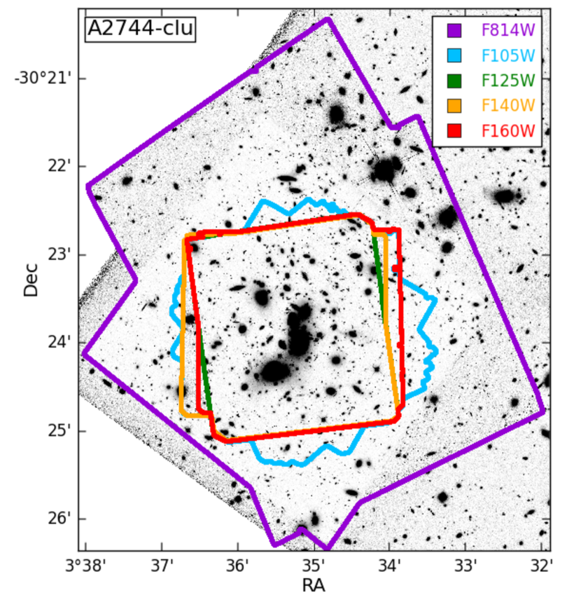
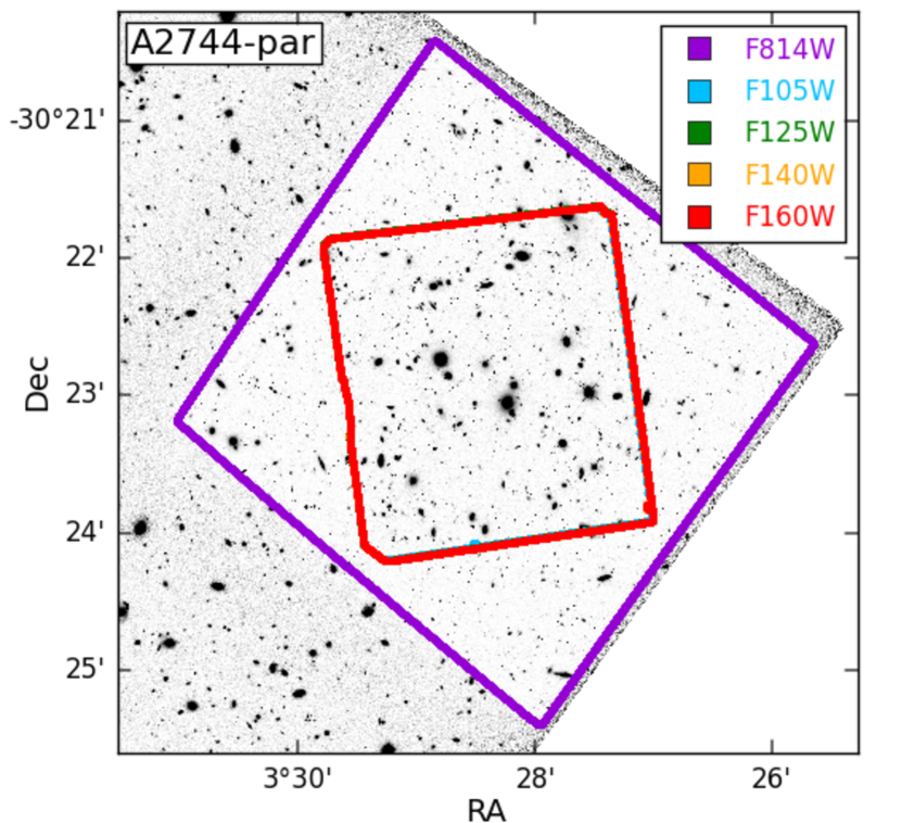
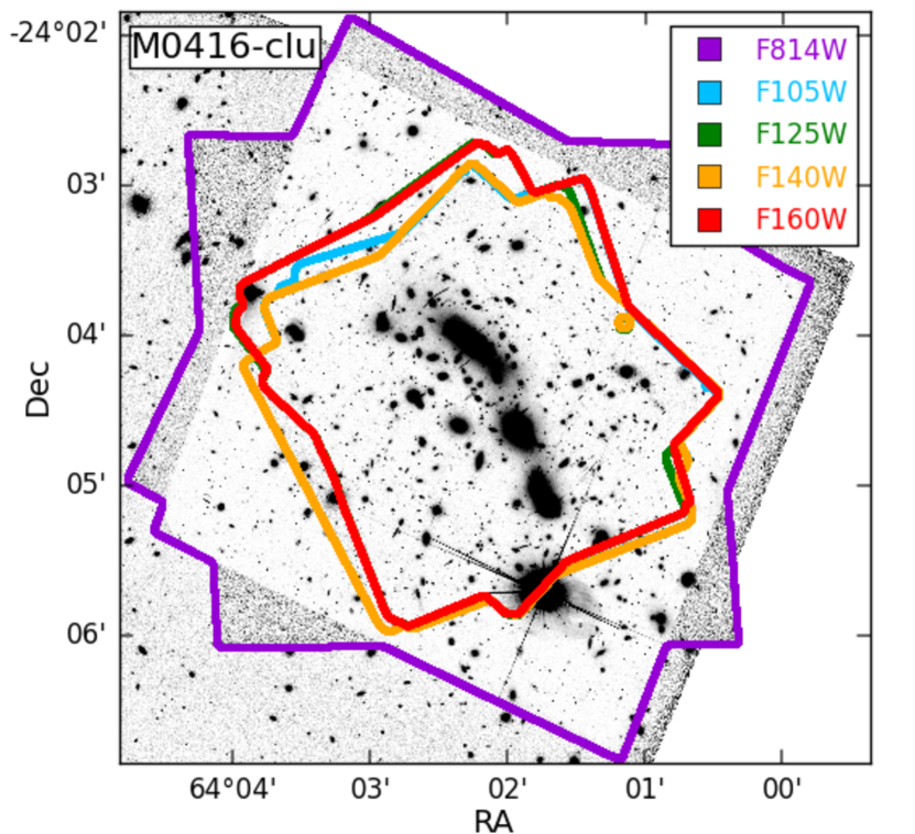
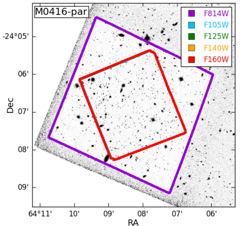
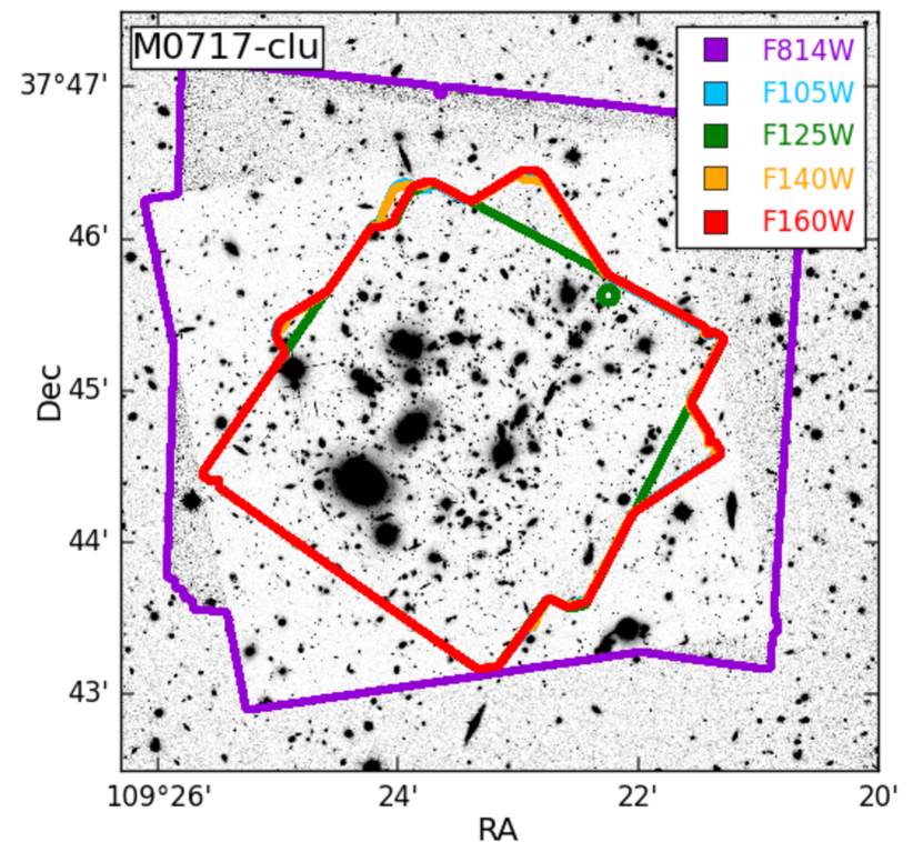
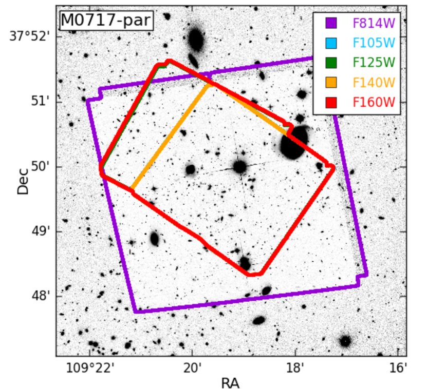
Figure 1.— Layout of the Hubble observations used. The catalogs presented here cover the entire area encompassed by the five bands ($F814W$, $F105W$, $F125W$, $F140W$, $F160W$; i.e. the detection band, see Section 3.3). The imaging is of the $F814W$ band inside its border and the $K_{S}$ band outside of it. North is up and East is to the left.

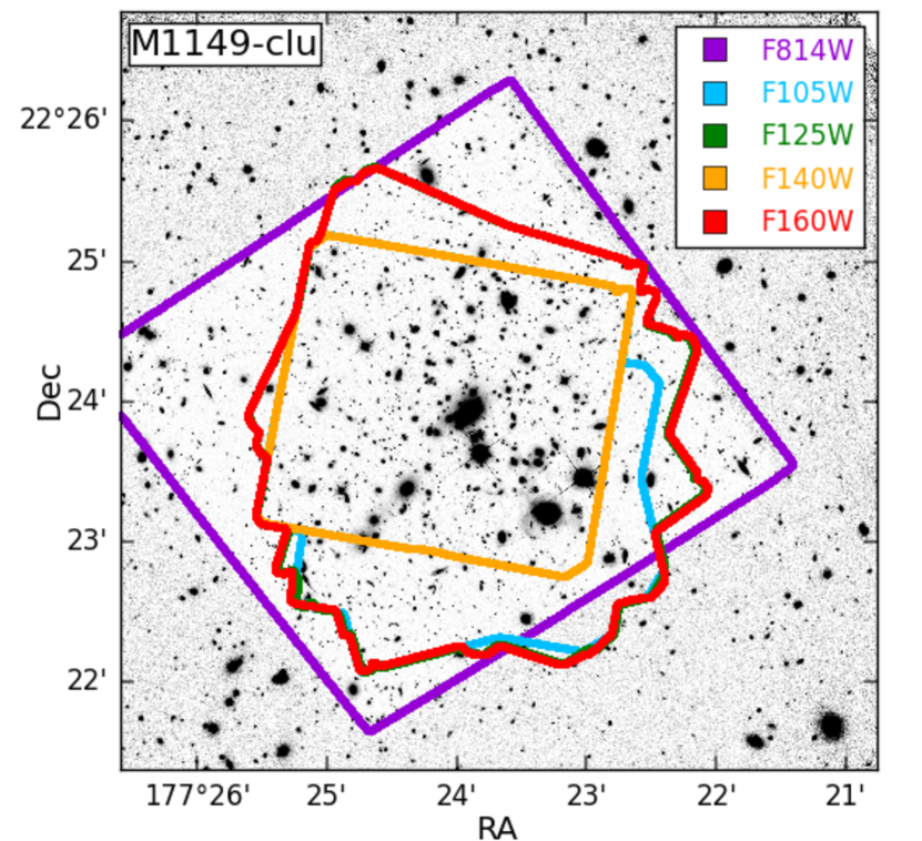
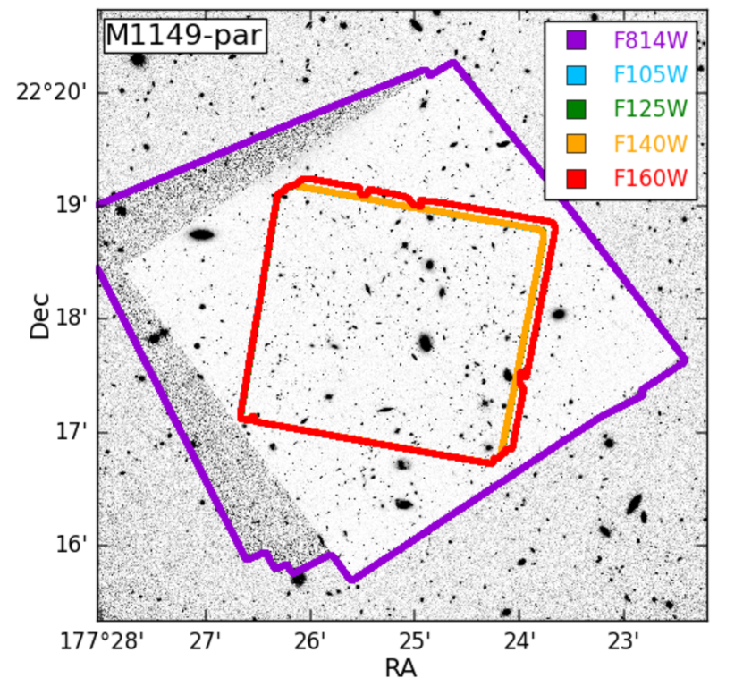
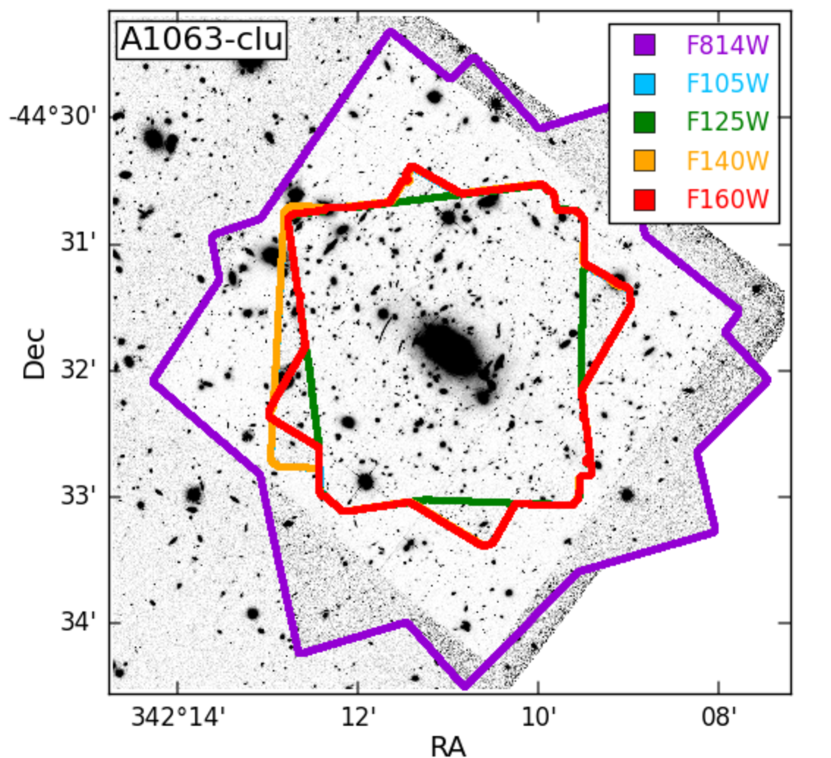
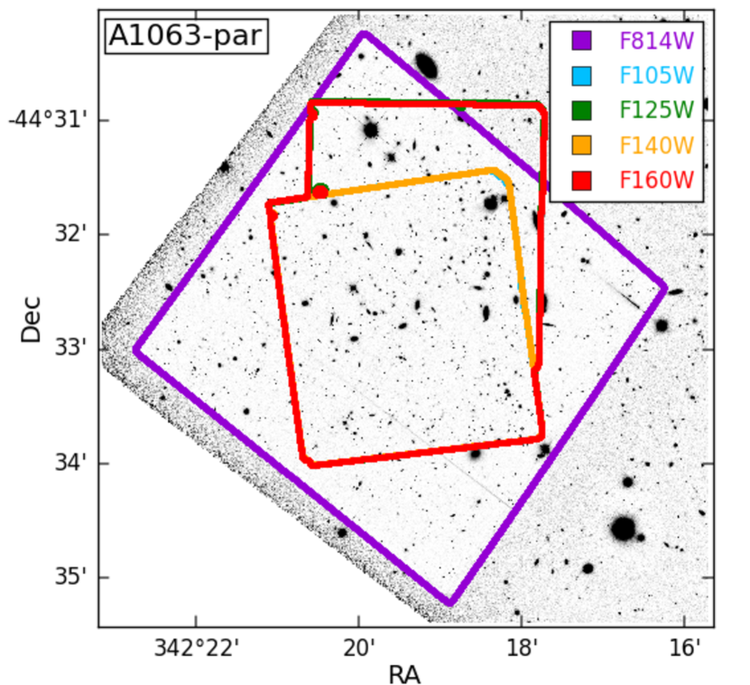
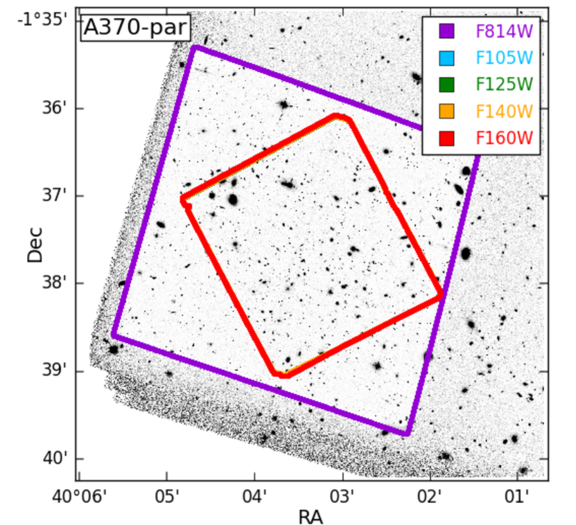
Figure 2.— Same as Figure 1 of the last 3 cluster and parallel fields observed (labeled in plot).

To maximize the depth and coverage of the Hubble Frontier Fields, we collected imaging from any previous HST observations utilizing the ACS and WFC3 instruments for any of the 17 filters in our catalogs. The coordinates and coverage areas of all twelve fields’ catalogs are given in Table 1. The “Science Area” column indicates the region covered by the $F814W$, $F105W$, $F125W$, $F140W$ and $F160W$ bands (i.e. the detection band, see Section 3.3). Other HST programs have carried out observations of the HFF and we have incorporated these additional data sets into our mosaics for each field, where available, to increase the depth and area coverage of the catalogs (see Table 2). Furthermore, CLASH and other smaller surveys of the HFF have added filters beyond those observed with the HFF Program albeit to shallower depths.

All near-IR HST observations are obtained using the Wide Field Camera 3 IR detector (WFC3/IR), which has a $1024\times 1024$ HgCdTe array. The usable portion of the detector is $1014\times 1014$ pixels, covering a region of $136\arcsec\times 123\arcsec$ across with a native pixel scale of $0\farcs 128$ pixel^-1 (at the central reference pixel). The HFF observations are done in four wide filters: $F105W$, $F125W$, $F140W$ and $F160W$, which cover the wavelength ranges of $\sim 0.9\micron-1.2\micron$, $\sim 1.1\micron-1.4\micron$, $\sim 1.2\micron-1.6\micron$ and $\sim 1.4\micron-1.7\micron$, respectively. The standard designations for the four filters are $Y_{F105W}$, $J_{F125W}$, $JH_{F140W}$ and $H_{F160W}$, however we will refer to them by the HST filter name to avoid confusion with ground-based bandpasses. The available UV data are obtained using the WFC3/UVIS detector which has two $2051\times 4096$ UV optimized e2v CCDs. The usable portion of the detector is rhomboidal, covering a region of $162\arcsec\times 162\arcsec$ across with a native pixel scale of $0\farcs 04$ pixel^-1 (at the central reference pixel).

All visible HST observations are obtained using the Advanced Camera for Surveys WFC detector (ACS/WFC), which has two $2048\times 4096$ SITe CCDs array. The usable portion of the detector is $4040\times 4040$ pixels, covering a region of $202\arcsec\times 202\arcsec$ across with a native pixel scale of $0\farcs 049$ pixel^-1 (at the central reference pixel). The HFF observations are done in three wide filters: $F435W$, $F606W$ and $F814W$, which cover the wavelength ranges of $\sim 0.35\micron-0.5\micron$, $\sim 0.5\micron-0.7\micron$ and $\sim 0.7\micron-0.95\micron$, respectively. The standard designations for the three filters are $B_{F435W}$, $V_{F606W}$ and $I_{F814W}$, however we will refer to them by the HST filter name to avoid confusion.

2.1.2 Data Reduction

We downloaded the HST science and weight images for each available filter of the HFF fields following the observational scheduled defined by the program. The HFF images downloaded are the latest version available (v1.0 in all cases; Koekemoer et al., in prep). Other HST images covering the HFF fields are downloaded from the MAST archive. In a few cases, this required that we process some of the HFF filter images internally when additional data is available. We designate these bands in Table 2. We downloaded CLASH archival science and weight images during February 2015. All data images used are constructed from the best available data pipelines at the time. Before modeling out the bCGs in each field (see Section 3.1), data reduction steps are performed to prepare the science and weight images for modeling. We describe these steps in the following paragraphs.

The final mosaics in each filter for the HFF Program release are stacked and drizzled image products at 30 and 60 mas pixel scales, with major artifacts removed. All images are aligned to the same astrometric grid based on previous HST and ground-based catalogs (see Lotz et al., 2017, for further information). We use the 60 mas pixel scale ($0\farcs 06$/pix) images in our analysis for catalog construction as this was the most reasonable for all accompanying data products. The CLASH  image products are produced similarly but at 30 and 65 mas pixel scales. We chose the 30 mas images and use the IRAF tool WREGISTER to match the CLASH images to the 60 mas pixel scale HFF images. In a few cases, we process some of the CLASH filter images internally when additional data is available or to improve the mosaics (designated in Table 2).

For additional HST data images that have not been through the HFF or CLASH data release pipelines, these images are produced with AstroDrizzle to create the science and weight images from the FLT and ASN files from the MAST archive. In order to exactly match the pixel scale ($0\farcs 06$), we use the $F160W$ filter image from the HFF Program as a reference image for AstroDrizzle in each field. Deeper WFC3/UVIS $F275W$ and $F336W$ data have been collected by the HST observing program PID: 14209 (PI: B. Siana). We reduce these data internally and the produced mosaics are processed further similarly to the other HST bands. At this point, we have produced data images for all HST filters, of each field, that we include in the final catalogs and match the released HFF images at a pixel scale of $0\farcs 06$. The remaining data reduction and analysis steps are the same for all HST and $K_{S}$ band images (see Section 2.2.1).

A background subtraction is performed on each science image for each field using a Gaussian interpolation to smooth out the mosaic and remove sky background. The Gaussian interpolation is performed by sampling the mosaics in small regions (size of region defined arbitrarily based on results of interpolation) and setting a limiting magnitude and threshold of sources that can contribute to the overall background of the image. For the HST images and $K_{S}$ band, we found SExtractor AUTO background subtraction runs best with the following parameters: mesh size of 64, limiting magnitude of 15 and maximum threshold of 0.01. If there are multiple epochs for the same field and filter, we combine the background-subtracted mosaics using a weighted mean and simply add the weight images together.

Next, we improve the mosaics for modeling and catalog construction by detecting and cleaning cosmic rays that remain after the initial AstroDrizzle combination. It is important to remove cosmic rays so that they are not detected as sources and to not affect the nearby pixels once we have point-spread function (PSF)-matched images. We remove any cosmic rays either by hand using a DS9 region mask or by running the image through, L.A. Cosmic (van Dokkum, 2001). This step improves the image quality and reduces the number of false detections.

The final step we perform, before we model out the bCGs, is to remove any data that would been seen as bad data during the modeling process. This is accomplished by creating a weight mask for each filter of each field. We mask any pixel whose value in the weight image is very small compared to the median weight of the image. The value of the weight pixels should never be negative and ones that have very small values typically have shorter exposure times and have unacceptable science data quality necessary for analysis. These background subtracted, cosmic ray cleaned, and weight masked images are now ready to be used for the modeling of the bCGs (see Section 3.1).

2.2. Additional Data

For better and more complete photometric catalogs of the HFF, we collect additional data available from ground-based sources ($K_{S}$-band imaging, 2.2µm) and Spitzer/IRAC (3.6µm and 4.5µm imaging, also 5.8µm and 8.0µm imaging is available for the three Abell clusters) to extend the coverage of these fields into the IR. The sources of the additional data are described in the following sections. The raw $K_{S}$-band images were drizzled to $0\farcs 06$ pixel scale to match the HST image grid and the Spitzer/IRAC imaging pixel scale is $5\times$ larger ($0\farcs 3$). We describe the modeling and analysis of these data sets in Section 3.1.4.

2.2.1 $K_{S}$-band Imaging

Ultra-deep $K_{S}$ imaging of all of the HFF clusters and parallels were carried out for the “$K$-band Imaging of the Frontier Fields” (“KIFF”) project (Brammer et al., 2016). These observations have been observed with the VLT/HAWK-I and Keck/MOSFIRE instruments for the six clusters and six parallel fields. The VLT/HAWK-I integrations of the A2744, M0416, A1063 and A370 clusters and parallels reach 5$\sigma$ limiting depths of $K_{S}\sim 26.0$ (AB, point sources) and have excellent image quality (FWHM $\sim 0\farcs 4$). Shorter Keck/MOSFIRE integrations of the M0717 and M1149 clusters and parallels reach limiting depths $K_{S}=25.5$ and 25.1 with seeing FWHM$\sim 0\farcs 4$ and $0\farcs 5$, respectively. In all cases, the $K_{S}$-band mosaics cover the primary cluster and parallel HFF fields entirely with small exceptions (see Figures 1 and 2). The total area of the $K_{S}$-band imaging is 490 arcmin². These observations (at 2.2µm) fill a crucial gap between the space-based observations of the HFF (reddest HST filter, 1.6 µm) and Spitzer/IRAC (bluest 3.6 µm). While not as deep as the space-based observations, these deep $K_{S}$-band images provide important constraints in determining galaxy properties from galaxy modeling that are improved greatly from this extra coverage (see Brammer et al., 2016, for more detail).

2.2.2 $IRAC$ Imaging

The multi-wavelength photometric catalogs presented in this work include photometry in the Spitzer/IRAC 3.6 µm and 4.5 µm bands based on the full-depth mosaics assembled by our group. These data probe rest-frame wavelengths redder than the Balmer Break up to $z\sim 8-10$, and therefore provide important constraints for the derived photometric redshift and stellar population parameters.

The IRAC 3.6 µm and 4.5 µm mosaics combine all the Spitzer/IRAC data available to December 2016. Specifically, A2744 and its parallel are combined data from PID 83 (PI: Rieke) and PID 90257 (PI: Soifer); M0416 and its parallel from PID 90258 (PI: Soifer) and PID 80168 (ICLASH - PI: Bouwens); M0717 and its parallel from PID 90259 (PI: Soifer), PID 60034 (PI: Egami) and PID 90009 (SURFS-UP - PI: Bradac); M1149 and its parallel from PID 90260 (PI: Soifer), PID 60034 (PI: Egami) and PID 90009 (SURFS-UP - PI: Bradac); A1063 and its parallel from PID 10170 (PI: Soifer), PID 83 (PI: Rieke), and PID 60034 (PI: Egami); finally, A370 and its parallel from PID 10171 (PI: Soifer), PID 64 (PI: Fazio), PID 137 (PI: Fazio) and PID 60034 (PI: Egami).

Notably, A2744, A1063 and A370 clusters benefit from observations of the IRAC 5.8 µm and 8.0 µm bands during the cryogenic mission (PIDs 83, 64 and 137). Mosaics in these bands are built using the same procedures adopted for the IRAC 3.6 µm and 4.5 µm bands. Below, we introduce briefly the steps adopted to assemble the IRAC mosaics, referring the reader to Labbé et al. (2015) for a more detailed description of the process.

The reduction of the IRAC data is carried out using the pipeline developed by Labbé et al. (2015), using the corrected Basic Calibrated Data (cBCD) generated by the Spitzer Science Center (SSC) calibration pipeline. The full process is organized in two passes. During the first pass, each cBCD frame is corrected for background and persistence from very bright stars and other artifacts. Then the frames of each Astronomical Observation Request (AOR) are registered to the reference frame (the HFF detection image) and median combined. During the second pass, the pipeline removes cosmic rays, improves the background subtraction and carefully aligns the frames to the reference image, before the final co-addition of the frames. The resulting mosaics have a pixel scale of $0\farcs 3$ and the same tangential point of the HFF detection image. The average exposure in the 3.6 µm and 4.5 µm is $\sim 50h$, corresponding to an AB magnitude depth of $\sim 25$ ($5\sigma$, aperture $3\farcs 0$ diameter). In all cases, the IRAC imaging for the 3.6 µm and 4.5 µm bands cover the primary cluster and parallel fields entirely of the HFF.

Accurate PSFs are key for robust photometry. For each mosaic, the pipeline generates a spatially varying empirical PSF. At each position in a grid across the mosaic, a high signal-to-noise (S/N) template PSF, obtained from observations of $\sim 200$ stars, is rotated and weighted according to the rotation angles and exposure time map of each AOR at the specific position on the grid. The final PSF is constructed combining the set of rotated, weighted templates.

3. Photometry

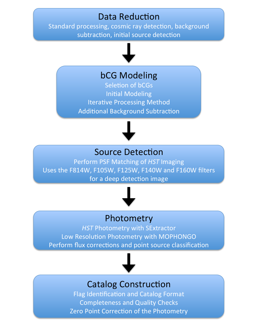
Figure 3.— Illustration of the main steps performed from data reduction to final catalog construction for all the data presented here of the HFF cluster and parallel fields.

Here, we describe the procedure for producing the photometric catalogs of each field. We start by following the standard pipeline for image processing, performing background subtraction on each image before combining multiple epochs (if already not performed by the HFF data core team) and cleaning the images for remaining artifacts and cosmic rays (Section 2.1.2). Next, we model out bCGs from each field that contribute significant light and perform an additional background subtraction on the resulting bCGs out mosaics (Section 3.1). We then PSF match the shorter wavelength bands to the WFC3/$F160W$ band and perform a source detection with SExtractor for each field using a detection image created from the $F814W$, $F105W$, $F125W$, $F140W$ and $F160W$ bands (Section 3.3). Finally, fluxes are estimated for each band of each field with SExtractor and error analysis is performed (Section 3.5). We show a diagram of the procedure in Figure 3.

3.1. Modeling Out of bCGs

One of our main science goals for these catalogs is to identify sources magnified by the gravitational potential of the cluster galaxies and the cluster itself. To accomplish this, we need to model out the light from the galaxy cluster members or at least the brightest members that contribute the most light to the cluster and ICL. We adopt a method that measures the isophotal parameters of a galaxy and removes the resulting model as described by Ferrarese et al. (2006). We summarize the procedure and additions necessary for our modeling purposes. In the following sections, we describe our selection of bCGs that contribute significantly to the light of the cluster. We summarize the procedure that creates a galaxy model for a bCG. Finally, we describe our iterative process that improves on the initial models to produce a final cluster model.

3.1.1 Selection of bCGs

As a first pass, we identify bCGs to be modeled out using an over-subtracted background detection image to produce a segmentation map and associated initial catalog. This detection image is constructed in the same manner that is performed for our final catalogs (Section 3.3). This is accomplished using SExtractor with an aggressive background subtraction to identify the centers of all sources and have a complete as possible initial catalog (Figure 4, left panel).

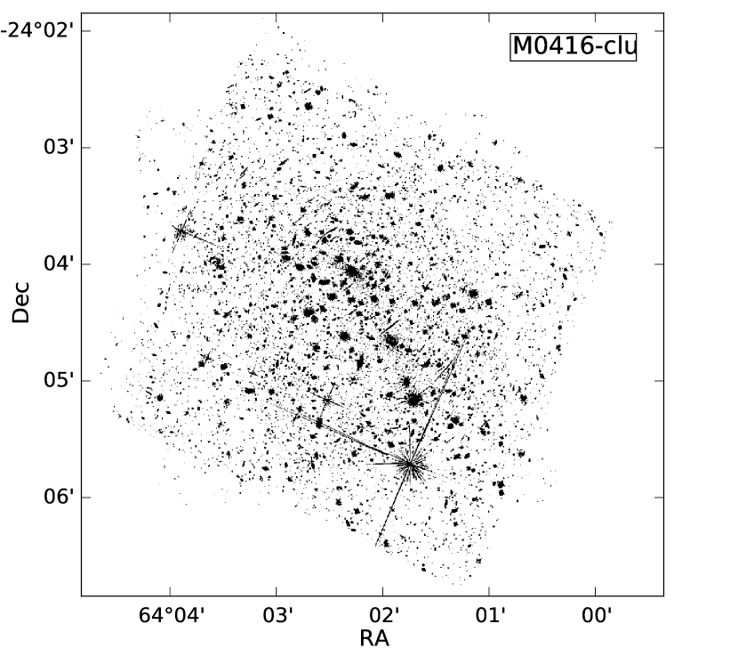
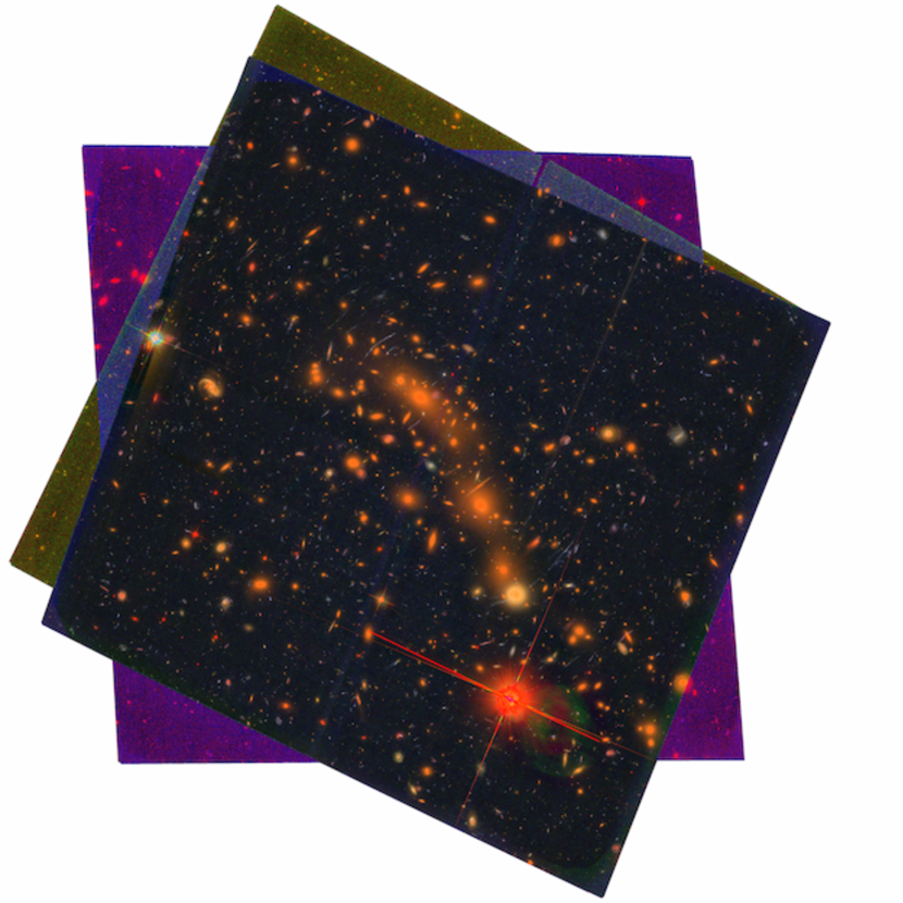
Figure 4.— (Left panel) Initial segmentation map of M0416 cluster using a heavy background subtraction with SExtractor for identifying bCGs to be modeled out (all other fields can be found in the Appendix). North is up and East is to the left. (Right panel) A false color RGB image of the cluster made with the $F435W$, $F606W$ and $F814W$ bands to better identify cluster members (reddish-orange colored galaxies; refer to Section 3.1.1 for further details).

We take great care to identify cluster members by color with RGB mosaics of each field (cluster members appear as reddish-orange galaxies, right panel of Figure 4). We create the RGB mosaics of each field using the $F435W$, $F606W$ and $F814W$ bands. These bands are chosen to limit the light from the brightest galaxies that would wash out the detail to identify smaller contributing cluster members affecting our ability to identify background sources. Ultimately, the selection of cluster members to be modeled out is done in a somewhat arbitrary manner but guided by the principals that these galaxies are bright and/or affecting nearby background sources and appear in many bands for better modeling. For these reasons, we are more aggressive in our selection of bCGs to model out that fall within the WFC3 footprint and less aggressive outside the WFC3 footprint (i.e. the ACS). Also, we choose to model out fainter cluster members that have lensed sources nearby that affect their photometry.

Furthermore, due to the limitations of the modeling code to handle nearby resolved spiral galaxies, we choose not to model them out (even if the source contributes significantly to the light in the field) as the resulting residual and model are undesirable. However, we do model out nearby bright elliptical galaxies when possible (e.g. M0416 and M0717 clusters), but this results in only a few galaxies for all fields. Also, we limit our selection to not include edge-on disk galaxies of cluster members due to these limitations (see Ferrarese et al., 2006, Section 3.2 for specifics). However, we do note a few edge-on galaxies are selected, where the benefit of modeling out the galaxy improves the detection of background sources.

3.1.2 Method for Modeling a bCG

We summarize here the method used to model a galaxy’s light of our selected sources (we refer the reader to Ferrarese et al., 2006, for more detailed information on the modeling procedure) and describe changes to this code that are necessary for the HFF data. Again, we note that this code is designed originally to model elliptical galaxies and has some shortcomings for spiral galaxies. However, our improvements using an iterative process have made these shortcomings mostly negligible (see Section 3.1.3). Furthermore, the adopted method is superior compared to other modeling codes, e.g. GALFIT, especially for elliptical galaxies with significant isophotal twisting, which are the predominant type of bright galaxies in the cluster environment and those limiting the full exploitation of the HFF cluster data depth.

The IRAF task ELLIPSE is used to measure the isophotal parameters for each modeled galaxy. The best fitting parameters are determined by minimizing the sum of the squares of the residuals between the data and the ellipse model. First, a mask is created that masks all sources but the galaxy to be modeled. This is done using SExtractor to identify all possible sources in the mosaic of the band. Next, all objects near the center of the bCG are unmasked and an ELLIPSE run is performed with a fixed center. SExtractor is run again on the residual image using a weight image (which prevents it from picking up noisy areas and residuals) to create a mask of objects near the bCG. The final mask is built from the first mask outside a region determined by the ELLIPSE run and the new mask inside. Finally, the central region of the bCG is unmasked and then the mask is blurred, by a Gaussian profile, to minimize pixels that may have been missed during this process.

The next step is to create the model itself. This is accomplished by using the mask created and performing another ELLIPSE run with all parameters allowed to vary (including the center within 2 pixels). The surface brightness parameters are found out to a radius we set arbitrarily, but large enough to measure all the light of the bCG, and this can include ICL. However, ELLIPSE fails to converge well before this condition is met. When this happens, the mean values for the five outermost fitted isophotes are calculated and ELLIPSE is run with $\theta$, $\epsilon$ and the isophotal center fixed to these values. The parameters that are returned from this procedure are given to the IRAF task BMODEL to create the model from the isophotal parameters. However, BMODEL can have problems getting the interpolation correct, especially at large radii, with spurious results. This is fixed by splining and interpolating the parameters from the ELLIPSE run that is used for BMODEL. Furthermore, a local background, for the extent of the bCG model, is estimated and added to produce the final model for the bCG. This results in a more accurate residual and a smoother profile at larger radii.

Finally, the curve of growth is measured from the largest radii isophote inwards to determine when the model surface brightness falls below the measured sky background for the image. This is done to help eliminate extra light being modeled that is attributed to the sky. The resulting built model for the bCG is then subtracted from the mosaic. We create an input list of all the galaxies that we have selected to be modeled and do an initial run for each galaxy. This is done in succession for each galaxy to be modeled creating a new mosaic with the galaxy removed. We manually check the final result after all the bCGs have been modeled out to see if manual input is required.

We make an addition to the galaxy modeling code by creating a “master mask” from the original mosaic to be used for each bCG modeled out. We make the master mask in the same manner as described previously in this section, but all sources are masked. Then for each bCG modeled out, we use the master mask and substitute in a small portion (a box) of the mask created for the bCG being modeled out. We substitute mask sizes of $3\farcs 6-24^{\prime\prime}$ along a side as determined by the size of the bCG and density of nearby sources. We add this step because the mask created for the bCG can be affected by residuals from poor modeling of previous bCGs, negatively impacting nearby sources and subsequent modeling. We discuss the importance of this step further in the iterative process (Section 3.1.3).

We find the procedure for the modeling of a bCG works quite well in an automated way. But, one aspect that has significant impact requiring manual input for some bCGs is to edit the mask manually, usually masking more area around other nearby sources contributing to the fit. This is accomplished using the IRAF task IMEDIT. When this occurs, the mask is saved and used for all future runs as explained further in the iterative process.

3.1.3 Iterative Processing Method of bCGs

The initial model of the cluster for each band (sum of all modeled bCGs that includes ICL; see Table 3 for number of bCGs modeled in each field) is a useful result but not very accurate for precise photometry of the remaining sources or reliable photometry of the bCGs themselves (see panels second from left in Figure 5). To improve the models themselves and thus improve the photometry, we developed an iteration method that can be run on the resulting models to improve them. For clarity, we define the term “original mosaic” as the mosaic created after the data reduction steps discussed earlier but before any bCG modeling has been performed (including the initial run).

Table 3bCGs Modeled for Each Field

Field	Cluster	Parallel
	(# Galaxies)	(# Galaxies)
A2744	79	27
M0416	49	12
M0717	35	7
M1149	63	9
A1063	90	22
A370	75	13

Note. — The number of bCGs is for the $F814W$ filter and includes all bCGs that were modeled for that field. The same amount or less were modeled out for each of the other filters from the same set of bCGs.

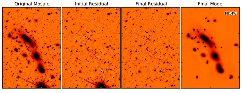
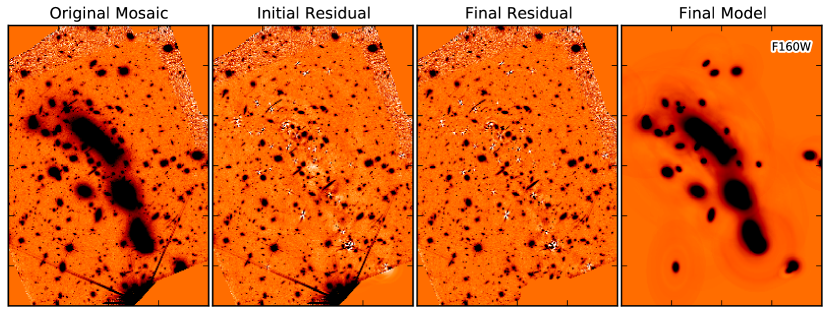
Figure 5.— Results from the modeling procedure on the M0416 cluster $F814W$ (top) and $F160W$ (bottom) bands (all other fields can be found in the Appendix). Left to right: The original image (defined in Section 3.1.3), residual mosaic after the initial run (Section 3.1.2), final mosaic after the additional sky subtraction (Section 3.2) and model of the cluster after iterative processing method (Section 3.1.3). All images show the same scale and region of the cluster. The final residual mosaic is used to extract the photometry of all detected sources except for the modeled out bCGs, whose photometry is extracted from the final model image.

After the initial run (described above), the code runs through 10 more iterations of each galaxy in the input list of bCGs for the specific field and band (11 total iterations). For the first iteration (modeling the bCGs for the second time) we start with the residual image after all the galaxies have been modeled out (i.e. the resulting mosaic after the initial run). Then, in succession, we add back each bCG modeled out one at a time to this residual image (in effect creating a new mosaic with only that bCG included) and re-run the modeling of it. We then subtract off the new model from this image where the previous model was added back into it. The result of this improves the model and the residual for that bCG without having contamination from all the surrounding bCGs that hindered the initial models. This is done for all the galaxies in the input list until completed.

Once all the bCGs have finished creating new models in this manner, we sum and subtract off the new cluster model from the original mosaic and use that to begin the process again for the next iteration. We find that this method reliably converges after a few iterations and achieves optimal results within 10 iterations. Also to eliminate further issues from bad fits (as mentioned earlier), we allow for certain bCGs, usually the brightest and/or heavily crowded regions, to create new masks on each iteration and substitute into the master mask (described in Section 3.1.2). For the most part, isolated bCGs do not benefit from this (and rarely can result in unsatisfactory models) as nearby galaxies are well masked initially.

In an effort to create the best overall model of the cluster light, we use a high-low mean combine of four iterations from the 10 iterations after the initial run. We use the IRAF task IMCOMBINE to accomplish this by setting the following parameters (combine=“average”, reject=“minmax”, nlow=“4”, nhigh=“2”) for the cluster models. The “nlow” parameter rejects the four lowest value pixels and the “nhigh” parameter rejects the two highest value pixels. We set the “nlow” parameter to reject the models that do not model out enough light at larger radii, which is more of a concern in the final result than the “nhigh” parameter. The “nhigh” parameter is set to remove the models with too much light subtracted out in the core, where the models leave residual patterns that are unavoidable (Figure 5). This process gave the best results for not including poor models and the smallest residuals leaving a smooth accurate mosaic for each band of each field.

These adjustments make the biggest impacts in allowing the galaxy modeling code to be able to work out poor fits that the IRAF tasks ELLIPSE and BMODEL sometimes return. We note a few issues still remain, i.e. some models have negative flux values in the outermost regions when allowing for large radii isophotes. This seems to be the ELLIPSE task response to another brighter galaxy being modeled out first that subtracted off too much light. The ELLIPSE task tries to compensate for this by adding back in light in the outer regions of nearby smaller galaxies currently being modeled (producing negative values in the models). An example is when the local background (see Section 3.1.2) is measured and added to (in this case subtracted from) the model. However, we stress that these issues are minor and the final summed model of the cluster is very accurate (uncertainties $<1$% from an estimation of the bCGs measured fluxes).

The fluxes and uncertainties are measured for the modeled bCGs in the same manner as the sources in the final residual mosaics (described in detail in the following Sections 3.5 and 3.7) but using the final cluster model for each field and band. The modeled out bCGs are given an identifier (id) 20000 and above and “bandtotal” reference of “bcg” (see Section 3.11). The patterns left by the modeled bCGs (primarily in the core) are masked to measure the remaining flux in the final residual mosaics and added to the uncertainties given in the catalogs for each bCG.

3.1.4 bCG Modeling of the Low-Resolution Data

For the ultra-deep $K_{S}$-band mosaics from Brammer et al. (2016), we are able to use our iterative processing method to model out the bCGs the same way as the HST bands. This is possible because the pixel scale is equivalent ($0\farcs 06$) to the HST bands and the resolution is sufficient to produce an accurate cluster model of the bCGs. All steps for the $K_{S}$ band data follow the modeling of the HST bands, including the additional sky subtraction.

For the IRAC mosaics, a different approach needs to be adopted because of the larger pixel scale ($0\farcs 3$) of the IRAC mosaics, which is not compatible with the fitting routine used for the bCG modeling. The approach (to satisfactory results) took advantage of the fact, we have models produced for these bCGs in the shorter wavelength bands. We use the $F160W$ and $F814W$ models to PSF match and scale them to the IRAC bands (3.6 and 4.5 µm bands for all fields; 5.8 and 8.0 µm bands for the Abell clusters). $F814W$ models are used only where the $F160W$ mosaic does not cover the bCG models. Although the $K_{S}$-band models would be preferable due to the closer matching wavelength band, they produce inferior IRAC models of the bCGs because of the differences in the sky background subtraction during data reduction for ground- and space-based observations.

To match the $F160W$ and $F814W$ models appropriately to the IRAC bands, the original mosaic for the $F160W$ and $F814W$ is scaled, registered to the same pixel scale (accomplished with the IRAF task WREGISTER) and PSF matched (see Section 3.4 for method) to each IRAC band to measure the flux scaling necessary for each model. We measure the flux in $0\farcs 6$ apertures for each $F160W$ model ($F814W$ model, where necessary) to determine the scaling factor for each model. The $0\farcs 6$ aperture is chosen as the best solution as this contained a significant amount of the flux for each bCG model without being contaminated by surrounding galaxies when using the original mosaics for the scaling.

Then, we create the cluster model for the IRAC bands from the $F160W$ and $F814W$ models using these scaling factors. The models are registered to the pixel scale of the IRAC bands and then PSF matched before applying the scaling. The IRAC models are summed to create the cluster model and subtracted from the original mosaic for each IRAC band. While too much light is still subtracted off from the cores of the bCGs, this reflects the same issue with the HST bands at longer wavelengths (Section 3.1.3 and see Figure 5). This effect is minimal and does not impact the photometry of the IRAC bands. This method allows for the bCGs to be modeled out of the IRAC bands efficiently without significantly altering the remaining sources. We follow the same procedure as the HST and $K_{S}$ bands to measure the fluxes and uncertainties of these IRAC bCG models (see Section 3.1.3). This allows each modeled bCG’s flux and uncertainty to be measured in a consistent way for all bands in the catalogs.

3.2. Additional Background Subtraction

Once we have the final mosaic with the bCGs modeled out (from the mean of the four best runs), we do an additional sky subtraction. This is to remove any excess light previously missed during the initial sky subtraction and modeling of the bCGs. The sky subtraction is performed the same way as earlier for the data reduction process (see Section 2.1.2) with a Gaussian interpolation of the background. The result of this sky subtraction is minimal (usually on the order of a few hundredths of a percent for each pixel affected) but improves the background near the borders of the mosaic and the outer regions of the subtracted cluster model (sum of the bCGs modeled out).

3.3. Source Detection

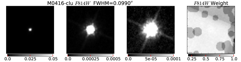
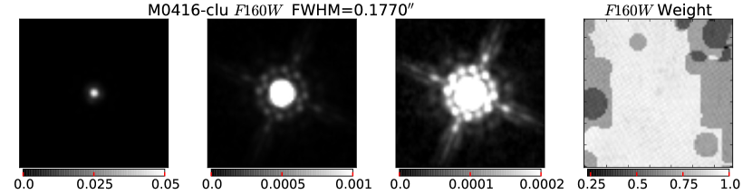
Figure 6.— Point-spread functions (PSFs) for the ACS/$F814W$ band the WFC3/$F160W$ band in the M0416 cluster (all other fields can be found in the Appendix). The construction of the PSFs is described in Section 3.4. For each filter we show three scales (top panels for $F814W$ and bottom for $F160W$ as labeled) to illustrate the structure of the PSF (from left to right: the core, the first Airy ring and the diffraction spikes). The images are normalized to a maximum value of one. The grayscale bars show the scale for each panel. These are different for the ACS and WFC3 as a result of the different FWHMs (listed above the images). We also show the combined weight images for each PSF. The weight is largest in the center and lower at larger radii and not consistent as shown due to masking of neighboring objects (this is the reason for darker circles appearing).

For each field, we create a deep detection image from the bCGs modeled out residual images (see Figure 5, second panels from the right) of the $F814W$, $F105W$, $F125W$, $F140W$ and $F160W$ bands. Before we combine the bands to create the detection image, we perform a separate background subtraction on the five mosaics. This is a separate step, independent from the photometry additional background subtraction (Section 3.2) of each individual band mosaic and is used only for creating the detection image. This background subtraction utilizes a spline interpolation to better smooth and normalize the background to zero improving our detection of sources when the bands are combined. We mask all the residuals from the bCGs and any ICL or contaminant (cosmic ray, bad pixel, etc.) that was missed previously. Then, the images are PSF-matched to the $F160W$ image. We combine these images together to produce a weighted mean mosaic, using the corresponding error images (obtained from the inverse variance maps) to properly weight the images. We divide the weighted mean mosaic by its error image to noise-equalize the weighted mean mosaic. This forms a deep detection image of the central field and larger coverage with the $F814W$ band. Since the variable weight from each band is taken into account using this method, we do not input a weight map to SExtractor during source detection.

As each cluster and parallel field is significantly different, we allow the detection and analysis thresholds to vary slightly from field to field. The detection and analysis thresholds are set in the range of $3-6$ depending on the field’s specific noise properties (same value for both thresholds). We require a minimum area of 4 pixels for detection. The de-blending threshold is set to 32, with a minimum contrast parameter of $5\times 10^{-6}$ for all fields. A Gaussian filter of 4 pixels is used to smooth the images before detection. The detection parameters are chosen as a compromise between de-blending neighboring galaxies and splitting large objects into multiple components (following a similar approach to Skelton et al., 2014). After an initial run, we check the detection image with the sources found to ensure ICL and residuals did not get identified as sources that are not apparent in the individual images but detectable in the deep detection image. For these instances, we mask the detected ICL and residuals and re-run SExtractor with the same parameters as defined previously. This procedure results in the best overall detected sample of sources.

3.4. PSF Matching of the HST Imaging

We PSF-match all the HST ACS and WFC3 mosaics to the $F160W$ mosaic, which has the largest PSF FWHM of the HST filters, before performing aperture photometry using the procedure discussed in Skelton et al. (2014). Below, we summarize and discuss our results for the HST filters.

We create an empirical PSF for each HST mosaic by stacking isolated unsaturated stars. This selection is performed by measuring the ratio of flux within a small aperture to a large aperture to correctly identify appropriate stars, adjusting the criteria as necessary for each band. The number of stars vary for each field and band but the selection results with at least a few stars (3 or more) to tens of stars in each band of the ACS and WFC3 bands. The UVIS bands present more of a challenge as there are not many sources in these bands. However, we are able to make use of at least two or more point-like sources in each band of each field that produces satisfactory results (discussed later in this section and demonstrated by the growth curves in Figure 8). We make postage stamp cut-outs of these stars following the same parameters detailed in Skelton et al. (2014) with a couple of adjustments. Since we do not have dozens of stars to choose from in our fields, we allow for large shifts during the re-centering and normalizing process. Since these are densely packed fields, we do a visual inspection of the PSFs after they are created to check for any contaminants and, if necessary, re-perform the process after additional masking.

In Figure 6, we demonstrate the PSF stamps at three different contrast levels for the ACS/$F814W$ and the WFC3/$F160W$ bands in the M0416 cluster to expose the structure of the PSFs. The structure of the PSFs shown are the core, the first Airy ring ($\sim 0.5$%) and the diffraction spikes ($\sim 0.1$%). Furthermore, the growth curves (that is the fraction of light enclosed as a function of aperture size) for each of the fields are consistent with each other to $<$ 1%, with almost identical curves at this scale (Figure 7). For context, we show the consistency of our growth curves with the encircled energy as a function of aperture provided by the WFC3 handbook (normalized to the radius of $2\farcs 1=35$ pixels).

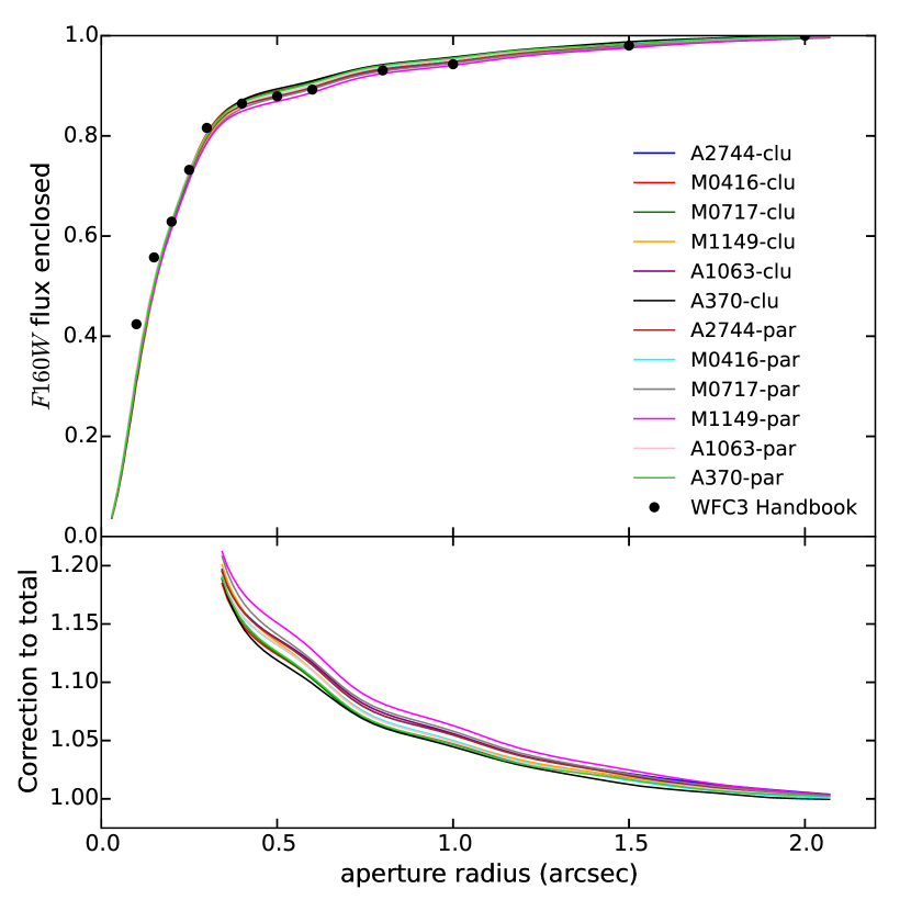
Figure 7.— $F160W$ growth curves. Upper panel: the fraction of light enclosed as a function of radius relative to the total light within $2^{\prime\prime}$, $f(r)/f(2^{\prime\prime})$, from the $F160W$ PSF stamp of each field. The PSFs of the 12 fields are very consistent with each other. The black points show the encircled energy as a function of aperture size, also normalized to $2^{\prime\prime}$, from the WFC3 handbook. The empirical growth curves agree well with the theoretical expectation. Lower panel: the correction to total flux for a point source with a circularized Kron radius equal to the aperture radius on the horizontal axis, derived as the inverse of the growth curves in the upper panel $(f(2^{\prime\prime})/f(r))$. The minimum Kron radius is set to the aperture radius in which we measure photometry, $0\farcs 35$, giving rise to a maximum correction of $\sim$1.19.

As demonstrated by Skelton et al. (2014), we use a deconvolution code that fits a series of Gaussian-weighted Hermite polynomials to the Fourier transform of the stacked stars, to find the kernel that convolves each PSF to match the $F160W$ PSF (developed by I. Labbé). In Figure 8, we demonstrate the ratio of the growth curve in each band to that of the $F160W$ growth curve, before and after the convolution, for the M0416 cluster. The PSF-matching is excellent with an accuracy $<1$ % within a $0\farcs 7$ diameter aperture for all the HST bands and fields (see Appendix).

3.5. HST Photometry

We perform photometry for each HST band with the same method described in Skelton et al. (2014). We summarize the steps below and alterations made to better suit the HFF data. We run SExtractor in dual-mode for each HST band, using the detection images described in Section 3.3 and the PSF-matched HST images described in Section 3.4, adopting an aperture diameter of $0\farcs 7$ as the photometry aperture flux for all HST bands. We determine the total flux from the $F160W$ band, where the $F160W$ band has coverage, and the $F814W$ band otherwise (a few sources use the other detection bands depending on band coverage, i.e. “bandtotal” column in the catalogs). We correct the SExtractor AUTO flux using the inverse of the fraction of light within a circular aperture that is equivalent to the Kron aperture determined from our growth curves. For sources with AUTO flux radii smaller then the photometry aperture radius, we take the photometry aperture flux multiplied by the corresponding correction factor to be the total flux.

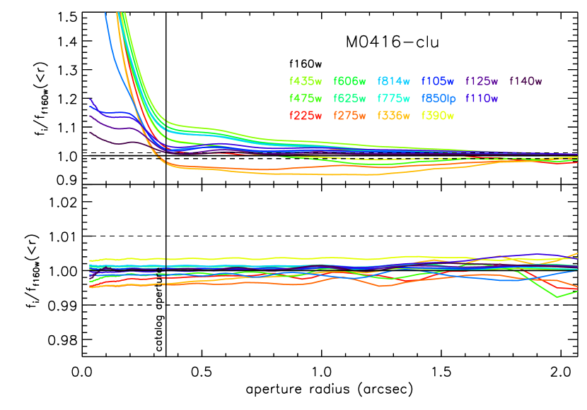
Figure 8.— Growth curves showing the fraction of light enclosed as a function of radius for each HST filter relative to the $F160W$ growth curve in the M0416 cluster (all other fields can be found in the Appendix). The upper and lower panels show the growth curves before and after convolution to match the $F160W$ PSF, respectively. Note the change in scale between the upper and lower panels. The dashed line in each panel represents a 1% difference from the $F160W$ PSF. After PSF-matching, the resulting growth curves in all bands are consistent with the $F160W$ PSF to well within 1%.

We estimate the uncertainty on the total flux using empty apertures of the background noise in increasing size within the noise-equalized images for each band. For each aperture size, we measure the flux in more than 2000 apertures placed at random positions across the image excluding apertures that overlap with sources in the detection segmentation map. We find including more apertures is not necessary for accurate error analysis and became difficult at larger radii for certain bands (e.g. the WFC3 bands).

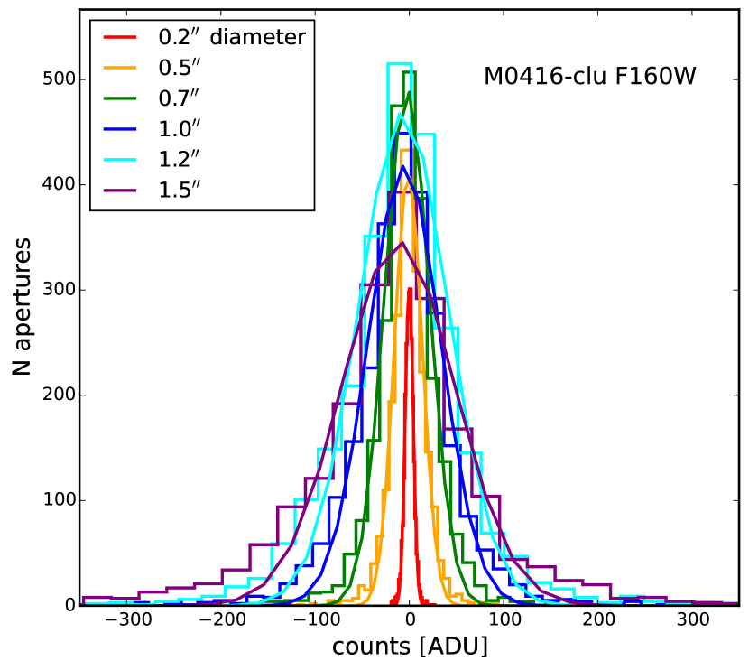
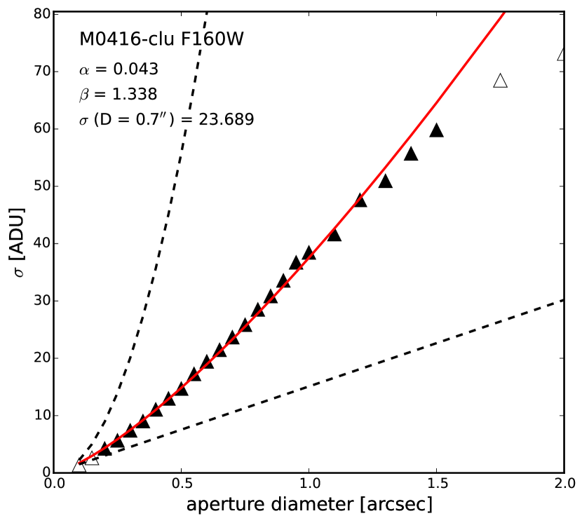
Figure 9.— Summed counts of different apertures sizes for empty regions sampling the image (left panel) and the scaling of the noise as a function of the aperture size (right panel) for the M0416 $F160W$ cluster image (all other fields can be found in the Appendix). The histograms are color-coded by aperture size and given in the figure. The measured $\sigma$ are shown by the triangles. The solid line shows the power-law fit to the data, with the fit parameters given in the figure. The dashed lines show the linear ($\propto N$) and $N^{2}$ scalings, which correspond to no correlation and perfect correlation between the pixels, respectively. The $\sigma$ listed is for the photometry aperture size (units of ADU).

Figure 9 (left panel) demonstrates our results for the M0416 cluster for each aperture size well-described by a Gaussian, with increasing width as aperture size increases. The measured deviation is described as a function of aperture size in the M0416 cluster noise-equalized $F160W$ image by fitting a power law to the trend. We fit a power-law (solid line in Figure 9, right panel) of the form

$$\sigma=\sigma(D=0\farcs 7)\alpha N^{\beta},$$ (1)

where $\sigma$(D$=0\farcs 7$) is the standard deviation of the background pixels at the photometry aperture size (in ADU), $\alpha$ is the normalization and $1<\beta<2$ (dashed lines in the figure of $\beta=1$ and $\beta=2$ scalings). The values for each field are given in Table 4. We estimate the uncertainty from this analysis by dividing the median value from the square root of the weight at the position of the object within the circularized Kron radius (see Skelton et al., 2014, for more details). This error term is added in quadrature to the Poisson error to calculate the final uncertainty of each source in the catalog.

3.6. Low Resolution Photometry

The significant differences between the HST data and, the ground-based $K_{S}$ and Spitzer/IRAC data image quality must be quantified, specifically the large differences in the PSF sizes of the Spitzer data. This will allow for accurate information to be obtained without degrading the HST images. We use MOPHONGO, a code developed by one of us (I. Labbé), to perform photometry of these longer wavelength bands ($K_{S}$ and Spitzer/IRAC), as described in Labbé et al. (2006); Wuyts et al. (2007); Whitaker et al. (2011) following the steps of Skelton et al. (2014) (see their Section 3.5 for detailed description).

Table 4Power-law Parameters for Empty Aperture Errors

Field	$\alpha$	$\beta$
A2744-clu	0.027	1.543
A2744-par	0.038	1.401
M0416-clu	0.043	1.338
M0416-par	0.038	1.395
M0717-clu	0.030	1.506
M0717-par	0.039	1.400
M1149-clu	0.032	1.463
M1149-par	0.042	1.354
A1063-clu	0.028	1.526
A1063-par	0.035	1.432
A370-clu	0.036	1.416
A370-par	0.033	1.457

Note. — These parameters are for the $F160W$ band.

Briefly, the code uses a high-resolution image as a prior to estimate the contributions from neighboring blended sources in the lower resolution image. We use the detection image as the high-resolution prior. A map is created to cross-correlate the source positions in the two images. Then the position-dependent convolution kernel that maps the higher resolution PSF to the lower resolution PSF is determined by fitting a number of point sources across each image. The high resolution image is convolved with the local kernel to obtain a model of the low resolution image, with the flux normalization of individual sources as a free parameter. We perform photometry on the original low-resolution image using an aperture appropriate for the size of the PSF (i.e., D$=0\farcs 7$ and D=3” for the $K_{S}$ and IRAC bands, respectively), with a correction applied for contamination from neighboring sources around each object as determined from the model. Further flux corrections are applied to account for flux that falls outside of the aperture from the larger PSF.

3.7. Flux Corrections

We correct for Galactic extinction using the values given by the NASA Extragalactic Database extinction law calculator at the center of each field, again using the same method presented in Skelton et al. (2014). However, we do not interpolate over the dataset for the filters in our catalogs but explicitly calculate the extinction for each field and filter. The Galactic extinction values applied to our dataset are given in Table 5 for each field and filter. We follow the rest of the flux corrections steps by Skelton et al. (2014) that are summarized briefly in the following paragraph.

Table 5Galactic Extinctions for the Hubble Frontier Fields Filters

Filter	A2744	M0416	M0717	M1149	A1063	A370
	clu / par	clu / par	clu / par	clu / par	clu / par	clu / par
UVIS $F225W$	…	0.286 / …	0.535 / …	0.160 / …	0.086 / …	…
$F275W$	0.072 / …	0.225 / …	0.420 / …	0.126 / …	0.067 / …	0.178 / …
$F336W$	0.058 / …	0.182 / …	0.341 / …	0.102 / …	0.055 / …	0.144 / …
$F390W$	…	0.160 / …	0.298 / …	0.089 / …	0.048 / …	…
ACS $F435W$	0.047 / 0.044	0.148 / 0.152	0.276 / 0.275	0.083 / 0.086	0.044 / 0.044	0.117 / 0.110
$F475W$	…	0.134 / …	0.250 / …	0.075 / …	0.040 / …	0.106 / …
$F555W$	…	…	0.214 / …	0.064 / …	…	…
$F606W$	0.032 / 0.030	0.101 / 0.104	0.189 / 0.116	0.057 / 0.059	0.030 / 0.030	0.080 / 0.076
$F625W$	…	0.091 / …	0.170 / …	0.051 / …	0.027 / …	0.072 / …
$F775W$	…	0.067 / 0.069	0.125 / …	0.037 / …	0.020 / …	…
$F814W$	0.020 / 0.019	0.062 / 0.064	0.117 / 0.116	0.035 / 0.036	0.019 / 0.019	0.049 / 0.047
$F850LP$	…	0.051 / 0.052	0.095 / …	0.028 / …	0.015 / …	…
WFC3 $F105W$	0.013 / 0.012	0.040 / 0.041	0.074 / 0.074	0.022 / 0.023	0.012 / 0.012	0.031 / 0.030
$F110W$	…	0.036 / …	0.067 / …	0.020 / …	0.011 / …	0.029 / …
$F125W$	0.010 / 0.009	0.030 / 0.031	0.056 / 0.055	0.017 / 0.017	0.009 / 0.009	0.024 / 0.022
$F140W$	0.008 / 0.008	0.025 / 0.026	0.047 / 0.047	0.014 / 0.015	0.008 / 0.007	0.020 / 0.019
$F160W$	0.007 / 0.006	0.021 / 0.022	0.039 / 0.039	0.012 / 0.012	0.006 / 0.006	0.017 / 0.016
$K_{S}$   $2.2\micron$	0.004 / 0.004	0.013 / 0.013	0.024 / 0.024	0.007 / 0.007	0.004 / 0.004	0.010 / 0.009
IRAC $3.6\micron$	0.002 / 0.002	0.007 / 0.008	0.014 / 0.014	0.004 / 0.004	0.002 / 0.002	0.006 / 0.005
$4.5\micron$	0.002 / 0.002	0.006 / 0.006	0.011 / 0.011	0.003 / 0.004	0.002 / 0.002	0.005 / 0.005
$5.8\micron$	0.002 / …	…	…	…	0.002 / …	0.004 / …
$8.0\micron$	0.002 / …	…	…	…	0.001 / …	0.004 / …

Note. — Galactic extinction values for the available filters for each field (see Section 3.7 for more details). The cluster and parallel fields are designated by clu / par for the HFF. We denote filters where no imaging data is available with ellipses (…). All values are in AB magnitude.

The fluxes provided in the catalogs are total fluxes. We correct the photometry aperture flux measured in each HST band to a total flux by multiplying the ratio of the $F160W$ total flux to the $F160W$ flux measured in the 0$\farcs$7 aperture. The total flux for the $F160W$ reference band is calculated from the SExtractor’s AUTO flux and using the circularized Kron radius in combination with the $F160W$ growth curve (see Section 3.5). However, the $F814W$ (in a few cases, $F105W$, $F125W$, or $F140W$) is used instead of the $F160W$, when the $F160W$ has no coverage. We indicate this with “bandtotal” in the catalogs (see Table 6 and Section 3.11). The photometry aperture errors are converted to a total error by multiplying by the same correction as the fluxes. We perform the same process for the $K_{S}$ and IRAC bands but for apertures of $0\farcs 7$ and 3″, respectively.

3.8. Point Source Classification

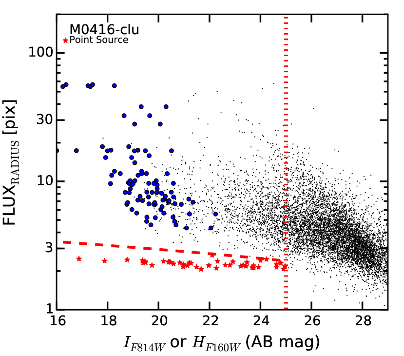
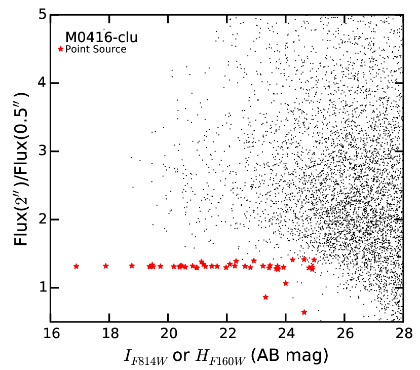
Figure 10.— The Left panel demonstrates SExtractor’s FLUX_RADIUS against total $H_{F160W}$ magnitude when available or $I_{F814W}$ magnitude otherwise for the M0416 cluster (all other fields can be found in the Appendix). Objects classified as point sources in the catalog are shown with red stars, galaxies and uncertain classifications as black points, modeled out bCGs as blue circles. The Right panel demonstrates an alternate method for selecting point sources using the ratio of fluxes in a large and small apertures. The tightness of the stellar sequence in this ratio at brighter magnitudes ($H_{F160W}\mathrel{\hbox{\hbox to0.0pt{\lower 2.36806pt\hbox{$\sim$}\hss} \kern-3.00003pt\raise 1.72218pt\hbox{$<$}}}24$ mag) allows for a more stringent classification, but the separation becomes less clear than the flux radius selection at fainter magnitudes. In general, the two methods yield similar results for each field.

Compact or unresolved sources (i.e. point sources) have a tight correlation in size and magnitude, with fairly constant, small sizes as a function of magnitude. We demonstrate this trend in Figure 10 that shows the SExtractor FLUX_RADIUS against total $H_{F160W}$ magnitude when available or the $I_{F814W}$ magnitude otherwise, for the M0416 cluster (left panel).

Table 6Catalog Columns

Column Name	Description
id	Unique identifier for HFF-DeepSpace
x	X centroid in image coordinates
y	Y centroid in image coordinates
ra	RA J2000 (degrees)
dec	Dec J2000 (degrees)
z_spec	Spectroscopic redshift, when available
flags_band	SExtractor extraction flags (SExtractor FLAGS parameter)
class_star_band	Stellarity index (SExtractor CLASS_STAR parameter)
flux_radius	Circular aperture radius enclosing half the total flux (SExtractor FLUX_RADIUS parameter, pixels)
star_flag	Point source = 1, extended source = 0, uncertain source = 2 (source $\geq$ 25 mag)
bandtotal	Either “$F160W$”, “$F140W$”, “$F125W$”, “$F105W$”, “$F814W$”, “bcg” or “none”; band used to derive total fluxes
f_band	Total flux for each band (zero point = 25)
e_band	$1\sigma$ error for each band (zero point = 25)
w_band	Weight relative to maximum exposure within image band (see Section 3.11)
flag_band	Identifies possibly problematic sources for each band (see Section 3.9)
use_band	Identifies possibly problematic photometry for low resolution bands (see Section 3.9)
REFspecz	Literature reference for spectroscopic redshift
theta_J2000	Position angle of the major axis (counter-clockwise, measured from East)
kron_radius	SExtractor KRON_RADIUS (pixels)
a_image	Semi-major axis (SExtractor A_IMAGE, pixels)
b_image	Semi-minor axis (SExtractor B_IMAGE, pixels)
use_phot	Flag indicating source is likely to be a galaxy with reliable photometry (see Section 3.10)
mwext_band	Applied Milky Way extinction correction for each band (see Table 5)
zpcorr_band	Applied zero point correction for each band (see Table 10)

Point sources can be separated cleanly from extended sources down to $H_{F160W}$ or $I_{F814W}\sim 25$ mag. We provide a point source flag in the catalog based on the criteria here, as measured on the $F160W$ images when available and $F814W$ otherwise (a few sources utilize the other detection bands, i.e. the $F105W$, $F125W$ and $F140W$; this is based on their “bandtotal” band, refer to Table 6). Objects are classified as point sources (star_flag = 1) if they have $\mathrm{FLUX\_RADIUS}<-\,0.11\,H_{F160W}+5.15$, where $H_{F160W}$ is the total magnitude of the band used for total flux (i.e. “bandtotal”). We also perform visual inspection on the images to determine if any stars are missed or if any sources should be excluded from the above selection. Due to the small effective areas of these fields with consequently low number of stars, this was a useful task to perform. These sources are shown with red stars in Figure 10. Sources fainter than 25 mag (dotted red line in figure) can not be identified accurately as point sources (unless by visual inspection) and are assigned star_flag = 2. All other objects are classified as extended, with star_flag = 0.

Another method for classifying point sources is the ratio of fluxes in large ($2\arcsec$) and small ($0\farcs 5$) apertures versus magnitude that provides a similar tight sequence for $I_{F814W}$ or $H_{F160W}\lesssim 24$ mag (right panel of Figure 10). Both sequences prove to be useful diagnostics of the image quality, and demonstrate the dearth of stars in these small effective area fields.

3.9. Flags

To better distinguish the quality of the photometry for the sources in the catalogs, we provide flags that allow straightforward selection of sources that have photometry of reasonably uniform quality. For each photometric band, this flag_band is set to 0 (i.e. “OK”) if none of the following criteria are met (e.g. flag_F160W = 0):

1. The photometry aperture overlaps with a masked region: flag set to flag_band = 1.

2. The AUTO aperture from SExtractor overlaps with a masked region: flag_band = 2.

3. Both the photometry and AUTO apertures overlap with a masked region: flag_band = 3. This occurs mostly for faint and extremely extended sources (e.g. gravitationally lensed arcs).

4. The source is a selected bCG for modeling (see Section 3.1.1) that could not be modeled out: flag_band = 4. This primarily applies to the UV bands as bCGs became to faint for modeling.

5. The weight value is $\leq$ 0 for any pixels associated with the source in the segmentation map: flag_band = -1.

We mask regions that are influenced significantly by any of the following: bright stars that cause halos and large diffractions spikes, residual of a modeled out bCG, satellite trails, cosmic rays, and pixels that have weight values $\leq$ 0. For bad pixels not caught by cosmic ray detection and the weight images, the masking is done manually through visual inspection of each science image for the HST photometric bands before and after the bCG modeling and sky subtraction steps (see Section 3.1).

For the non-HST bands, the $K_{S}$ and Spitzer/IRAC bands, we use a simplified ‘use’ flag assignment due to the differences in the methods performed for photometry (i.e. MOPHONGO instead of SExtractor). For each photometric band of the $K_{S}$ and Spitzer/IRAC, this ‘use_band’ flag is set to 1 (i.e. “GOOD”) if none of the following criteria are met (e.g. use_CH1 = 1).

1. If any of the flux, error or weight $\leq$ 0 and/or NaN/Inf values: flag set to use_band $=0$ (i.e. “BAD”).

2. The source is a selected bCG for modeling (see Section 3.1.1): flag set to use_band = 2.

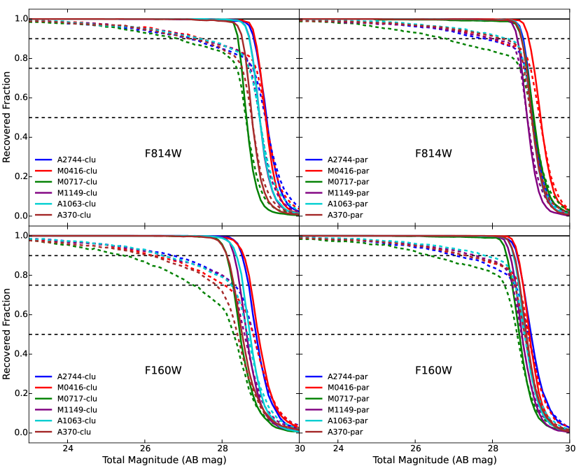
Figure 11.— Completeness fraction as a function of total magnitude for the deep region (reg1) in each field. We show no-overlap criterion (solid lines) and “allow” overlap criterion (dashed lines) for the $I_{F814W}$ (top panels) and $H_{F160W}$ (bottom panels) bands (see Section 3.12). In both cases (no-overlap and “allow” overlap), the 75% completeness fraction agrees within one magnitude for each field, respectively, in both bands.

3.10. “use_phot”

We introduce use_phot following Skelton et al. (2014) that selects “OK” sources in a consistent way. By selecting sources with use_phot = 1, this excludes stars (i.e. star_flag = 0 or 2 are “OK”), sources close to a bright star, S/N $\leq 3$ from the photometry aperture in the ‘bandtotal’ band (see Section 3.11), “non-catastrophic” photometric redshift fit ($\chi_{\mathrm{p}}<1000$, see Section 5.2) and ”non-catastrophic” stellar population fit (log$(M)>0$, see Section 5.4).

The use_phot flag selects approximately 80% of all objects in the catalogs. The flag is not very restrictive and is meant as a guide to inform the user of possibly problematic sources in the catalogs. In most science cases, further cuts are required (particularly on magnitude, number of available photometric bands, and/or a stricter S/N ratio). For studies of large samples, the ‘use_phot’ flag should be sufficiently reliable when combined with a magnitude criterion. For an individual galaxy or small sample, we caution the reader to inspect the quality of the photometry for each source beyond the selection criteria.

3.11. Catalog Format

We provide a full photometric catalog for each of the six HFF clusters and associated parallels. The catalogs contain total flux measurements and basic galaxy properties for 81315 objects in total - (9390, 6240), (7431, 7771), (6370, 5776), (6868, 5802), (7611, 5574) and (6795, 5687) for A2744, M0416, M0717, M1149, A1063 and A370, clusters and parallels, respectively.

A description of the columns in each photometric catalog is given in Table 6. All fluxes are normalized to an AB zero point of 25, such that

$$\mathrm{mag}_{AB}=-2.5\times\log_{10}(F)+25.$$ (2)

The total fluxes and $1\sigma$ errors for every band listed in Table 5 are given in the photometric catalogs. The structural parameters from SExtractor and the corrections to total fluxes are derived from the $F160W$ image, where there is $F160W$ coverage and the other detection bands otherwise. The ‘bandtotal’ column indicates which image was used to derive total fluxes.

We provide a weight column for each band to indicate the relative weight for each object compared to the maximum weight for that filter. In practice, the weight is calculated as the ratio of the weight at each object’s position to the 95^th percentile of the weight map. We take the median weight value from a $7\times 7$ grid of pixels around the central pixel of the source and divide by the 95^th percentile pixel weight value of the image from the positive non-zero weights (i.e. no masked regions are used). We use the 95^th percentile weight, as opposed to the maximum, to avoid extreme values affecting the maximum weight. Objects with weights greater than the 95^th percentile weight have a value of 1 in the weight column.

3.12. Completeness

Table 7Completeness Fraction as a Function of $F814W$ Magnitude

		No$-$Overlap			“Allow”$-$Overlap
Field	90%	75%	50%	90%	75%	50%
	reg1 (reg2) [reg3]	reg1 (reg2) [reg3]	reg1 (reg2) [reg3]	reg1 (reg2) [reg3]	reg1 (reg2) [reg3]	reg1 (reg2) [reg3]
A2744-clu	28.8 (28.5) [27.4]	29.0 (28.7) [27.6]	29.2 (28.9) [27.7]	27.2 (27.8) [27.0]	28.8 (28.6) [27.5]	29.1 (28.9) [27.7]
A2744-par	28.8 (28.5) [$\dots$]	28.9 (28.6) [$\dots$]	29.1 (28.8) [$\dots$]	27.8 (27.9) [$\dots$]	28.8 (28.5) [$\dots$]	29.1 (28.7) [$\dots$]
M0416-clu	28.9 (28.5) [26.3]	29.0 (28.6) [26.5]	29.1 (28.8) [26.7]	27.5 (27.4) [26.3]	28.9 (28.5) [26.4]	29.1 (28.8) [26.7]
M0416-par	28.9 (28.7) [$\dots$]	29.1 (28.8) [$\dots$]	29.2 (29.0) [$\dots$]	28.0 (28.4) [$\dots$]	29.0 (28.7) [$\dots$]	29.2 (29.0) [$\dots$]
M0717-clu	28.4 (28.1) [26.3]	28.5 (28.2) [26.6]	28.6 (28.3) [26.8]	26.9 (27.2) [26.1]	28.4 (28.1) [26.6]	28.6 (28.3) [26.8]
M0717-par	28.8 (28.4) [26.8]	28.9 (28.5) [27.0]	29.1 (28.7) [27.2]	26.8 (27.4) [26.8]	28.7 (28.4) [27.0]	29.0 (28.6) [27.2]
M1149-clu	28.7 (28.4) [$\dots$]	28.8 (28.5) [$\dots$]	29.0 (28.7) [$\dots$]	27.4 (27.7) [$\dots$]	28.7 (28.4) [$\dots$]	29.0 (28.6) [$\dots$]
M1149-par	28.6 (28.3) [26.1]	28.8 (28.4) [26.3]	28.9 (28.6) [26.5]	28.0 (27.4) [26.1]	28.7 (28.3) [26.3]	28.9 (28.6) [26.5]
M0717-clu	28.7 (28.4) [26.4]	28.8 (28.5) [26.8]	29.0 (28.7) [27.0]	27.4 (27.4) [26.4]	28.7 (28.5) [26.8]	29.0 (28.7) [27.0]
M0717-par	28.8 (28.4) [$\dots$]	28.9 (28.6) [$\dots$]	29.0 (28.7) [$\dots$]	28.4 (28.1) [$\dots$]	28.8 (28.5) [$\dots$]	29.0 (28.7) [$\dots$]
A370-clu	28.5 (28.2) [26.7]	28.6 (28.3) [27.2]	28.8 (28.4) [27.5]	27.1 (27.2) [26.6]	28.5 (28.2) [27.1]	28.8 (28.4) [27.5]
A370-par	28.8 (28.4) [$\dots$]	28.9 (28.6) [$\dots$]	29.0 (28.8) [$\dots$]	28.3 (27.6) [$\dots$]	28.8 (28.5) [$\dots$]	29.0 (28.7) [$\dots$]

Note. — Reg1 is the deepest region with Reg3 being the shallowest region for each field. When Reg3 is too small for meaningful calculations of the completeness, no completeness value is given ($\dots$). All values are in AB magnitude.

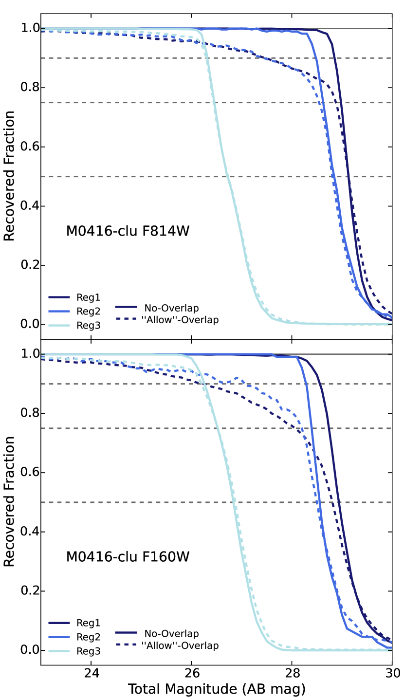
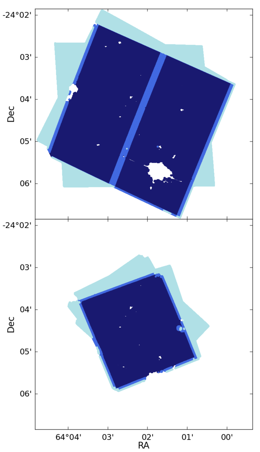
Figure 12.— We demonstrate the recovered completeness fraction of each region in the M0416 cluster for both the no-overlap (solid lines) and “allow” overlap (dashed lines) criteria (all other fields can be found in the Appendix, see Section 3.12 for details). The Top panels are the $F814W$ band and the Bottom panels of the $F160W$ band, where the areas for each region (Right panels) are shaded by region (reg1 is midnight blue; reg2 is royal blue; reg3 is powder blue) corresponding to the line colors (Left panels).

Table 8Completeness Fraction as a Function of $F160W$ Magnitude

		No$-$Overlap			“Allow”$-$Overlap
Field	90%	75%	50%	90%	75%	50%
	reg1 (reg2) [reg3]	reg1 (reg2) [reg3]	reg1 (reg2) [reg3]	reg1 (reg2) [reg3]	reg1 (reg2) [reg3]	reg1 (reg2) [reg3]
A2744-clu	28.5 (28.2) [26.5]	28.7 (28.3) [26.6]	28.9 (28.5) [26.8]	26.7 (26.4) [26.3]	28.3 (28.2) [26.5]	28.8 (28.5) [26.7]
A2744-par	28.6 (28.2) [$\dots$]	28.8 (28.3) [$\dots$]	29.0 (28.5) [$\dots$]	27.1 (26.5) [$\dots$]	28.6 (28.3) [$\dots$]	28.9 (28.5) [$\dots$]
M0416-clu	28.6 (28.3) [26.3]	28.7 (28.4) [26.5]	28.9 (28.6) [26.8]	26.2 (27.1) [26.2]	28.1 (28.2) [26.5]	28.8 (28.5) [26.9]
M0416-par	28.7 (28.3) [$\dots$]	28.8 (28.4) [$\dots$]	29.0 (28.6) [$\dots$]	27.3 (27.2) [$\dots$]	28.7 (28.4) [$\dots$]	28.9 (28.6) [$\dots$]
M0717-clu	28.1 (27.8) [26.3]	28.3 (27.9) [26.5]	28.5 (28.1) [26.7]	25.5 (26.1) [26.2]	27.3 (27.6) [26.4]	28.3 (28.0) [26.7]
M0717-par	28.4 (27.9) [26.7]	28.5 (28.1) [26.8]	28.7 (28.3) [27.0]	26.4 (24.9) [26.6]	28.3 (27.4) [26.8]	28.6 (28.2) [27.0]
M1149-clu	28.3 (28.0) [26.1]	28.5 (28.1) [26.4]	28.6 (28.3) [26.9]	26.5 (26.4) [25.9]	28.2 (27.9) [26.4]	28.6 (28.2) [26.9]
M1149-par	28.5 (28.0) [27.0]	28.6 (28.2) [27.2]	28.8 (28.3) [27.4]	27.6 (27.2) [26.8]	28.5 (28.1) [27.1]	28.8 (28.4) [27.3]
A1063-clu	28.4 (28.0) [26.5]	28.5 (28.1) [26.6]	28.7 (28.3) [26.8]	26.5 (26.5) [26.4]	28.2 (27.9) [26.6]	28.7 (28.3) [26.8]
A1063-par	28.5 (28.2) [26.8]	28.7 (28.3) [27.0]	28.8 (28.5) [27.1]	27.8 (28.0) [26.7]	28.6 (28.3) [26.9]	28.8 (28.5) [27.1]
A370-clu	28.1 (27.8) [26.7]	28.3 (27.9) [26.9]	28.5 (28.1) [27.1]	26.1 (26.4) [26.5]	27.8 (27.7) [26.9]	28.4 (28.1) [27.1]
A370-par	28.6 (28.1) [$\dots$]	28.7 (28.3) [$\dots$]	28.9 (28.5) [$\dots$]	27.3 (28.0) [$\dots$]	28.6 (28.3) [$\dots$]	28.8 (28.5) [$\dots$]

Note. — Reg1 is the deepest region with Reg3 being the shallowest region for each field. When Reg3 is too small for meaningful calculations of the completeness, no completeness value is given ($\dots$). All values are in AB magnitude.

The depth of the images varies from field to field and towards the edges of some fields (e.g. A2744 cluster). As a result, the completeness will depend on position, as well as different morphologies, magnitudes and sizes. Here, we describe the completeness for point sources in the HFF cluster and parallel fields. We measure the recovered fraction for the $H_{F160W}$ and $I_{F814W}$ bands of each field. We do this by inserting fake stars, generated from the convolved PSF at random positions in the field, using the weight and segmentation maps to exclude pixels when determining random pixel locations. First, we do not allow the fake stars to overlap with detected sources in the field. Then, we allow the fake stars to overlap, to calculate the effect of blending in crowded fields. We sample the recovered fraction of fake stars at magnitude intervals of 0.1 for about 2000 fake stars in each field and band.

Furthermore, we do this by dividing the images into deep and shallow regions (shallow regions are generally near the edges of the mosaics) for each field and band. The following criteria are used to separate the deep region from the shallower regions:

$$\begin{split}reg1:&wht\geq 0.6\times wht(95^{th})\\ reg2:&0.25\times wht(95^{th})\leq wht<0.6\times wht(95^{th})\\ reg3:&wht<0.25\times wht(95^{th})\\ &Area(reg3)>0.05\times Area(total)\end{split}$$ (3)

where $wht(95^{th})$ is the 95th percentile of the weight distribution, and Area(total) is the total area of all three regions.

We measure the completeness for the deeper regions (reg1 and reg2) in each field and band, but only measure the shallowest region (reg3) if the Area requirement of equation 3 is met. We make a single-band detection image for each region in the same way as the detection image discussed previously (i.e. weighted_mean / error image) and apply the same SExtractor parameters (see Section 3.3). However, we do lower the detection and analysis thresholds to account for the shallower depth of the single-band detection image (range of $2.5-4.0$ for $F814W$ and $1.1-1.4$ for $F160W$). We run SExtractor in dual mode with the final residual image for each field and band as the measurement image ($F160W$ and $F814W$, see Figure 5).

In Figure 11, we demonstrate the completeness fraction as a function of total magnitude for the deep region (reg1) in each field. Tables 7 and 8 list the 90%, 75% and 50% completeness levels for each field of the no-overlap and “allow” overlap criteria for the $F814W$ and $F160W$ bands, respectively. The comparison between the no-overlap and “allow” overlap completeness levels shows that very deep fields like the Hubble Frontier Fields, hence crowded fields, blending significantly affects the completeness.

Figure 12 demonstrates the completeness fraction as a function of magnitude for each region in the M0416 cluster. The completeness fraction is measured for both the $F814W$ (top panels) and $F160W$ (bottom panels) bands, where the areas for each region (right panels) are shaded by region corresponding to the line colors (reg1 is midnight blue; reg2 is royal blue; reg3 is powder blue). Furthermore, we show both the no-overlap (solid lines) and “allow” overlap (dashed lines) recovered fractions for each band (left panels). In most cases, the deeper regions (reg1 and reg2) have similar recovered completeness fractions, where the shallowest region (reg3) differs significantly by about 2 magnitudes regardless of allowing overlap or no-overlap (see Tables 7 and 8 for specific values of each field and band).

3.13. Number Counts

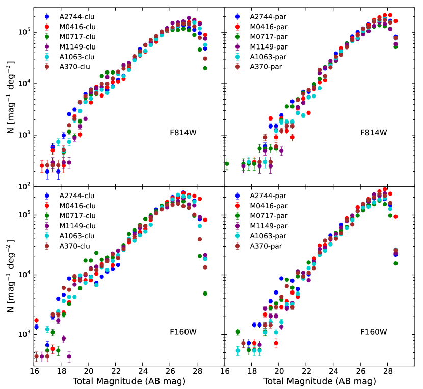
Figure 13.— Number counts per unit area. The left panels show the number counts of galaxies (use_phot = 1) per square degree in each of the six cluster fields as a function of $I_{F814W}$ or $H_{F160W}$ total magnitude (labeled in each panel), with no correction for incompleteness. In the right panels, we repeat this for the six parallel fields. The error bars on all the data points represent Poisson errors. Lensing magnification corrections have not been applied.

We determine the effective survey area of each of the six cluster and six parallel fields using the detection image of each field with the following steps. For each of the detection band images, we create a map of the number of detection bands contributing to each pixel. We do not include regions masked out during photometry of each detection band as described in Section 3.9. Then, the science area for each field is calculated by adding up the number of unmasked pixels within the detection band area of our catalogs. We follow this same procedure for single band effective areas, specifically the $I_{F814W}$ and $H_{F160W}$ bands.

The number density of galaxies (satisfying our “use_phot” flag criteria in the HFF), as a function of the $H_{F160W}$ magnitude, is shown in Figure 13 (bottom panels). The bottom left panel shows the number counts for each of the six cluster fields, while the bottom right panel repeats this for the six parallel fields. The error bars represent Poisson errors in both panels. Considering the very small field of view of each pointing, the number counts are fairly consistent across the six cluster and six parallel fields. Figure 13 (top panels) show the number density of galaxies as a function of $I_{F814W}$ magnitude. For both the $H_{F160W}$ and $I_{F814W}$ number density of galaxies figures, we use their respective effective areas given in Table 1.

3.14. Photometry of Close Pairs

We do extensive work to model out the light from the bCGs and ICL and ensure the quality of the final science images but this does not extend to remaining close pair sources. To this end, we caution the reader that the photometry of sources may not account for systematic offsets from nearby sources in the formal uncertainties given in the catalogs.

The ground-based $K_{S}$ band and IRAC photometry is performed after subtracting a model for neighboring sources (see Section 3.6), but the space-based photometry is performed directly on PSF-matched data without explicitly accounting for the flux of nearby sources. SExtractor does attempt to mask and correct the aperture fluxes symmetrically for regions affected by overlapping sources (with the MASK_TYPE parameter set to CORRECT). As described in Section 3.5, the photometry aperture has a diameter of $0\farcs 7$.

We estimate the fraction of potentially affected sources in the catalogs by determining the number of sources with a distance smaller than the photometry aperture (i.e., with overlapping photometric apertures $<0\farcs 7$ and use_phot = 1). These fractions range from 11.3% to 15.2% in the six cluster fields, with an average of 13.2%. We repeat this for the six parallel fields and find similar amounts of close pairs with fractions ranging from 10.9% to 13.6% (average of 12.1%). If we assume that only the faintest overlapping source of the pair ($H_{F160W}$ ¿ 25 mag) is affected, we determine that 5.0% to 8.6% (average of 6.4%) of sources may have problematic HST photometry due to contamination of a nearby source for both the clusters and parallel fields.

4. Quality and Consistency Tests

Here we assess the quality of our photometric catalogs. We test whether the colors and uncertainties are reasonable and if there are offsets between the fields.

4.1. Colors

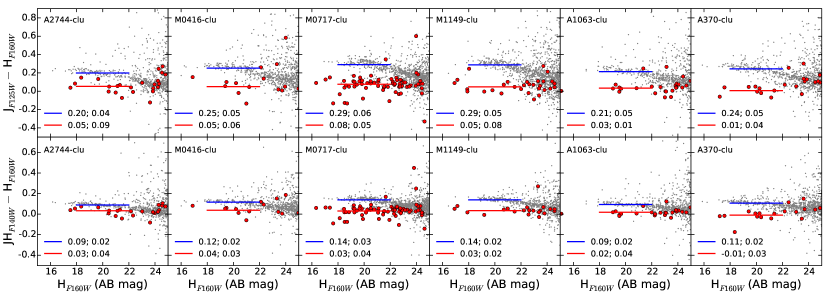
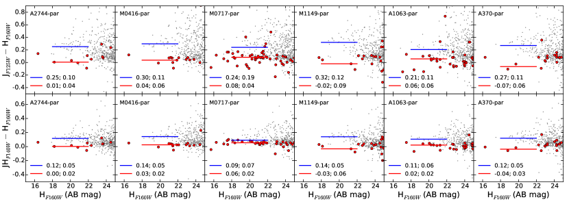
Figure 14.— $J_{F125W}-$ $H_{F160W}$ and $JH_{F140W}-$ $H_{F160W}$ colors versus $H_{F160W}$ magnitude for each of the twelve fields (clusters top half of figure and parallels bottom half of figure). Point sources (star_flag = 1) are shown in red and extended sources (use_phot = 1) in gray. The medians and their scatter ($\sigma_{\mathrm{MAD}}$) for point sources and extended sources in the range $18<H_{F160W}<22$ are labeled and shown by the red and blue lines, respectively for both clusters and parallels (see Section 4.1 for discussion).

In order to determine if there are offsets between the fields, we look at $J-H$ colors in each field for stars (flag_star = 1) and galaxies (use_phot = 1), specifically the median observed colors of the two groups assuming they do not have a dependence on field. Figure 14 (top panels) demonstrates this comparison for the clusters. We repeat this for the parallels (Figure 14, bottom panels). For each panel, the red and blue lines show the median color in the magnitude range $18<H_{F160W}<22$ for stars and galaxies, respectively, with the median and scatter from the median absolute deviation (MAD, Beers et al., 1990, $\sigma_{\mathrm{MAD}}$) values listed in each panel, respectively. The top row, for each set of panels, shows the relation between $J_{F125W}-H_{F160W}$ color and $H_{F160W}$ magnitude in each cluster and parallel field. The bottom row, for each set of panels, shows the relation between $JH_{F140W}-H_{F160W}$ color and magnitude. The scatter seen for the stars and galaxies is expected due to the fact that not all stars and galaxies have similar colors.

We find that the median WFC3 colors show very little field dependence for the clusters and parallels, when considering the expected scatter of the data and in the case of the stars having low statistics for some of the fields (e.g. M1149 and A370 parallels). Although, the median colors of the galaxies for the clusters do vary slightly due to the different redshifts. The median galaxy colors are reddest in M0717 and M1149 clusters, which are the highest redshift. The field-to-field variation ($\sigma_{\mathrm{MAD}}$) in the median $J_{F125W}-H_{F160W}$ color is $\sim 0.037$ mag for stars and $\sim 0.059$ mag for galaxies. The $JH_{F140W}-H_{F160W}$ colors show even less variation between fields for the stars and galaxies than the $J_{F125W}-H_{F160W}$ colors: the field-to-field variation ($\sigma_{\mathrm{MAD}}$) in the median color of stars (galaxies) is $\sim 0.015$ ($\sim 0.030$) mag.

4.2. Total Fluxes

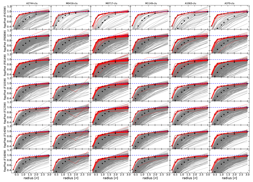
Figure 15.— Ratio of aperture flux to total flux given in the catalogs as a function of aperture radius in each HFF cluster and HFF band. We select sources with high signal-to-noise ratios (S/N ¿ 50) for better comparison. In each case a few hundred extended sources were chosen randomly from the catalog (except for the $F435W$ band) with the requirement that each source satisfy use_phot = 1 in addition to the S/N cut. Point sources (star_flag = 1) are shown in red and extended sources in gray. The median values for point sources and extended sources are shown by the large stars and filled circles, respectively. We find good agreement between the derived total fluxes and the direct measurements of flux in $3^{\prime\prime}$ apertures, to within a percent for point sources. Furthermore, the measurements are consistent across all clusters with few spurious sources.

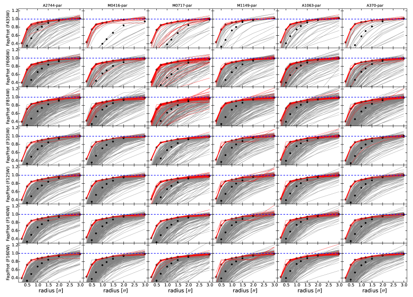
Figure 16.— Same as Figure 15 but for the parallel fields. Point sources (star_flag = 1) are shown in red and extended sources in gray. The median values for point sources and extended sources are shown by the large stars and filled circles, respectively. We find good agreement between the derived total fluxes and the direct measurements of flux in $3^{\prime\prime}$ apertures, to within a percent for point sources. Furthermore, the measurements are consistent across all parallels with few spurious sources.

The total fluxes in the catalogs are based on measurements from SExtractor AUTO aperture, corrected on an object-by-object basis for flux falling outside of this aperture (see Section 3.5). In the previous section, we assess the quality of the catalogs using colors. This is an important first step as colors of objects are determined with higher accuracy than their total fluxes. This is usually the case, as colors and more generally the shapes of the SEDs (for derived quantities) are measured using carefully matched aperture photometry. As described in Section 3.7, total fluxes are determined empirically for the $F160W$ band, where there is coverage, and $F814W$ elsewhere (except for a few cases for which, the $F105W$, $F125W$ or $F140W$ are used; i.e. “bandtotal”). All other bands are corrected to a total flux using the ratio of total flux to the photometry aperture flux from the “bandtotal” band for each source. As a result, the shapes of the SEDs in our catalog are based on psf-matched photometry using a reference aperture of $0\farcs 7$, and their normalizations are based on the total “bandtotal” band flux (same procedure as Skelton et al., 2014, for $3D-HST$).

We test the accuracy of the total flux measurements by measuring the flux of sources in varying sized apertures. We measure fluxes in aperture sizes of 0.25, 0.5, 0.7, 1, 1.2, 1.5, 2 and 3$\arcsec$ for all the available bands for each field primarily focusing on the HFF bands for our analysis here. Figures 15 and 16 show $F_{\mathrm{ap}}/F_{\mathrm{tot}}$, the ratio of these aperture magnitudes to the total flux given in the catalogs as a function of aperture size for sources with S/N $>50$. Stars are shown as red lines, with median values indicated by open star symbols. The growth curves show little scatter, and reach values that are within 1% of unity for an aperture radius of $3\arcsec$. As our correction to total fluxes for the HST photometry is based on psf-matched mosaics for each band to the $F160W$ from the growth curves of stars, this is not surprising. The grey curves and black points show growth curves of extended sources (i.e. galaxies). There is a large variation in the curves, reflecting the large variation in the apparent sizes and shapes of galaxies. However, the median growth curves again reach unity (within 3%) at the 3$\arcsec$ aperture size and behave similarly for the growth from small to larger radii in all HFF filters and all twelve fields. This implies that our correction to total fluxes (and the PSF-correction for extended sources) is correct to within a few percent for the median flux ratio at large radii. We do note this is for high S/N sources and the uncertainties likely will become larger for lower S/N cuts.

4.3. Error Estimates

As described in Section 3.5 following the procedure in Skelton et al. (2014), we ensure that the error for each source is adjusted to take into account the photometric weight at its position. Furthermore, the total error, in part, is determined by placing “empty apertures” in each of the mosaics to determine the width of the distribution in various sized apertures for flux measurements. In Figures 17 and 18, we show the errors as a function of $I_{F814W}$ and $H_{F160W}$ magnitude, designated by the “bandtotal” column of the catalogs in each field.

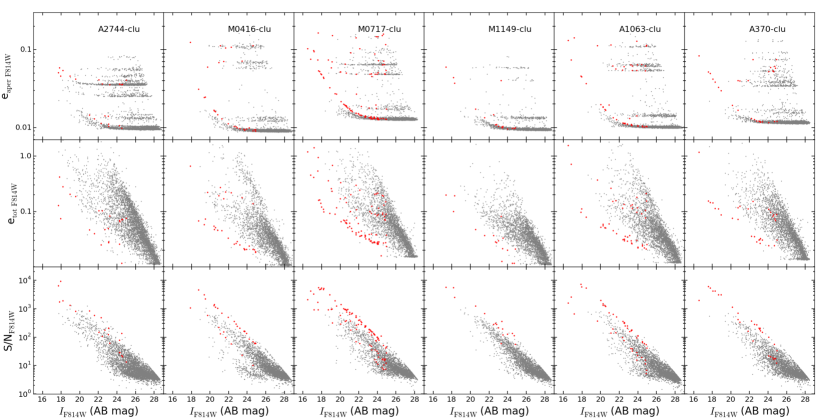
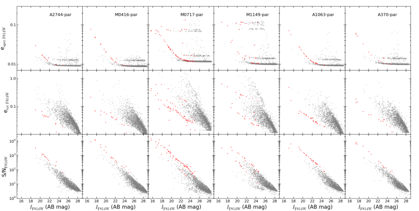
Figure 17.— $F814W$ error distributions in each of the twelve fields. The units are mag${}_{\mathrm{AB}}=-$log(value) + 25. Galaxies defined with use_phot = 1 are shown in gray and point sources in red (star_flag = 1). Top panels: $F814W$ errors within an aperture of $0\farcs 7$ versus magnitude. The variable depths across each mosaic give rise to the discrete levels. Most of the sources fall within the deepest part of the mosaics with photometry aperture errors reaching the lowest values. Middle panels: Total $F814W$ error versus magnitude from the catalogs (see Section 3.5). Bottom panels: Total $F814W$ S/N versus magnitude. In general, point sources have the highest S/N at a given magnitude, while extended sources form the lower envelope of the distribution.

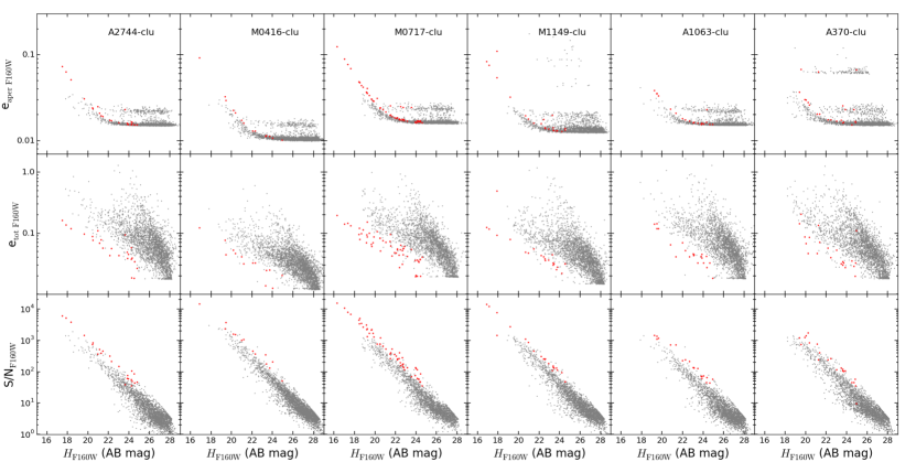
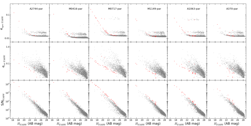
Figure 18.— Same as Figure 17 but for the $F160W$ error distributions in each of the twelve fields with consistent results. The units are mag${}_{\mathrm{AB}}=-$log(value) + 25.

The top panels show the errors in our standard photometric aperture of $0\farcs 7$. The scatter in the error at fixed magnitude is caused by the variation in the depth of the $I_{F814W}$ and the $H_{F160W}$ mosaics. The stripes reflect the weights, and hence the errors, that largely show the depth of a particular position in the mosaic, based on the number of exposures for each source’s position (e.g., see Figure 11). These discrete levels are more prominent in the $I_{F814W}$ mosaics due to more orientations during the observations. Stars (red points) fall in the same bands as galaxies (gray points), as their aperture fluxes are measured in the same $0\farcs 7$ aperture. The distributions differ from field to field, as the depths are not identical. At the bright end, each discrete level turns up from the error being dominated by the Poisson error. In particular, this effect is most obvious for the lowest level of each field.

The middle panels show the “total” errors from the photometry. These errors are determined from the empty aperture errors using the power-law fit at the number of pixels in the circularized Kron aperture (see right panel of Figure 9 and Section 3.5) added in quadrature to the Poisson error for each source, and then scaled to total using the AUTO-to-total flux correction (see Section 3.7). The stripes are blurred in these panels, as the scatter in the error is now dominated by the variation in the Kron aperture size at fixed magnitude and the Poisson error contribution is mostly smoothed out at brighter magnitudes. The range in the Kron aperture sizes reflects the sizes of galaxies at fixed magnitude. Stars (red points) are now offset from galaxies, as the total flux of stars is measured in a smaller aperture than the total flux of extended sources. The estimated errors are smaller for their total fluxes. A few point sources fall within the extended sources envelope at discrete levels in each field (e.g. M0717 and A1063 clusters in Figure 17) due to the empty aperture error being dependent on the depth (see Section 3.5) that varies across the mosaics as discussed previously. These point sources are found in the shallower areas of the mosaics.

In the bottom panels, the S/N of the sources is given as a function of magnitude. The S/N is calculated by dividing the total $I_{F814W}$ and $H_{F160W}$ flux by their respective estimated total error. The relation of the S/N of stars (red points) with magnitude shows very little scatter, demonstrating the small scatter in the errors of stars in the middle panels. Furthermore, the discrete levels persist, from the middle panels, but form tighter sequences similar to the top panels. The errors in the total magnitudes of galaxies are typically much larger and thus have a larger scatter. This should be taken into account when assessing the depth of the $I_{F814W}$ and $H_{F160W}$ mosaics (see Section 3.12).

5. Redshifts, Rest-frame Colors, and Stellar Population Parameters

We use the photometric catalogs to derive photometric redshifts, rest-frame colors, and stellar population parameters of the galaxies for all 12 fields. We note these derived parameters depend significantly on the assumptions and methodology used to derive them (see, e.g., Brammer et al., 2008; Kriek et al., 2009). We choose to use the photometric fitting codes EAZY (Brammer et al., 2008) and FAST (Kriek et al., 2009) to accomplish these tasks. We describe a “default” set of parameters, described below, that we provide with the release of the photometric catalogs. We stress that the released catalogs of the stellar population properties and the rest-frame luminosities do not include the corrections for the lensing magnifications.

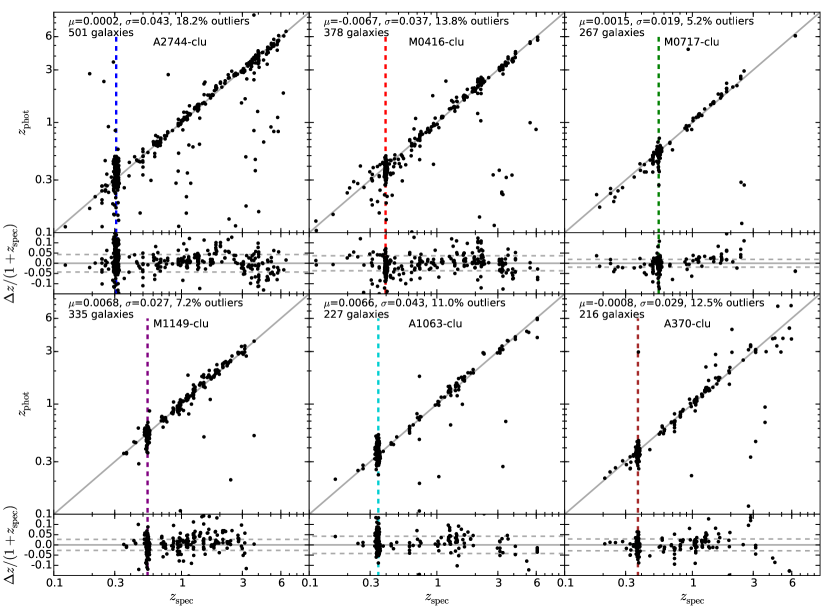
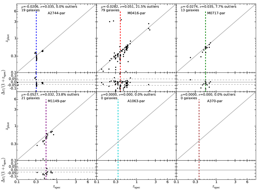
Figure 19.— Comparison of estimated photometric redshifts from our analysis and confirmed published spectroscopic redshifts from the literature for all twelve fields. The bi-weight mean $\mu=(z_{\mathrm{phot}}-z_{\mathrm{spec}})/(1+z_{\mathrm{spec}})$, NMAD scatter $\sigma$, % of objects with $|z_{\mathrm{phot}}-z_{\mathrm{spec}}|/(1+z_{\mathrm{spec}})>0.1$ and the number of galaxies in each comparison are shown in the upper left of the panel for each field. The lower panels of each field show the difference between the photometric and spectroscopic redshifts over $1+z_{\mathrm{spec}}$. The gray dashed lines indicate $\pm\sigma_{\mathrm{NMAD}}$ in each case. The vertical dashed line in each panel indicates the cluster redshift. The gray solid lines in each panel indicate the unity relation between $z_{\mathrm{phot}}$ and $z_{\mathrm{spec}}$.

5.1. Spectroscopic Redshifts

Table 9Spectroscopic Redshift Matches

Field	Matches	Source = “OK” Matches
	(# galaxies)	(# galaxies)
A2744-clu	546	501
A2744-par	22	19
M0416-clu	389	378
M0416-par	80	79
M0717-clu	294	267
M0717-par	17	13
M1149-clu	344	335
M1149-par	22	21
A1063-clu	237	227
A1063-par	0	0
A370-clu	221	216
A370-par	0	0

Note. — Spectroscopic redshift matches from the literature (see Section 5.1). The last column (Source = “OK”) is designating sources with use_phot = 1.

As the HFF cluster and parallel fields are very small areas on the sky, we search the literature to find spectroscopic redshifts of sources that targeted the HFF clusters. These redshifts are used to assess the quality of photometric redshifts in Section 5.2 and used in place of the estimated photometric redshifts, when available, to derive rest-frame colors and stellar population parameters (see Sections 5.3 and 5.4). The spectroscopic redshifts in our catalogs are obtained by cross-matching the positions of sources within $0\farcs 5$ to a number of publicly available catalogs. We select only secure (i.e. reliable according to the reference) spectroscopic redshifts to ensure only quality redshifts are used. However, we have the possibility of sources having multiple references with a spectroscopic redshift. In these cases, we give more weight to references with more robust measurements of the spectroscopic redshift (i.e. a better reported $\delta z$, usually non-grism data). When multiple references are comparable, for the same source, we select the first spectroscopic redshift in our list of references (described below) and cite that reference in the catalog (column REFspecz). This is done for simplicity and does not affect our analysis of derived parameters in the following sections.

The total number of sources with spectroscopic redshifts for each cluster and parallel field and how many of those sources have use_phot = 1 are given in Table 9. We use spectroscopic redshifts from the following literature catalogs: A2744 has five catalogs from GLASS, Brammer et al. (in prep), Mahler et al. (2017), Owers et al. (2011) and Richard et al. (2014); M0416 has seven catalogs from Balestra et al. (2016), Brammer et al. (in prep), Caminha et al. (2016), Ebeling et al. (2014), GLASS, Grillo et al. (2015) and Jauzac et al. (2014); M0717 has four catalogs from Brammer et al. (in prep), Ebeling et al. (2014), GLASS and Limousin et al. (2016); M1149 has five catalogs from Brammer et al. (in prep), Ebeling et al. (2014), GLASS, Grillo et al. (2016) and Smith et al. (2009); A1063 has five catalogs from Brammer et al. (in prep), Diego et al. (2016b), GLASS, Karman et al. (2016) and Richard et al. (2014); and A370 has four catalogs from Brammer et al. (in prep), GLASS, Lagattuta et al. (2016) and Richard et al. (2014). Some of these catalogs utilize previous references that we keep track of and give the original reference, when possible, in our photometric catalogs for the spectroscopic redshift column (REFspecz).

5.2. Photometric Redshifts and Zero Point Corrections

We use the EAZY code (Brammer et al., 2008) to estimate photometric redshifts by fitting the SED of each source with a linear combination of 12 galaxy templates. These templates are derived with the method used for the original EAZY templates (after Blanton & Roweis, 2007), but now using Flexible Stellar Population Synthesis (FSPS) models (Conroy et al., 2009; Conroy & Gunn, 2010) and trained on the UltraVISTA photometric catalogs (Muzzin et al., 2013b). We use the default template error function scaled by a factor of 0.2, which helps to account for systematic wavelength-dependent uncertainties in the templates, and a redshift prior based on the $F160W$ apparent magnitudes.

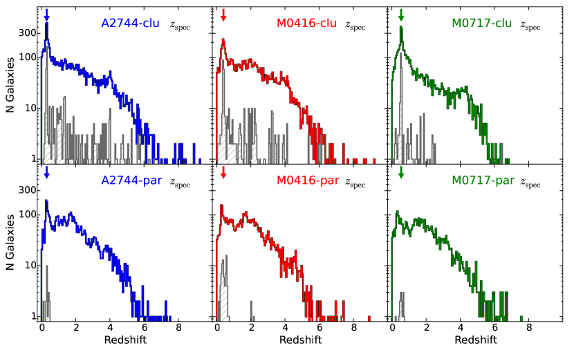
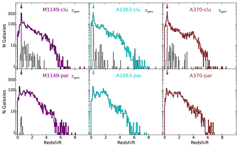
Figure 20.— Redshift distributions of the estimated photometric redshifts (empty histograms) and spectroscopic redshifts (hatched histograms) for the clusters (top) and parallels (bottom) for all HFF. A magnitude cut corresponding to the 90% completeness limits has been applied (utilizing Tables 7 and 8).

Furthermore, we correct the photometry for empirically determined zero point correction factors as in Skelton et al. (2014). Zero point corrections are determined for each band of all fields (see Table 10). We settle on a single set of zero point corrections for all fields due to the small area and limited number of spectroscopic redshifts in each field to determine the zero point corrections from SED fitting. The listed zero point corrections are applied to the catalogs, and the corrected photometry is used for the redshift estimates and stellar population parameters, presented in the following sections. We use the spectroscopic redshift ($z_{\mathrm{spec}}$), if available, or the peak of the photometric redshift distribution (EAZY’s z_peak) as the galaxy redshift, unless otherwise noted.

We find good agreement between the spectroscopic and photometric redshifts by estimating the scatter in each field, the average $\sigma_{\mathrm{nmad}}=0.034$ across all fields with spectroscopic redshifts (A1063 and A370 parallels do not have any spectroscopic redshifts). Figure 19 demonstrates the comparison of the photometric redshifts to spectroscopic redshifts for each field. Among sources with spectroscopic redshifts, there are few outliers (i.e. failures): (18.2, 0.0)%, (13.8, 21.5)%, (5.2, 7.7)%, (7.2, 23.8)%, (11.0, N/A)%, (12.5, N/A)% for A2744, M0416, M0717, M1149, A1063 and A370, respectively, for the clusters and parallels (cluster, parallel), where we define an outlier as $|z_{\mathrm{phot}}-z_{\mathrm{spec}}|/(1+z_{\mathrm{spec}})>$ 0.1. We note that, whereas the mean and sigma in $\Delta z/(1+z_{\mathrm{spec}})$ of the A2744 cluster is quantitatively similar to the other cluster fields, its fraction of outliers is significantly larger. We investigate the SEDs of the outliers in the A2744 cluster, but find no obvious problem with the photometry. No systematic trend is found when $\Delta z/(1+z_{\mathrm{spec}})$ is plotted as a function of the $F160W/F814W$ magnitude of the source or as a function of the brightness of the subtracted model (that includes the background) in either the $F160W$ or the $F814W$ bands. This provides confidence that our bCGs/ICL subtraction does not introduce systematic effects in the derivation of the photometric redshifts.

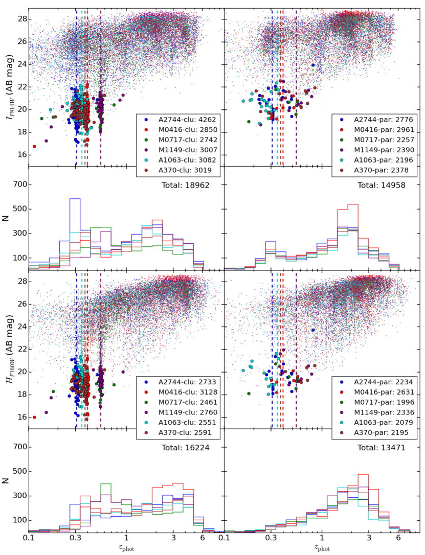
Figure 21.— The distribution of $I_{F814W}$ (top panels) and $H_{F160W}$ (bottom panels) apparent magnitudes with photometric redshift ($z_{\mathrm{peak}}$ from EAZY, $z_{\mathrm{phot}}$ in figure), spectroscopic redshift when available, color-coded by field for both the clusters (left panels) and parallels (right panels). The modeled out bCGs are shown as circles (top panels), color-coded by field the same as the points (see legend in each panel). The lower half of the panels show the number of galaxies as a function of $z_{\mathrm{phot}}$ broken down into the contribution from each field (for sources with use_phot = 1 and “bandtotal” = $F814W$, top panels, and use_phot = 1 with “bandtotal” = $F160W$, bottom panels), again color-coded the same. A magnitude cut corresponding to the 90% completeness limits has been applied (utilizing Tables 7 and 8).

In Figure 20, we show the photometric redshift distributions of sources (selected with use_phot = 1) in each of the fields, using $z_{\mathrm{peak}}$ (open histograms). The spectroscopic redshift distributions are shown by the hashed histograms. For the clusters, the over-densities correspond to the redshift of the cluster as indicated by the peaks in both the $z_{\mathrm{phot}}$ and $z_{\mathrm{spec}}$ distributions. Though clearly less pronounced than in the cluster fields themselves, an excess of galaxies at the cluster redshifts can be seen in the parallel fields $\sim$6 arcmin (1.5$-$2 Mpc) away from the cluster core. These observations are even more evident as the cluster over-densities are illustrated by the distribution of apparent magnitudes with $z_{\mathrm{peak}}$ (see Figure 21, the circles correspond to modeled bCGs) and in the mass distributions (see Figures 24, 25 and Section 5.4). In the lower panel of Fig. 21, we show the number of galaxies as a function of $z_{\mathrm{peak}}$ and give the number of galaxies for each field for $I_{F814W}$ (with use_phot = 1 and bandtotal = $F814W$) and $H_{F160W}$ (with use_phot = 1 and bandtotal = $F160W$).

In Figure 20, we noticed small peaks at a redshift of $z\sim 4$ in a few of the cluster fields (e.g., A2744, M0717 and A370). We investigated this further to determine if there was a problem with the SED fitting resulting in mis-identified sources preferentially placed at $z\sim 4$. We first considered the effect of lensing that may be a likely cause of these $z\sim 4$ peaks as they are not present in the parallel fields and not present at the same redshift in each cluster. We looked at the distribution of galaxies, particularly in the range of $3.5<z<4.5$ for all fields. The galaxies at $z\sim 4$ tend to cluster around the massive galaxies in the cluster as expected from the available lensing maps (see Section 5.5) for the clusters but are mostly distributed evenly in the parallel fields. This is further supported by the fact that we also modeled out bCGs in the parallel fields; suggesting that the apparent enhancement of $z\sim 4$ galaxies in some cluster fields is not due to modeling or SED fitting, but, at least partly, to lensing magnification by the clusters. However, we also explored the possibility that a few of these sources in the clusters could be mis-identified globular clusters (GCs) that become visible after modeling out the bCGs. We selected sources around the very bright massive galaxies in a few of the clusters. The most notable are in the M0416, M0717 and A370 clusters. We selected many of the sources near the modeled out galaxies that have $z_{\mathrm{peak}}\sim 4$ and could potentially be GCs from their spatial distribution, and checked their SEDs and SED fits. Among the objects with reliable modeling of the observed SEDs, only a small fraction of these sources are likely mis-identified GCs with secondary peaks in the EAZY redshift probability functions consistent with the redshifts of the modeled out galaxies. Although we can not rule out some level of contamination from low-redshift GCs to the $z\sim 4$ galaxy population, the mis-identified GCs do not appear to represent a significant contribution to the peaks at $z\sim 4$ noticed in Figure 20, with the A370 cluster having the most possible GC candidates ($<10$ in all). This further supports our conclusion that lensing magnification is likely the main origin of the $z\sim 4$ peaks.

Lastly, we compared our photometric redshifts against the available ASTRODEEP (Merlin et al., 2016; Castellano et al., 2016; Di Criscienzo et al., 2017) catalogs, which have been publicly released for the A2744, M0416, M0717 and M1149 clusters and parallels. To make accurate comparisons as meaningful as possible, we have selected sources based on similar selection criteria (see Figures 28 and 29 in the Appendix for selection criteria). Comparing the redshift histograms in Figure 29, we find qualitatively very similar redshift distributions. In regards to the $z\sim 4$ redshift sources, we find both ours and ASTRODEEP’s distributions show small comparable peaks for the A2744, M0416, M0717 and M1149 clusters. This is further supported by comparing the matched sources’ photometric redshifts, albeit, with some scatter (see Figure 28). The above discussion provides evidence that the peaks at $z\sim 4$ are likely real and due to lensing magnification of the clusters, while mis-identified sources (e.g., GC contamination) are most likely small or negligible contributions to our photometric redshift catalogs.

Table 10Zero Point Corrections for the Hubble Frontier Fields Filters

Filter	Zero Point Correction
UVIS $F225W$	1.1652
$F275W$	0.9855
$F336W$	0.9936
$F390W$	1.0094
ACS $F435W$	1.0352
$F475W$	1.0067
$F555W$	1.0287
$F606W$	1.0105
$F625W$	0.9931
$F775W$	0.9923
$F814W$	0.9990
$F850LP$	0.9999
WFC3 $F105W$	1.0173
$F110W$	1.0178
$F125W$	1.0117
$F140W$	1.0105
$F160W$	$\equiv 1.0$
$K_{S}$    HAWK-I	0.9505
MOSFIRE	1.0221
IRAC $3.6\micron$	1.0464
$4.5\micron$	1.0193
$5.8\micron$	1.0072
$8.0\micron$	0.9970

5.3. Rest-frame Colors

From the photometric catalogs, it is easy to calculate observed colors, but to compare galaxies at different redshifts rest-frame colors need to be used. These can be determined robustly from EAZY as we have a large set of observed-frame photometry in each of the fields. The EAZY templates and best-fitting redshift, spectroscopic redshift if available, are used for each galaxy to determine its rest-frame luminosity in a series of filters. The rest-frame luminosities are calculated individually rather than multiple filters; for more information on how the rest-frame colors are calculated, see Brammer et al. (2011). Along with the photometric catalogs, we provide a catalog that contains the rest-frame luminosities in a variety of commonly used filters (Johnson-Cousins B and R; Johnson-Morgan B; Johnson U, B and V; SDSS ugriz; 2MASS J, H and K; UV 1600 and 2800; Tophat 1400, 1700, 2200, 2700 and 2800).

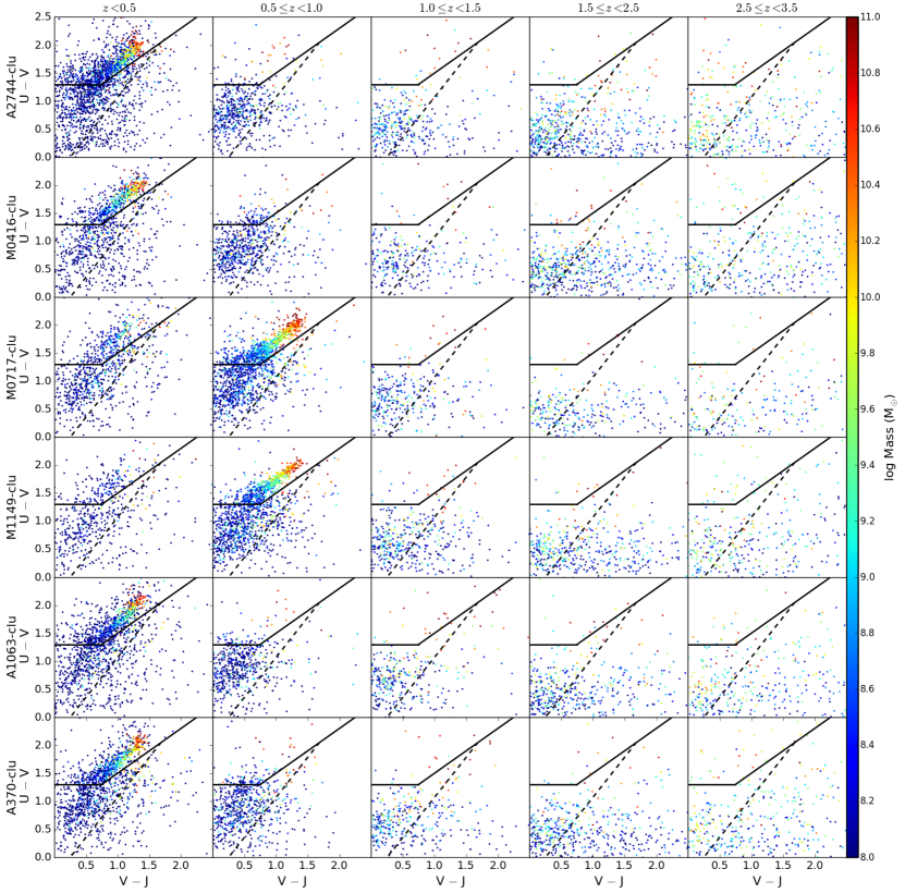
Figure 22.— Color-color selection of the HFF cluster fields. Each row is a different cluster (field name given in vertical axis label), with redshift increasing from left to right (designated at the top of each column). Quiescent and star-forming galaxies are separated by the color-color selection given in Section 5.3 (solid black lines) and the additional selection of dusty star-forming galaxies (dashed black line). The sources (use_phot = 1) are color-coded by the estimated stellar mass for each cluster (color bar on the right side, see Section 5.4). Lensing magnification corrections have not been applied. A magnitude cut corresponding to the 90% completeness limits has been applied (utilizing Tables 7 and 8).

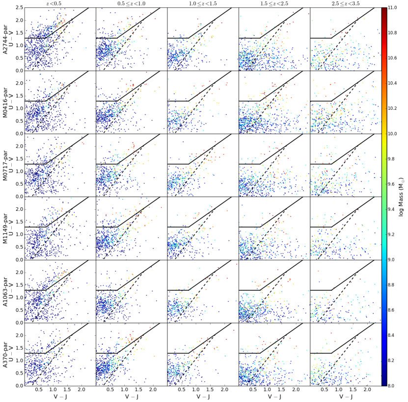
Figure 23.— Same as Figure 22 but for the HFF parallel fields. Lensing magnification corrections have not been applied. A magnitude cut corresponding to the 90% completeness limits has been applied (utilizing Tables 7 and 8).

We can further assess the galaxy populations of each field using a color-color analysis of the rest-frame photometry. For this, we use “UVJ” diagrams (Labbé et al., 2005; Wuyts et al., 2007; Williams et al., 2009) to separate the galaxy population into quiescent and star-forming galaxies for each field. This diagram shows the rest-frame $U-V$ color versus the rest-frame $V-J$ color. In Figures 22 and 23, we use $U-V<1.3$ for $V-J<0.75$ and $U-V<0.8(V-J)+0.7$ for $(V-J)\geq 0.75$ (solid black lines), also for dusty star-forming galaxies $(U-V)<1.43(V-J)-0.36$ (dashed black line, see Martis et al., 2016, for justification of criteria). Each row represents one of the fields, with redshift increasing from left to right, as shown at the top of each column. Quiescent galaxies with low levels of star formation that are red in $U-V$ (upper left region) are separated from similarly red (in $U-V$), dusty star-forming galaxies, with the star-forming galaxies having bluer $U-V$ and $V-J$ colors. Galaxies (selected with use_phot = 1) are color-coded by mass, with the most massive galaxies in red and least massive galaxies in blue (the color bar in the figure at the right gives the stellar mass breakdown). The clusters are identified clearly by a strong quiescent galaxy sequence in their respective redshift bin. The majority of low mass galaxies lie in the star-forming “blue cloud” at all redshifts. In the highest redshift bins ($1.5<z\leq 3.5$) many massive galaxies lie within the star-forming regions and appear to be red due to higher levels of dust rather than older stellar populations.

5.4. Stellar Population Parameters

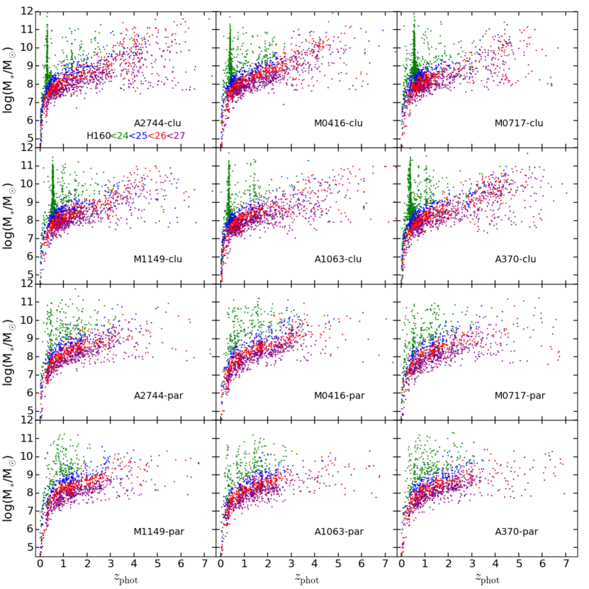
Figure 24.— Photometric redshift versus stellar mass from EAZY and FAST for the $H_{F160W}$ band. The points are color-coded by magnitude, galaxies (use_phot = 1 and “bandtotal” = $F160W$) with $H_{F160W}<24$ are green, $24\leq H_{F160W}<25$ are blue, $25\leq H_{F160W}<26$ are red and $26\leq H_{F160W}<27$ are purple. The over densities seen as peaks (top panels) in photometric redshift correspond to the redshift of the cluster for each of those fields. Lensing magnification corrections have not been applied. A magnitude cut corresponding to the 90% completeness limits has been applied (utilizing Tables 7 and 8).

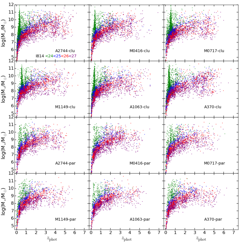
Figure 25.— Same as Figure 24 but for the $I_{F814W}$ band. The points are color-coded by magnitude, galaxies (use_phot = 1) with $I_{F814W}<24$ are green, $24\leq I_{F814W}<25$ are blue, $25\leq I_{F814W}<26$ are red and $26\leq I_{F814W}<27$ are purple. The over densities seen as peaks (top panels) in photometric redshift correspond to the redshift of the cluster for each of those fields. Lensing magnification corrections have not been applied. A magnitude cut corresponding to the 90% completeness limits has been applied (utilizing Tables 7 and 8).

We use the FAST code from Kriek et al. (2009) to estimate stellar masses, star formation rates, ages and dust extinctions, given the photometric redshift from EAZY ($z\_\mathrm{peak}$, see Section 5.2) and the spectroscopic redshift, when available. We use similar input parameters as Skelton et al. (2014). The input parameters are the Bruzual & Charlot (2003) stellar population synthesis model library with a Chabrier (2003) IMF, solar metallicity, exponentially declining star formation histories with a minimum e-folding time of $\log_{10}(\tau/yr)=7$, a minimum age of 10 Myr, $0<A_{V}<6$ mag and the Calzetti et al. (2000) dust attenuation law. Although, we derive star formation rates, dust absorption, and star formation histories for many of the galaxies; we note these quantities are uncertain when derived primarily from optical and near-IR photometry (e.g., see Wuyts et al., 2012b). The stellar population parameters are provided in separate catalogs for each field. The stellar masses and $M/L$ ratios are relatively well-constrained as they mostly depend on the rest-frame optical colors of the galaxies, and these are well-covered by our photometry (observed wavelengths of $0.2-8$ µm).

In Figure 24, we show the distributions of the galaxy stellar masses as a function of the photometric redshift ($z_{\mathrm{peak}}$), for sources that fall within the $F160W$ area. The points are color-coded according to the galaxy’s $H_{F160W}$ magnitude, with the brightest galaxies in green ($H_{F160W}<24$), galaxies with $24\leq$ $H_{F160W}<25$ in blue, galaxies with $25\leq$ $H_{F160W}<26$ in red and galaxies with $26\leq$ $H_{F160W}<27$ in purple. In Figure 25, we show these distributions for all sources with $I_{F814W}$ magnitude (color-coded the same). Again for the cluster fields, we see clearly the over-densities corresponding to the redshift of the clusters with a large population at higher redshifts of relatively bright sources (likely due to lensing of sources by the clusters). For the parallel fields, the distribution is mostly uniform with few very massive galaxies that populate the clusters themselves.

5.5. Lensing Magnifications

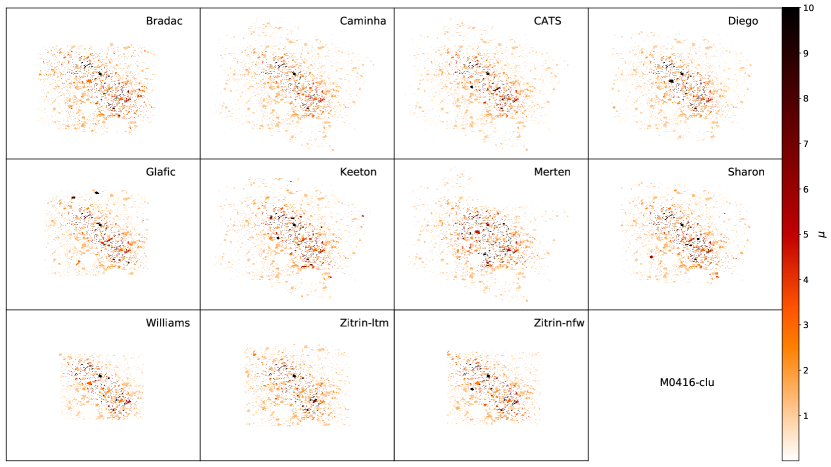
Figure 26.— The magnification factors from the lensing models for each group of the M0416 cluster (see Section 5.5). The produced segmentation map (see Section 3.3) is populated with the derived lensing magnifications specific to each source for the various group’s lensing model (labeled in each panel). The darkest sources are the most heavily magnified and the lightest are the least (the color bar at the right gives the lensing magnification breakdown). It is also worth noting that the coverage areas vary for each group’s lensing model (all other clusters can be found in the Appendix).

We use available lensing models for all the HFF fields to derive magnification values of the sources in our catalogs. Many independent groups have contributed reliable models of the lensing maps for the HFF clusters based on a common set of input data before the HFF observing campaign to help facilitate data analysis. Most of these groups have continued to update the lensing maps to improve and include data from the HFF observing campaign. Several groups assume that the cluster galaxies trace the cluster mass substructure to derive models: the CATS (P.I. Ebeling, e.g. Jauzac et al., 2014), Sharon (e.g. Johnson et al., 2014), (Caminha et al., 2017) use Lenstool, similarly P.I. Keeton using Lensmodel, the GLAFIC model (Oguri, 2010; Ishigaki et al., 2015), and the two different parameterizations (LTM and NFW) provided by the Zitrin team (e.g. Zitrin et al., 2013). Other models that are provided, by P.I.’s Williams (e.g. Grillo et al., 2015), Bradač (e.g. Bradač et al., 2009) and Merten (e.g. Merten et al., 2011), do not assume that cluster mass is traced by its member galaxies but are constrained only by lensing observables. The remaining models, P.I.’s Diego and Bernstein using WSLAP+ (Diego et al., 2005, 2007, 2016a), assume the mass distribution is built as a superposition of Gaussian functions and a compact component that traces the light of the cluster members.

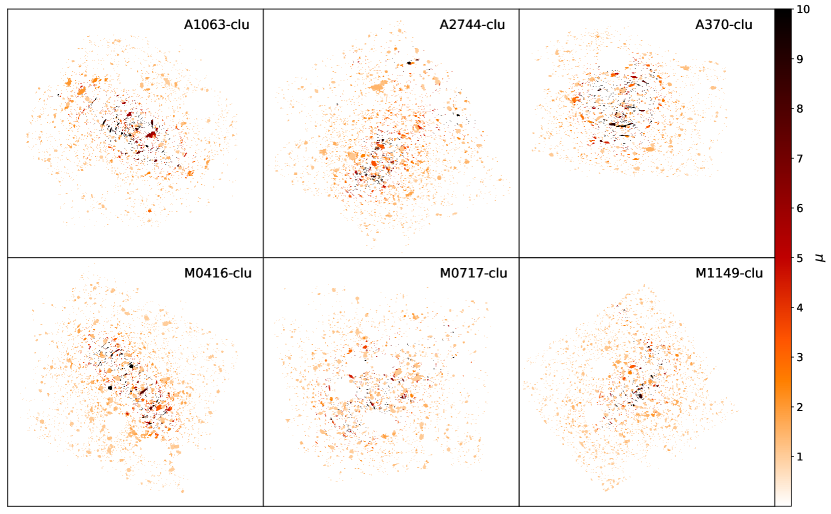
Figure 27.— The magnification factors from the lensing model CATS (arbitrarily chosen) for all six clusters (see Section 5.5). The produced segmentation map (see Section 3.3) for each cluster (labeled in each panel) is populated with the derived lensing magnifications specific to each source. The darkest sources are the most heavily magnified and the lightest are the least (the color bar at the right gives the lensing magnification breakdown).

Each team has provided publicly available shear and mass surface density maps. A detailed description of different models can be found on the HFF lensing website and references therein. Among the available maps only the Merten models partially cover the parallel pointings for some of the fields. For each source, we assign shear ($\gamma$) and mass surface-density ($\kappa$) values by matching the right ascension (RA) and declination (Dec) from our catalogs to the corresponding pixel in the shear and mass maps. Then, we derive the magnification as

$$\mu=\frac{1}{(1-\kappa\times\frac{D_{LS}}{D_{S}})^{2}-(\gamma\times\frac{D_{LS}}{D_{S}})^{2}}$$ (4)

where, $D_{LS}=D_{A}(z_{L},z_{S})$ and $D_{S}=D_{A}(0,z_{S})$ with $D_{A}(0,z_{S})$ being the angular diameter distance to the redshift of the source, and $z_{L}$ being the redshift of the lensing cluster.

In each cluster, we derive lensing magnifications for sources in our catalogs that have an estimated photometric redshift (see Section 5.2), spectroscopic redshift when available, for each group’s most recent lensing model. From this analysis, we include two lensing magnification catalogs for each field in our data release. In both catalogs, each column is a different group’s derived lensing magnification of the sources; one catalog lists errors of the magnification factors derived from the model uncertainties, whereas the other catalog lists the errors of the magnification factors caused by the photometric redshift uncertainties. If a source does not have an estimated photometric redshift, the source is flagged with a $-99$ value. If a source does not fall within the area of the lensing map for each group, the source is flagged with a $-50$ value. For sources with use_phot = 0, these are flagged with a $-1$ value. These flag values are consistent between both lensing magnification catalogs for each field. We leave it up to the user to determine the desired approach for estimating the best magnification of the sources in our photometric catalogs and the various groups’ derived lensing magnifications. We note that the stellar population models derived from FAST and released are not corrected for lensing magnification.

In Figure 26, we show the differences between the lensing models for each group of the M0416 cluster. The produced segmentation map is populated with the derived lensing magnifications specific to each source for the various group’s lensing model (labeled in the figure). The darkest sources are the most heavily magnified and the lightest are the least (the color bar in the figure at the right gives the lensing magnification breakdown). It is also worth noting that the coverage areas vary for each group’s lensing model. Figure 27 shows the derived lensing magnifications for the CATS lensing model of all six clusters (lensing model arbitrarily chosen).

6. Summary

We present the data products and multi-wavelength photometric catalogs produced by the HFF-DeepSpace project for the HFF observing campaign. The survey covers $\sim$165 arcmin² in the six clusters A2744, M0416, M0717, M1149, A1063, A370 and accompanying parallel fields with HST/ACS and HST/WFC3 imaging. The details of the data reduction are given in Section 2.1.2. In addition to the HFF HST data, we include HST/UVIS, ultra-deep $K_{S}$, Spitzer/IRAC and any other available bands from the HST/ACS and WFC3 instruments (see Section 2 and Table 2). We make all the images that have been generated available on our website with the catalogs. Each of the images is on the same astrometric system as the HFF/WFC3 $F160W$ mosaics.

We apply consistent methodology to produce multi-wavelength photometric catalogs and data products for all twelve of the fields. The SExtractor software (Bertin & Arnouts, 1996) is used to detect sources on a noise-equalized combination of the $F814W$, $F105W$, $F125W$, $F140W$ and $F160W$ images. Using the four HFF WFC3 bands and the HFF ACS/$F814W$, we exploit the maximum survey area without sacrificing the depth of the HFF, specifically for the WFC3 bands. As described in Section 3.1, we model out many of the bright cluster members and occasionally other bright sources in the fields. We take great care to achieve accurate cluster models of the bCGs and ICL modeled out ($<1$% uncertainty of the total flux for the bCGs). We carefully measure the flux and errors of the objects in each field and band, taking into account the differences in image resolution between the HST and lower resolution $K_{S}$ and IRAC photometry (see Section 3.5 and 3.6).

Furthermore, we test that the results are consistent for all twelve fields and the total magnitudes and errors agree well with the expected behavior that each source includes only light associated with it (see Section 4). The resulting photometric catalogs span a broad wavelength range from UV to near-IR ($0.2-8$ µm) and are of excellent quality, as demonstrated by the analysis throughout this work. We use EAZY (Brammer et al., 2008) to derive photometric redshifts and achieve an average scatter ($\sigma_{\mathrm{NMAD}}\sim 0.034$) between the photometric and spectroscopic redshifts for all fields with an average significant outlier fraction of $\sim 12$% in all fields (i.e. 10/12 fields, A1063 and A370 parallels do not have any spectroscopic redshift matches). We provide rest-frame colors based on the best-fitting EAZY templates, as well as stellar masses and stellar population parameters for all the galaxies based on fits to their observed photometry (see Section 5) and gravitational lensing magnification factors (see Section 5.5). Furthermore, different methodologies are useful to understand possible systematic uncertainties between various groups’ catalogs of the HFF, as ours are not the only available catalogs (e.g the catalogs of the ASTRODEEP collaboration Merlin et al., 2016; Castellano et al., 2016; Di Criscienzo et al., 2017).

This work, by our HFF-DeepSpace team, concludes the first phase of even more ambitious projects, as outlined in the Introduction. Future work will describe the grism spectroscopy that accompanies these data sets, and help improve the measurements of the redshifts, stellar masses and other stellar properties. Furthermore, these photometric catalogs will be an important aide in designing future surveys as well as planning follow-up programs with current and future observatories (i.e. JWST, GMT, TMT and others) to answer key questions remaining about first light, reionization, the assembly of galaxies and many more topics, most notably, by gaining access to high-redshift sources that are otherwise inaccessible without the strong lensing clusters and power of the HST.

.1. Redshift Distribution Comparisons to Other Catalogs

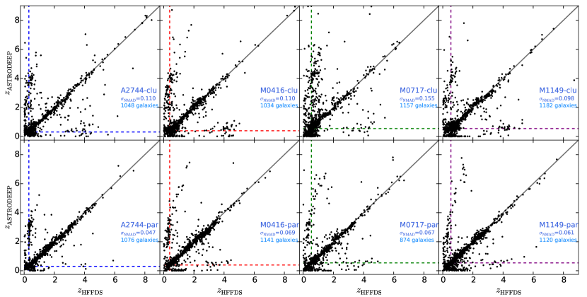
Figure 28.— Comparison of the HFF-DeepSpace photometric redshifts ($z_{\mathrm{HFFDS}}$) to ASTRODEEP ($z_{\mathrm{ASTRODEEP,}}$ Merlin et al., 2016; Castellano et al., 2016; Di Criscienzo et al., 2017). Galaxies were selected to be brighter than AB magnitude of 27 in the $F160W$ band (corresponding roughly to the 90% completeness limit for both catalogs) and matching sources within D$=0.5$ ″. The scatter ($\sigma_{\mathrm{NMAD}}$) and number of matched galaxies are given for each field in their respective panel. The unity relation (solid line) and redshift of the cluster (dashed lines) are marked in each panel.

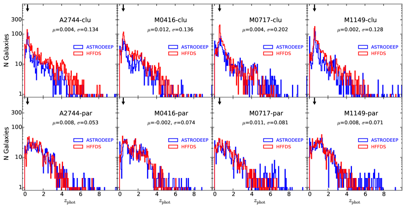
Figure 29.— Histogram comparison of the HFF-DeepSpace photometric redshifts ($z_{\mathrm{phot}}$, red) to ASTRODEEP (blue, Merlin et al., 2016; Castellano et al., 2016; Di Criscienzo et al., 2017). Galaxies were selected to be brighter than AB magnitude of 27 in the $F160W$ band (corresponding roughly to the 90% completeness limit for both catalogs) over comparable source detection areas (i.e., WFC3 footprint of the HFF). The bi-weight mean offset ($\mu$) and scatter ($\sigma$) are given for each field in their respective panel. The black arrow in each panel represents the redshift of the associated cluster.

References

- Balestra et al. (2016) Balestra, I., Mercurio, A., Sartoris, B., et al. 2016, ApJS, 224, 33
- Beers et al. (1990) Beers, T. C., Flynn, K., & Gebhardt, K. 1990, AJ, 100, 32
- Bell et al. (2012) Bell, E. F., van der Wel, A., Papovich, C., et al. 2012, ApJ, 753, 167
- Bertin & Arnouts (1996) Bertin, E. & Arnouts, S. 1996, A&AS, 117, 393
- Blanton & Roweis (2007) Blanton, M. R. & Roweis, S. 2007, AJ, 133, 734
- Bradač et al. (2009) Bradač, M., Treu, T., Applegate, D., et al. 2009, ApJ, 706, 1201
- Brammer et al. (2016) Brammer, G. B., Marchesini, D., Labbé, I., et al. 2016, ApJS, 226, 6
- Brammer et al. (2008) Brammer, G. B., van Dokkum, P. G., & Coppi, P. 2008, ApJ, 686, 1503
- Brammer et al. (2011) Brammer, G. B., Whitaker, K. E., van Dokkum, P. G., et al. 2011, ApJ, 739, 24
- Bruzual & Charlot (2003) Bruzual, G. & Charlot, S. 2003, MNRAS, 344, 1000
- Calzetti et al. (2000) Calzetti, D., Armus, L., Bohlin, R. C., et al. 2000, ApJ, 533, 682
- Caminha et al. (2016) Caminha, G. B., Grillo, C., Rosati, P., et al. 2016, A&A, 587, A80
- Caminha et al. (2017) —. 2017, A&A, 600, A90
- Castellano et al. (2016) Castellano, M., Amorín, R., Merlin, E., et al. 2016, A&A, 590, A31
- Chabrier (2003) Chabrier, G. 2003, PASP, 115, 763
- Chang et al. (2013) Chang, Y.-Y., van der Wel, A., Rix, H.-W., et al. 2013, ApJ, 773, 149
- Connor et al. (2017) Connor, T., Donahue, M., Kelson, D. D., et al. 2017, ApJ, 848, 37
- Conroy & Gunn (2010) Conroy, C. & Gunn, J. E. 2010, ApJ, 712, 833
- Conroy et al. (2009) Conroy, C., Gunn, J. E., & White, M. 2009, ApJ, 699, 486
- Di Criscienzo et al. (2017) Di Criscienzo, M., Merlin, E., Castellano, M., et al. 2017, ArXiv e-prints
- Diego et al. (2016a) Diego, J. M., Broadhurst, T., Chen, C., et al. 2016a, MNRAS, 456, 356
- Diego et al. (2016b) Diego, J. M., Broadhurst, T., Wong, J., et al. 2016b, MNRAS, 459, 3447
- Diego et al. (2005) Diego, J. M., Protopapas, P., Sandvik, H. B., et al. 2005, MNRAS, 360, 477
- Diego et al. (2007) Diego, J. M., Tegmark, M., Protopapas, P., et al. 2007, MNRAS, 375, 958
- Duncan et al. (2014) Duncan, K., Conselice, C. J., Mortlock, A., et al. 2014, MNRAS, 444, 2960
- Ebeling et al. (2014) Ebeling, H., Ma, C.-J., & Barrett, E. 2014, ApJS, 211, 21
- Ferrarese et al. (2006) Ferrarese, L., Côté, P., Jordán, A., et al. 2006, ApJS, 164, 334
- Franx et al. (2008) Franx, M., van Dokkum, P. G., Förster Schreiber, N. M., et al. 2008, ApJ, 688, 770
- González et al. (2014) González, V., Bouwens, R., Illingworth, G., et al. 2014, ApJ, 781, 34
- González-López et al. (2017) González-López, J., Bauer, F. E., Romero-Cañizales, C., et al. 2017, A&A, 597, A41
- Grazian et al. (2015) Grazian, A., Fontana, A., Santini, P., et al. 2015, A&A, 575, A96
- Grillo et al. (2016) Grillo, C., Karman, W., Suyu, S. H., et al. 2016, ApJ, 822, 78
- Grillo et al. (2015) Grillo, C., Suyu, S. H., Rosati, P., et al. 2015, ApJ, 800, 38
- Hatch et al. (2016) Hatch, N. A., Muldrew, S. I., Cooke, E. A., et al. 2016, MNRAS, 459, 387
- Hsu et al. (2017) Hsu, L.-Y., Desai, V., Murphy, E. J., et al. 2017, ApJ, 840, 29
- Ishigaki et al. (2015) Ishigaki, M., Kawamata, R., Ouchi, M., et al. 2015, ApJ, 799, 12
- Jauzac et al. (2014) Jauzac, M., Clément, B., Limousin, M., et al. 2014, MNRAS, 443, 1549
- Johnson et al. (2014) Johnson, T. L., Sharon, K., Bayliss, M. B., et al. 2014, ApJ, 797, 48
- Karman et al. (2016) Karman, W., Grillo, C., Balestra, I., et al. 2016, A&A, 585, A27
- Kriek et al. (2009) Kriek, M., van Dokkum, P. G., Labbé, I., et al. 2009, ApJ, 700, 221
- Labbé et al. (2006) Labbé, I., Bouwens, R., Illingworth, G. D., et al. 2006, ApJ, 649, L67
- Labbé et al. (2005) Labbé, I., Huang, J., Franx, M., et al. 2005, ApJ, 624, L81
- Labbé et al. (2015) Labbé, I., Oesch, P. A., Illingworth, G. D., et al. 2015, ApJS, 221, 23
- Lagattuta et al. (2016) Lagattuta, D. J., Richard, J., Clément, B., et al. 2016, ArXiv e-prints
- Laporte et al. (2017) Laporte, N., Bauer, F. E., Troncoso-Iribarren, P., et al. 2017, A&A, 604, A132
- Limousin et al. (2016) Limousin, M., Richard, J., Jullo, E., et al. 2016, A&A, 588, A99
- Lotz et al. (2017) Lotz, J. M., Koekemoer, A., Coe, D., et al. 2017, ApJ, 837, 97
- Ly et al. (2015) Ly, C., Rigby, J. R., Cooper, M., et al. 2015, ApJ, 805, 45
- Mahler et al. (2017) Mahler, G., Richard, J., Clément, B., et al. 2017, ArXiv e-prints
- Maier et al. (2015) Maier, C., Ziegler, B. L., Lilly, S. J., et al. 2015, A&A, 577, A14
- Marchesini et al. (2009) Marchesini, D., van Dokkum, P. G., Förster Schreiber, N. M., et al. 2009, ApJ, 701, 1765
- Martis et al. (2016) Martis, N. S., Marchesini, D., Brammer, G. B., et al. 2016, ApJ, 827, L25
- Merlin et al. (2016) Merlin, E., Amorín, R., Castellano, M., et al. 2016, A&A, 590, A30
- Merten et al. (2011) Merten, J., Coe, D., Dupke, R., et al. 2011, MNRAS, 417, 333
- Montes & Trujillo (2014) Montes, M. & Trujillo, I. 2014, ApJ, 794, 137
- Muzzin et al. (2013a) Muzzin, A., Marchesini, D., Stefanon, M., et al. 2013a, ApJ, 777, 18
- Muzzin et al. (2013b) —. 2013b, ApJS, 206, 8
- Muzzin et al. (2013c) Muzzin, A., Wilson, G., Demarco, R., et al. 2013c, ApJ, 767, 39
- Muzzin et al. (2008) Muzzin, A., Wilson, G., Lacy, M., et al. 2008, ApJ, 686, 966
- Nantais et al. (2016) Nantais, J. B., van der Burg, R. F. J., Lidman, C., et al. 2016, A&A, 592, A161
- Oguri (2010) Oguri, M. 2010, PASJ, 62, 1017
- Oke (1971) Oke, J. B. 1971, ApJ, 170, 193
- Owers et al. (2011) Owers, M. S., Randall, S. W., Nulsen, P. E. J., et al. 2011, ApJ, 728, 27
- Pacifici et al. (2016) Pacifici, C., Kassin, S. A., Weiner, B. J., et al. 2016, ApJ, 832, 79
- Papovich et al. (2012) Papovich, C., Bassett, R., Lotz, J. M., et al. 2012, ApJ, 750, 93
- Papovich et al. (2011) Papovich, C., Finkelstein, S. L., Ferguson, H. C., et al. 2011, MNRAS, 412, 1123
- Peng et al. (2010) Peng, C. Y., Ho, L. C., Impey, C. D., et al. 2010, AJ, 139, 2097
- Pérez-González et al. (2008) Pérez-González, P. G., Rieke, G. H., Villar, V., et al. 2008, ApJ, 675, 234
- Pope et al. (2017) Pope, A., Montaña, A., Battisti, A., et al. 2017, ApJ, 838, 137
- Postman et al. (2012) Postman, M., Coe, D., Benítez, N., et al. 2012, ApJS, 199, 25
- Rawle et al. (2016) Rawle, T. D., Altieri, B., Egami, E., et al. 2016, MNRAS, 459, 1626
- Richard et al. (2014) Richard, J., Jauzac, M., Limousin, M., et al. 2014, MNRAS, 444, 268
- Salmon et al. (2015) Salmon, B., Papovich, C., Finkelstein, S. L., et al. 2015, ApJ, 799, 183
- Shivaei et al. (2015) Shivaei, I., Reddy, N. A., Shapley, A. E., et al. 2015, ApJ, 815, 98
- Skelton et al. (2014) Skelton, R. E., Whitaker, K. E., Momcheva, I. G., et al. 2014, ApJS, 214, 24
- Smith et al. (2009) Smith, G. P., Ebeling, H., Limousin, M., et al. 2009, ApJ, 707, L163
- Song et al. (2016) Song, M., Finkelstein, S. L., Ashby, M. L. N., et al. 2016, ApJ, 825, 5
- Tomczak et al. (2016) Tomczak, A. R., Quadri, R. F., Tran, K.-V. H., et al. 2016, ApJ, 817, 118
- Tomczak et al. (2014) —. 2014, ApJ, 783, 85
- Tremonti et al. (2004) Tremonti, C. A., Heckman, T. M., Kauffmann, G., et al. 2004, ApJ, 613, 898
- Treu et al. (2015) Treu, T., Schmidt, K. B., Brammer, G. B., et al. 2015, ApJ, 812, 114
- van der Wel et al. (2012) van der Wel, A., Bell, E. F., Häussler, B., et al. 2012, ApJS, 203, 24
- van Dokkum (2001) van Dokkum, P. G. 2001, PASP, 113, 1420
- van Weeren et al. (2017) van Weeren, R. J., Ogrean, G. A., Jones, C., et al. 2017, ApJ, 835, 197
- Webb et al. (2015) Webb, T. M. A., Muzzin, A., Noble, A., et al. 2015, ApJ, 814, 96
- Whitaker et al. (2011) Whitaker, K. E., Labbé, I., van Dokkum, P. G., et al. 2011, ApJ, 735, 86
- Whitaker et al. (2012) Whitaker, K. E., van Dokkum, P. G., Brammer, G., et al. 2012, ApJ, 754, L29
- Williams et al. (2009) Williams, R. J., Quadri, R. F., Franx, M., et al. 2009, ApJ, 691, 1879
- Wuyts et al. (2012a) Wuyts, E., Rigby, J. R., Sharon, K., et al. 2012a, ApJ, 755, 73
- Wuyts et al. (2012b) Wuyts, S., Förster Schreiber, N. M., Genzel, R., et al. 2012b, ApJ, 753, 114
- Wuyts et al. (2007) Wuyts, S., Labbé, I., Franx, M., et al. 2007, ApJ, 655, 51
- Yabe et al. (2012) Yabe, K., Ohta, K., Iwamuro, F., et al. 2012, PASJ, 64, 60
- Zahid et al. (2014) Zahid, H. J., Kashino, D., Silverman, J. D., et al. 2014, ApJ, 792, 75
- Zitrin et al. (2013) Zitrin, A., Meneghetti, M., Umetsu, K., et al. 2013, ApJ, 762, L30