Pileup mitigation at the LHC

A theorist’s view

Grégory Soyez
Institut de Physique Théorique, CNRS, CEA Saclay, Université Paris-Saclay,

Orme des Merisiers, Bât 774, F-91191 Gif-sur-Yvette cedex, France

email: gregory.soyez@ipht.fr

Abstract

To maximise the potential for new measurements and discoveries at CERN’s Large Hadron Collider (LHC), the machine delivers as high as possible collision rates. As a direct consequence, multiple proton-proton collisions occur whenever two bunches of protons cross. Interesting high-energy (hard) collisions are therefore contaminated by several soft, zero-bias, ones. This effect, known as pileup, pollutes the final state of the collision. It complicates the reconstruction of the objects in this final state, resulting in increased experimental measurement uncertainties.

To reduce these uncertainties, and thus improve the quality and precision of LHC measurements, techniques are devised to correct for the effects of pileup. This document provides a theoretical review of the main methods employed during Run I and II of the LHC to mitigate pileup effects. I will start with an in-depth presentation of the area–median used for the vast majority of applications, including several refinements of the original idea, their practical (numerical) implementation and an assessment of their efficiency and robustness. I will then focus on several theoretical calculations that can provide both quantitative and qualitative information on the area–median approach.

In the specific case of boosted jets, a field that has seen a wide interest recently, a set of methods, known as grooming techniques has also been used. I will describe these techniques, address their performance and briefly show that they are amenable to a theoretical, analytic, understanding.

The last part of this review will focus on ideas oriented towards future pileup mitigation techniques. This includes a couple of new methods that have recently been proposed as well as a large series of alternative ideas. The latter are yet unpublished and have not received the same amount of investigation than the former but they have the potential to bring new developments and further improvement over existing techniques in a future where pileup mitigation will be crucial.

Chapter 1 Introduction

Collider physics has played a central role in fundamental research over the past decades. Today, most earth-based experiments exploring particle physics at high energies are beam–beam collider experiments with the Large Hadron Collider (LHC) occupying the front row. This type of experiment brings into collision two beams of particles, either leptons or hadrons. The topic of this review applies to proton-proton collisions, with applications for the on-going LHC programme as the main focus. As we will show, it also has consequences for heavy-ion collisions such as the gold–gold collisions at RHIC — the Relativistic Heavy-Ion Collider at the Brookhaven National Laboratory — or lead–lead collisions at the LHC. The physics discussed here is even more relevant for future hadronic colliders. From now on, let us consider the collision of two proton beams.

The primary goal of the LHC is to explore physics at high energies — or, equivalently, short distances — typically around the TeV scale (i.e. around $10^{-19}$ m or $10^{-4}$ fm). The vast majority of the analyses at the LHC involve either measurements of standard-model processes or searches for new phenomena involving physics beyond the standard model. Given the constraints already obtained from earlier colliders such as the Tevatron or LEP, the LHC analyses explore either energy (kinematic) domains previously unreachable, or rare phenomena in extreme corners of the phase-space, or both.

With collisions at a centre-of-mass energy of 13 TeV, the LHC is able to boldly probe energies that no collider had probed before. This is however not sufficient to explore rare corners of the phase space for which we also need to accumulate as much data as possible. For this one wants to reach the highest possible collision rate. To understand how it works in practice, it is interesting to look a bit closer at how the LHC works. Each beam is made of trains of bunches ($\sim 2800$ bunches per beam at the LHC), where each bunch contains billions of protons ($\sim 10^{11}$ at the LHC). There are several ways to maximise the collision rate: increase the number of bunches, increase the number of protons per bunch, or improve the beam optics so that the beams are better focalised at the interaction points (technically, lowering the $\beta^{*}$ parameter). The net effect of increasing the number of protons per bunch or improving the beam optics is that whenever two bunches cross at one of the interaction points (i.e. in one of the experiments), the rate of collisions increases, to a point that several proton-proton collisions occur simultaneously, during one bunch crossing. It is this effect of simultaneous collisions which is called pileup and which is the main topic of this review.

To be more quantitative, the collision rate of a collider is called the luminosity ${\cal{L}}$, and can be measured in $\text{cm}^{-2}\text{s}^{-1}$. Towards the end of Run II of the LHC, the machine delivers a luminosity around $2\,10^{34}\,\text{cm}^{-2}\text{s}^{-1}$, twice its nominal value. For a process with a cross-section $\sigma$, the rate of events for this process is ${\mathcal{L}}\sigma$. For example, the total cross-section for the production of a $t\bar{t}$ pair is around $800$ pb and that for a Higgs boson is around $50$ pb, resulting in about 15 $t\bar{t}$ pairs produced per second and one Higgs boson per second at the current luminosity. More generally, the LHC typically studies processes with a cross-section that can go as low a few femtobarns, i.e. 11-14 orders of magnitude lower than the total proton-proton cross-section.

To estimate the pileup multiplicity, i.e. the number of proton-proton interactions occurring per bunch crossing, one also needs the number of bunches or, equivalently, the time separation between two bunches. At the LHC it is 25 ns. The luminosity ${\mathcal{L}}=2\,10^{34}\,\text{cm}^{-2}\text{s}^{-1}$ therefore corresponds to a luminosity per bunch crossing ${\mathcal{L}}_{\text{crossing}}=5\,10^{26}\,\text{cm}^{-2}=0.5\,\text{mb}^{-1}$. Given a total proton-proton cross-section of order 100 mb, this gives around 50 proton-proton interactions per bunch crossing, i.e. an average pileup multiplicity $\left\langle{N_{\mathrm{PU}}}\right\rangle\sim 50$. Pileup itself is not really a new issue: it was already present at the Tevatron, albeit with a much lower multiplicity (typically around 5), so that simple techniques were sufficient to address its effects. It is with the LHC and its large luminosity that pileup multiplicities started to crank up. The average pileup multiplicity was already around $\left\langle{N_{\mathrm{PU}}}\right\rangle\sim 20$ during Run I [1] and 30 at the beginning of Run II. For the coming high-luminosity LHC (HL-LHC) one expects an average pileup multiplicity between 140 and 200 [2, 3]. Note that, in practice, the actual number of interactions in a given bunch crossing, $N_{\mathrm{PU}}$, fluctuates, following a Poisson distribution around its average $\left\langle{N_{\mathrm{PU}}}\right\rangle$.

Imagine now that during a collision we have one of those high-energy (hard) rare processes that the LHC experiments are keen to study. A number of other, simultaneous, zero-bias collisions will occur during the same bunch crossing. The overall final-state of the collision, observed in the detectors, is therefore not only the products of one hard collision we are interested in, but the superposition of these products with those of all the simultaneous soft collisions. In other words, the final-state of the collision includes both the final-state particles of the hard collision and pileup. Since zero-bias (pileup) proton-proton collisions typically produce a few tens of soft hadrons in their final-state, the net result of pileup is to add hundreds to thousands of soft hadrons to the final-state of the hard collision one wishes to study (referred to as “the hard event” or “the hard collision” in what follows).

Now that we have described what pileup is, we can discuss what its effect are. In a nutshell, adding a large number of soft particles to the final-state of the collision complicates the reconstruction of the properties of the hard event itself. To better understand this, remember that pileup is essentially made of a large number of soft hadrons, spread over the whole detector. The reconstruction of any object involving the hadrons produced in the final-state of the collision will therefore be affected by this additional hadronic activity.

Probably the most typical situation where pileup impacts the ability to properly reconstruct the objects in the final-state of a hard collision is the case of jets. Jets are the collimated sprays of hadrons stemming from the showering and hadronisation of the high-energy partons produced in the hard collision (we refer to Ref. [4] for a relatively recent review and Appendix A for a quick overview). The hadrons from pileup will overlap with those of the hard collision so that when jets are reconstructed, particles of the former will be clustered together with particles of the latter. In other words, a given jet will have both particles from the hard event and from pileup. The properties of the hard jets — mostly the jet transverse momentum but also its rapidity and azimuthal angle — will be biased by these extra hadrons coming from pileup.

Jets are not the only objects to be affected by pileup: every object whose reconstruction involves the hadrons in the final state of the collision will be. This covers almost all the objects one uses in LHC analyses. Reconstructing leptons and photons usually involves a condition on the hadronic activity in the surroundings of the lepton/photon. This activity will obviously be affected by the extra hadrons from pileup. Missing transverse energy is accessed by reconstructing the transverse momentum of all the measured objects in the event. This will obviously be affected by the extra hadrons from pileup. Tagging $B$ hadrons (using displaced vertices or other kinematic variables), or even reconstructing the particles in the final-state from the output of the detector, also involves hadronic information. This will also be affected by the extra hadrons from pileup.

Generally speaking the practical consequences of pileup are two-folded. The first effect is almost straightforward: pileup biases the quantities measured from the final state. For example, the transverse momentum of jets is shifted upwards due to the extra hadronic activity; or the hadronic energy around a lepton/photon is increased, resulting in a loss of reconstruction efficiency. The second effect is a little bit more subtle and is related to the fact that the pileup activity fluctuates. These fluctuations arise from multiple reasons: the actual number of pileup events, ${N_{\mathrm{PU}}}$, fluctuates around its average $\left\langle{N_{\mathrm{PU}}}\right\rangle$; then, the final-state hadronic activity fluctuates from one zero-bias collisions to another. The last point takes several forms: the overall (total) energy deposited in the final state fluctuates between different zero-bias collisions but the distribution of these particles across the detector changes as well. As a consequence, the energy deposited by the pileup particles will vary in different regions of the detector as well as other properties like, for example, the relative fraction of charged and neutral particles coming from pileup. All these fluctuations yield a smearing of the quantities reconstructed from the final state of the collision: fluctuations of the pileup activity will result in fluctuations of the bias due to pileup, i.e. a smearing of the reconstructed quantities and distributions. For example, the reconstructed jet transverse momentum will be smeared by the fluctuating pileup activity, affecting the jet energy resolution. Similarly, the resolution on the missing transverse energy will degrade due to the fluctuations of the overall pileup activity. In summary, pileup biases and smears the quantities reconstructed from the final state of the hard collision, with the latter resulting in a degradation of the resolution. We will discuss this more precisely in Section 2.1.

To gain a little more insight on the importance of pileup effects, one can give a quick quantitative estimate of the above effects (see chapter 3 for a more precise discussion). For 13 TeV collisions and a pileup multiplicity of 50, which is representative of the situation towards the end of Run II of the LHC, an anti-$k_{t}$ jet of radius $R=0.4$ will see its energy shifted, on average, by 15-20 GeV, with a smearing of about 7 GeV. Now imagine that one wants to reconstruct jets down to a few tens of GeV, say 20-30 GeV, e.g. for the measurement of double Higgs production (a key element of the LHC programme). Both the energy shift and smearing are becoming serious issues. Even if this is an extreme example, it is good to keep in mind that the energy scales of pileup effects when reconstructing jets is not negligible, typically in the 10-GeV ballpark (a little above for the bias, a little below for the smearing) and will increase at the HL-LHC. This is therefore something one cannot neglect and has to be addressed in almost all the analysis at the LHC. Pileup often turns out to be one of the important sources of systematic uncertainties at the LHC. This affects in particular precision measurements, or measurements involving lower energy scales.

Given the harmful effects of pileup, it is natural to investigate how to mitigate them. This exercise naturally means pursuing two goals: (i) correcting for its biases and (ii) reducing its damaging effects on resolution. Addressing pileup mitigation techniques is the main purpose of this review. For this, it is important to keep in mind the above two goals, especially when it will come to assessing the performance of pileup mitigation tools.

Note that one could always take the attitude that pileup is part of the detector effects on observables and that one could correct for its effects using an unfolding procedure (as one typically does for other detector effects), without applying any specific pileup mitigation technique. This can be reinforced by the fact that a proper measurement would anyway have to unfold for detector effects, as well as for residual pileup effects after one applies (or not) a pileup mitigation technique. There are several reasons to believe that there is an added value to applying carefully-designed pileup mitigation techniques. In our opinion, the main argument in favour of pileup mitigation techniques is that it provides a more generic (observable-independent) and precise approach than a global unfolding. As we shall discuss in Section 2.1, and show repeatedly throughout this review, pileup mitigation techniques aim at reducing as much as they can the biases and resolution-degradation effects of pileup by exploiting event-by-event, and even jet-by-jet, information. This procedure is, to a very large extent, independent of the details of a specific observable or distribution one wants to measure. After these “in-situ” corrections one is therefore left with much smaller residual corrections to apply and one should therefore expect that this ultimately leads to smaller systematic uncertainties compared to a situation where all pileup corrections would have been left to an a posteriori unfolding procedure. In other words, by first applying an efficient pileup mitigation method — reducing the average biases and improving the resolution in each event in a generic way independent of the details of the analysis — the analysis-dependent unfolding that one is left with is much lighter, hence most likely resulting in smaller and better-controlled systematic uncertainties.

That said, we should keep in mind that, for precision measurements, one would still need an unfolding of the residual pileup effects. On the one hand this means that one can live with small residual biases (see also discussions in Chapter 9), but on the other hand, it also means that we want to keep these residual corrections small and process-independent and that we want, for example, to avoid fluctuations with long tails which are more delicate to unfold.

Over the past decade several pileup mitigation techniques have been proposed. One of the first proposed methods for used at the LHC relied on the ability to reconstruct quite efficiently pileup vertices using charged tracks. It applied a correction directly proportional to the number of reconstructed pileup vertices. Ultimately, Run I of the LHC has adopted instead the area–median method, initially proposed [5] by Matteo Cacciari and Gavin Salam, and significantly extended by Matteo Cacciari, Gavin Salam and myself [6, 7, 8, 9, 10]. this method has still extensively been used during Run II except in specific applications to which we will return later. As we will show at length in this document, one of the benchmarks of the area–median method is that it provides an efficient and robust way to correct for pileup, with a sizeable reduction of the resolution degradation and a very small remaining average bias. However, with the perspective for yet higher pileup multiplicities in the future, several groups have started to investigate yet more powerful techniques, yielding several new methods like cleansing [11], the SoftKiller [12], PUPPI [13] or a wavelet approach [14], or machine-learning-based techniques like PUMML[15] or PUPPIML [16].

In this context, this document serves several purposes. The first and main one (part I of this document) is to provide a review of the area–median method that is used at the LHC. This includes an extensive discussion of the method itself, and its application to several observables, including the ubiquitous jet transverse momentum, the jet mass and jet shapes, and the jet fragmentation function. We will also perform an in-depth Monte-Carlo validation of the approach for applications at the LHC and highlight our recommendation for practical use of the area–median pileup subtraction technique. Since pileup subtraction is most often done numerically, we will also include a description of the area–median interface provided in FastJet [17, 18].

Another aspect that will be explored in the context of our review of the area–median method is its application to heavy-ion collisions either in gold–gold collisions at RHIC or in lead–lead collisions at the LHC. Even though in both cases luminosities are sufficiently low to neglect pileup effects, the case of heavy-ion collisions has a different effect that behaves similarly to pileup: the quark–gluon plasma created during a heavy-ion collision decays into a large number (thousands) of particles in the final-state of the collision, corresponding to a huge Underlying Event activity. This is in practice very similar to pileup, with many soft particles scattered all over the event and compromising the reconstruction of the hard objects in the event. The activity of the Underlying Event in a LHC lead–lead event is even larger than the current pileup activity at the LHC: for the most central collisions, an anti-$k_{t}$ jet of radius $R=0.4$ can receive an additional contamination of $100-150$ GeV, with fluctuations above 15 GeV. We will therefore review as well how the area–median can be used to correct for the large Underlying Event contamination to jets produced in heavy-ion collisions. This however requires a few words of caution. First of all, the Underlying Event cannot practically be separated from the “hard event” in a well-defined way (this is also the case in proton–proton collisions). In heavy-ion terms, the medium and jet particles cannot be uniquely separated, the jet can for example back-react on the medium, … Additionally, the products of the decay of the quark–gluon plasma have flow structures, like the elliptic flow (see e.g.  [19, 20, 21, 22, 23, 24, 25, 26, 27]), related to the geometry of the collision, which need to be taken into account when implementing a correction.

Besides a thorough description of the area–median pileup subtraction method, we also wish to present a series of other results and techniques. These will cover two main directions. The first (part II of this document) concerns a family of methods used in the specific context of jet substructure. Jet substructure, used e.g. for the identification of boosted objects, is an entire topic on its own and we will focus here on the aspects related to pileup mitigation. One of the important aspects here is that jet substructure studies typically use fat jets, i.e. large-radius jets, which are specially affected by pileup (and the Underlying Event). Our focus here will be centred on grooming techniques which aim at limiting the overall sensitivity of jets to pileup. As we shall argue e.g. in Chapter 7), grooming techniques take a relatively orthogonal approach to pileup mitigation compared to the area–median method. They reduce the sensitivity to pileup — basically by using an effective jet radius smaller than the one of the original fat jet — without explicitly correcting for pileup effects. For better results, grooming techniques should therefore be supplemented by a pileup correction like the area–median method, or the Constituent Subtractor [28] (a particle-based extension of the area–median approach), or PUPPI [13] (developed and used extensively by CMS for substructure analyses during Run II of the LHC). Our goal here is to focus on the grooming aspects, so our studies will use them in conjunction with the area–median approach.

Finally, in the third and last part of this document, we will discuss methods that have been proposed more recently and which aim at reducing the sensitivity to pileup fluctuations and their impact on the jet energy resolution. These methods are mostly meant for future use, typically at the HL-LHC and potential future hadronic colliders, where the pileup conditions will significantly worsen.

Our aim in this last part is not to provide an exhaustive review of existing methods. In particular, we will not discuss recent tools such as PUPPI (except for some comparisons in our conclusive study) or machine-learning-based approaches such as PUMML or PUPPIML. Instead, we mainly target two goals. The first is to highlight the challenges of the exercise. In particular, we will argue that improving on the resolution front is usually done at the expense of a more limited control over the bias of the method (cf. the two goals of pileup mitigation introduced earlier). This will be contrasted with the area–median approach. We will for example study the SoftKiller (which makes use of key quantities of the area–median method). We shall also discuss the applicability of the area–median subtraction method to charged-hadron-subtracted (CHS) type of events and compare it to an alternative approach which directly makes use of the ratio of charged tracks to neutral energy deposits.

The second goal of this third part is to document a series of yet unpublished results. These mostly cover ideas and candidates for new pileup mitigation methods organised in two series of studies: one concerning the possibility to use grooming techniques as a generic tool for pileup subtraction (not confined to their applications to fat jets); the other covering a list of candidates for event-wide pileup mitigation methods that we have come across when developing the SoftKiller. In all these cases, the idea is to explore different methods that can lead to a reduction of the pileup fluctuation effects on jet energy resolution. Only a few methods have been proposed so far and our hope here is that the series of preliminary results we present can help towards building more powerful tools in the future.

Before getting our hands dirty, one last point needs to be addressed in this introduction: as stated in the title of this review, we concentrate on theoretical aspects of pileup mitigation and this calls for clarifications. Based on what is said above, one can easily get the feeling that pileup is a purely experimental issue. After all, reconstructing the fundamental objects in the final state of a collision seems exclusively an experimental task connected to a proper understanding of all aspects of the detector’s response. We want to show here that there is more to the story and that there is room for theoretical ideas and concepts when it comes to investigating pileup effects and pileup mitigation.

To highlight this, we will provide analytic insights on our results whenever possible throughout this document. (See the “reading guide” below to navigate between descriptions, results, Monte Carlo simulations and analytic details.) In the first part, related to the review of the area–median approach, we will discuss pileup effects using simple analytic arguments. We will also show that the concept of jet areas [29], central to the area–median method, has lots of interesting features in perturbative Quantum Chromodynamics (QCD), observed as well in Monte Carlo simulations. The main features of the other central ingredient of the area–median method, namely the event-by-event estimate of the pileup activity, can also be understood from a simple toy-model of pileup for which we can obtain a series of analytic results.

Furthermore, analytic results can also be obtained for the grooming techniques discussed in the second part of this document. The fact that jet substructure techniques can be amenable to an analytic understanding has been one of the major breakthrough in the jet substructure community over the past few years. It has even been shown that they are nice candidates for precision calculations at the LHC (see e.g.  [30, 31, 32, 33, 34]). In Chapter 8, we will give a few insights into analytic calculations for grooming techniques, focusing primarily on quantities related to pileup.

Conversely, since the main purpose of this document is to focus on the theoretical aspects of pileup mitigation, we will extensively use Monte Carlo simulations but we will not at all discuss additional complications related to detector effects or other effects like out-of-time pileup which comes from the fact that the detectors readout often spans over the time of several bunch crossings. To be fully addressed, these effects need a dedicated experimental analysis, with details specific to each experiments, which goes beyond the scope of this document. It is however worth mentioning that, as far as the area–median pileup subtraction technique is concerned, we are confident that the picture described here is not going to be strongly affected by detector effects. This is mainly due to that fact that the area–median method is extremely robust against the details of both the hard and the pileup events. For the same reason, we shall concentrate our discussion on the reconstruction of the properties of the jets. Other quantities like lepton/photon isolation criteria or missing-$E_{T}$ reconstruction are much more dependent on the details of the detectors and will not be investigated here. Readers who are interested in experimental aspects of pileup subtraction can for example consult Ref. [35] for the ATLAS experiment of Ref. [36] for CMS.

Reading guide and organisation of this document.

Even without entering into the details of detector effects, this document remains rather long. We therefore find helpful to give a short reading guide through this review.

We first reiterate that this document focuses only on pileup mitigation. A brief description of the commonly-used jet algorithms is given in Appendix A and we refer to Ref. [4] for a comprehensive introduction to jet physics in general. That said, we have separated the text in three main parts: first the extensive description of the area–median method, followed by a discussion of grooming techniques in the second part and, finally, opening towards more recent techniques in the third part of this document. I strongly suggest to all readers to go through the first two Sections of Chapter 2 which provide a generic description of pileup effects, generic considerations about pileup mitigation and the net effects on physical observables. These two Sections also introduce basic pileup characteristics that will be used throughout the whole document e.g. to provide physical interpretations of our results.

The discussion of the area–median method has been organised in three different steps: we describe the method and its several extensions in Chapter 2, we provide a validation of the method based on Monte Carlo simulations in Chapters 3 (pileup in proton-proton collisions) and 4 (Underlying Event in heavy-ion collisions) and introduce a series of analytic results in Chapter 5. Again, the reader interested in the area–median method is invited to go first through Chapter 2 and in particular through Section 2.4, which gives the basic description of the method, and Section 2.8, which lists in details our practical recommendations for use at the LHC. Some of the more technical aspects like the definition of jet areas (Section 2.3), extensions to jet shapes (Section 2.5) and jet fragmentation function moments (Section 2.6), or the practical details of the FastJet interface (Section 2.7) can be skipped if one is just interested in the main lines. Chapter 3 then demonstrates the performance of the method, justifying the recommendations made in Section 2.8, with Chapter 4 departing from pure pileup mitigation to concentrate of the application of the area–median method to the subtraction of the large Underlying Event in heavy-ion collisions. Our overview of the area–median method ends with Chapter 5 where we discuss at length analytic properties of jet areas, and provide a brief translation of the analytic results of [37], initially discussing the analytic estimation of the Underlying Event activity, to the estimation of the pileup properties.

The second and third parts of this document cover more specialised topics. For the discussion of grooming techniques applied to boosted jets (the second part of this document), we have kept the same structure as for the first part: we first provide a detailed description of a series of grooming methods (Chapter 6), then move on to a series of Monte Carlo studies (Chapter 7) and finish with a description of a few analytic results for groomers (Chapter 8). The reader who is not familiar with grooming is obviously invited to read first the descriptions in Chapter 6. The Monte Carlo studies (Chapter 7) mostly revisit a study done in the context of the Boost 2012 workshop [38], studying how groomers mitigate pileup for boosted jets. However, the study presented here extends the one originally done for the Boost proceedings to include a more extensive and modern set of grooming techniques. At last, Chapter 8 will provide a calculation of the grooming radius, directly related to the sensitivity to pileup, for the SoftDrop [39] grooming procedure. This is merely an example illustrating how jet substructure methods are amenable to an analytic treatment. This Chapter is more appropriate for the reader who is curious about recent developments aiming towards an analytic understanding of jet substructure.

The third part of this document will discuss several methods going beyond the area–median approach. We encourage all readers to explore Chapter 9 which provides an introductory discussion of the motivations to seek for more powerful techniques as well as the associated fundamental challenges. For readers interested in continuing their journey in this direction, we have then split the results in four separate chapters that can be read more-or-less independently. We start in Chapter 10 with a preliminary study of the usage of grooming techniques as a generic tool for pileup mitigation, beyond the scope of boosted jets. Then, in Chapter 11, we discuss the use of CHS events and charged tracks information to help mitigating pileup contamination for neutral particles. This includes a discussion of the area–median method and the “Neutral-proportional-to-Charged” method [10] as well as an in-depth comparison to the recently proposed cleansing technique [11]. In Chapter 12 we introduce the SoftKiller method that shows significant improvements over the area–median method in terms of energy resolution, while keeping limited average biases. We believe that it can be a powerful method for use in high-pileup environments, especially in view of its remarkable speed properties. Finally, in Chapter 13 we list a series of preliminary studies including several event-wide subtraction methods that we have only briefly investigated when we were developing the SoftKiller method, as well as possible extensions of the SoftKiller method itself. These are still preliminary results but I believe that they can prove helpful in the development of future pileup mitigation methods.

As a conclusion, we will provide a summary of the key performances of several methods, published and preliminary, using the common framework that had been introduced in the context of the PileUp WorkShop held at CERN in May 2014 [40]. This part is also appropriate for a generic reader who can then go back and dig more into the additional details he or she would be interested in.

Part I The area–median approach

Chapter 2 Description of the area–median method

2.1 Basic characterisation of the pileup effects

Before discussing how to remove the pileup contamination from a jet it is helpful to characterise that contamination in terms of a few simple physical effects. This simple characterisation has its limitations but provides a simple physical understanding of many situations we shall discuss throughout this document.

The most fundamental case we will focus on is the reconstruction of the jet transverse momentum, $p_{t}$. This is by far the most used jet characteristic. Applications to more generic jet properties will be discussed in Sections 2.5 and 2.6.

The main characteristic of pileup that the area–median approach makes use of is the fact that, in each event, the energy (or, rather, the transverse momentum) deposit coming from pileup is to a large extent uniform in rapidity and azimuth. In that approximation the pileup activity is characterised by a single number: the pileup transverse momentum density, $\rho$. In this framework, $\rho$ is defined per unit of area in the rapidity–azimuth plane. It is crucial to point out that, here, $\rho$ is defined event by event. In practice, $\rho$ has a additional relatively small rapidity dependence, smooth on average. For the sake of this discussion, let us temporarily neglect that dependence. We will come back to it in Section 2.4.2.

Given the pileup transverse momentum density $\rho$, the pileup effect on a jet will be to shift its $p_{t}$ by an amount proportional to $\rho$. Since $\rho$ is defined per unit area in the rapidity–azimuth plane, the proportionality constant will be the “area” of the jet, $A_{\rm jet}$. If one thinks of a calorimeter with towers of size $a\times a$, this is equivalent to saying that the $p_{t}$ of a jet will be shifted by the average pileup $p_{t}$ in each tower, $\rho_{\rm tower}$, times the number of towers in the jet, $N_{\rm towers}$. In our language, this corresponds to $\rho_{\rm tower}=\rho a^{2}$ with a jet areas $A_{\rm jet}=N_{\rm towers}a^{2}$.

We will discuss at length the generic definition of the area of a jet in the next section. In a nutshell, the idea is to add to a given event a dense and uniform coverage of infinitely soft particles, ghosts, each carrying a quantum of area $a_{\rm ghost}$. We then define the active area of a jet as the number of ghosts in the jet, multiplied by $a_{\rm ghost}$. Physically, this active area mimics the effect of pileup in the sense that pileup particles are uniformly distributed, in the limit where their $p_{t}$ becomes infinitely small. This last point ensures that ghosts do not affect the clustering provided one uses an infrared-safe jet algorithm.

For a given pileup density $\rho$ and jet area $A_{\rm jet}$, the average effect due to the clustering of pileup particles in a jet is to shift the jet $p_{t}$ by $\rho A_{\rm jet}$.

A series of additional effects come on top of the simple transverse momentum shift discussed above. The fact that the pileup transverse momentum deposit is uniform in rapidity and azimuth is just an approximation only true on average. If one takes an event with a given $\rho$ one can imagine looking at the energy deposit in a square patch of size $1\times 1$ in the rapidity–azimuth plane. As this patch moves in the event the energy deposit will vary. This results in a full distribution which is interesting in itself but, for most of the simple discussions in this document, it is sufficient to see it as a Gaussian of average $\rho$ and standard deviation $\sigma$. This new pileup property, $\sigma$, characterises the pileup fluctuations within an event and will appear each time we discuss the uncertainty of pileup subtraction techniques.

The effect of the pileup fluctuations on the jet is to smear its transverse momentum. Indeed, if the jet sits on an upwards (resp. downwards) pileup fluctuation, the contamination due to the capture of pileup particle in the jet will be more (resp. less) than the average $\rho A_{\rm jet}$. These fluctuations around $\rho A_{\rm jet}$ are given by $\sigma\sqrt{A_{\rm jet}}$. The proportionality to $\sigma$ is expected but the appearance of $\sqrt{A_{\rm jet}}$ may be a bit more of a surprise. This is actually the fact that fluctuations, i.e. dispersion of statistical distributions, add in quadrature, which means that it is $\sigma^{2}$ which scales like the area of the jet. Another, perhaps more concrete, way to see this is to come back to the case of a calorimeter. If the pileup $p_{t}$ in towers fluctuates by an amount $\sigma_{\rm tower}$, the $p_{t}$ fluctuations in a jet of $N_{\rm towers}$ towers will be $\sigma_{\rm tower}\sqrt{N_{\rm towers}}$. If we take a patch of area 1 in which there is $1/a^{2}$ towers, this gives $\sigma_{\rm tower}=\sigma a$ and, remembering $A_{\rm jet}=N_{\rm towers}a^{2}$, we get fluctuations in our jet given by $\sigma\sqrt{A_{\rm jet}}$.

Before turning to the discussion of how pileup affects the jet $p_{t}$, there is a third effect that one has to introduce: back-reaction (BR). This relates to the fact that pileup does not just add extra soft particles, from pileup interactions, to jets: since pileup particles are clustered at the same time as particles from the hard interaction, the particles from the hard interactions clustered in a given jet can be affected by the presence of the pileup particles. Back-reaction is the difference between the clustering done with and without pileup particles, computed only using the particles from the hard interactions within a given jet . Again, the effect of back-reaction on the jet transverse momentum is both an average shift and a dispersion. We will provide detailed calculations and simulations of back-reaction effects in Section 5.1.3, but all that we need to know at this stage is that if one uses the anti-$k_{t}$ algorithm [41] to cluster the jets, the average $p_{t}$ shift due to back-reaction is negligible and its smearing effects are proportional to $\sqrt{\rho p_{t}}$ with a relatively small coefficient which make them relevant only at large $p_{t}$.

The discussion so far can be summarised under the form of a pocket formula which will be extremely useful for many discussions throughout this report: the effect of pileup on the jet transverse momentum is given by

$$\boxed{\,p_{t,\rm full}=p_{t,\rm hard}+\rho A_{\rm jet}\pm\sigma\sqrt{A_{\rm jet}}+{\rm BR},\,}$$ (2.1)

where $p_{t,\rm full}$ is the transverse momentum of the jet when clustering the event with particles from both the hard interaction and pileup, while $p_{t,\rm hard}$ is the jet $p_{t}$ with only the hard particles, i.e. the quantity we really want to reconstruct. In the rhs of this equation, the second term (the $\rho$ term) is the average shift, the third term (the $\sigma$ term) is the pileup fluctuations, responsible for degrading the jet energy resolution, and the fourth is the back-reaction effects, all introduced above. We will see these effects directly in Monte-Carlo simulations in Chapter 3. Similar considerations also apply to other jet properties, with $\rho$ shifting their average value and $\sigma$ smearing their value (see e.g. Section 2.5 for additional details).

For the sake of future discussions, it is helpful to introduce a few additional quantities. When averaging over an ensemble of events, we will denote the average of $\rho$ by $\left\langle\rho\right\rangle_{\rm ev}$ and its standard deviation by $\sigma_{\rho}$. It is also customary to see the pileup as a superposition of $N_{\mathrm{PU}}$  minimum bias events. Each minimum bias event has itself a corresponding $\rho\equiv\rho_{\rm mb}$ and $\sigma=\sigma_{\rm mb}$. We shall denote its average by $\left\langle\rho_{\rm mb}\right\rangle_{\rm ev}$ and its standard deviation by $\sigma_{\rho,\rm mb}$. For a class of events with the same $N_{\mathrm{PU}}$, we would have, neglecting the fluctuations across the event sample of all the various $\sigma$,

$$\left\langle\rho\right\rangle_{\text{ev, fixed }{N_{\mathrm{PU}}}}={N_{\mathrm{PU}}}\left\langle\rho_{\rm mb}\right\rangle_{\rm ev},\qquad\sigma_{\text{ev, fixed }{N_{\mathrm{PU}}}}=\sqrt{{N_{\mathrm{PU}}}}\,\sigma_{\rm mb}\quad\text{ and }\quad\sigma_{\rho\text{, fixed }{N_{\mathrm{PU}}}}=\sqrt{{N_{\mathrm{PU}}}}\,\sigma_{\rho,{\rm mb}}.$$ (2.2)

Of course, if one averages over all events, one also needs to take into account the variations of $N_{\mathrm{PU}}$ across events. The dispersion of $\rho$ will then pick an extra contribution coming from the variation of $N_{\mathrm{PU}}$. This gives

$$\left\langle\rho\right\rangle_{\rm ev}=\mu\left\langle\rho_{\rm mb}\right\rangle_{\rm ev},\qquad\sigma=\sqrt{\mu}\,\sigma_{\rm mb}\quad\text{ and }\quad\sigma_{\rho}^{2}\simeq\mu\sigma^{2}_{\rho,{\rm mb}}+\sigma^{2}_{N_{\mathrm{PU}}}\left\langle\rho_{\rm mb}\right\rangle_{\rm ev}^{2}$$ (2.3)

where, we have defined $\mu$ as the average number of pileup interactions and $\sigma_{N_{\mathrm{PU}}}$ its standard deviation. For a Poison-distributed pileup, we have $\sigma_{N_{\mathrm{PU}}}^{2}=\mu$.

From these considerations, we can reformulate Eq. (2.1) in several ways:

$$p_{t,\rm full} =p_{t,\rm hard}+\left\langle\rho_{\rm mb}\right\rangle_{\rm ev}{N_{\mathrm{PU}}}A_{\rm jet}\pm\sigma_{\rho,\rm mb}\sqrt{{N_{\mathrm{PU}}}}A_{\rm jet}\pm\sigma\sqrt{A_{\rm jet}}+{\rm BR}$$ (2.4)

$$=p_{t,\rm hard}+\left\langle\rho_{\rm mb}\right\rangle_{\rm ev}\mu A_{\rm jet}\pm\left\langle\rho_{\rm mb}\right\rangle_{\rm ev}\sqrt{\mu}A_{\rm jet}\pm\sigma_{\rho,\rm mb}\sqrt{\mu}A_{\rm jet}\pm\sigma\sqrt{A_{\rm jet}}+{\rm BR}$$ (2.5)

These expressions differ in the level at which we compute the average shift and fluctuations:

• in (2.1), the average shift is characterised by $\rho$, defined event by event, leaving the intra-event fluctuations $\sigma$;

• in (2.4) the average shift is proportional to the number of pileup vertices and we therefore get an extra source of fluctuations, $\sigma_{\rho,\rm mb}\sqrt{{N_{\mathrm{PU}}}}A_{\rm jet}$, coming the fact that the fluctuations in the overall pileup deposit of each minbias event will translate in fluctuations in $\rho$;

• in (2.5), the average shift is written as a constant $p_{t}=\left\langle\rho_{\rm mb}\right\rangle_{\rm ev}\mu A_{\rm jet}$ for each jet of area $A_{\rm jet}$ and we pick yet an extra source of smearing coming from the fluctuations of $N_{\mathrm{PU}}$, $\left\langle\rho_{\rm mb}\right\rangle_{\rm ev}\sqrt{\mu}A_{\rm jet}$.

As we shall see in this Chapter and the following ones, various pileup mitigation techniques subtract from the full jet transverse momentum and estimate of the average shift. One would then be left with residual fluctuations depending on the level at which this is done. These various expressions will prove useful when we discuss the net bias and residual resolution degradation after we apply a pileup subtraction technique.

These basic considerations are almost enough to introduce the area–median subtraction method but a few subtleties arise from our definition of the jet area. We shall therefore introduce that concept once and for all in Section 2.3 and return to the area–median subtraction method in Section 2.4.

Note finally that for all the applications that we will consider in this document, we can assume some form of ordering between the various quantities introduced above. Typically, the scale of the hard jet will be larger than the background contamination, itself larger than the pileup fluctuations, namely, $p_{t,\rm hard}/A_{\rm jet}>\rho>\sigma$. This approximation is valid for the case of pileup at the LHC.

2.2 Effects of average shifts and resolution degradation on physical observables

We have seen that the main effects of pileup are to shift and smear the transverse momentum of the jets, as well as their other kinematic properties. The goal of pileup mitigation is, to a large extent, to correct for the average shift and to reduce as much as possible the smearing effects. At many stages in this document, we will characterise pileup subtraction techniques using these properties as quality measures.

In order to put things in perspective and to facilitate the understanding of several arguments used when we will discuss our findings, it is helpful to provide a simple description of the effects that an average shift and a dispersion would have on physical observables.

For the sake of the argument, let us consider the differential jet cross-section as a function of the jet transverse momentum, $d\sigma/dp_{t}$. Imagine this has a truth distribution $d\sigma_{\rm truth}/dp_{t}$ corresponding to a case without pileup, usually denoted by $d\sigma_{\rm hard}/dp_{t}$ throughout this document. Let us now add pileup to that initial distribution and, optionally, subtract it, to obtain a “reconstructed” jet cross-section $d\sigma_{\rm reco}/dp_{t}$. This is the result of the convolution of the initial, truth, spectrum with the spectrum characterising the residual pileup effects. We want to understand how this will differ from the expected result $d\sigma_{\rm truth}/dp_{t}$.

For the vast majority of the results discussed here, several simplifications can be made. First, the effect of pileup and the optional additional subtraction can, to a large extent, be approximated by a Gaussian of average $\Delta$ and of dispersion $\sigma$. The former corresponds to the average shift, or bias, or offset, while the latter corresponds to the residual smearing, or resolution degradation, or fluctuations. As long as the residual effects of pileup do not show long tails the Gaussian approximation is appropriate to capture the physics.

Then, let us approximate the initial distribution by a decreasing exponential:

$$\frac{d\sigma_{\rm truth}}{dp_{t}}=\frac{\sigma_{0}}{\kappa}e^{-p_{t}/\kappa}.$$ (2.6)

This is representative of a steeply-falling distribution and, as long as $\Delta$ and $\sigma$ are not too large, it is always a good approximation, at least locally.

If we convolute that distribution with a Gaussian, we find

$$\frac{d\sigma_{\rm reco}}{dp_{t}} \approx\int dk_{t}\frac{1}{\sqrt{2\pi}\sigma}e^{-\frac{(p_{t}-k_{t}-\Delta)^{2}}{2\sigma^{2}}}\frac{d\sigma_{\rm truth}}{dk_{t}}$$ (2.7)

$$\approx\frac{d\sigma_{\rm truth}}{dp_{t}}\exp\left(\frac{\Delta}{\kappa}+\frac{\sigma^{2}}{2\kappa^{2}}\right).$$ (2.8)

The above result shows that both the average shift and the dispersion have an impact on the final reconstructed distribution. The effect of the shift is rather trivial: an offset $\Delta$ on $p_{t}$ translates immediately in a factor $\exp(\Delta/\kappa)$. The effect of the dispersion is a bit more subtle. It is related to the fact than, on a steeply-falling distribution, positive fluctuations will be given a larger weight than negative fluctuations.

An alternative way to see this is to look, for a given reconstructed $p_{t,\rm reco}$, at the distribution of the initial, truth, $p_{t,\rm truth}$. This is given by

$$P(p_{t,\rm truth}|p_{t,\rm reco}) =\left[\frac{d\sigma_{\rm reco}}{dp_{t,\rm reco}}\right]^{-1}\frac{1}{\sqrt{2\pi}\sigma}e^{-\frac{(p_{t,\rm reco}-p_{t,\rm truth}-\Delta)^{2}}{2\sigma^{2}}}\frac{d\sigma_{\rm truth}}{dp_{t,\rm truth}}$$ (2.9)

$$=\frac{1}{\sqrt{2\pi}\sigma}\exp\left[-\frac{1}{2\sigma^{2}}\left(p_{t,\rm truth}-p_{t,\rm reco}+\Delta+\frac{\sigma^{2}}{\kappa}\right)^{2}\right].$$ (2.10)

This shows that the most probable truth $p_{t}$ is given by

$$p_{t,\rm truth}^{\text{(most likely)}}=p_{t,\rm reco}-\Delta-\frac{\sigma^{2}}{\kappa}.$$ (2.11)

The presence of the $\Delta$ shift here is again expected and we see that we get an extra contribution coming from the dispersion. This extra contribution increases if the initial distribution becomes steeper (i.e. when $\kappa$ decreases) and disappears for a flat distribution ($\kappa\to\infty$).

From the above perspective, one sees that if we want to mitigate pileup, the ideal situation would be to have both $\Delta$ and $\sigma$ as small as possible. From Eq. (2.8), we see that having $\Delta+\sigma^{2}/(2\kappa)=0$ would also translate into an unbiased reconstructed distribution but this requires some level of fine-tuning and would be process-dependent. In practice, we typically target pileup mitigation techniques that result in $\Delta\approx 0$, and try to reduce $\sigma$ as much as possible. In an experimental context, the effect of $\sigma$ (and the residual $\Delta$) would ultimately have to be unfolded together with the other detector effects.

The discussion in this Section has only taken the jet $p_{t}$ and the jet cross-section as an example. The very same arguments can be made for other processes and for other jet properties. As long as the residual effect of pileup are small enough, they can reasonable be approximated by a Gaussian distribution and the physical observable can locally be approximated by a decreasing exponential. In these conditions, the results (2.8) and (2.10) would therefore apply and capture most of the relevant effects to estimate pileup effects and to assess the quality of pileup mitigation techniques.

Finally, this discussion also justifies that the average shift and dispersion are the two basic quality measures to study and, up to very few exceptions, we will do so in all our studies in this document. The robustness of a method can be assessed by checking that the average shift $\Delta$ remains close to 0 regardless of the physical process under consideration, the scale of the hard process, the pileup conditions and other jet properties like its rapidity. Once the robustness of a method is established, we can discuss its efficiency in terms of how small the residual smearing $\sigma$ is.

2.3 The jet catchment areas

The first ingredient we will need for the area–median pileup subtraction method is the definition of the concept of jet areas. This concept can be seen as an additional property of each jet, like their transverse momentum or mass. Note that, for hadronic collisions, we work with the transverse momentum ($p_{t}$), rapidity ($y$), azimuthal angle ($\phi$) coordinate system and by “jet area” we really mean the area in the $y-\phi$ plane.

In the context of a (simple) calorimeter, it is natural to think of the area of a jet as the sum of the areas of each of the cells included in the jet. In a sense, our goal in this Section is to provide a well-defined concept of jet areas which would also work at particle-level and remain well-defined in the case of a calorimeter with empty towers in a jet. Naively, one could just say that the area of a jet of radius $R$ should be $\pi R^{2}$ which would be biased because not all jet algorithms produce circular jets and the boundary of a jet can be influenced by the surrounding jets. Another tempting definition would be to take the convex hull of all the particles constituting the jet. Again, this is not an ideal choice since convex hulls could overlap and would not pave the rapidity–azimuth plane. In a nutshell, our solution is to define the area of a jet as a catchment area, i.e. the region of the rapidity–azimuth plane where the jet would catch infinitely soft particles. There are several ways to implement this in practice, hence we will introduce three definitions: the passive area, the active area and the Voronoi area.

For reasons that will soon become clear, the active area is the most appropriate for pileup subtraction but we will start our discussion with the passive area since it is the most simple one. Finally, jet areas are amenable to analytic calculations and we shall discuss this in great detail in Section 5.1.

2.3.1 Passive Area

Suppose we have an event composed of a set of particles $\{p_{i}\}$ which are clustered into a set of jets $\{J_{i}\}$ by some infrared-safe jet algorithm.

Imagine then adding to the $\{p_{i}\}$ a single infinitely soft ghost particle $g$ at rapidity $y$ and azimuth $\phi$, and repeating the jet-finding. As long as the jet algorithm is infrared safe, the set of jets $\{J_{i}\}$ is not changed by this operation: their kinematics and hard particle content will remain the same, the only possible differences being either the presence of $g$ in one of the jets or the appearance of a new jet containing only $g$.

The passive area of the jet $J$ can then either be defined as a scalar

$$a(J)\equiv\int dy\,d\phi\;f(g(y,\phi),J)\qquad\qquad f(g,J)=\left\{\begin{array}[]{cc}1&g\in J\\ 0&g\notin J\\ \end{array}\right.\;,$$ (2.12)

which corresponds to the area of the region where $g$ is clustered with $J$, or as a 4-vector,

$$a_{\mu}(J)\equiv\int dy\,d\phi\;f_{\mu}(g(y,\phi),J)\qquad\qquad f_{\mu}(g,J)=\left\{\begin{array}[]{cc}g_{\mu}/g_{t}&g\in J\\ 0&g\notin J\\ \end{array}\right.\;,$$ (2.13)

where $g_{t}$ is the ghost transverse momentum. For a jet with a small area $a(J)\ll 1$, the 4-vector area has the properties that its transverse component satisfies $a_{t}(J)=a(J)$, it is roughly massless and it points in the direction of $J$. For larger jets, $a(J)\sim 1$, the 4-vector area acquires a mass and may not point in the same direction as $J$. We shall restrict our attention here to scalar areas because of their greater simplicity. Nearly all results for scalar areas carry over to 4-vector areas, modulo corrections suppressed by powers of the jet radius (usually accompanied by a small coefficient).

2.3.2 From passive to Voronoi area

The only algorithm for which one can make any statement about the passive area for a general $n$-particle configuration is the $k_{t}$ algorithm [45, 46].

Because of the $k_{t}$ distance measure, the single ghost will cluster with one of the event particles before any other clustering takes place. One can determine the region in which the ghost will cluster with a given particle, and this is a definition of the area $a_{k_{t},R}(p_{i})$ of a particle $p_{i}$. Since the ghost-particle clustering will occur before any particle-particle clustering, the jet area will be the sum of the areas of all its constituent particles:

$$a_{k_{t},R}(J)=\sum_{p_{i}\in J}a_{k_{t},R}(p_{i})\,.$$ (2.15)

Can anything be said about the area of a particle? The ghost will cluster with the event particle to which it is closest, as long it is within a distance $R$. This corresponds to a geometrical construction known as the Voronoi diagram, which subdivides the plane with a set of vertices into cells around each vertices. Each cell has the property that all points in the cell have as their closest vertex the cell’s vertex. Thus the Voronoi cell is equivalent similar to the region in which a ghost will cluster with a particle up to the limitation that the ghost should be within a distance $R$ of the particle. This leads us to define the Voronoi area of particle $i$, $a_{R}^{{\cal V}}(p_{i})$, to be the area of its Voronoi cell ${\cal V}_{i}$ intersected with a circle of radius $R$, ${\cal C}_{i,R}$, centred on the particle:

$$a_{R}^{{\cal V}}(p_{i})\equiv\text{area}({\cal V}_{i}\cap{\cal C}_{i,R})\,.$$ (2.16)

Thus given a set of momenta, the passive area of a $k_{t}$ jet can be directly determined from the Voronoi diagram of the event, using Eq. (2.15) and the relation

$$a_{k_{t},R}(p_{i})=a_{R}^{{\cal V}}(p_{i})\,.$$ (2.17)

Figure 2.1: The passive area of jets in a parton-level event generated by Herwig and clustered with the $k_{t}$ algorithm with $R=1$. The towers represent calorimeter cells containing the particles, the straight (green) lines are the edges of the Voronoi cells and the shaded regions are the areas of the jets.

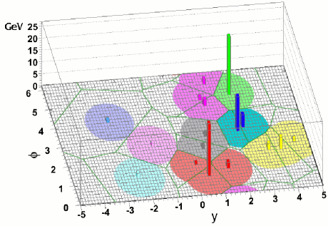
The Voronoi construction of the $k_{t}$-algorithm passive area is illustrated in fig. 2.1. One sees both the Voronoi cells and how their intersection with circles of radius $R=1$ gives the area of the particles making up those jets.

Note that it is not possible to write passive areas for jet algorithms other than $k_{t}$ in the form Eq. (2.15). One can however introduce a new type of area for a generic algorithm, a Voronoi area, in the form

$$a_{\text{JA},R}^{{\cal V}}(J)=\sum_{p_{i}\in J}a_{R}^{{\cal V}}(p_{i})\,.$$ (2.18)

While for algorithms other than $k_{t}$ (for which, as we have seen, $a_{k_{t},R}(J)=a_{k_{t},R}^{{\cal V}}(J)$), this area is not in general related to the clustering of any specific kind of background radiation, it can nevertheless be a useful tool, because its numerical evaluation is efficient [47, 17] and as we shall discuss later when we discuss analytic properties of jet areas (section 5.1), for dense events its value coincides with both passive and active area definitions.

2.3.3 Active Area, catchment area for pileup subtraction

To define an active area, as for the passive area, we start with an event composed of a set of particles $\{p_{i}\}$ which are clustered into a set of jets $\{J_{i}\}$ by some infrared-safe jet algorithm. However, instead of adding a single soft ghost particle, we now add a dense coverage of ghost particles, $\{g_{i}\}$, randomly distributed in rapidity and azimuth, and each with an infinitesimal transverse momentum. The clustering is then repeated including the set of particles plus ghosts.

During the clustering the ghosts may cluster both with each other and with the hard particles. This more ‘active’ participation in the clustering is the origin of the name that we give to the area defined below. It contrasts with the passive area definition (section 2.3.1) in which the single ghost acted more as a passive spectator.

Because of the infrared safety of any proper jet algorithm, even the addition of many ghosts does not change the momenta of the final jets $\{J_{i}\}$. However these jets do contain extra particles, ghosts, and we use the number of ghosts in a jet as a measure of its area. Specifically, if the number of ghosts per unit area (on the rapidity–azimuth cylinder) is $\nu_{g}$ and ${\cal N}_{g}(J)$ is the number of ghosts contained in jet $J$, then the (scalar) active area of a jet, given the specific set of ghosts $\{g_{i}\}$ is

$$\boxed{A(J\,|\,{\{g_{i}\}})=\frac{{\cal N}_{g}(J)}{\nu_{g}}}\,.$$ (2.19)

Figure 2.2: Active area for the same event as in figure 2.1, once again clustered with the $k_{t}$ algorithm (left) and the anti-$k_{t}$ algorithm (right) both using $R=1$. Only the areas of the hard jets have been shaded — the pure ‘ghost’ jets are not shown.

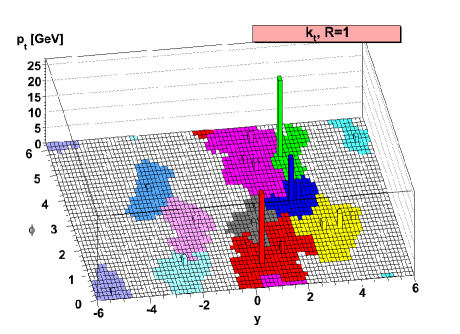
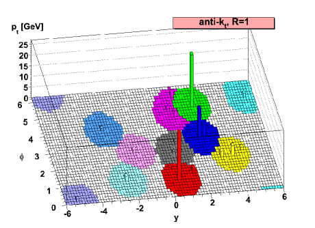
An example of jet areas obtained in this way is shown in figure 2.2. One notes that the boundaries of the jets obtained with the $k_{t}$ algorithm (the left plot) are rather ragged. Clustering with a different set of ghosts would lead to different boundaries. This is because the ghosts can cluster among themselves to form macroscopic subjets, whose outlines inevitably depend on the specific set of initial ghosts, and these then subsequently cluster with true event particles. This can happen for any density of ghosts, and thus the jet boundaries tend to be sensitive to the randomness of the initial sets of ghosts. This is true for most jet algorithms. One noticeable exception is the case of the anti-$k_{t}$ algorithm (right plot in Fig. 2.2). In that case, ghosts will cluster with the particles in the event before they cluster among themselves. The boundaries of the jets are thus defined by the structure of the event, (almost) independently of the initial set of ghosts. In particular, the hard jets will be circular, as seen in Fig. 2.2.

This randomness propagates through to the number of ghosts clustered within a given jet, even in the limit $\nu_{g}\to\infty$, resulting in a different area each time. To obtain a unique answer for active area of a given jet one must therefore average over many sets of ghosts, in addition to taking the limit of infinite ghost density,

$$\boxed{A(J)=\lim_{\nu_{g}\to\infty}\left\langle A(J\,|\,{\{g_{i}\}})\right\rangle_{g}}\,.$$ (2.20)

Note that as one takes $\nu_{g}\to\infty$, the ghost transverse momentum density, $\nu_{g}\langle g_{t}\rangle$, is to be kept infinitesimal. For most practical applications, including the case of pileup mitigation, one has many particles in the event and the boundaries of the jets are well determined by the particles in the event leaving only very little dependence on actual set of ghosts. In practice we can therefore use a unique set of ghost to determine the active area which is far less time-consuming than having to average over many sets. This is what we have done throughout this review. Note however that for low-multiplicity events the active area can fluctuate significantly between different sets of ghosts (see for example Fig. 5.4 which shows the distribution of active areas for different sets of ghosts, for events with a single particle or for jets made purely of ghosts in the absence of any hard particles).

The active area bears a close resemblance to the average susceptibility of the jet to a high density of soft radiation like pileup, since the many soft particles will cluster between each other and into jets much in the same way as will the ghosts. In that sense, the “area of the jet”, $A_{\rm jet}$, referred to in our introductory description of pileup effects (see Section 2.1), has to be seen as an active area.

A feature that arises when adding many ghosts to an event is that some of the final jets contain nothing but ghost particles. They did not appear in the original list of $\{J_{i}\}$ and we refer to them as pure ghost jets. These pure ghost jets (not shown in fig. 2.2), fill all of the ‘empty’ area, at least in jet algorithms for which all particles are clustered into jets. They will be similar to the jets formed from purely soft radiation in events with minimum-bias pileup, and so are interesting to study in their own right and will play a crucial role in the area–median subtraction method.

In analogy with the 4-vector passive area, we can define a 4-vector version of the active area. It is given by

$$A_{\mu}(J\,|\,{\{g_{i}\}})=\frac{1}{\nu_{g}\langle g_{t}\rangle}\sum_{g_{i}\in J}g_{\mu i}\,,\qquad\quad A_{\mu}(J)=\lim_{\nu_{g}\to\infty}\left\langle A_{\mu}(J\,|\,{\{g_{i}\}})\right\rangle_{g}\,.$$ (2.21)

The sum of the $g_{\mu i}$ is to be understood as carried out in the same recombination scheme as used in the jet clustering.

One may also define the standard deviation $\Sigma(J)$ of the distribution of a jet’s active area across many ghost ensembles,

$$\Sigma^{2}(J)=\lim_{\nu_{g}\to\infty}\left\langle A^{2}(J\,|\,{\{g_{i}\}})\right\rangle_{g}-A^{2}(J)\,.$$ (2.22)

This provides a measure of the variability of a given jet’s contamination from (say) pileup and is closely connected with the momentum resolution that can be obtained with a given jet algorithm.

2.4 Area–median pileup subtraction

2.4.1 Basic recipe for pileup subtraction

Now that we have a well-defined concept of the area of a jet in our toolkit, we can finally introduce the area–median approach.

Coming back to our original discussion of the pileup effects, we have noticed that pileup introduces an average bias appearing as a shift of the jet transverse momentum, as well as a smearing of its resolution. We aim at a method that would remove the $p_{t}$ shift on average, i.e. be unbiased on average, and limit the residual resolution degradation effects to a minimum. Looking at equations (2.1), (2.4) and (2.5), it is preferable to apply a correction that avoids making too many averages which would each time result in additional contributions to the resolution degradation.

The main idea of the area–median pileup subtraction technique is to subtract from the jet transverse momentum $p_{t,\rm full}$ its average shift $\rho A_{\rm jet}$ in (2.1). This requires two ingredients: the calculation of the jet area, which we already have under the form of the active area introduced in the previous Section, and a method to obtain an estimate of $\rho$, $\rho_{\rm est}$.

The estimation of the average pileup activity in an event is based on the observation that, if we break an event into patches, most of the patches will not contain particles from the hard jets and for those patches $p_{t,\rm patch}/A_{\rm patch}$ is, on average, a good estimate of $\rho$. Averaging the $p_{t,\rm patch}/A_{\rm patch}$ over all the patches would however not give a good estimate of $\rho$ since it will be strongly biased by the few patches containing particles from the hard jets. In practice, it was found [5] that the median of $p_{t,\rm patch}/A_{\rm patch}$ provides a good estimate of $\rho$, not significantly affected by the “outlying” patches containing particles from the hard jets.

In the end, the area–median subtraction method works as follows:

• Find an estimate of $\rho$: 1. Break the event into patches of similar area. Typically, one can break the event into grid cells in the $y-\phi$ plane (“grid–median” estimator). Alternatively, one can use $k_{t}$ [45, 46] or Cambridge/Aachen [49, 50] jets obtained with a jet radius potentially different from the one used to cluster the physical jets (“jet–median” estimator). 2. Compute the momentum and area of each patch. When patches are grid cells, one could use the scalar $p_{t}$ and scalar, geometric, area, while for jet patches, one would rather use their 4-vector $p_{t}$ together with the transverse component of the 4-vector active area. 3. The estimate of $\rho$ is given by $$\rho_{\rm est}=\underset{i\in\rm patches}{{\rm median}}\left\{\frac{p_{t,i}}{A_{i}}\right\}$$ (2.23) where the empty cells or the pure-ghost jets are included in the calculation. • Subtract pileup from physical jets: 1. cluster the jets with your favourite jet definition, computing their active area 2. correct their 4-momentum using $$p_{\mu}^{\rm(sub)}=p_{\mu}-\rho_{\rm est}A_{{\rm jet},\mu}.$$ (2.24)

Modulo possible offsets in the estimation of $\rho$ (see Section 5.2 for details), the area–median method would subtract from each jet its $\rho A_{\rm jet}$ contamination, leaving a jet with, on average, an unbiased transverse momentum, with a $p_{t}$ resolution degradation given by $\sigma\sqrt{A_{\rm jet}}$. There could also be an additional bias and resolution degradation coming from back-reaction although, apart from the resolution degradation at large $p_{t}$, this can safely be ignored when subtracting pileup from anti-$k_{t}$ jets which covers the vast majority of the applications. Overall, we therefore expect the area–median approach to provide jets with better resolution than alternative unbiased approaches like subtracting an average pileup contamination per pileup vertex or an overall average pileup contamination, since these would result in additional sources of resolution degradation. The key element behind this is the fact that the pileup activity, $\rho$, is estimated fully dynamically on an event-by-event basis with the jet area computed individually for each jet. The left-over resolution degradation due to pileup fluctuations are of the order of the much-smaller $\sigma$.

When implementing this procedure in a practical context, several technical details have to be fixed like the rapidity coverage for particles and ghosts or the size of the patches. We will come back to these in Section 2.8. Here we rather discuss the physics behind the area–median approach and carry on with extensions in the next Sections.

The area–median method would work basically with any jet algorithm giving well-defined active jet areas. Apart from some fancy grooming techniques, this mostly means that it works with any infrared-safe jet algorithm.

A potentially non-trivial point is why empty patches (or pure-ghost jets) have to be included in the calculation of the median. In an event with a large pileup activity, where the whole event is densely populated, this would make no difference. However, when the event becomes sparse, e.g. when applying our procedure to parton-level Monte-Carlo simulations or with events with no or little pileup activity, most of the non-empty patches would be made of hard jets. Including empty patches would then avoid having $\rho_{\rm est}$ set to the scale of the hard jets.

Note that, conceptually, one can view the area–median pileup subtraction method as part of the jet definition. In that viewpoint, jets are defined by applying the anti-$k_{t}$ algorithm with a given radius (or any other jet definition one wishes to use) and subtracting the result using the area–median method. It is the combination of these two steps which can be seen as a jet definition.

Furthermore, the Underlying Event produced in proton-proton collisions also corresponds to a largely uniform energy deposit. It will therefore also be subtracted by the area–median method. We will discuss this in more details in Section 3.2.6.

2.4.2 Positional dependence

So far, we have assumed that, apart from small up and down fluctuations of order $\sigma$, the pileup energy deposit is uniform in rapidity and azimuthal angle. We know however that this is not true in practice. The most striking example is that the energy deposit in a minimum bias collision is, on average, larger in central rapidities than in the forward regions, translating into an average pileup transverse momentum $\rho$ larger in the central region than at forward rapidities. Another example is the case of heavy-ion collisions where flow [19, 20, 21, 22, 23, 24, 25, 26, 27] would also generate a non-trivial $\phi$ dependence, mostly dominated by elliptic flow and its $\cos(2\phi)$ dependence. In both cases, the background density $\rho$ will vary smoothly across an event.

From the perspective of pileup subtraction, this means that we have to deal with a situation where $\rho$ depends on the position of the jet $j$ that one wants to subtract. The area–median approach proposes two methods to handle the positional dependence of $\rho$, both based on adaptations of Eq. (2.23).

Figure 2.3: Typical local ranges that can be used for the estimation of the positional-dependent pileup density $\rho(j)$, compared to a global range (left).

Local range.

The first method is to estimate $\rho$ only from the patches which are in the local vicinity of the jet one wishes to subtract:

$$\boxed{\rho_{{\rm est},{\cal R}}(j)=\underset{i\in{\rm patches}\in{\cal R}(j)}{\rm median}\left\{\frac{p_{t,i}}{A_{i}}\right\}}\,,$$ (2.25)

where ${\cal R}(j)$ denotes a local range around jet $j$. Typical choices for ${\cal R}(j)$ are the following:

• the Strip range, ${\cal S}_{\Delta}(j)$, includes the jets $j^{\prime}$ satisfying $|y_{j^{\prime}}-y_{j}|<\Delta$,

• the Circular range, ${\cal C}_{\Delta}(j)$, includes the jets $j^{\prime}$ satisfying $\sqrt{(y_{j^{\prime}}\!-\!y_{j})^{2}+(\phi_{j^{\prime}}\!-\!\phi_{j})^{2}}<\Delta$,

• the Doughnut range, ${\cal D}_{\delta,\Delta}(j)$, includes the jets $j^{\prime}$ satisfying $\delta<\sqrt{(y_{j^{\prime}}\!-\!y_{j})^{2}+(\phi_{j^{\prime}}\!-\!\phi_{j})^{2}}<\Delta$.

These three options are depicted in Figure 2.3.

Note that, when using a local range, a compromise has to be found between taking it large enough so that it contains enough patches for the estimation of the median to be reliable, and not too large to capture the positional dependence of $\rho$. Based on analytic estimates discussed in Section 5.2, we can show that for jets of radius $R$, if we want the uncertainty on the determination of $\rho$ to contribute at most for a fraction $\epsilon$ of the natural pileup fluctuations $\sigma\sqrt{A_{\rm jet}}$, the range needs to cover at least an area $A_{{\cal{R}}}$ such that

$$A_{{\cal{R}}}\gtrsim\frac{\pi^{2}R^{2}}{4\epsilon}.$$ (2.26)

For $\epsilon=0.1$ and $R=0.4$, this gives $A_{{\cal{R}}}\gtrsim 4$. We will discuss this in more details in our Monte Carlo studies of heavy-ion collisions in Chapter 4.

Rescaling.

The alternative approach is to correct for the positional dependence before taking the median. In practice, if $f(j)$ captures the positional dependence of the pileup energy deposit as a function of the position $j$ (arbitrarily normalised), we can use this as a rescaling function and compute the background density at the position $j$ using

$$\boxed{\rho_{{\rm est},f}(j)=f(j)\,\underset{i\in{\rm patches}}{\rm median}\left\{\frac{p_{t,i}}{A_{i}\,f(i)}\right\}}\,,$$ (2.27)

where $f(i)$ is the positional dependence computed at the position of “patch $i$”.

Compared to the local-range approach, this requires the rescaling function $f$ to be computed before using Eq. (2.27). In the situation where this is used to correct for the smooth rapidity dependence of pileup, this function can be taken from an average over minimum bias events. For elliptic flow in heavy-ion collisions, $f(j)$ can be parametrised as a function of the event plane and $v_{2}$ determined event-by-event.

We shall discuss in more details these local estimates later, when we validate the area–median subtraction using Monte-Carlo simulations (Section 3.2). We shall also discuss the local range approach when we discuss heavy-ion collisions (Chapter 4).

2.4.3 Particle masses

In order to obtain a full pileup subtraction of the jet 4-momentum, there is a last ingredient that needs to be discussed: the effect of particle masses.

To see this, let us go back to the basic area–median method described in Section 2.4.1 and to equation (2.24) in particular. The 4-vector jet area is nothing but a 4-vector sum over the ghosts inside the jets (see e.g. Eq. (2.21)). The main formula (2.24) can then be seen as subtracting from the jet 4-vector, $j^{\mu}$, an amount $a\rho\,g^{\mu}$ for each ghost in the jet. In this expression, $a=1/\nu$ is the fundamental area carried by each ghost and $\rho$ is the appropriate conversion factor to correct for the jet transverse momentum. In other words, (2.24) makes a parallel between the pileup particles contaminating the jet and the ghosts used to calculate the jet area, using the latter to subtract the former through an estimate of the proportionality constant $\rho$.

This analogy between the pileup particles and the ghosts is however no longer exact when pileup particles become massive since the ghosts are massless. On top of its rapidity and azimuth, a generic 4-vector has two additional degrees of freedom: its transverse momentum $p_{t}$ and its transverse mass $m_{t}=\sqrt{p_{t}^{2}+m^{2}}$, with $m$ its mass. Since $\rho$ is determined from the transverse-momentum component of the patches, subtracted a 4-vector proportional to a jet area made of massless ghosts will result in a small mismatch for the components of the jet sensitive to the mass of the particles.

To put this discussion on a more formal ground, let us take an infinitesimal patch of the event of size $\delta y\times\delta\phi$. The 4-vector corresponding to a uniform pileup deposit in that patch will take the generic form

$$(p_{x},p_{y},p_{z},E)\equiv(\rho\cos(\phi),\rho\sin(\phi),(\rho+\rho_{m})\sinh(y),(\rho+\rho_{m})\cosh(y))\,\delta y\,\delta\phi\,$$ (2.28)

where we have used the fact that $\rho$ is defined as the pileup transverse momentum per unit area — estimated using Eq. (2.23) — and the longitudinal components, $p_{z}$ and $E$, can receive an extra contribution coming from the mass of the pileup particle. The new term $\rho_{m}$ is an extra pileup contamination that comes from the fact that the transverse mass is larger than the transverse momentum for massive particles. A uniform pileup deposit is therefore characterised by 2 numbers: $\rho$ and $\rho_{m}$.

The correction for the $\rho$ contamination can be carried over using the method already presented in Section 2.4.1 and correcting from the new $\rho_{m}$ term can be straightforwardly done following the same logic. We first estimate $\rho_{m}$ using a median approach:

$$\boxed{\rho_{m,\rm est}=\underset{i\in\rm patches}{{\rm median}}\left\{\frac{m_{\delta,i}}{A_{i}}\right\},}$$ (2.29)

with $m_{\delta,{\rm patch}}=\sum_{i\in{\rm patch}}\sqrt{p_{t,i}^{2}+m_{i}^{2}}-p_{t,i}$, where the sum runs over all the particles in the patch. We then correct the jet 4-vector using

$$\boxed{p_{\mu}^{\rm(sub)}=p_{\mu}-(\rho_{\rm est}A_{{\rm jet},x},\>\rho_{\rm est}A_{{\rm jet},y},\>(\rho_{\rm est}+\rho_{m,\rm est})A_{{\rm jet},z},\>(\rho_{\rm est}+\rho_{m,\rm est})A_{{\rm jet},E}).}$$ (2.30)

These expressions can easily be extended to include positional dependence either using local ranges or using a rescaling function. In the second case, note that for all the applications we have seen, a common rescaling function for $\rho$ and $\rho_{m}$ is good enough (see also Section 3.1).

2.4.4 Safe subtraction and positivity constraints

There are a few cases where the area–median subtraction formula could lead to unphysical jets.

The first one is when $\rho A$ is larger than the (unsubtracted) $p_{t}$ of the jet. This could typically happen for low-$p_{t}$ jets sitting on a downwards pileup fluctuation and would lead to jets with “negative” $p_{t}$ after subtraction. In this case, the most reasonable prescription is usually to set the subtracted jet to a vanishing 4-momentum.

The second case would be a jet with a positive transverse momentum but a negative squared mass. In this case, a good prescription is to keep the transverse momentum and azimuth of the jet obtained after subtraction of the $\rho$ contamination, take the rapidity of the original jet and set its mass to 0.

We will explicitly refer to these prescriptions as “safe” subtraction and discuss them later in our Monte Carlo tests (see Chapter 11).

2.4.5 Extension to Charged-Hadron Subtracted (CHS) events

In several experimental contexts, it is possible to associate charged tracks either to the leading vertex or to a pileup interaction. In that context, one builds a Charged-Hadron-Subtracted (CHS) event where one subtracts the tracks associated to pileup interactions keeping only the tracks associated with the leading vertex and the neutral particles (or energy deposits) coming either from the leading vertex or from pileup. Optionally, the charged tracks associated with a pileup vertex can be retained as ghosts, i.e. with their momentum scaled down by a large factor, in order to retain information about their presence in the original event. Modulo experimental complications, this considerably reduces the pileup contamination (both the average shift and the dispersion), since charged tracks account for about a fraction $f\approx 062$ of the pileup energy deposit.

The area–median method can be straightforwardly applied to CHS events, with the pileup properties estimated either on the full CHS event or only on their neutral component. One should expect a reduction of the average pileup contamination by a factor $1/(1-f)\approx 2.6$ and of the resolution smearing by a factor $1/\sqrt{1-f}\approx 1.6$. Although results from Chapter 3 directly extend to CHS events, we will discuss this at length in Chapter 11 where we compare the area–median approach to alternative methods that make use of charged track information.

2.5 Jet shapes

So far, we have introduced the area–median method for subtracting pileup contamination from the jet 4-momentum. It is now natural to ask if the method can be extended to more general properties of the jets. In this Section, we show that it is possible to obtain a generic area–median subtraction method for jet shapes, i.e. infrared-and-collinear safe functions of the jet constituents.

Let us therefore consider a generic infrared-and-collinear-safe function $v_{\rm jet}(\{p_{i}\})$ of the jet constituents $\{p_{i}\}$, including a uniform pileup contamination characterised by the scales $\rho$ and $\rho_{m}$. We also include in these constituents a set of ghosts each carrying an area $A_{g}=1/\nu$ in the $y-\phi$ plane and to which we associate an infinitesimal transverse momentum $p_{t,g}$ and a (new) infinitesimal transverse mass $m_{t,g}=p_{t,g}+m_{\delta,g}$ with $m_{\delta,g}=\sqrt{p_{t.g}^{2}+m_{g}^{2}}-p_{t,g}$. As discussed in Section 2.4.3, these ghosts mimic the effect of a uniform pileup deposit and the ghost scales $p_{t,g}$ and $m_{\delta,g}$ correspond to the pileup densities $\rho$ and $\rho_{m}$.

For any given jet we can then consider the derivatives of the jet shape w.r.t. to the ghost transverse scales $p_{t,g}$ and $m_{\delta,g}$,

$$v_{\rm jet}^{(m,n)}=A_{g}^{m+n}\partial_{p_{t,g}}^{m}\partial_{m_{\delta,g}}^{n}v_{\rm jet}(\{p_{i}\}).$$ (2.31)

In a sense, these derivatives probe the susceptibilities of the shape to the $\rho$ and $\rho_{m}$ components of pileup and can be used to correct the shape $v$ by extrapolating its value down to zero pileup:

$$v^{\rm(sub)} =\sum_{m=0}^{\infty}\frac{1}{m!}\sum_{n=0}^{\infty}\frac{1}{n!}(-)^{m+n}\rho^{m}\rho_{m}^{n}v_{\rm jet}^{(m,n)}$$ (2.32)

$$\approx v_{\rm jet}-\rho v_{\rm jet}^{(1,0)}-\rho_{m}v_{\rm jet}^{(0,1)}+\frac{1}{2}\rho^{2}v_{\rm jet}^{(2,0)}+\rho\rho_{m}v_{\rm jet}^{(1,1)}+\frac{1}{2}\rho_{m}^{2}v_{\rm jet}^{(0,2)}+\dots,$$ (2.33)

where the second line is expanded to second order in the pileup properties. This second-order subtraction is the main formula we shall use to subtract jet shapes.

It is illustrative to consider two specific examples of this formula: the jet transverse momentum and the jet mass squared. For the jet transverse momentum, the uniform pileup distribution will shift the original hard transverse momentum $p_{t,\rm hard}$ (without pileup), by an amount $A_{\perp}\rho$, with $A_{\perp}$ the transverse momentum component of the jet area 4-vector. On top of that, the ghosts will add a contribution $p_{t,g}A_{\perp}/A_{g}$ to the total $p_{t}$, giving successively

$$p_{t} =p_{t,\rm hard}+(\rho+p_{t,g}/A_{g})A_{\perp},$$ (2.34)

$$p_{t}^{(1,0)} =A_{\perp},$$ (2.35)

with all other derivatives vanishing, and finally,

$$p_{t}^{\rm(sub)}=p_{t}-\rho p_{t}^{(1,0)}=p_{t}-\rho A_{\perp}=p_{t,\rm hard}+p_{t,g}A_{\perp}/A_{g}=p_{t,\rm hard}$$ (2.36)

where, for the last equality, we have dropped the negligible contribution coming from the infinitesimal $p_{t}$ of the ghosts. This simple exercise shows that (2.33) reduces to the expression $p_{t}^{\rm(sub)}=p_{t}-\rho A_{\perp}$ at the core of the area–median subtraction. It also provides an interesting interpretation of the “jet area” as the susceptibility of the jet transverse momentum to variations of the background density $\rho$.

Albeit a bit more involved technically, the case of the squared jet mass flows similarly. Let us consider a hard jet of transverse momentum $p_{t,\rm hard}$ and mass $m_{\rm hard}$ with additional uniform pileup contamination and ghosts. We already know that the hard jet transverse momentum is shifted by $(\rho+p_{t,g}/A_{g})A_{\perp}$ and, in a similar way, the jet transverse mass will be shifted by $(\rho+p_{t,g}/A_{g})A_{\perp}+(\rho_{m}+m_{\delta,g}/A_{g})A_{\rm jet}$, where we have separated the contribution from the transverse momentum and the one from the particle masses. This gives

$$m^{2} =\left[\sqrt{p_{t,\rm hard}^{2}+m_{\rm hard}^{2}}+(\rho+p_{t,g}/A_{g})A_{\perp}+(\rho_{m}+m_{\delta,g}/A_{g})A_{\rm jet}\right]^{2}-\left[p_{t,\rm hard}+(\rho+p_{t,g}/A_{g})A_{\perp}\right]^{2},$$

$$m^{2(1,0)} =2A_{\perp}\left[\sqrt{p_{t,\rm hard}^{2}+m_{\rm hard}^{2}}-p_{t,\rm hard}+(\rho_{m}+m_{\delta,g}/A_{g})A_{\rm jet}\right],$$

$$m^{2(0,1)} =2A_{\rm jet}\left[\sqrt{p_{t,\rm hard}^{2}+m_{\rm hard}^{2}}+(\rho+p_{t,g}/A_{g})A_{\perp}+(\rho_{m}+m_{\delta,g}/A_{g})A_{\rm jet}\right],$$

$$m^{2(2,0)} =0,$$

$$m^{2(1,1)} =2A_{\perp}A_{\rm jet},$$

$$m^{2(0,2)} =2A_{\rm jet}^{2},$$ (2.37)

with higher derivatives vanishing. Substituting this in (2.33), and neglecting the infinitesimal ghosts, we find after easy manipulations

$$m^{2\rm(sub)}=m_{\rm hard}^{2}.$$ (2.38)

Note that, in order to recover exactly the hard jet without pileup contamination, it is important to apply the subtraction procedure to the jet mass squared. This is mostly because, as can be seen from (2.5), the squared mass $m^{2}$ is explicitly quadratic in $p_{t,g}$ and $m_{\delta,g}$. If we were to apply the subtraction formula to the jet mass, the extra square root would translate in non-vanishing higher derivatives and subtracting pileup contamination up to second-order would leave some (parametrically small) residual corrections (proportional to $\rho^{3}/m^{2}$ at large $p_{t}$).

These examples show not too surprisingly that our second-order expansion would work better if the quadratic approximation works fine. As we shall see in practice in Monte Carlo simulations, there are some notorious cases where this approximation tends to break. One typical example is when a shape has an endpoint and the effect of pileup is to bring the value of the shape close to that endpoint.

In some situations, it is however possible to work around these limitations by splitting the shape into components and subtracting these components individually before reconstructing the final subtracted shape from the subtracted components. The case of the $N$-subjettiness ratio $\tau_{21}=\tau_{2}/\tau_{1}$ illustrates this very well: while $\tau_{21}$ itself has a complicated dependence on the pileup density, (unnormalised) $\tau_{1}$ and $\tau_{2}$ are linear in $\rho$. We should therefore apply the subtraction procedure to $\tau_{1}$ and $\tau_{2}$ and reconstruct the subtracted value of $\tau_{21}$ from those. The only delicate point here is to properly handle the situation where the subtracted value of $\tau_{1}$ becomes 0 or negative, e.g. by setting the subtracted value of $\tau_{21}$ to 0.

Generally speaking, subtracting the shape as a single entity or breaking the shape in components and subtracting these components individually tend to be affected by different effects. Depending on the specific details of the shape and how it is used in a given analysis, one method or the other would give slightly better results (e.g. for $\tau_{21}$, the subtraction as a single entity works slightly better at smaller $\tau_{21}$ but the splitting into components is marginally preferred at larger $\tau_{21}$). For simplicity, we will apply the subtraction to the shape as a single entity in our later tests in Section 3.3.

Finally, let us note that it is possible to rewrite (2.33) in terms of a single variable. We can for example introduce a variable $x_{g}$ such that $p_{t,g}=x_{g}$ and $m_{\delta,g}=\rho_{m}/\rho x_{g}$ and define

$$\boxed{v_{\rm jet}^{[k]}=A_{g}^{k}\partial_{x_{g}}^{k}v_{\rm jet}(\{p_{i}\}).}$$ (2.39)

The subtraction formula then takes the simpler form

$$\boxed{v^{\rm(sub)}=\sum_{k=0}^{\infty}\frac{1}{k!}(-)^{k}\rho^{k}v_{\rm jet}^{[k]}\approx v_{\rm jet}-\rho v_{\rm jet}^{[1]}+\frac{1}{2}\rho^{2}v_{\rm jet}^{[2]}+\dots.}$$ (2.40)

2.6 Jet fragmentation function

At this stage, we have seen that the area–median pileup subtraction method can be applied to all infrared and collinear safe jet observables. In this section, we shall add to that list yet another observable, the jet fragmentation function, which is collinear unsafe.

Part of the idea behind the area–median subtraction of the jet fragmentation function is to subtract its moments rather than the direct distribution. We provide a discussion of the different representations of a jet fragmentation function in Appendix B, including some additional physics motivations to consider the moments of the jet fragmentation function. Here we shall just recall the basic definitions.

Definition.

The jet fragmentation function (FF) is defined as the distribution $dN_{h}/dz$ of the momentum fraction

$$z=\frac{p_{t,h}}{\tilde{p}_{t}}$$ (2.41)

of all the hadrons $h$ in a jet. In the definition of $z$, $p_{t,h}$ is the transverse momentum of the hadron and $\tilde{p}_{t}$ is the scalar $p_{t}$ of the jet, defined as the scalar sum of the transverse momenta of the constituents of the jet, $\tilde{p}_{t}=\sum_{i\in{\rm jet}}p_{t,i}$. In future discussions it will also be interesting to define $\xi=\log(1/z)$. In practice, the distribution $dN_{h}/dz$ is usually binned in $z$ or $\xi$ and normalised to the number $N_{\rm jet}$ of jets in the sample.

Instead of applying the pileup subtraction directly to $dN_{h}/dz$, we will rather do it to its moments defined as

$$M_{N}=\frac{1}{N_{\rm jet}}\int_{0}^{1}dz\,z^{N}\,\frac{dN_{h}}{dz}=\frac{1}{N_{\rm jet}}\int_{0}^{\infty}d\xi\,e^{-N\xi}\,\frac{dN_{h}}{d\xi}.$$ (2.42)

In practice, one usually computes the $N$th moment for a single jet:

$$M_{N}^{\rm jet}=\frac{\sum_{i\in\rm jet}p_{t,i}^{N}}{\tilde{p}_{t}^{N}},$$ (2.43)

and average over the jet sample, $M_{N}=\langle M_{N}^{\rm jet}\rangle$.

Area–median subtraction.

We can use an adaptation of the area–median approach to directly subtract the moments $M_{N}$ of the fragmentation function.

The procedure to subtract the FF moments is quite similar to the main area–median approach. One first determines the expected background contribution per unit area to a given moment (or rather to its numerator in Eq. (2.43)):

$$\boxed{\rho_{N}=\mathop{\text{median}}_{\text{patches}}\left\{\frac{\sum_{i\in\text{patch}}p_{t,i}^{N}}{A_{\text{patch}}}\right\}\,.}$$ (2.44)

For example, for $N=0$ this will be the median particle multiplicity per unit area. The subtracted FF moment is then obtained by separately taking the numerator and denominator of Eq. (2.43), as measured in the full event, and respectively subtracting $\rho_{N}A$ and $\rho A$:

$$\boxed{M_{N}^{\text{sub}}=\frac{\sum_{i\in\text{jet}}p_{t,i}^{N}-\rho_{N}A}{(p_{t,\text{full}}-\rho A)^{N}}\,.}$$ (2.45)

Improved background-subtracted fragmentation function.

In Section 4.7, we will apply this subtraction method to FF measurements in heavy-ion collisions and observe that it is insufficient to fully correct the jet FF moments. We believe this can largely be attributed to background fluctuations and we describe below an improved subtraction method that corrects for the dominant fluctuation effects.

Background fluctuations mean that neither the jet’s $p_{t}$ nor the numerator of the FF moment are perfectly reconstructed for any given jet. When selecting jets above some $p_{t}$ threshold for a process with a steeply falling jet spectrum, it is favourable to select jets slightly below the $p_{t}$ threshold, but which have an upwards background fluctuation (cf. the discussion of Section 2.2). One consequence of this is that the denominator in Eq. (2.45) tends to be larger than the actual jet $p_{t}$. The larger the value of $N$, the greater the impact of this effect. One can also understand it as resulting in an underestimate of the $z$ fraction, leading to the FF being spuriously shifted to lower $z$. Such an effect is already well known: CMS [52], for example, when comparing with $pp$ FFs, explicitly applies a correction to the $pp$ FFs to account for the smearing of the denominator of the $z$ variable that is expected when the jet’s momentum is reconstructed in a HI environment. ATLAS [53] carries out an unfolding to account for this. Implementing an additional correction for the dominant background fluctuations effects will reduce the size of the final unfolding corrections and hopefully of the associated uncertainties. We note that a key argument here is that the dominant fluctuation effects are local in moment space $N$, therefore avoiding more complex (unfolding) corrections in $z$ space which is additionally affected by bin-migration effects.

A second consequence of fluctuations affects mostly the low-$z$, or low-$N$ region of the FF: the upwards fluctuations of the background $p_{t}$ that cause a jet to pass the $p_{t}$ cut even when it is below threshold also tend to be associated with upwards fluctuations of the multiplicity of soft background particles. It is this effect that causes the FF to be overestimated for low values of $N$.

One way of verifying the above interpretation is to consider $\gamma+$jet events, selecting events based on the photon $p_{t}$ and normalising the fragmentation function $z$ also to the photon $p_{t}$. In this case, the background-induced fluctuations of the jet’s reconstructed $p_{t}$ are of no relevance, and in explicit simulations, we have found that plain subtraction is already quite effective.

For the dijet case, in the limit where the background fluctuations are reasonably small compared to the transverse momentum of the jet, it is possible to devise a simple correction in moment space for both kinds of fluctuation-induced bias. In order to do so, we start by rewriting the subtracted moments of the jet FF in Eq. (2.45) as

$$M_{N}^{\text{sub}}=\frac{\sum_{i}p_{t,i}^{N}-\rho_{N}A}{(p_{t,\text{full}}-\rho A)^{N}}\equiv\frac{S_{N}}{S_{1}^{N}}$$ (2.46)

where we have introduced the shorthands $S_{N}$ for the subtracted numerator and $S_{1}$ for $p^{\text{sub}}_{t,\text{full}}$, as defined by the area–median subtraction, Eq. (2.24). Given our assumption that background fluctuations are moderate, we can locally approximate the hard jet cross-section by an exponential (as already done in Section 2.2)

$$H(p_{t})\equiv\frac{d\sigma}{dp_{t}}=\frac{\sigma_{0}}{\kappa}\,{\rm exp}(-p_{t}/\kappa)\,.$$ (2.47)

We then take a Gaussian approximation for the spectrum of background transverse-momentum fluctuations from one jet to the next. Denoting the fluctuation by $q_{t}$, the distribution of $q_{t}$ is then

$$B(q_{t})\equiv\frac{dP}{dq_{t}}=\frac{1}{\sqrt{2\pi A}\sigma}\,\exp\left(-\frac{q_{t}^{2}}{2\sigma^{2}A}\right),$$ (2.48)

where $\sigma$ is a parameter that describes the size of fluctuations from one patch of area $1$ to another. For patches of area $A$, the variance of the $q_{t}$ across the patches is $\sigma^{2}A$.

We further introduce the variable $Q_{N}$ to denote the difference between the actual background contribution to $S_{N}$ in a specific jet and the expected contribution, $\rho_{N}A$, i.e.

$$Q_{N}=\left(\sum_{i\,\in\,\text{jet\,(bkgd)}}k_{t,i}^{N}\right)-\rho_{N}A\,,$$ (2.49)

where the sum runs just over the background constituents $k_{t,i}$ of the jet. By construction, $Q_{1}=q_{t}$. In practice $Q_{N}$ cannot be determined for a single jet, since we don’t know which particles are the background ones, but its statistical properties can be determined by looking at many jets, and we denote the standard deviation of its fluctuations from one patch of area $1$ to another by $\sigma_{N}$, in direct analogy to $\sigma$. The fluctuations of $Q_{N}$ are not independent of the fluctuations $q_{t}$ of the background’s transverse momentum: there is a correlation coefficient $r_{N}$ between them, defined as

$$r_{N}=\frac{\mathrm{Cov}(q_{t},Q_{N})}{\sqrt{\mathrm{Var}(q_{t})\mathrm{Var}(Q_{N})}}\,,$$ (2.50)

where $\mathrm{Var}(X)$ is the variance of the variable $X$ and $\mathrm{Cov}(X,Y)$ the covariance of $X$ and $Y$. Using the fact that $\mathrm{Var}(q_{t})=\sigma^{2}A$, $\mathrm{Var}(Q_{N})=\sigma_{N}^{2}A$, we have that the average value for $Q_{N}$ as a function of $q_{t}$ is

$$\langle Q_{N}\rangle(q_{t})=\frac{\mathrm{Cov}(q_{t},Q_{N})}{\mathrm{Var}(q_{t})}q_{t}=r_{N}\frac{\sigma_{N}}{\sigma}q_{t}\,.$$ (2.51)

With these ingredients we can now correct for the fluctuation effects as follows. If we measure a certain value $S_{N}$ in a jet, then as a function of the $q_{t}$ fluctuation, the expected true hard contribution to it is

$$S_{N}^{\text{hard}}=S_{N}-\langle Q_{N}\rangle(q_{t})=S_{N}-r_{N}\frac{\sigma_{N}}{\sigma}q_{t}\,,$$ (2.52)

where we have averaged over possible $Q_{N}$ values, given the $q_{t}$ fluctuation. To obtain our estimate for $M_{N}^{\text{hard}}$, this should be normalised by the $N^{\text{th}}$ power of the true hard $p_{t}$ of the jet, $(S_{1}-q_{t})^{N}$:

$$M_{N}^{\text{hard}}=\frac{S_{N}^{\text{hard}}}{(S_{1}-q_{t})^{N}}=\frac{S_{N}}{S_{1}^{N}}+N\frac{S_{N}q_{t}}{S_{1}^{N+1}}-r_{N}\frac{\sigma_{N}q_{t}}{\sigma S_{1}^{N}}+{\cal O}\left(q_{t}^{2}\right)\,.$$ (2.53)

One subtlety here is that this is an estimate for $M_{N}^{\text{hard}}$ in hard jets with true $p_{t}=S_{1}-q_{t}$. However because $M_{N}$ is a slowly varying function of $p_{t}$, by taking the result as contributing to $M_{N}^{\text{hard}}(S_{1})$ rather than $M_{N}^{\text{hard}}(S_{1}-q_{t})$ we make only a small mistake, of the same order as other terms that we shall neglect.

Following Eq. (2.10), the average fluctuation $q_{t}$ for a given reconstructed $S_{1}$ is

$$\langle q_{t}\rangle=\frac{\sigma^{2}A}{\kappa},$$ (2.54)

therefore, retaining the terms linear in $q_{t}$ in Eq. (2.53) and averaging now over possible $q_{t}$ values, leads to the following prescription for an “improved” subtracted $M_{N}(S_{1})$, corrected for fluctuations effects up to first order in $q_{t}/S_{1}$:

$$\boxed{M_{N}^{\text{sub,imp}}=M_{N}^{\text{sub}}\times\left(1+N\frac{\sigma^{2}A}{S_{1}\kappa}\right)-r_{N}\frac{\sigma\sigma_{N}A}{\kappa S_{1}^{N}}\,.}$$ (2.55)

This is simpler than the corresponding correction would be directly in $z$ space, in particular because in $z$ space the correction to one bin of the fragmentation function depends in a non-trivial way on the contents of nearby bins. One can think of the advantages of moment space as being that the correction to a given $N$ value does not depend on $M_{N}$ at all other values of $N$, and that it is straightforward to account for correlations between fluctuations in the jet-$p_{t}$ and in the moments.

Note that in a real experimental context, calorimeter fluctuations of the reconstructed jet and background $p_{t}$’s would have an effect akin to increasing $\sigma$ and decreasing the correlation coefficient $r_{N}$. The in-situ methods that we use for the determination of $\sigma$, $\sigma_{N}$ and $r_{N}$ would automatically take this into account. Noise-reduction methods in the reconstruction of the jet $p_{t}$, as used by CMS [54], would have the effect of reducing $\sigma$ (and probably also $r_{N}$). However noise reduction is likely to complicate the meaningful determination of $r_{N}$, since it acts differently on pure background jets as compared to jets with a hard fragmenting component.

The correction in Eq. (2.55) can be applied jet-by-jet to correct for the fluctuation effects. We shall discuss the practical application of these techniques in the case of heavy-ion collisions in Section 4.7.

2.7 Numerical Implementation

All of the methods described above are made numerically available either directly in FastJet (for the standard application to $p_{t}$ and 4-vector subtraction) or in various contributions to fjcontrib (for the more advanced applications). We describe in this Section some details of their implementation and leave to the next Section the recommendations on how to use the area–median pileup subtraction technique in practical applications.

Following the same logic as above, the first ingredient that is needed is a computation of the jet areas and the second ingredient is an implementation of the estimation of the background density $\rho$.

In what follows, we assume that the reader is familiar with the basic usage of FastJet for jet clustering, i.e. is familiar with the usage of the three basic FastJet classes: PseudoJet, JetDefinition, ClusterSequence. We refer to the FastJet manual [18] for more details.

A complete description of the FastJet classes related to jet areas and background subtraction can be found in the FastJet manual. Here we just give a quick overview of the relevant classes and their typical usage.

2.7.1 Clustering with jet areas

All three main types of jet areas (active, passive and Voronoi) are directly available from FastJet. Compared to standard clustering, the user is exposed to two new classes:

⬇

class fastjet::AreaDefinition;

class fastjet::ClusterSequenceArea;

with input particles, a jet definition and an area definition being supplied to a ClusterSequenceArea in order to obtain jets with area information. Typical usage would be as follows:

⬇

// include the appropriate header

#include "fastjet/ClusterSequenceArea.hh"

// define an area with ghosts up to the particle acceptance

double ghost_maxrap = 5.0; // e.g. if particles go up to y=5

AreaDefinition area_def(active_area_explicit_ghosts, GhostedAreaSpec(ghost_maxrap));

// cluster using that definition of jet areas

ClusterSequenceArea clust_seq(input_particles, jet_def, area_def);

// retrieve the jets and show how to get their area

vector<PseudoJet> jets = sorted_by_pt(clust_seq.inclusive_jets());

double area_hardest_jet = jets[0].area();

Defining areas.

For active areas, pertinent for pileup subtraction, one would use

⬇

AreaDefinition(fastjet::AreaType area_type, fastjet::GhostedAreaSpec ghost_spec);

with an area_type being one of the two active area choices:

⬇

enum AreaType{ [...], active_area, active_area_explicit_ghosts, [...]};

The two variants give identical results for the areas of hard jets. The second one explicitly includes the ghosts when the user requests the constituents of a jet and also leads to the presence of “pure ghost” jets.

The second argument used to define an AreaDefinition specifies how to distribute the ghosts. This is done via the class GhostedAreaSpec whose constructor is

⬇

GhostedAreaSpec(double ghost_maxrap,

int repeat = 1, double ghost_area = 0.01,

double grid_scatter = 1.0, double pt_scatter = 0.1,

double mean_ghost_pt = 1e-100);

The ghosts are distributed on a uniform grid in $y$ and $\phi$, with small random fluctuations to avoid clustering degeneracies.

The ghost_maxrap variable defines the maximum rapidity up to which ghosts are generated. If one places ghosts well beyond the particle acceptance (at least $R$ beyond it), then jet areas also stretch beyond the acceptance, giving a measure of the jet’s full extent in rapidity and azimuth. If ghosts are placed only up to the particle acceptance, then the jet areas are clipped at that acceptance and correspond more closely to a measure of the jet’s susceptibility to contamination from accepted soft particles. The two choices are illustrated in fig. 2.4. To define more complicated ghost acceptances it is possible to replace ghost_maxrap with a Selector, which must be purely geometrical and have finite rapidity extent.

Figure 2.4: Two choices for ghost placement. The grey area in each plot indicates the region containing ghosts, while the dots are particles, here accepted up to $|y|<3$. The circular regions indicate the areas that will be found for two particular jets. In the left-hand case, with ghosts that extend well beyond the acceptance for particles, jet areas are unaffected by the particle acceptance; in the right-hand case, with ghosts placed only up to the acceptance limit, jet areas are clipped at the edge of the acceptance.

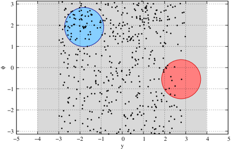
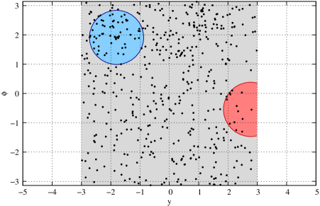
The two other relevant arguments to construct a GhostedAreaSpec object are ghost_area and n_repeat. The ghost_area parameter is the area associated with a single ghost. Smaller values will mean more accurate determinations of the jet area at the cost of a longer CPU-time for clustering. We have found the default ghost area given above to be adequate for most applications, with smaller ghost areas beneficial mainly for high-precision determinations of areas of jets with small $R$.

Since the ghost positions and $p_{t}$’s include small random fluctuations, clustering with different sets of ghosts will give different jet areas. The n_repeat parameter controls how many sets of ghosts will be used. With ${\small\texttt{repeat}}>1$, the final area is averaged over the different sets. For most applications, including those related to pileup mitigation, keeping the default value ${\small\texttt{n\_repeat}}=1$ is a good default. Finally, the other parameters of GhostedAreaSpec control the size of the position and $p_{t}$ fluctuations and can safely be kept to their default values.

Note that, for the sake of reproducibility, facilities are also available to set and retrieve the seeds for the random-number generator. This is done through the set_random_status(...) and get_random_status(...) members of GhostedAreaSpec.

Clustering with areas.

As mentioned above, once an AreaDefinition has been constructed, the clustering with jet-area calculation is obtained using the ClusterSequenceArea class which is constructed using

⬇

template<class L> ClusterSequenceArea(const std::vector<L> & input_particles,

const JetDefinition & jet_def,

const AreaDefinition & area_def);

As long as an instance of this class is in scope, a user can access information about the area of its jets using the following methods of PseudoJet:

⬇

/// Returns the scalar area associated with the given jet

double area = jet.area();

/// Returns the error (uncertainty) associated with the determination of the

/// scalar area of the jet; gives zero when the repeat=1 and for passive/Voronoi areas

double area_error = jet.area_error();

/// Returns the 4-vector area associated with the given jet

PseudoJet area_4vector = jet.area_4vector();

/// When using active_area_explicit_ghosts, returns true for jets made

/// exclusively of ghosts and for ghost constituents.

bool is_pure_ghost = jet.is_pure_ghost();

It is also possible to specify explicitly the set of ghosts to be used provided one directly uses the more basic ClusterSequenceActiveAreaExplicitGhosts class:

⬇

template<class L> ClusterSequenceActiveAreaExplicitGhosts

(const std::vector<L> & pseudojets,

const JetDefinition & jet_def_in,

const std::vector<L> & ghosts,

double ghost_area,

const bool & writeout_combinations = false);

This is useful e.g. to keep area information in tools which require a re-clustering.

2.7.2 Background estimation and subtraction

FastJet natively provide implementations of the two main methods to estimate the background density $\rho$ using equation (2.23).

2.7.2.1 Background estimation.

The simplest workflow for background estimation is first, typically outside the event loop, to create a background estimator. For the grid based method one creates a fastjet::GridMedianBackgroundEstimator,

⬇

#include "fastjet/tools/GridMedianBackgroundEstimator.hh"

// ...

GridMedianBackgroundEstimator bge(double max_rapidity,

double requested_grid_spacing);

where max_rapidity is the maximal $|y|$ covered by the grid and requested_grid_spacing the (requested) grid-cell size.

For the jet-based method, one creates a JetMedianBackgroundEstimator,

⬇

#include "fastjet/tools/JetMedianBackgroundEstimator.hh"

// ...

JetMedianBackgroundEstimator bge(const Selector & selector,

const JetDefinition & jet_def,

const AreaDefinition & area_def);

where the selector is used to indicate which jets are used for background estimation (for most use cases, one just specifies a rapidity range, e.g. SelectorAbsRapMax(4.5) to use all jets with $|y|<4.5$), together with a jet definition and an area definition. An active area with explicit ghosts is recommended.

Both of the above background estimators derive from a fastjet::BackgroundEstimatorBase class and the remaining functionality is common to both. In particular, for each event, one tells the background estimator about the event particles,

⬇

bge.set_particles(event_particles);

where event_particles is a vector of PseudoJet, and then extracts the background density and a measure of its fluctuations with the two following calls

⬇

// the median of ($p_{t}$/area) for grid cells, or for jets that pass the selection cut,

// making use also of information on empty area in the event (in the jets case)

rho = bge.rho();

// an estimate of the fluctuations in the $p_{t}$ density per unit $\smash{\sqrt{A}}$,

sigma = bge.sigma();

2.7.2.2 Background subtraction.

The Subtractor class, defined in include/tools/Subtractor.hh, directly implements the subtraction method (2.24). Its constructor takes a pointer to a background estimator:

⬇

GridMedianBackgroundEstimator bge(....); // or a jet-based estimator

Subtractor subtractor(&bge);

The subtractor can then be used as follows:

⬇

PseudoJet jet;

PseudoJet subtracted_jet = subtractor(jet);

vector<PseudoJet> jets;

vector<PseudoJet> subtracted_jets = subtractor(jets);

The subtractor normally returns jet - bge.rho(jet)*jet.area_4vector(). If jet.pt() is smaller than bge.rho(jet)*jet.area_4vector().pt(), then the subtractor instead returns a jet with zero 4-momentum (so that (subtracted_jet==0) returns true). In both cases, the returned jet retains the user and structural information of the original jet.

Note that the Subtractor has an option

⬇

void set_known_selectors(const Selector & sel_known_vertex,

const Selector & sel_leading_vertex);

The idea here is that there are contexts where it is possible, for some of a jet’s constituents, to identify which vertex they come from. In that case it is possible to provide a user-defined a Selector that indicates whether a particle comes from an identified vertex or not and a second user-defined Selector that indicates whether that vertex was the leading vertex. The 4-momentum from the non-leading vertex is then discarded, that from the leading vertex is kept, and subtraction is applied to component that is not from identified vertices. It follows that $\rho$ must correspond only to the momentum flow from non-identified vertices. With this setup, the jet $p_{t}$ is bounded to be at least equal to that from the leading vertex, as is the mass if the “safe” subtraction option is enabled (see below). The typical application would be CHS events where charged particles would have an identified vertex (see Chapter 11 for more details).

2.7.2.3 Positional dependence of background

The positional dependence can be treated using one of the two techniques introduced in Section 2.4.2 where, now, the properties $\rho$ and $\sigma$ depend on the position of the jet.

In FastJet, the properties of the background are to be obtained through the methods (available for both JetMedianBackgroundEstimator and GridMedianBackgroundEstimator)

⬇

double rho (const PseudoJet & jet); // $p_{t}$ density per unit area $A$ near jet

double sigma(const PseudoJet & jet); // fluctuations in the $p_{t}$ density near jet

Rescaling method.

To account for positional dependence of the background using the “rescaling” technique, one first need to parametrise the average shape of the rapidity dependence from some number of pileup events. Then for subsequent event-by-event background determinations, one carries out a global $\rho$ determination and then applies the previously determined average rescaling function to that global determination to obtain an estimate for $\rho$ in the neighbourhood of a specific jet.

The rescaling approach is available for both grid and jet-based methods. To encode the background shape, the user defines a rescaling function derived from FunctionOfPseudoJet<double> (see the FastJet manual for details). FastJet provides a 4th order polynomial in $y$ as a simple illustrative example:

⬇

// gives rescaling$(y)=1.16+0\cdot y-0.023\cdot y^{2}+0\cdot y^{3}+0.000041\cdot y^{4}$

fastjet::BackgroundRescalingYPolynomial rescaling(1.16, 0, -0.023, 0, 0.000041);

Then one tells the background estimator (whether jet or grid based) about the rescaling with the call

⬇

bge.set_rescaling_class(&rescaling);

Subsequent calls to rho() will return the median of the distribution $p_{t}/A/{\small\texttt{rescaling}}(y)$ (rather than $p_{t}/A$). Any calls to rho(jet) and sigma(jet) will include an additional factor of rescaling$(y_{\small\texttt{jet}})$. Note that any overall factor in the rescaling function cancels out for rho(jet) and sigma(jet), but not for calls to rho() and sigma() (which are in any case less meaningful when a rapidity dependence is being assumed for the background).

Local estimation (jet based).

The “local estimation” technique is available for now only in the case of the jet-based estimator, involves constructing a JetMedianBackgroundEstimator with a Selector retaining only jets in a local range. Such a Selector should be able to take a reference, like SelectorStrip($\Delta y$) which keeps jets in a strip of half-width $\Delta y$ centred on the reference jet. When the user calls either rho(jet) or sigma(jet), jet will be used as the reference for the Selector and only the jets in the event that pass the cut specified by this newly positioned selector are used to estimate $\rho$ or $\sigma$. This method is adequate if the number of jets that pass the selector is much larger than the number of hard jets in the range (otherwise the median $p_{t}/A$ will be noticeably biased by the hard jets). One can attempt to remove some given number of hard jets before carrying out the median estimation, e.g. with a selector such as

⬇

selector = SelectorStrip($\Delta y$) * (!SelectorNHardest(2))

which removes the 2 hardest jets globally and then, of the remainder, takes the ones within the strip. This is however not always very effective, because one may not know how many hard jets to remove.

Estimation in regions (grid based).

The grid-based estimator does not currently provide for local estimates, in the sense that the set of tiles used for a given instance of the grid-based estimator is always fixed. However, as of FastJet 3.1, it is possible to obtain relatively fine control over which fixed set of tiles a grid-based estimator uses. This is done with the help of the RectangularGrid class

⬇

RectangularGrid grid(rap_min, rap_max, rap_spacing, phi_spacing, selector);

GridMedianBackgroundEstimator bge(grid);

A given grid tile will be used only if a massless PseudoJet placed at the centre of the tile passes the selector. So, for example, to obtain an estimate for $\rho$ based on the activity in the two forward regions of a detector, one might set rap_min and rap_min to cover the whole detector and then supply a SelectorAbsRapRange(rap_central_max, rap_max) to select just the two forward regions.

2.7.2.4 Handling masses and safe subtraction

There are several subtleties in handling masses in subtraction. The first is related to the hadrons masses which, as we have seen in Section 2.4.3, requires the introduction of the $\rho_{m}$ property of the background. Since FastJet 3.1, the grid and jet-median background estimators automatically determine $\rho_{m}$ by default. It is returned from a call to rho_m() or rho_m(jet), with fluctuations accessible through sigma_m() or sigma_m(jet). The determination of $\rho_{m}$ involves a small speed penalty and can be disabled with a call to set_compute_rho_m(false) for both background estimators.

To avoid changes in results relative to version 3.0, by default FastJet 3.1 and 3.2 do not use $\rho_{m}$ in the Subtractor, i.e. it uses Eq. (2.24) instead of the more complete Eq. (2.30). However, for a given subtractor, a call to set_use_rho_m(true), will cause it to instead use Eq. (2.30) for all subsequent subtractions. We strongly recommend switching this on if your input particles have masses, and in future versions of FastJet we may change the default so that it is automatically switched on. An alternative is to make the input particles massless.

A second issue, relevant both for Eqs. (2.24) and (2.30), is that sometimes the resulting squared jet mass is negative. This is obviously unphysical. By default the 4-vector returned by the subtractor is left in that unphysical state, so that the user can decide what to do with it. For most applications a sensible behaviour is to adjust the 4-vector so as to maintain its $p_{t}$ and azimuth, while setting the mass to zero. This behaviour can be enabled for a given subtractor by a call to its set_safe_mass(true) function (available since v.3.1). In this case the rapidity is then taken to be that of the original unsubtracted jet.

For situations where “known selectors” have been specified, set_safe_mass(true) will impose stronger constraints: if the transverse momentum of the jet after subtraction is smaller than the transverse momentum from all the known particles from the leading vertex, we set the subtracted 4-momentum to the sum of the known particles coming from the leading vertex. If the subtracted jet has larger transverse momentum but smaller mass, we set the transverse momentum and azimuthal angle of the subtracted jet to the result of the pileup subtraction and set the rapidity and mass from the sum of the known particles coming from the leading vertex. For jets with no known particles coming from the leading vertex, whenever the subtracted 4-vector has an ill-defined rapidity or azimuthal angle, we use those of the original, unsubtracted, jet.

In future versions of FastJet, the default behaviour may be changed so that “safe” subtraction is automatically enabled.

2.7.3 Subtraction for jet shapes

The area–median subtraction procedure for jet shapes introduced in Section 2.5 is not directly included in FastJet but is made available as GenericSubtractor in fjcontrib.

This introduces a class named GenericSubtractor. In practice, the code varies the ghost transverse momentum in order to estimate the derivatives (2.31). Note that to do that, it brings the ghost $p_{t}$ scale from $10^{-100}$ to a value where its effect on the shape is tractable within machine precision.

The basic usage of this class is as follows:

⬇

GenericSubtractor gensub(&some_background_estimator);

FunctionOfPseudoJet<double> shape; // whatever shape you are using

double subtracted_shape_value = gensub(shape, jet);

By default, this only subtracts the transverse momentum density $\rho$ (obtained from the background estimator provided to the class). Two options allow also for the inclusion of the $\rho_{m}$ term: one can either instruct the GenericSubtractor object to compute $\rho_{m}$ from the same background estimator using

⬇

gensub.use_common_bge_for_rho_and_rhom();

or explicitly construct gensub with two background estimators

⬇

GenericSubtractor gensub(& bge_for_rho, & bge_for_rhom);

In all cases, extra information (first order subtraction, derivatives, …) can be retrieved using

⬇

GenericSubtractorInfo info;

double subtracted_shape_value = gensub(shape, jet, info);

(see directly the class definition in GenericSubtractor.hh for details)

Finally, there are some cases where it is possible to use clever tricks to improve the subtraction or its efficiency. The first case is the one when a shape is made of several components and one wishes to subtract each of these components independently rather than subtracting the shape as a whole. (A typical case would be ratios of shapes.) To do that, one derives the shape from ShapeWithComponenents. The second case is the one where the calculation of a shape first partitions the jet into subjets before proceeding to an actual calculation of the shape. To avoid recomputing that partition every time GenericSubtraction varies the ghost scale, one can derive such a shape from the ShapeWithPartition. We refer to the complete documentation of the GenericSubtractor contrib for more details.

2.7.4 Subtraction for fragmentation function moments

The technique to subtract jet fragmentation function moments introduced in Section 2.6 has been implemented in the JetFFMoments contribution to fjcontrib.

It introduces a class, JetFFMoments, which computes the subtracted FF moments for given values of $N$. It is constructed in one of the two following ways:

⬇

/// constructor from a vector of N values, with an optional background estimator

JetFFMoments(const std::vector<double> & ns, JetMedianBackgroundEstimator *bge=0);

/// constructor using nn regularly-spaced values of N between nmin and nmax.

JetFFMoments(double nmin, double nmax, unsigned int nn,

JetMedianBackgroundEstimator *bge=0);

specifying the values of $N$ either explicitly or as a number of values between a minimum and a maximum value. The class can be used to compute just the FF moments, without any form of background subtraction, by not providing a JetMedianBackgroundEstimator to the constructor.

To obtain the FF moments corresponding to a given jet, one uses

⬇

virtual vector<double> operator()(const PseudoJet &jet) const;

virtual vector<double> operator()(const PseudoJet &jet, Info & info) const;

virtual vector<vector<double> > operator()(const vector<PseudoJet> &jets) const;

The first version just returns a vector with the FF moments computed at the requested values of $N$. The third version does the same for a vector of jets. The second version requires an extra argument of the type JetFFMoments::Info which stores potentially useful intermediate information used during the calculation (see the internal contrib’s documentation for details).

We can control how FF moments are normalised using

⬇

void use_scalar_sum(bool use_scalar_sum = true);

void set_return_numerator(bool return_numerator);

void set_denominator(double norm);

The first decides whether the normalisation uses the scalar $p_{t}$ of the jet, $\tilde{p}_{t}$ of the jet $p_{t}$ itself, with the former being the default; the second only computes the numerator (i.e. sets the denominator to 1); and the third sets the denominator to a fixed value, as one would do in, say, $\gamma+$jet events when one wants to use the $p_{t}$ of the photon to normalise the jet FF moments.

Finally, improved subtraction is turned on by calling

⬇

/// kappa is the slope $\kappa$ of $d\sigma/dpt$ parametrised as $\sigma_{0}/\kappa\exp(-p_{t}/\kappa)$

/// in the vicinity of the jet

void set_improved_subtraction(double kappa);

2.8 Recommendations for practical usage

We have introduced all the concepts and ingredients needed to apply the area–median pileup subtraction method. However, at the end of the day, several details have to be specified for a practical use. We give below our recommendations for applications at the LHC and we will provide extensive studies and tests of these settings in the next chapters. For simplicity, we assume that we have events where particles are kept up to a rapidity $|y|=y_{\rm max}$.

Jet area type.

To define the area of the jets, an active area has to be used. We strongly advise the use of explicit ghosts (i.e. an area of the active_area_explicit_ghosts type) which allows for an explicit computation of the contribution from the “empty patches” to (2.23). Furthermore, having ghosts explicitly kept makes possible the calculation of jet areas in more elaborate jet processing like substructure tools. Note that FastJet provides a PseudoJet::is_pure_ghost() method which tells whether a jet is only made of ghosts or not, and a SelectorIsPureGhosts selector which can be used e.g. to eliminate the ghosts when asking for the constituents of a jet.

Ghosts used for jet areas.

Using active areas means that one has to specify the placement of the ghosts. With particles up to $|y|=y_{\rm max}$, we advise to place the ghosts up to a rapidity $y_{\rm max}$ too (see the right of Figure 2.4). We have found that in practice, using a unique set of ghosts, i.e. setting n_repeat=1, is sufficient. It also allows for the set of explicit ghosts to be manipulated in jet tools without ambiguity. For many applications, the default fundamental ghost area, ghost_area, of 0.01 is sufficient. For the production of the final results, it might nevertheless be useful to set this to a smaller value. Although this has a potentially large impact on timings, it also tends to improve the resolution we obtain at the end of the subtraction procedure (see e.g. Fig.4.12). Finally, if one wants to ensure reproducibility, one can always retrieve and set the random seed using GhostedAreaSpec::get_random_status(...) and GhostedAreaSpec::set_random_status(...).

$\mathbf{\rho}$ determination.

We recommend the use of the GridMedianBackgroundEstimator, i.e. the estimation of the background properties based on a grid-based computation of the patches, mainly for speed reasons. We have found that, in practice, a grid size in the range 0.5-0.7 leads to good estimates of $\rho$, with 0.55 (our recommended default) providing a good default across a wide range of processes and pileup conditions.

Positional dependence.

To handle the non-negligible rapidity dependence of pileup (and in the case of heavy-ion collisions, also the azimuthal dependence of the underlying event), we tend to prefer the rescaling method, with local estimation also a useful option e.g. in the case of heavy-ion collisions. Note that, for the sake of convenience, FastJet provides a parametrisation of a 4th order polynomial which has been sufficient for our own studies. This specific form is not meant to be a recommendation and user-defined rescaling functions should be used if the simple function in FastJet fails to describe the positional dependence correctly.

Particle masses.

If you are interested in jet masses and your input particles have non-zero masses, make sure you use the $\rho_{m}$ component in Eq. (2.30) by calling your subtractor’s set_use_rho_m() method. You should also pay attention to what happens with negative squared masses, and consider calling the subtractor’s set_safe_mass() option. For backwards compatibility reasons, both of these options are disabled by default (this may change in versions of FastJet larger than 3.2).

CHS events.

The area–median pileup subtraction technique can also be used in conjunction with Charged-Hadron-Subtracted (CHS) types of events. In that case, all the pileup properties have to be estimated from the neutral particles or from the CHS events directly. Note that, optionally, charged tracks from pileup vertices can be kept as ghosts, i.e. with their momentum scaled down by a large factor. Alternatively, one can cluster the event including the (unmodified) charged tracks from pileup interactions and use something like subtractor.set_known_selectors(SelectorIsCharged(), SelectorIsLeadingVertex()) so that the subtractor itself discards the charged tracks from pileup vertices. CHS events will be discussed at length in Chapter 11.

Subtraction for groomed jets.

For pileup mitigation in jet substructure studies, one usually works with fat jets — i.e. jets of large radius — for which one applies a grooming procedure to clean the soft contamination to the jets. Whenever possible, we strongly recommend to use also the area–median pileup subtractions technique. The main physical reason behind this is that grooming mostly works by reducing the jet area, replacing, say the original $A_{\rm jet}$ into a groomed area $A_{\rm groomed}$. The contamination (2.1) still applies with $A=A_{\rm groomed}$ and the area–median pileup subtraction would correct for it. Many of the common grooming tools have an implementation that supports attaching a Subtractor to them and provide automatic internal pileup subtraction. We will come back to this in our studies in Chapter 7.

Chapter 3 Monte-Carlo validation of approach

In this Chapter, we provide an extensive validation of the area–median pileup subtraction technique based on Monte-Carlo studies. Our goal is to validate two key aspects of the area–median method: (i) that it indeed corrects for pileup contamination and does it for a wide range of jet observables, (ii) that it is a robust method, fairly insensitive to variations of the pileup conditions and details of the hard event over wide kinematic ranges. We also want to justify our recommendations outlined in Section 2.8.

Before entering into this vast territory, we shall first briefly discuss the basic pileup properties $\rho$ and $\sigma$. This is meant to build a cleaner quantitative picture of pileup effects and is done in Section 3.1. We shall then perform Monte Carlo studies of the area–median performance for several observables and several environments.

• The jet $p_{t}$ (Section 3.2). This is by far the most common application, relevant for the vast majority of LHC analyses.

• Jet shapes (Section 3.3). This includes the jet mass as well as a series of other (infrared-and-collinear safe) jet observables, used in more specific LHC analyses.

• Heavy-ion Underlying Events (Chapter 4). We will show that the area–median method is also suited to subtract the overwhelming Underlying Event created in heavy-ion collisions at RHIC and at the LHC. This also includes a series of interesting analytic estimates in Section 4.4 which could also be relevant for applications to pileup subtraction in proton-proton collisions.

• Jet fragmentation function (Section 4.7). Still using heavy-ion collisions, we validate our subtraction method for fragmentation function moments.

For all these studies, we will explore various kinematic dependencies so as to assess the robustness of the area–median subtraction method. This includes varying the pileup multiplicity, the jet transverse momentum and rapidity, but also checking that the jet multiplicity in the hard event does not introduce large biases. On top of that, we also want to make sure that our findings do not depend on the specific details of Monte-Carlo generators. In the end, this translates into rather CPU-expensive simulations. Even though some of the simulations performed in the context of the original publications are slightly out of date (e.g. use old versions of Monte Carlo generators and tunes, or use different collision energies), we have decided to keep the original results and not update them to a more modern setup except for our study of the jet transverse momentum. There are several reasons justifying this approach. First, as already mentioned, the jet transverse momentum is by far the most important use-case and so we consider that it is important to revisit the original study done in [7] with a more modern setup. This is also the study that provides most of the bases for our recommendations in Section 2.8, again justifying an up-to-date series of Monte-Carlo studies. Once this important baseline has been established, we will have a clear indication that the area–median subtraction procedure is robust and insensitive to the details of the simulation. We have therefore estimated that it was not critical to update the other Monte Carlo studies. We will discuss more at the beginning of each section the differences between the original simulations, the current (experimental) situation and the results presented in this document.

3.1 Properties of the pileup density

Figure 3.1: Rapidity dependence of the background density $\rho$ calculated on minimum bias events as obtained by Pythia 8 with the tune 4C. Left: $\rho$ profile; right: $\rho_{m}$ profile. For all plots, we show the results for the 3 LHC energies, $\sqrt{s}=7,8$ and $13$ TeV. The dashed lines on the rightmost plots represent the result of fitting $\rho$ with a fourth order polynomial as in Eq. (3.1) and rescaling it so that it matches at $y=0$.

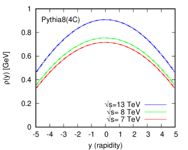
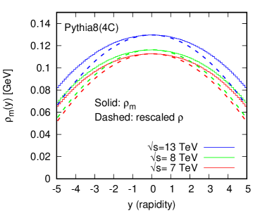
Before digging into the systematic validation of the area–median pileup subtraction technique, it is useful to have a quantitative idea of how large we should expect the pileup contamination to be.

In the case of pileup in $pp$ collisions, we can estimate directly the pileup contamination from minimum bias collisions.

The first result of such a study is presented in Fig. 3.1. We have used Pythia 8.186 [55], with tune 4C [56], to generate minimum bias events for the three main LHC centre-of-mass energies: 7, 8, and 13 TeV. Let us first look at the leftmost plot, which shows the average transverse momentum density $\rho$ in the event as a function of rapidity. In this case, it has been computed exactly, in each rapidity bin of width 0.1, from the minimum bias events. We see that, in central rapidity, each pileup event would, on average bring around 700 MeV at 7-8 TeV and around 900 MeV at 13 TeV. This drops down by about a factor of 2 if we go to forward rapidities, $|y|=5$. The next average property of pileup that we have discussed is $\rho_{m}$, the contribution from particle masses, or, more precisely, from $m_{t}-p_{t}$. This is shown on the right plot of Fig. 3.1 and it indicates that it is only about 15% of the transverse component $\rho$.

$\sqrt{s}$	$a$	$b$	$c$
7 TeV	0.7161921	-0.0159483	1.01133$\times 10^{-5}$
8 TeV	0.7538506	-0.0164948	1.44286$\times 10^{-5}$
13 TeV	0.9084412	-0.0189777	4.05981$\times 10^{-5}$

Table 3.1: Coefficients of the fit of the rapidity profile $\rho(y)$, Eq. (3.1) for the three centre-of-mass energies under consideration.

To handle the rapidity dependence of pileup when using the area–median subtraction method, we have seen that one approach is to use a rescaling function. The rescaling function itself can be readily extracted from minimum bias data. The profiles we obtain on Fig. 3.1 can very well be approximated by a fourth degree polynomial of the form

$$\rho(y)=(a+by^{2}+cy^{4})\>\text{GeV}.$$ (3.1)

The fitted parameters for the different centre-of-mass energies are given in Table 3.1.

On the rightmost plot of Fig. 3.1, we have shown, using dashed lines, the result of rescaling the $\rho$ rapidity profile so that it matches $\rho_{m}$ at $y=0$. We see that it reproduces the $\rho_{m}$ rapidity dependence within about 15%.

Figure 3.2: Rapidity dependence of the background fluctuations between different events ($\sigma_{\rho}$, left plot) and inside an event ($\sigma$, right plot).

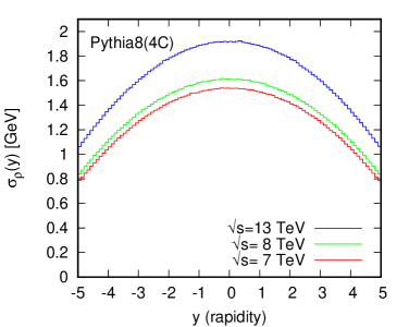
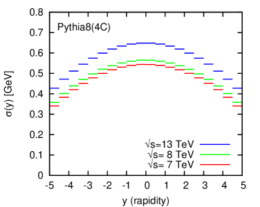
Let us now move to the other fundamental properties of pileup, namely measures of its fluctuations: $\sigma_{\rho}$ (between events) and $\sigma$ (inside an event). The former is the simplest to measure: we just look at the dispersion of $\rho(y)$ across our event sample. The result is plotted on the left panel of Fig. 3.2 and it shows large fluctuations, reaching about 1.5 GeV for Run I energies and nearly 2 GeV at 13 TeV. Next, to estimate $\sigma$ in a given rapidity range $y_{1}<y<y_{2}$, we split the azimuthal angle range in several (25) cells and compute the dispersion of the cell scalar $p_{t}$ divided by the square root of the cell area is an estimate of $\sigma$. The resulting rapidity distribution for $\sigma$ is plotted on the right panel of Fig. 3.2. It shows a similar shape than $\rho$, and reaches $\sim$500 (resp. $\sim$650) MeV at central rapidities for 7 TeV (resp. 13 TeV) collisions.

Figure 3.3: Distribution of the true pileup density $\rho$ computed for $|y|<0.5$ with Poisson-distributed events with $\mu=\langle{N_{\mathrm{PU}}}\rangle=25$. The dotted line represents a Gaussian fit with the average and dispersion indicated on the plot.

Figure 3.4: Evolution of the pileup fundamental properties as a function of $N_{\mathrm{PU}}$. The properties are averaged for $|y|<2.5$.

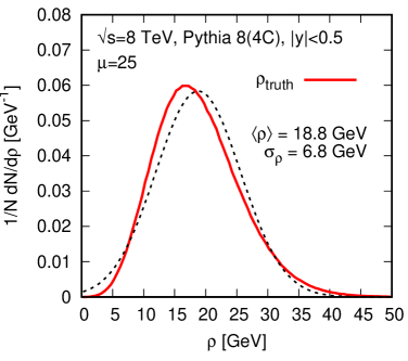
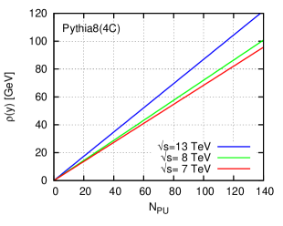
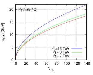
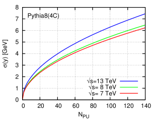
One might also wonder how precisely the distribution of the pileup density $\rho$ in a given event is characterised by its average density $\langle\rho\rangle$ and its fluctuations $\sigma_{\rho}$. This is illustrated in Fig. 3.3 where we looked at the $\rho$ distribution for a sample of Poisson-distributed pileup events. The dotted line, corresponding to a Gaussian fit, shows a reasonable description of the Monte-Carlo results. The Gaussian approximation appears therefore good enough for the simple analytic estimates we do in this document.

It is a trivial exercise to infer from the above numbers the pileup dependence of $\rho$, $\sigma_{\rho}$ and $\sigma$. Based on our introductory discussion, we know that $\rho$ will scale like $N_{\mathrm{PU}}$ while $\sigma_{\rho}$ and $\sigma$ scale like $\sqrt{{N_{\mathrm{PU}}}}$. To illustrate this, we have averaged the minimum bias properties in the central region, between $|y|=0$ and $|y|=2.5$. The expected $N_{\mathrm{PU}}$ scaling is plotted on Fig. 3.4 for $\rho$, $\sigma_{\rho}$ and $\sigma$ respectively. If, for the sake of the argument, we assume that a jet of radius $R$ has an area $\pi R^{2}$, which is a good approximation for the standard anti-$k_{t}$ jets, the pileup contamination into a jet can be inferred from these curves by multiplying $\rho$ and $\sigma_{\rho}$ by $A=\pi R^{2}$ and $\sigma$ by $\sqrt{A}=\sqrt{\pi}R$. For a typical jet obtained with $R=0.4$, this gives $A\approx 0.5$ and $\sqrt{A}\approx 0.7$.

3.2 Widest application: the jet transverse momentum

By far the most widely used property of a jet for which pileup subtraction is mandatory is its transverse momentum. It is used in a majority of analyses at the LHC. We shall therefore begin our systematic study of the area–median method by a study of its performance for the jet $p_{t}$.

This study serves different purposes. First, it is meant to be a validation of the area–median approach. To that aim, we shall also consider an alternative approach, based on the number of observed pileup vertices. Next, we want to study the various approaches presented in the previous Chapter to handle the positional dependence of $\rho$. Finally, we want to assess the robustness of the method so we shall use a wide range of hard processes — this is crucial since it is supposed to be used across the whole range of analyses at the LHC — and test different Monte-Carlo generators in order to estimate the uncertainty on our conclusions.

Most of the study presented below comes from a contribution to the proceedings of the 2011 Physics at TeV colliders workshop in Les Houches. However, since the reconstruction of the jet transverse momentum is used in such a wide variety of LHC analysis, we have renewed our studies with more realistic conditions for the run I of the LHC. Compared to the original study, we have moved from 7 to 8 TeV for the centre-of-mass collision energy, extended our range of $N_{\mathrm{PU}}$ to 50 (instead of 30) and used $\mu=25$ as an average pileup multiplicity instead of 10. Note that, while conducted at 8 TeV, the features observed below are not expected to be significantly altered at 13 TeV. We will see some example studies carried at 13 TeV in the last part of this document where we shall discuss more elaborate techniques for Run II and beyond.

3.2.1 Subtraction techniques

Since we want to validate the various aspects of the area–median method, we shall test both the jet-based and the grid-based approaches, as well as several approaches to handling the positional dependence. In order to provide a baseline for comparison and discussion, we shall also test a simpler alternative based on the number of (seen) pileup vertices.

In all cases, the subtraction of the jet transverse momentum will be done through the central formula, Eq. (2.24), and define the subtracted jet transverse momentum using

$$p_{t,\rm sub}=p_{t}-\rho_{\rm est}A$$ (3.2)

where $\rho_{\rm est}$ is the estimated value for the background density per unit area. The various methods we put under scrutiny here only depend in how they estimate $\rho_{\rm est}$.

Using seen vertices.

Since experimentally it might be possible — within some level of accuracy that goes beyond the scope of this discussion — to count the number of pileup vertices using charged tracks, one appealing way to estimate the background density in a given event would be to count these vertices and subtract a pre-determined number for each of them:

$$\rho_{\rm est}^{({N_{\mathrm{PU}}})}(y)=f(y)\,N_{\rm PU,seen},$$ (3.3)

where we have made explicit the fact that the proportionality constant $f(y)$ can carry a rapidity dependence. $f(y)$ can be studied from minimum bias collisions (see the previous Section) and can take into account the fact that not all the PU vertices will be reconstructed.

Area–median subtraction.

This estimates the background using the central formula (2.23):

$$\rho_{\rm est}^{\rm(global)}=\underset{i\in\,\rm patches}{\rm median}\left\{\frac{p_{t,i}}{A_{i}}\right\}$$ (3.4)

We shall test both jets and grid cells as patches.

Area–median with a local range.

This uses a local estimate of the area–median background-density as obtained from Eq. (2.25). A typical example, that we shall study later on, is the case of a strip range where only the jets with $|y-y_{j}|<\Delta$ are included.

Area–median with rescaling.

This is the other option to correct for the positional dependence. It uses Eq. (2.27). The rescaling $f(y)$ can be taken directly from Section 3.1.

3.2.2 Testing framework

Embedding.

The remainder of this Section is devoted to an in-depth comparison of the subtraction methods proposed above. Our testing framework goes as follows. First, we embed a hard event into a pileup background, either with a fixed number $N_{\mathrm{PU}}$ of minimum-bias events or with a Poisson-distributed number of pileup interactions, with $\mu$ pileup events on average. Then, we reconstruct and subtract the jets in both the hard and full events. Jets in the hard (resp. full) event will be referred to as hard jets (resp. full jets) and the kinematic cuts are applied on the hard jets.

Matching.

Testing Eq. (3.5) requires that we match the jets in the full event (optionally subtracted) with the jets in the initial hard event. For each of the full jets, we do that by finding a hard jet such that their common constituents contribute for at least 50% of the transverse momentum of the hard jet. Compared to a matching where we use distances between the jet axes, this has the advantage that a given hard jet is matched to at most one jet in the full event, and it avoids the arbitrariness of choosing a threshold for the matching distance. Also, this matching is independent of the subtraction procedure.

Quality measures.

For a matched pair of jets, we shall use the notation $p_{t}^{\rm hard}$ and $p_{t}^{\rm full}$ for the transverse momentum of the jet in the hard and full event respectively, and $p_{t}^{\rm hard,sub}$ and $p_{t}^{\rm full,sub}$ for their subtracted equivalents. We can then compute the shift

$$\Delta p_{t}=p_{t}^{\rm full,sub}-p_{t}^{\rm hard,sub},$$ (3.5)

i.e. the difference between the reconstructed-and-subtracted jet with and without pileup. A positive (resp. negative) $\Delta p_{t}$ would mean that the PU contamination has been underestimated (resp. overestimated). Though in principle there is some genuine information in the complete $\Delta p_{t}$ distribution — e.g. it could be useful to deconvolute the extra smearing brought by the pileup, see e.g. [6] and [58] and the discussion in Chapter 4 below — we shall mainly focus on two simpler quantities: the average shift $\langle\Delta p_{t}\rangle$ and the dispersion $\sigma_{\Delta p_{t}}$. While the first one is a direct measure of how well one succeeds at subtracting the pileup contamination on average, the second quantifies the remaining effects on the resolution. One thus wishes to have $\langle\Delta p_{t}\rangle$ close to 0 and $\sigma_{\Delta p_{t}}$ as small as possible. Note that these two quantities can be studies as a function of variables like the rapidity and transverse momentum of the jets or the number of pileup interactions. In all cases, a flat behaviour would indicate a robust subtraction method.

Instead of these quality measures, some studies in the literature (see e.g. [11]), prefer to use the correlation coefficient between $p_{t}^{\rm full,sub}$ and $p_{t}^{\rm hard,sub}$. We find that quantitative interpretations of correlation coefficients can sometimes be delicate, essentially because they combine the covariance of two observables with the two observables’ individual variances. this is further discussed in Appendix C). To the exception of Chapter 11, we will thus use $\langle\Delta p_{t}\rangle$ and $\sigma_{\Delta p_{t}}$ as indicators of the performance of pileup mitigation techniques.

Robustness.

The robustness of our conclusions can be checked by varying many parameters:

• one can study various hard processes to check that the PU subtraction is not biased by the hard event. In what follows we shall study dijets with $p_{t}$ ranging from 20 GeV to 1 TeV, as well as fully hadronic $t\bar{t}$ events as a representative of busier final states.

• The Monte-Carlo used to generate the hard event and PU can be varied. For the hard event, we have used Pythia 6.4.28 with the Perugia 2011 tune [59], Pythia 8.186 [55] with tune 4C [56] and Herwig 6.5.10 [60, 61] with the ATLAS tune and we have switched multiple interactions on (our default) or off. For the minimum bias sample used to generate PU, we have used Pythia 8, tune 4C.

Additional details of the analysis.

For the sake of completeness, we list here the many other details of how the $\Delta p_{t}$ analysis has been conducted. We have considered particles with $|y|\leq 5$ with no $p_{t}$ cut or detector effect; jets have been reconstructed with the anti-$k_{t}$ algorithm with $R=0.5$ keeping jets with $|y|\leq 4$; for area computations, we have use active areas with explicit ghosts with ghosts placed up to $|y|=5$. For jet-based background estimations, we have used the $k_{t}$ algorithm with $R=0.4$ though other options will be discussed (and the 2 hardest jets in the set have been excluded from the median computation to reduce the bias from the hard event); for grid-based estimations the grid extends up to $|y|=5$ with cells of edge-size 0.55 (other sizes will be investigated). For estimations using a local range, a strip range of half-width 1.5 has been used (again excluding the two hardest jets in the strip) and for estimations using rapidity rescaling, we have used the results obtained in the previous Section (see e.g. Table. 3.1). Jet reconstruction, area computation and background estimation have all been carried out using FastJet (v3.1) [17, 18]. Whenever we quote an average pileup multiplicity, pileup is generated as a superposition of a Poisson-distributed number of minimum bias events and we will vary the average number of pileup interactions. We shall always assume $pp$ collisions with $\sqrt{s}=8$ TeV.

For the “seen vertices” pileup subtraction, we need to provide a proper definition of what we call “seen vertices”. In what follows, we shall define that as a minimum bias interaction that has at least 2 charged tracks with $|y|\leq 2.5$ and $p_{t}\geq 100$ MeV, which corresponds to 69.7% of the events.

3.2.3 Generic performance and rapidity dependence

Figure 3.5: fraction of the jets in the hard event, passing the $p_{t}$ cut, which have been matched to a jet in the full event. Different curves correspond to different processes. Efficiencies are shown as a function of the number of pileup interactions.

       

Figure 3.6: Left: distribution of difference between the estimated $\rho$, $\rho_{\rm est}$, and its true value in the $|y|<0.5$ rapidity interval. The calculation is done using an average of 25 Poisson-distributed pileup events for a dijet sample generated with a generator $p_{t}$ cut of 40 GeV. The dashed (black) line corresponds to the area–median estimation (using a rapidity-rescaled grid estimator) while the solid (magenta) line corresponds to the “seen vertices” estimate. The numbers indicated inside brackets in the legend correspond to the average and dispersion of the corresponding distributions. Right: the corresponding $\Delta p_{t}$ distribution for anti-$k_{t}$($R=0.5$) jets above 50 GeV. We have also added the distribution obtained when no subtraction is performed (solid, green, line).

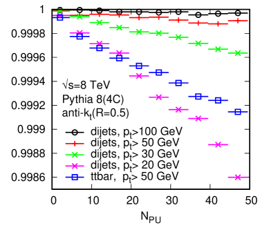
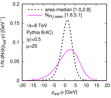
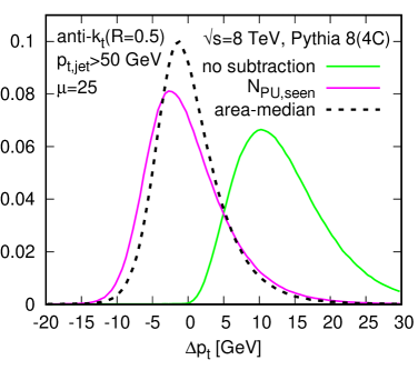
The first thing we want to look at is the matching efficiency between the hard and full jets. This is shown in Fig. 3.5 where we plot, as a function of $N_{\mathrm{PU}}$ and for different processes, the fraction of hard jets which have been matched to a jet in the full event. We see that even with busy events and high pileup multiplicities, the matching efficiencies remain very high, always above 99.85% and often much higher. As for the $p_{t}$ dependence, the matching efficiency quickly goes close to 1 when $p_{t}$ increase, with again large matching efficiencies all the way down to jets of 20 GeV.

Before we focus on the quality measured, $\langle\Delta p_{t}\rangle$ and $\sigma_{\Delta p_{t}}$, averaged over event samples, let us first have a brief look at global distributions. A few illustrative examples are presented in Fig. 3.6. On the left plot, we directly plot the quality of the background estimation at central rapidity. We see that both the area–median estimate and the “seen vertices” estimate are close to the actual, true, $\rho$. The width of these distributions show that the area–median tends to give a better estimate than the “seen vertices” approach. On the right plot, we show how this translates in a more practical situation where we subtract pileup contamination from a sample of jets above 50 GeV. In this case, we have also included the unsubtracted distribution which is clearly biased and wider than both subtracted ones. Overall, all these distributions can be well-approximated by Gaussian distributions and we can safely use the averaged quantities $\langle\Delta p_{t}\rangle$ and $\sigma_{\Delta p_{t}}$ to assess the performance and robustness of the various subtractions methods.

Let us therefore carry on with more detailed performance benchmarks, starting with the study of the rapidity dependence of PU subtraction. Fig. 3.7 shows the residual average shift ($\langle\Delta p_{t}\rangle$) as a function of the rapidity of the hard jet. These results are presented for different hard processes, generated with Pythia 8 (v8.186) and using Poisson-distributed pileup with $\mu=25$. Robustness w.r.t. that choice will be discussed in the next Section but does not play any significant role for the moment.

Figure 3.7: Residual average shift as a function of the jet rapidity for all the considered subtraction methods. For the left (resp. centre, right) plot, the hard event sample consists of dijets with $p_{t}\geq 50$ GeV (resp. dijets with $p_{t}\geq 400$ GeV, and jets above $p_{t}\geq 50$ GeV in $t\bar{t}$ events), generated with Pythia 8 (tune 4C) in all cases. The typical PU contamination (for unsubtracted jets) is around 14 GeV at central rapidities.

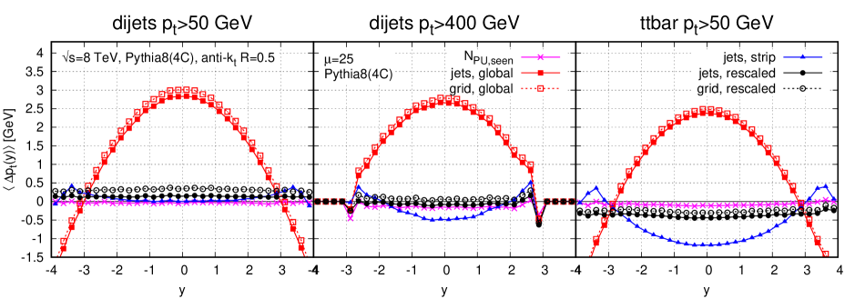
The first observation is that the subtraction based on the number of seen PU vertices does a very good job in all 3 cases. Then, global area–median (using jets or grid cells) estimations of $\rho$, i.e. the (red) square symbols, do a fair job on average but, as expected, fail to correct for the rapidity dependence of the PU contamination. If one now restricts the median to a rapidity strip around the jet, the (blue) triangles, or if one uses rapidity rescaling, the (black) circles, the residual shift is very close to 0, typically a few hundreds of MeV, and flat in rapidity.

Note that the strip-range approach seems to have a small residual rapidity dependence and overall offset for high-$p_{t}$ processes or multi-jet situations. That last point may be due to the fact that smaller ranges tend to be more affected by the presence of the hard jets (see also Section 5.2), an effect which is reinforced for multi-jet events. The fact that the residual shift seems a bit smaller for grid-based estimates will be discussed more extensively in the next Section.

Next, we turn to the dispersion of $\Delta p_{t}$, a direct measure of the impact of PU fluctuations on the $p_{t}$ resolution of the jets. Our results are plotted in Fig. 3.8 as a function of the rapidity of the hard jet (left panel), the number of PU vertices (central panel) and the transverse momentum of the hard jet (right panel). All subtraction methods have been included as well as the dispersion one would observe if no subtraction were performed.

The results show a clear trend: first, a subtraction based on the number of seen PU vertices brings an improvement compared to not doing any subtraction; second, area–median estimations of $\rho$ give a more significant improvement; and third, all area–median approaches perform similarly well (with a little penalty for global approaches).

The reason why the area–median estimations of $\rho$ outperform the estimation based on the number of seen PU vertices is simply because minimum bias events do not all yield the same energy deposit and this leads to an additional source of fluctuations in the “seen vertices” estimation compared to all area–median ones. This is the main motivation for using an event-by-event determination of $\rho$ based on the energy deposited in the event. This motivation is further strengthened by the fact that additional issues like vertex resolution or out-of-time PU would affect both $\langle\Delta p_{t}\rangle$ and $\sigma_{\Delta p_{t}}$ if estimated simply from the number of seen vertices while area–median approaches are more robust.

Figure 3.8: Dispersion $\sigma_{\Delta p_{t}}$. Each curve corresponds to a different subtraction method and the results are presented as a function of different kinematic variables: left, as a function of the rapidity of the hard jet for a sample of jets with $p_{t}\geq 100$ GeV and assuming an average of 25 PU (Poisson-distributed) events; centre: as a function of the number of PU events for a sample of jets with $p_{t}\geq 100$; right: as a function of the $p_{t}$ of the hard jet, assuming again an average of 25 PU events

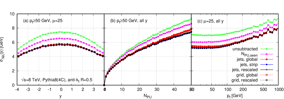
Note that even though local ranges and rapidity rescaling do correct for the rapidity dependence of the PU on average, the dispersion still depends on rapidity. The increase with the number of PU vertices is in agreement with the expected $\sqrt{{N_{\mathrm{PU}}}}$ behaviour and the increase with the $p_{t}$ of the hard process can be associated with back-reaction, see the next Section as well as Section 4.4.1. These number can also be compared to the typical detector resolutions which would be $\sim$10 GeV for 100 GeV jets and $\sim$20 GeV at $p_{t}=400$ GeV [63, 64].

3.2.4 Digression: back-reaction effects

Figure 3.9: Contribution of the back-reaction to the pileup average shift and dispersion.

Figure 3.10: Dispersion $\sigma_{\Delta p_{t}}$ broken into two contributions: the back-reaction contribution and the remaining contribution due intrinsically to residual pileup fluctuations. The left plot shown dijet events as a function of the jet $p_{t}$, the right plot focuses on $t\bar{t}$ events as a function of the number of pileup interactions.

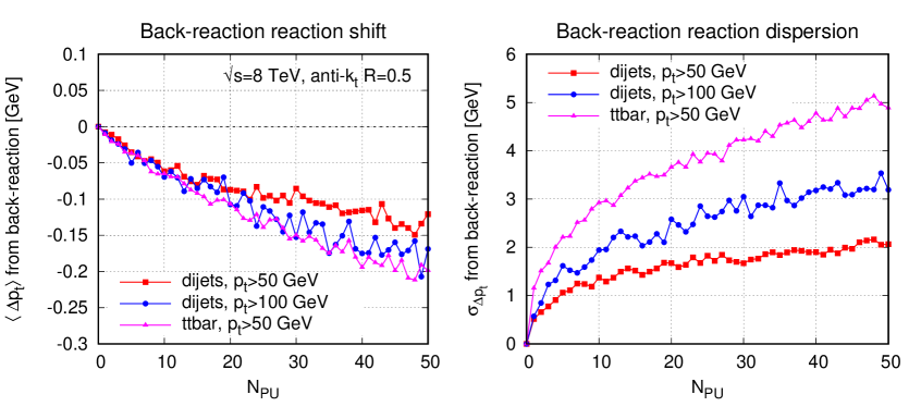
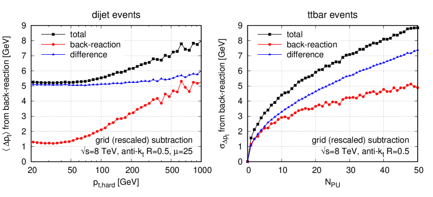
Remember that back-reaction is the effect of pileup on the clustering of the particles from the hard interaction themselves. This effect is independent of the subtraction method. In this short Section, we discuss a few of the quantitative effects of back-reaction on the jet transverse momentum and compare them to the average shift and dispersion quoted in the previous Section.

The determination of the back reaction works as follows: for each pair of matching hard and full jets, we look at the particles from the full jet that come from the hard interaction, say $p_{t}^{\text{hard-in-full}}$. The back-reaction is then computed for each jet as

$$\Delta p_{t}^{\text{back-reaction}}=p_{t}^{\text{hard-in-full}}-p_{t}^{\rm hard}.$$ (3.6)

We can then, as before, look at the average shift and dispersion due to back-reaction. These are shown in Figure 3.9. We see that, as expected, the effect of back-reaction on the average shift is very small (less than 200 MeV). We also see that it comes with a non-negligible dispersion effect, in particular for busy events ($t\bar{t}$) or high-$p_{t}$ jets.

To investigate this a little further, it is interesting to look at the contribution of back-reaction to the overall dispersion observed in Fig. 3.8. This is shown in Fig. 3.10 for dijet events as a function of the jet $p_{t}$ and for $t\bar{t}$ events as a function of the number of pileup interactions. In both cases, the total dispersion (the black curve) is as obtained with the rescaled grid subtraction in Fig. 3.8. The back reaction is as shown in Fig. 3.9. The difference, computed as $[\sigma_{\Delta p_{t}}^{2}-(\sigma_{\Delta p_{t}}^{\mathrm{BR}})^{2}]^{\frac{1}{2}}$, can be directly associated with background fluctuations and misestimation of $\rho$. One sees that the background-fluctuation component dominates over the back-reaction component although the latter is certainly non-negligible. In particular, it is the back-reaction component which is mainly responsible for the rise of the dispersion with the jet $p_{t}$, with a mostly-$p_{t}$-independent background-fluctuation contribution.

This is the case because the back-reaction dispersion is dominated by rare events in which two similarly hard subjets are separated by a distance close to $R$ (specifically by $R\pm\epsilon$ with $\epsilon\ll 1$). In such a configuration, the background’s contribution to the two subjets can affect whether they recombine and so lead to a large, ${\cal O}\left(p_{t}\right)$, change to the jet’s momentum. In the limit of a uniform background, $\sigma/\rho\ll 1$, this can be shown (see Section 5.1.3 for details) to occur with a probability of order $\alpha_{s}\rho R^{2}/p_{t}$. Thus the contribution to the average shift $\left\langle\Delta p_{t}\right\rangle$ is proportional to $\alpha_{s}\rho R^{2}$, while the contribution to $\left\langle\Delta p_{t}^{2}\right\rangle$ goes as $\alpha_{s}\rho R^{2}p_{t}$, and so leads to a dispersion that should grow asymptotically as $\sqrt{p_{t}}$ (fig. 3.10 is, however, probably not yet in the asymptotic regime).

It is worth keeping in mind that even though rare but large back-reaction dominates the overall dispersion, it will probably not be the main contributor in distorting the reconstructed jet spectrum. Such distortions come from upwards $\Delta p_{t}$ fluctuations, whereas large back-reaction tends to be dominated by downwards fluctuations. The reason is simple: in order to have an upwards fluctuation from back-reaction, there must be extra $p_{t}$ near the jet in the original $pp$ event. This implies the presence of a harder underlying $2\to 2$ scattering than would be deduced from the jet $p_{t}$, with a corresponding significant price to pay in terms of more suppressed matrix elements and PDFs. We shall show a similar behaviour for heavy-ion collisions and discuss analytic results in more details in Section 5.1.3.

3.2.5 Robustness and Monte-Carlo dependence

Figure 3.11: Dependence of the average $p_{t}$ shift as a function of the number of PU vertices for various Monte-Carlo generators. For the left plot, the hard sample is made of dijets with $p_{t}\geq 100$ GeV while for the right plot, we have used a hadronic $t\bar{t}$ sample. For each generator, we have considered both the case with the Underlying Event switched on (filled symbols) and off (open symbols). All results have been obtained using a grid-based median estimation of $\rho$ using rapidity rescaling.

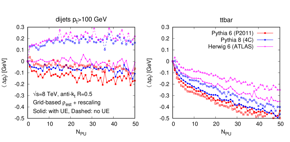
The last series of results we want to present addresses the stability and robustness of the area–median estimation of the PU density per unit area.

To do that, the first thing we shall discuss is the Monte-Carlo dependence of our results. In Fig. 3.11 we compare the different Monte-Carlo predictions for the $\langle\Delta p_{t}\rangle$ dependence on the number of PU vertices in the case of a grid-based median estimate of $\rho$ with rapidity rescaling. For each of the three considered Monte-Carlos, we have repeated the analysis with and without Underlying Event (UE) in the hard event. The first observation is that all the results span a range of 300-400 MeV in $\Delta p_{t}$ and have a similar dependence on the number of PU vertices. The dependence on ${N_{\mathrm{PU}}}$ is flat for dijet events but shows a small decrease for busier events. The 300-400 MeV shift splits into a 100-200 MeV effect when changing the generator, which is likely due to the small but non-zero effect of the hard event on the median computation, and a 100-200 MeV effect coming from the switching on/off of the UE.

Figure 3.12: Average shift, $\langle\Delta p_{t}\rangle$, plotted as a function of the jet $p_{t}$ for an average of 25 PU events (left), or as a function of the number of PU vertices for dijets with $p_{t}\geq 100$ GeV (centre) and for $t\bar{t}$ events (right). In all cases, we compare 3 methods: the rapidity-strip range, (red) triangles, the jet-based approach with $y$ rescaling, (blue) circles, and the grid-based approach with $y$ rescaling, (black) squares. Each curve is the result of averaging over the various Monte-Carlo generator options. Their dispersion is represented both as error bars on the top row and directly on the bottom row.

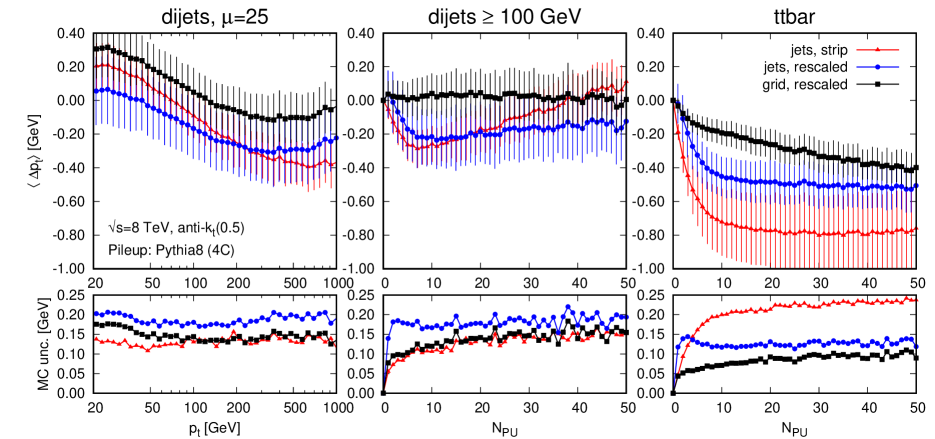
This question of subtracting the UE deserves a discussion: since the UE is also a soft background which is relatively uniform, it contributes to the median estimate and, therefore, one expects the UE, or at least a part of it, to be subtracted together with the PU. Precisely for that reason, when we compute $\Delta p_{t}$, our subtraction procedure is not applied only on the “full jet” (hard jet+PU) but also on the hard jet, see Eq.(3.5). The 100-200 MeV negative shift observed in Fig. 3.11 thus means that, when switching on the UE, one subtracts a bit more of the UE in the full event (with PU) than in the hard event alone (without PU). This could be due to the fact (see Section 5.2 for details) that for sparse events, as is typically the case with UE but no PU, the median tends to slightly underestimate the “real” $\rho$, e.g. if half of the event is empty, the median estimate would be 0. This is in agreement with the fact that for $t\bar{t}$ events, where the hard event is busier, switching on the UE tends to have a smaller effect. Note finally that as far as the size of the effect is concerned, this 100-200 MeV shift has to be compared with the $\sim$1 GeV contamination of the UE in the hard jets.

Finally, we wish to compare the robustness of our various subtraction methods for various processes i.e. hard events and PU conditions. In order to avoid multiplying the number of plots, we shall treat the Monte-Carlo (including the switching on/off of the UE) as an error estimate. That is, an average measure and an uncertainty will be extracted by taking the average and dispersion of the 6 Monte-Carlo setups. The results of this combination are presented on Fig. 3.12 for various situations and subtraction methods. For example, the 6 curves from the left plot of Fig. 3.11 have been combined into the (black) squares of the central panel in Fig. 3.12.

Two pieces of information can be extracted from these results. First of all, for dijets, the average bias of PU subtraction remains very small and, to a large extent, flat as a function of the $p_{t}$ of the jets and the number of PU vertices. When moving to multi-jet situations, we observe an additional residual shift in the 100-300 MeV range, extending to $\sim$500 MeV for the rapidity-strip-range method. This slightly increased sensitivity of the rapidity-strip-range method also depends on the Monte-Carlo. While in all other cases, our estimates vary by $\sim$ 100 MeV when changing the details of the generator, for multi-jet events and the rapidity-strip-range approach this is increased to $\sim$200 MeV.

Overall, the quality of the subtraction is globally very good. Methods involving rapidity rescaling tends to perform a bit better than the estimate using a rapidity strip range, mainly a consequence of the latter’s greater sensitivity to multi-jet events. In comparing grid-based to jet-based estimations of $\rho$, one sees that the former gives slightly better results, though the differences remain small.

Since the grid-based approach is considerably faster than the jet-based one, as it does not require an additional clustering of the event, the estimation of $\rho$ using a grid-based median with rapidity rescaling comes out as a very good default for PU subtraction. One should however keep in mind local-range approaches for the case where the rapidity rescaling function cannot easily be obtained.

3.2.6 PU v. UE subtraction: an analysis on $Z$+jet events

To give further insight on the question of what fraction of the Underlying Event gets subtracted together with the pileup, we have performed an additional study of $Z+$jet events. We look at events where the $Z$ boson decays into a pair of muons. We have considered 5 different situations: events without PU or UE, events with UE but no PU with and without subtraction, and events with both UE and PU again with and without subtraction. Except for the study of events without UE, this analysis could also be carried out directly on data.

Figure 3.13: Left: relative difference between the reconstructed jet and the reconstructed $Z$ boson transverse momenta. Right: at a given $p_{t}$ of the reconstructed $Z$ boson, difference between the reconstructed $p_{t}$ of the jet and the ideal $p_{t}$ with no UE or PU, i.e. $p_{t}$ shift w.r.t. the “noUE” curve, the (black) triangles, on the left panel. See the text for the details of the analysis.

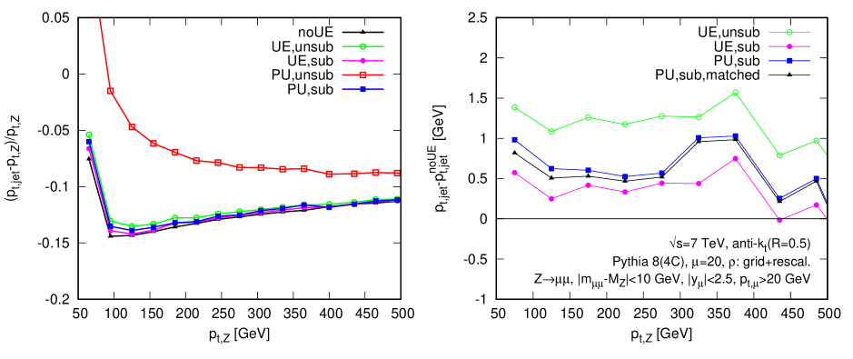
Practically, we impose that both muons have a transverse momentum of at least 20 GeV and have $|y|\leq 2.5$, and we require that their reconstructed invariant mass is within 10 GeV of the nominal $Z$ mass. As previously, jets are reconstructed using the anti-$k_{t}$ jet algorithm with $R=0.5$ and the pileup subtraction is performed using the grid-based-median approach with rapidity rescaling and a grid size of 0.55. All events have been generated at $\sqrt{s}=7$ TeV with Pythia 8 (tune 4C) and we have assumed an average PU multiplicity of 20 events. Note that for this study, no matching between the hard and full events are required. In practice, we only focus on the hardest jet in the event, with the cut applied after the area–median subtraction for the subtracted cases.

In Fig. 3.13, we have plotted the ratio $p_{t,\rm jet}/p_{t,Z}-1$, with $p_{t,\rm jet}$ the transverse momentum of the leading jet, for the various situations under considerations. Compared to the ideal situation with no PU and no UE, the (black) triangles, one clearly sees the expected effect of switching on the UE, the empty (green) circles, or adding PU, the empty (red) squares: the UE and PU add to the jet $\sim$1.2 and 13 GeV respectively.

We now turn to the cases where the soft background is subtracted, i.e. the filled (blue) squares and (magenta) circles, for the cases with and without PU respectively. There are two main observations:

• with or without PU, the UE is never fully subtracted: from the original 1-1.5 GeV shift, we do subtract about 800 MeV to be left with a $\sim$500 MeV effect from the UE. That effect decreases when going to large $p_{t}$.

• in the presence of PU, the subtraction produces results very close to the corresponding results without PU and where only the UE is subtracted. This nearly perfect agreement at large $p_{t,\rm jet}$ slightly degrades into an additional offset of a few hundreds of MeV when going to smaller scales. This comes about for the following reason: the non-zero $p_{t}$ resolution induced by pileup (even after subtraction) means that in events in which the two hardest jets have similar $p_{t}$, the one that is hardest in the event with pileup may not correspond to the one that is hardest in the event without pileup. This introduces a positive bias on the hardest jet $p_{t}$ (a similar bias would be present in real data even without pileup, simply due to detector resolution). The “matched” curve in Fig. 3.13 (right) shows that if, in a given hard event supplemented with pileup, we explicitly use the jet that is closest to the hardest jet in that same event without pileup, then the offset disappears, confirming its origin as due to resolution-related jet mismatching.

3.2.7 Summary and discussion

In this Section, we have validated the area–median approach as a powerful and robust method for pileup mitigation at the LHC. We have compared it to an alternative approach which applies a correction based on the observed number of pileup vertices. We have also studied different methods to correct for the positional dependence of the pileup energy deposit.

The subtraction efficiency has been studied by embedding hard events into PU backgrounds and investigate how jet reconstruction was affected by measuring the remaining $p_{t}$ shift after subtraction ($\langle\Delta p_{t}\rangle$) as well as the impact on resolution ($\sigma_{\Delta p_{t}}$). We have investigated the robustness of the area–median approach by varying several kinematic parameters and studying different Monte-Carlo generators and setups.

The first important message is that, though all methods give a very good overall subtraction ($\langle\Delta p_{t}\rangle\approx 0$), event-by-event methods should be preferred because their smaller PU impact on the $p_{t}$ resolution (see Fig. 3.8). This is mostly because the “seen vertices” method has an additional smearing coming from the fluctuations between different minimum bias collisions as expected from our discussion in Section 2.1. This does not happen in event-by-event methods that are only affected by point-to-point fluctuations in an event. Note also that event-by-event methods are very likely more robust than methods based on identifying secondary vertices when effects like vertex identification and out-of-time PU are taken into account.

The next observation is that the two techniques to correct for the positional dependence of the pileup energy deposit work (see Fig. 3.7). The median approach using a local range (with jets as patches) or rapidity rescaling (using jets or grid cells as patches) all give an average offset below 500 MeV, independently of the rapidity of the jet, its $p_{t}$ or the number of PU vertices (see Fig. 3.12) and are thus very suitable methods for PU subtraction at the LHC. Pushing the analysis a bit further one may argue that the local-range method has a slightly larger offset when applied to situations with large jet multiplicity like $t\bar{t}$ events (the right panel of Fig. 3.12) though this argument seems to depend on the Monte-Carlo used to generate the hard-event sample. Also, since it avoids clustering the event a second time, the grid-based method has the advantage of being faster than the jet-based approach.

Our observations are to a large extent independent of the details of the simulations, with the average bias remaining small when we vary the kinematic properties of the jet (its transverse momentum and rapidity), the pileup activity $N_{\mathrm{PU}}$, or the Monte-Carlo generator used for the simulation.

At the end of the day, this study is the base for our recommendations in Section 2.8: we can recommend the area–median subtraction method with rapidity rescaling and using grid cells as patches as a powerful default PU subtraction method at the LHC. One should nonetheless keep in mind that the use of jets instead of grid cells also does a very good job and that local-ranges can be a good alternative to rapidity rescaling if the rescaling function cannot be computed. Also, though we have not discussed that into details, a grid cell size of 0.55 is a good default as is the use of $k_{t}$ jets with $R=0.4$.

To conclude, let us make a few general remarks. First, our suggested method involves relatively few assumptions, which helps ensure its robustness. Effects like in-time v. out-of-time PU or detector response should not have a big impact. Many of the studies performed here can be repeated with “real data” rather than Monte-Carlo simulations. The best example is certainly the $Z$+jet study of Section 3.2.6 which could be done using LHC data samples with different PU activity. Also, the rapidity rescaling function can likely be obtained from minimum bias collision data and the embedding of a hard event into pure PU events could help quantifying the remaining ${\cal O}$(100 MeV) bias.

Finally, we could also investigate hybrid techniques where one would discard the charged tracks that do not point to the primary vertex (CHS events) and apply the subtraction technique described here to the rest of the event. This would have the advantage to further reduce fluctuation effects (roughly by a factor $\sim\sqrt{1/(1-f_{\rm chg})}\approx 1.6$, where $f_{\rm chg}\approx 0.62$ is the fraction of charged particles in an event). We will discuss this option at length in Chapter 11, together with other possible approaches using information from charged tracks.

3.3 Jet mass and jet shapes

Figure 3.14: Area–median subtraction for the jet mass. Top panel: mass distribution plotted for the hard events with no pileup (solid green line), the full events including (unsubtracted) pileup with $\mu=30$ (dashed red line), the subtracted full events including only the $\rho$ term in the correction (dash-dotted blue line) and the subtracted events including both the $\rho$ and $\rho_{m}$ terms (solid black line. Bottom panel: the corresponding average mass shift as a function of the number of pileup vertices.

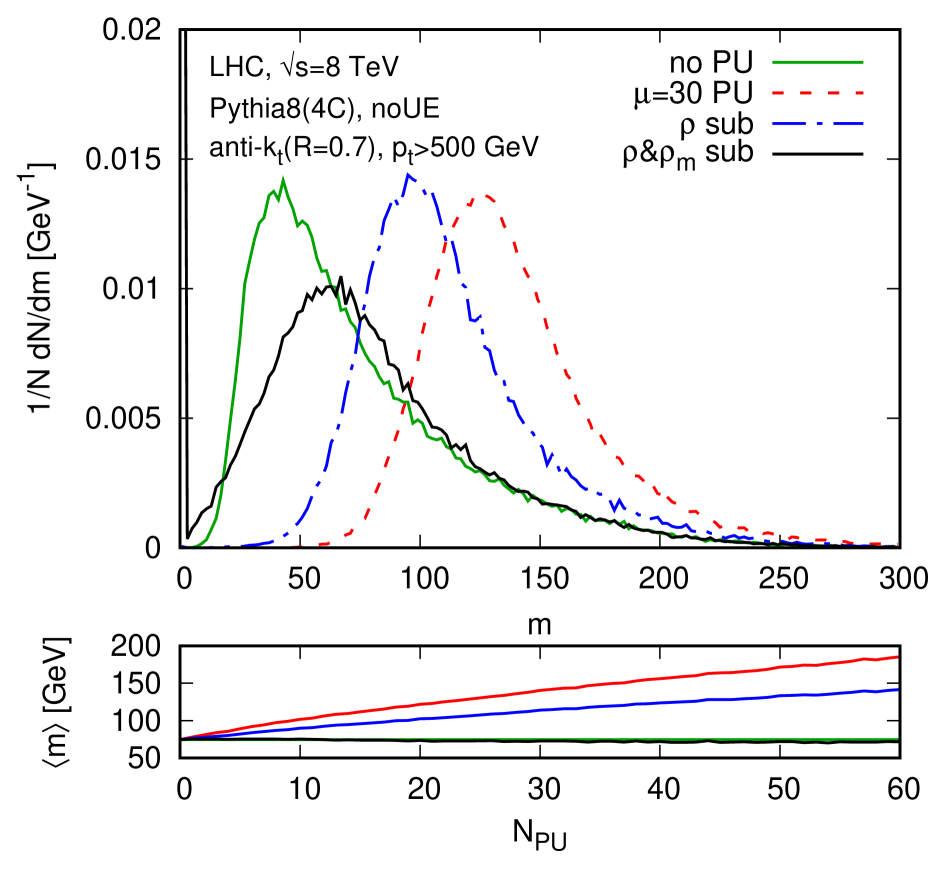
Let us first briefly discuss the subtraction of the jet mass and the necessity to include the $\rho_{m}$ term in (2.30) when particles are massive. This is illustrated on Fig. 3.14 where we have measured the jet-mass spectrum for anti-$k_{t}(R=0.7)$ jets with $p_{t}>500$ GeV, together with the shift of the average mass as a function of $N_{\mathrm{PU}}$ on the lower panel. Compared to the distribution observed without pileup (the solid green line), we see that adding pileup (dashed red line) significantly shifts the distribution to larger masses. If we apply the area–median subtraction Eq. (2.24), the dash-dotted line in Fig. 3.14, we still observe a large mass shift. Only once we also include the $\rho_{m}$ correction do we recover the right average mass, explicitly proving the importance of that correction with massive particles.

It is also interesting to notice that the mass peak is not quite well reproduced at small jet masses. In that region, the jet mass is rather sensitive to pileup fluctuations resulting in a smeared peak.

We now turn to the validation of the pileup subtraction method for jet shapes introduced in Section 2.5. To investigate the performance of our correction procedure, we consider a number of jet shapes:

• Angularities [65, 66], adapted to hadron-collider jets as $\theta^{(\beta)}=\sum_{i}p_{ti}\Delta R_{i,\mathrm{jet}}^{\beta}/\sum_{i}p_{ti}$, for $\beta=0.5,1,2,3$; $\theta^{(1)}$, the “girth”, “width” or “broadening” of the jet, has been found to be particularly useful for quark/gluon discrimination [67, 68].

• Energy-energy-correlation (EEC) moments, advocated for their resummation simplicity in [69], $E^{(\beta)}=\sum_{i,j}p_{ti}p_{tj}\Delta R_{i,j}^{\beta}/(\sum_{i}p_{ti})^{2}$, using the same set of $\beta$ values. EEC-related variables have been studied recently also in Refs.[70, 71, 72].

• “Subjettiness” ratios, designed for characterising multi-pronged jets [73, 74, 75]: one defines the subjettiness $\tau_{N}^{(\text{axes},\beta)}=$ $\sum_{i}p_{ti}\min(\Delta R_{i1},\ldots,\Delta R_{iN})^{\beta}/\sum_{i}p_{ti}$, where $\Delta R_{ia}$ is the distance between particle $i$ and axis $a$, where $a$ runs from $1$ to $N$. One typically considers ratios such as $\tau_{21}\equiv\tau_{2}/\tau_{1}$ and $\tau_{32}\equiv\tau_{3}/\tau_{2}$ (the latter used e.g. in a recent search for R-parity violating gluino decays [76]); we consider $\beta=1$ and $\beta=2$, as well as two choices for determining the axes: “kt”, which exploits the $k_{t}$ algorithm to decluster the jet to $N$ subjets and then uses their axes; and “1kt”, which adjusts the “kt” axes so as to obtain a single-pass approximate minimisation of $\tau_{N}$ [75].

• A longitudinally invariant version of the planar flow [77, 66], involving a $2\times 2$ matrix $M_{\alpha\beta}=\sum_{i}p_{ti}(\alpha_{i}-\alpha_{\text{jet}})(\beta_{i}-\beta_{\text{jet}})$, where $\alpha$ and $\beta$ correspond either to the rapidity $y$ or azimuth $\phi$; the planar flow is then given by $\text{Pf}=4\lambda_{1}\lambda_{2}/(\lambda_{1}+\lambda_{2})^{2}$, where $\lambda_{1,2}$ are the two eigenvalues of the matrix.

One should be aware that observables constructed from ratios of shapes, such as $\tau_{n,n-1}$ and planar flow, are not infrared and collinear (IRC) safe for generic jets. In particular Pf and $\tau_{21}$ are IRC safe only when applied to jets with a structure of at least two hard prongs, usually guaranteed by requiring the jets to have significant mass; $\tau_{32}$ requires a hard three-pronged structure, a condition not imposed in previous work, and that we will apply here through a cut on $\tau_{21}$.

For the angularities and EEC moments we have verified that the first two numerically-obtained derivatives agree with analytical calculations in the case of a jet consisting of a single hard particle. For variables like $\tau_{N}$ that involve a partition of a jet, one subtlety is that the partitioning can change as the ghost momenta are varied to evaluate the numerical derivative. The resulting discontinuities (or non-smoothness) in the observable’s value would then result in nonsensical estimates of the derivatives. We find no such issue in our numerical method to evaluate the derivatives, but were it to arise, one could choose to force a fixed partitioning.

To test the method in simulated events with pileup, we use Pythia 8.165, tune 4C. We consider 3 hard event samples: dijet, $WW$ and $t\bar{t}$ production, with hadronic $W$ decays, all with underlying event (UE) turned off (were it turned on, the subtraction procedure would remove it too). We use anti-$k_{t}$ jets with $R=0.7$, taking only those with $p_{t}>500\,\mathrm{GeV}$ (before addition of pileup). All jet-finding is performed with FastJet 3.0. The determination of $\rho$ and $\rho_{m}$ for each event follows the area–median approach using Eqs. (2.23) and (2.29) to estimate the background properties and (2.30) to correct the jet 4-momentum. Here, the estimation of $\rho$ and $\rho_{m}$ is done using jets obtained with the $k_{t}$ algorithm with $R=0.4$ and includes rapidity rescaling.

Figure 3.15: Impact of pileup and subtraction on various jet-shape distributions and their averages, in dijet, $WW$ and $t\bar{t}$ production processes. The distributions are shown for Poisson distributed pileup (with an average of $30$ pileup events) and the averages are shown as a function of the number of pileup events, ${N_{\mathrm{PU}}}$. The shapes are calculated for jets with $p_{t}>500\,\mathrm{GeV}$ (the cut is applied before adding pileup, as are the cuts on the jet mass $m_{J}$ and subjettiness ratio $\tau_{21}$ where relevant).

Figure 3.16: Left: rate for tagging quark and gluon jets using a fixed cut on the jet width, shown as a function of the number of pileup vertices. Middle: filtered jet-mass distribution for fat jets in $t\bar{t}$ events, showing the impact of the $\rho$ and $\rho_{m}$ components of the subtraction. Right: tagging rate of an $N$-subjettiness top tagger for $t\bar{t}$ signal and dijet background as a function of the number of pileup vertices. All cuts are applied after addition (and possible subtraction) of pileup. Subtraction acts on $\tau_{1}$, $\tau_{2}$ and $\tau_{3}$ individually. See text for further details.

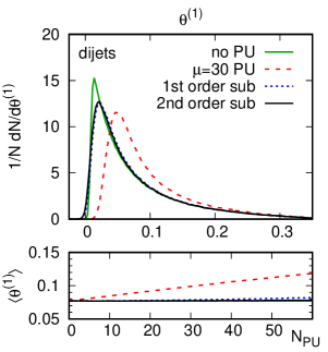
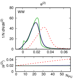
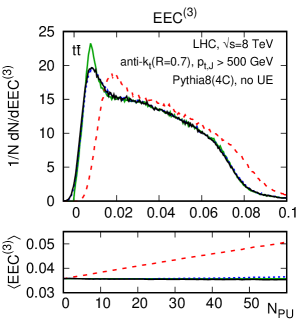
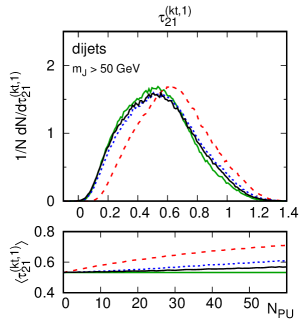
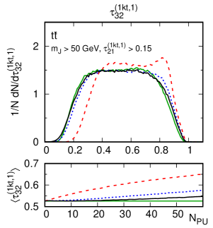
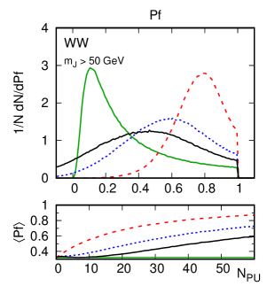
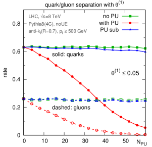
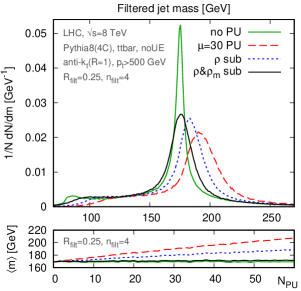
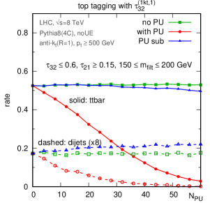
We have 17 observables and 3 event samples. Fig. 3.15 gives a representative subset of the resulting $51$ distributions, showing in each case both the distribution (top panel) and average shift (bottom panel, plotted as function of $N_{\mathrm{PU}}$) for the shape without pileup (solid green line), the result with pileup (dashed line) and the impact of subtracting first and second derivatives (dotted and solid black lines respectively). The plots for the distributions have been generated using a Poisson distribution of pileup events with an average of $\mu=30$ events.

For nearly all the jet shapes, the pileup has a substantial impact, shifting the average values by up to $50-100\%$ (as compared to a $5-10\%$ effect on the jet $p_{t}$). The subtraction performs adequately: the averaged subtracted results for the shapes usually return very close to their original values, with the second derivative playing a small but sometimes relevant role. For the distributions, tails of the distributions are generally well recovered; however intrajet pileup fluctuations cause sharp peaks to be somewhat broadened. These cannot be corrected for without applying some form of noise reduction, which would however also tend to introduce a bias. Of the 51 combinations of observable and process that we examined, most were of similar quality to those illustrated in Fig. 3.15, with the broadening of narrow peaks found to be more extreme for larger $\beta$ values. The one case where the subtraction procedure failed was the planar flow for (hadronic) $WW$ events: here the impact of pileup is dramatic, transforming a peak near the lower boundary of the shape’s range, $\text{Pf}=0$, into a peak near its upper boundary, $\text{Pf}=1$ (bottom-right plot of Fig. 3.15). This is an example where one cannot view the pileup as simply “perturbing” the jet shape, in part because of intrinsic large non-linearities in the shape’s behaviour; with our particular set of $p_{t}$ cuts and jet definition, the use of the small-$\rho$ expansion of Eq. (2.33) fails to adequately correct the planar flow for more than about $15$ pileup events.

Next, we want to show the behaviour of the area–median subtraction for jet shapes in more practical applications.

We first consider the use of the subtraction approach in the context of quark/gluon discrimination. In a study of a large number of shapes, Ref. [67] found the jet girth or broadening, $\theta^{(1)}$, to be the most effective single infrared and collinear safe quark/gluon discriminator. Fig. 3.16 (left) shows the fraction of quark and gluon-induced jets that pass a fixed cut on $\theta^{(1)}\leq 0.05$ as a function of the level of pileup — pileup radically changes the impact of the cut, while after subtraction the q/g discrimination returns to its original behaviour.

Our last test involves top tagging, which we illustrate on $R=1$, anti-$k_{t}$ jets using cuts on the “filtered” jet mass and on the $\tau_{32}$ subjettiness ratio. The filtering selects the 4 hardest $R_{\text{filt}}=0.25$, Cambridge/Aachen subjets after pileup subtraction. The distribution of filtered jet mass is shown in Fig. 3.16 (middle), illustrating that the subtraction mostly recovers the original distribution and that $\rho_{m}$ is as important as $\rho$ (specific treatments of hadron masses, e.g. setting them to zero, may limit the impact of $\rho_{m}$ in an experimental context). The tagger itself consists of cuts on $\tau_{32}<0.6$, $\tau_{21}\geq 0.15$ and a requirement that the filtered [79] jet mass be between $150$ and $200$ GeV. The rightmost plot of Fig. 3.16 shows the final tagging efficiencies for hadronic top quarks and for generic dijets as a function of the number of pileup events. Pileup has a huge impact on the tagging, but most of the original performance is restored after subtraction.

Chapter 4 Applications to heavy-ion collisions

In this Chapter, we shall review the performance of the area–median subtraction method applied to heavy-ion collisions.

Prior to any physics discussion, we should mention that the Monte Carlo studies presented in this Chapter were made before any heavy-ion collision actually happened at the LHC, at a time where jet reconstruction in such a busy environment was still in its early days.

Our studies mostly correspond to $\sqrt{s}=5.5$ TeV, except for the jet fragmentation studies presented in Section 4.7 where we have used $\sqrt{s}=2.76$ TeV. Since no LHC data were available at the time of our study, the Monte Carlo generators we used to simulate $PbPb$ collision had to be extrapolated from RHIC energies. In practice, it seems that the tunes we have adopted are doing a decent job at capturing what is now known from LHC data. This is at the very least good enough for the purpose of the indicative studies in this Chapter and we have not deemed necessary to update our results to the lower centre-of-mass energy or to more modern generators and tunes. A discussion comparing the tune we used for $\sqrt{s}=2.76$ TeV collisions and first LHC measurements can be found in Ref. [80].

4.1 Challenges of jet reconstruction in heavy-ion collisions

Jets in HI collisions are produced in an environment that is far from conducive to their detection and accurate measurement. Monte Carlo simulations (and real RHIC data) for gold–gold collisions at $\sqrt{s_{NN}}=200$ GeV (per nucleon–nucleon collision) show that the transverse momentum density $\rho$ of final-state particles is about 100 GeV per unit area (in the rapidity–azimuth plane). For lead–lead collisions at $\sqrt{s_{NN}}=2.36$ TeV or $5.5$ TeV at the LHC this figure was expected to increase by some factor $\sim 2{-}3$. This means that jets returned by jet definitions with a radius parameter of, e.g. , $R=0.4$, will contain background contamination of the order of $\pi R^{2}\rho\simeq$ 50 and $100-150\,\mathrm{GeV}$ respectively.

A related, and perhaps more challenging obstacle to accurate jet reconstruction is due to the fluctuations both of the background level (from event to event, but also from point to point in a single event) and of the jet area itself: knowing the contamination level ‘on average’ is not sufficient to accurately reconstruct each individual jet.

Our framework has the following characteristics:

• We shall consider a wider range of jet algorithms, still restricting ourselves to IRC safe algorithms. In particular, the jet algorithms we use will not be limited to those yielding jets of regular shape. This point probably has to be put in the historical context: at the time we conducted this study, the LHC had not taken any $PbPb$ data and jet reconstruction in heavy-ion collisions was still in its infancy. Opening our study to a variety of jet algorithms is meant to provide a broader perspective on the topic. We shall see that it indeed comes with a few interesting observations.

• Our analysis will avoid excluding small transverse momentum particles from the clustering as some original approaches were leaning towards. Doing so is collinear-unsafe and inevitably biases the reconstructed jet momenta, which must then be corrected using Monte Carlo simulations, which can have substantial uncertainties in their modelling of jet quenching and energy loss. Instead, we shall try to achieve a bias-free reconstructed jet, working with all the particles in the event.

• The analysis presented here was achieved before the grid-based approach to estimating $\rho$ was introduced and before rescaling was suggested to correct for positional dependence of $\rho$. The study presented below will therefore be limited to jet-based estimates of $\rho$, with local ranges to control the positional dependence. This is however perfectly sufficient to illustrate our the points we want to make. Unpublished preliminary studies show that similar performance can be reached with rapidity rescaling. In particular a rescaling in $\phi$ can be used to handle the elliptic flow. We will not include these results here.

Some of the features observed here are also closely connected to some analytic considerations discussed in the next Chapter of this document.

4.2 Details of the study

4.2.1 Simulation and analysis framework

Embedding.

As for the $pp$ study from Section 3.2 above, we shall proceed by embedding a “truth” hard jet in a heavy-ion background and study how precisely area–median subtraction corrects the jets back to their truth.

This approach is however less motivated in the case of heavy-ion collisions where the physical separation between the jets and the heavy-ion Underlying Event (HI-UE) is not well-defined as it was the case for pileup in $pp$ collisions. This is due to the intrinsic interaction between the products of the “hard” collision and the dense heavy-ion medium it travels through. In today’s Monte-Carlo event generators for heavy-ion collisions, such a separation is however possible and we shall use that to gain some knowledge of how efficient the area–median subtraction subtracts that unwanted contribution. In that context, it is important to check that our conclusions are not affected neither by the details of the HI-UE, nor by the details of the embedded hard jets, including the fact that they are quenched of not. In that context, the subtraction procedure can be seen as directly belonging to our definition of jets.

In practice, if the Monte Carlo program used to simulate heavy-ion events explicitly provides a separation between hard events and a soft part — e.g. as does Hydjet [81, 82] — one can extract one of the former as the single hard event and take the complete event as the full one. Alternatively, one can generate a hard event independently and embed it in a heavy-ion event (obtained from a Monte Carlo or from real collisions) to obtain the full event. This second approach, which we have adopted for the bulk of results presented here because of its greater computational efficiency, is sensible as long as the embedded hard event is much harder than any of the semi-hard events that tend to be present in the background. For the transverse momenta that we consider, this condition is typically fulfilled. Note however that for studies in which the presence of a hard collision is not guaranteed, e.g. the evaluation of fake-jet rates discussed below, one should use the first approach.

Matching and quality measures.

We shall use the same procedure as for our earlier study of the jet $p_{t}$ in $pp$ collisions, Namely, we will reconstruct the jets in both the hard and the full events, — yielding the “hard” and “full” jets — apply the kinematic cuts on the hard jets to guarantee a clean sample, and consider a full jet as matched to a hard jet if their shared constituents make up at least 50% of the transverse momentum of the constituents of the hard jet. Events without any matched jets are simply discarded and contribute to the evaluation of matching inefficiencies (see section 4.3.1). For what follows, we shall keep only the pairs of jets which have been matched to one of the two hardest (subtracted) jets in the hard event.

For a matched pair of jets we can compute the corresponding shift $\Delta p_{t}$ as introduced in Eq. (3.5). We shall mostly focus our study on same two quality measures used in Section. 3.2: the average $p_{t}$ shift, $\langle\Delta p_{t}\rangle$, and its dispersion, $\sigma_{\Delta p_{t}}\equiv\sqrt{\left\langle\Delta p_{t}^{2}\right\rangle-\left\langle\Delta p_{t}\right\rangle^{2}}$, where the average is made over the events. Small (absolute) values of both $\left\langle\Delta p_{t}\right\rangle$ and $\sigma_{\Delta p_{t}}$ will be the sign of a good subtraction.

Monte Carlo simulations.

Quantifying the quality of background subtraction using Monte Carlo simulations has several advantages. Besides providing a practical way of generating the hard “signal” separately from the soft background, one can easily check the robustness of one’s conclusions by changing the hard jet or the background sample.

One difficulty that arises in gauging the quality of jet reconstruction in heavy-ion collisions comes from the expectation that parton fragmentation in a hot medium will differ from that in a vacuum. This difference is often referred to as jet quenching [83, 84] (for reviews, see e.g.  [85, 86, 87, 88]). The details of jet quenching are far less well established than those of vacuum fragmentation and can have an effect on the quality of jet reconstruction. Here we shall examine the reconstruction of both unquenched and quenched jets. For the latter it will be particularly important to be able to test more than one quenching model, in order to help build confidence in our conclusions about any reconstruction bias that may additionally exist in the presence of quenching.

In practice, for this study we have used both the Fortran (v1.6) [81] and the C++ (v2.1) [82] versions of Hydjet to generate the background. Hard jets have been generated with Pythia 6.4 [89, 90, 91], either running it standalone, or using the version embedded in Hydjet v1.6.. The quenching effects have been studied using both QPythia [92, 93] and Pyquen [81, 94].

4.2.2 Jet reconstruction: definition and subtraction

Jet definitions.

Since jet reconstruction in heavy-ion collisions is far more complex than in the $pp$ case, we shall widen a bit our perspective and consider a series of jet definitions. This will also allow us to highlight some of the key differences between the algorithms, in particular in their response to soft backgrounds.

We shall therefore use the $k_{t}$, Cambridge/Aachen (C/A), and anti-$k_{t}$ algorithms. In an attempt to further reduce the sensitivity of the jets to soft backgrounds, we have also investigated grooming techniques (see the next part of this document for more on this topic). In practice, we have considered “filtering” [79] which works by reclustering each jet with a radius $R_{\rm filt}$ smaller than the original radius $R$ and keeping only the $n_{\rm filt}$ hardest subjets (see also Chapter 6). Background subtraction is applied to each of the subjets before deciding which ones to keep. In this study, we have used filtering applied to Cambridge/Aachen (C/A(filt)) with $R_{\rm filt}=R/2$ and $n_{\rm filt}=2$. We have not used SISCone, as its relatively slower speed compared to the sequential recombination algorithms makes it less suitable for a HI environment.

In all cases, we have taken the radius parameter $R=0.4$. We have adopted this value as it is the largest used at RHIC and a reasonable choice for the LHC. Note that the effect of the background fluctuations of the jet energy resolution increases linearly with $R$, disfavouring significantly larger choices. On the other hand, too small a choice of $R$ may lead to excessive sensitivity to the details of parton fragmentation, hadronisation and detector granularity.

Background determination and subtraction.

This will be carried using the now familiar area–median approach. The background density $\rho$ will be obtained from a jet-based estimation and the choice of an algorithm and a jet radius $R_{\rho}$ will be discussed below.

To handle the positional dependence, we shall use the local range technique. Besides the global estimate of $\rho$, independent of the jet position, we shall consider three options for a local range introduced in Section 2.4.2: the strip range ${\cal S}_{\Delta}(j)$, the circular range ${\cal C}_{\Delta}(j)$, and the doughnut range ${\cal D}_{\delta,\Delta}(j)$. Whenever this is necessary, we shall denote by ${\cal R}(j)$ a range around jet $j$.

When using a local range, a compromise needs to be found between choosing a range small enough to get a valid local estimation, but also large enough to contain a sufficiently large number of background (soft) jets for the estimation of the median to be reliable. Two effects need to be considered: (1) statistical fluctuations in the estimation of the background and (2) biases due to the presence of a hard jet in the region used to estimate the background.

1. If we require that the dispersion in the reconstructed jet $p_{t}$ coming from the statistical fluctuations in the estimation of the background (Eq. (5.103) multiplied by the area of the jet) does not amount to more than a fraction $\epsilon$ of the overall $\sigma_{\Delta p_{t}}\approx\sigma\sqrt{A_{\rm jet}}$, then — see Section 4.4.4 for details — the range needs to cover an area $A_{\cal R}$ such that

   $$A_{\cal R}\gtrsim\frac{\pi^{2}R^{2}}{4\epsilon}\,.$$ (4.1)

   Taking $\epsilon=0.1$ and $R=0.4$ this corresponds to an area $A_{\cal R}\gtrsim 25R^{2}\simeq 4$. For the applications below, when clustering with radius $R$, we have used the rapidity-strip ranges ${\cal S}_{2R}$ and ${\cal S}_{3R}$, the circular range ${\cal C}_{3R}$ and the doughnut range ${\cal D}_{R,3R}$. One can check that their areas are compatible with the $25R^{2}$ lower-limit estimated above.

2. The bias in the estimate of $\rho$ due to the presence of $n_{b}$ hard jets in the range is given roughly by

   $$\langle\Delta\rho\rangle\simeq 1.8\sigma R_{\rho}\frac{n_{b}}{A_{\cal R}}\,,$$ (4.2)

   as discussed in Section 4.4.5. The ensuing bias on the $p_{t}$ can be estimated as $\langle\Delta\rho\rangle\pi R^{2}$ (for anti-$k_{t}$ jets). For $R=0.4$, $R_{\rho}=0.5$, $A_{\cal R}\simeq 4$ and $n_{b}=1$, the bias in the reconstructed jet $p_{t}$ is $\simeq 0.1\sigma$. Given $\sigma$ in the $10-20\,\mathrm{GeV}$ range (as we will find in section 4.3) this corresponds to a $1-2\,\mathrm{GeV}$ bias. In order to eliminate this small bias, we will often choose to exclude the two hardest jets in each event when determining of $\rho$.

A third potential bias discussed in ref. [37] is that of underestimating the background when using too small a value for $R_{\rho}$. Given the high density of particles in HI collisions, this will generally not be an issue as long as $R_{\rho}\sim 0.5$.

4.3 Results

Figure 4.1: Distribution of the background density $\rho$ per unit area (left) and its intra-event fluctuations $\sigma$ (right). It has been obtained from 5000 Hydjet events with RHIC (AuAu, $\sqrt{s_{NN}}=200\,\mathrm{GeV}$) and LHC (PbPb, $\sqrt{s_{NN}}=5.5\,\mathrm{TeV}$) kinematics. The background properties have been estimated using the techniques presented in section 4.2.2, using the $k_{t}$ algorithm with $R_{\rho}=0.5$, and keeping only the jets with $|y|<1$ (excluding the two hardest).

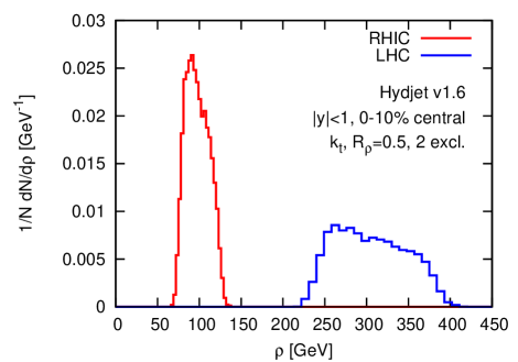
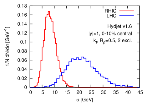
Let us first discuss the main characteristics of the background properties. Our setup for the background, using Hydjet v1.6 with 0-10% centrality leads, for RHIC (AuAu, $\sqrt{s_{NN}}=200\,\mathrm{GeV}$), to an average background density per unit area at central rapidity of $\langle\rho\rangle\simeq 99$ GeV with average fluctuations in a single event of $\langle\sigma\rangle\simeq 8$ GeV and event-to-event fluctuations $\sigma_{\rho}\equiv\sqrt{\langle\rho^{2}\rangle-\langle\rho\rangle^{2}}\simeq 14$ GeV. For the LHC (PbPb, $\sqrt{s_{NN}}=5.5\,\mathrm{TeV}$) the corresponding values are $\langle\rho\rangle\simeq 310$ GeV, $\langle\sigma\rangle\simeq 20$ GeV and event-to-event fluctuations $\sigma_{\rho}\simeq 45$ GeV. Fig. 4.1 shows the distributions obtained from the simulations for $\rho$ and $\sigma$.

In the case of the RHIC simulation, the result for $\left\langle\rho\right\rangle$ is somewhat higher than the experimental value of $75\,\mathrm{GeV}$ quoted by the STAR collaboration [96, 97], however this is probably in part due to limited tracking efficiencies at low $p_{t}$ at STAR, and explicit STAR [98] and PHENIX [99] results for $dE_{t}/d\eta$ correspond to somewhat higher $\rho$ values, about $90\,\mathrm{GeV}$. The multiplicity of charged particles ($dN_{ch}/d\eta\simeq 660$ for $\eta=0$ and 0–6% centrality) and the pion $p_{t}$ spectrum in our simulation are sensible compared to experimental measurements at RHIC [100, 101, 102]. For the LHC our charged particle multiplicity is $dN_{ch}/d\eta\simeq 1600$ for $\eta=0$ and 0–10% centrality, which is comparable to many of the predictions reviewed in fig. 7 of [103].

An independent control analysis has also been performed with Hydjet++ 2.1 [82] (with default parameters) for the background. The results at RHIC are similar, while for LHC the comparison is difficult because the default tune of Hydjet++ 2.1 predicts a much higher multiplicity, $dN_{ch}/d\eta\simeq 2800$ for $\eta=0$ and 0–10% centrality.

Most of the results of this section will be obtained without quenching, though in section 4.3.5 we will also consider the impact on our conclusions of the Pyquen and QPythia simulations of quenching effects.

For the results presented below, we have employed a selection cut of $|y|\leq y_{\rm max}$ on the jets with $y_{\rm max}=1$ for RHIC and $y_{\rm max}=2.4$ for the LHC. We only consider full jets that are matched to one of the two hardest jets in the hard event. The computation of the jet areas in FastJet, needed both for the subtraction and the background estimation, has been performed using active areas (including explicit ghosts), with ghosts up to $y_{\rm max}+1.8$, a single repetition and a ghost area of 0.01.The determination of the background density $\rho$ has been performed using the $k_{t}$ algorithm with $R_{\rho}=0.5$. Though the estimate of the background depends on $R_{\rho}$ [37] (see also Section 5.2), we have observed that choices between 0.3 and 0.5 lead to very similar results (e.g. differing by at most a few hundred MeV at RHIC).

4.3.1 Matching efficiency

Figure 4.2: Matching efficiency for reconstructed jets as a function of the jet $p_{t}$. Left: RHIC, right: LHC. These results are independent of the choice of background-subtraction range in the heavy-ion events, since background subtraction does not enter into the matching criterion. Here and in later figures, the label “unquenched” refers to the embedded $pp$ event; the background is always simulated including quenching.

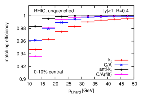
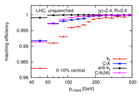
Let us start the presentation of our results with a brief discussion of the efficiency of reconstructing jets in the medium. As explained in Section 4.2.1, the jets in the medium are matched to a “bare” hard jet when their common particle content accounts for at least 50% of the latter’s transverse momentum.

The matching efficiencies we observe depend to some extent on the details of the Monte Carlo used for the background so our intention is just to illustrate the typical behaviour we observe and highlight that these efficiencies tend to be large. We observe from fig. 4.2 that we successfully match at least 95% of the jets above $p_{t}\simeq 15$ GeV at RHIC, and at least 99% of the jets above $p_{t}\simeq 60$ GeV at the LHC. It is also interesting to notice that the anti-$k_{t}$ algorithm performs best, likely as a consequence of its ‘rigidity’, namely the fact that anti-$k_{t}$ jets tend to have the same (circular) shape, independently of the soft-particles that are present.

4.3.2 Choice of background-estimation range

Figure 4.3: Effect of the choice of range on the average $p_{t}$ shift, $\Delta p_{t}$, as defined in Eq. (3.5). Left: RHIC, right: LHC. In this figure and those that follow, the yellow band corresponds to 1% of the $p_{t}$ of the hard jet.

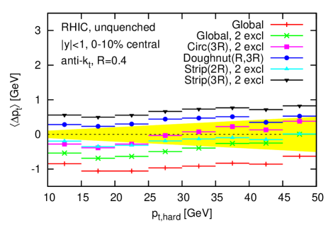
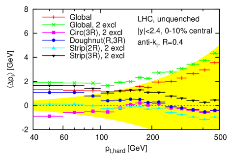
We now turn to the results concerning the measurement of the background density and the reconstruction of the jet transverse momentum. We first concentrate on the impact of the choice of a local range and/or of the exclusion of the two hardest jets when determining $\rho$.

In fig. 4.3 we show the average shift $\left\langle\Delta p_{t}\right\rangle$ for the list of ranges mentioned in section 4.2.2. The results presented here have been obtained with the anti-$k_{t}$ algorithm with $R=0.4$, but the differences among the various range choices have been seen to be similar with other jet definitions. The label “2 excl” means that the two hardest jets in the event have been excluded from the estimation of the background. We have found that this improves the precision of the subtractions whenever expected, i.e. for all choices of range except the doughnut range, where its central hole already acts similarly to the exclusion of the hardest jets. To keep the figure reasonably readable, we have only explicitly shown the effect of removing the two hardest jets for the global range. The change of 0.4–0.6 GeV (both for RHIC and the LHC) is in reasonable agreement with the analytic estimate of about 0.6 GeV for RHIC and the LHC obtained from $\left\langle\Delta p_{t}\right\rangle=\pi R^{2}\left\langle\Delta\rho\right\rangle$ with $\left\langle\Delta\rho\right\rangle$ calculated using Eq. (4.2). Note that at LHC the exclusion of the two hardest jets for the global range appears to worsen the subtraction, however what is really happening is that the removal of the two hardest jets exacerbates a deficiency of the global range, namely the fact that its broad rapidity coverage causes it to underestimate $\rho$, leading to a positive net $\left\langle\Delta\rho\right\rangle$.

Other features that can be understood qualitatively include for example the differences between the two strip and the global (2 excl) range for RHIC: while the rapidity width of the global range lies in between that of the two strip ranges, the global range gives a lower $\left\langle\Delta p_{t}\right\rangle$ than both, corresponding to a larger $\rho$ estimate, which is reasonable because the global range is centred on $y=0$, whereas the strip ranges are mostly centred at larger rapidities where the background is lower.

The main result of the analysis of fig. 4.3 is the observation that all choices of a local range lead to a small residual $\Delta p_{t}$ offset: the background subtraction typically leaves a $|\left\langle\Delta p_{t}\right\rangle|\lesssim 1\,\mathrm{GeV}$ at both RHIC and LHC, i.e. better than 1-2% accuracy over much of the $p_{t}$ range of interest. It is not clear, within this level of accuracy, if one range is to be preferred to another, nor is it always easy to identify the precise origins of the observed differences between various ranges. Another way of viewing this is that the observed differences between the various choices give an estimate of the residual subtraction error due to possible misestimation of $\rho$. For our particular analysis, at RHIC this comment also applies to the choice of the global range (with the exclusion of the two hardest jets in the event). This is a consequence of the limited rapidity acceptance, which effectively turns the global range into a local one, a situation that does not hold for larger rapidity acceptances, as we have seen for the LHC results. In what follows we will use the Doughnut($R,3R$) choice, since it provides a good compromise between simplicity and effectiveness.

4.3.3 Choice of algorithm

Figure 4.4: Distribution of $\Delta p_{t}$ (red histograms) for each of our 4 jet algorithms, together with a Gaussian (black curve) whose mean (solid vertical line) and dispersion are equal to $\left\langle\Delta p_{t}\right\rangle$ and $\sigma_{\Delta p_{t}}$ respectively.

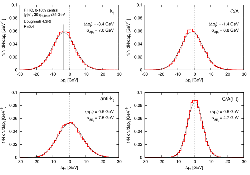
The next potential systematic effect that we consider is the choice of the jet algorithm used for the clustering. Fig. 4.4 shows the distribution of $\Delta p_{t}$ for each of our four choices of jet algorithm, $k_{t}$, C/A, anti-$k_{t}$ and C/A(filt), given for RHIC collisions and a specific bin of the hard jets’ transverse momenta, $30<p_{t,\text{hard}}<35\,\mathrm{GeV}$. One sees significant differences between the different algorithms. One also observes that Gaussians with mean and dispersion set equal to $\left\langle\Delta p_{t}\right\rangle$ and $\sigma_{\Delta p_{t}}$ provide a fair description of the full histograms. This validates our decision to concentrate on $\left\langle\Delta p_{t}\right\rangle$ and $\sigma_{\Delta p_{t}}$ as quality measures. One should nevertheless be aware that in the region of high $|\Delta p_{t}|$ there are deviations from perfect Gaussianity, which are more visible if one replicates fig. 4.4 with a logarithmic vertical scale (not shown, for brevity).

Average $\Delta p_{t}$.

Figure 4.5: Average shift $\left\langle\Delta p_{t}\right\rangle$, as a function of $p_{t,\text{hard}}$, shown for RHIC (left) and the LHC (right).

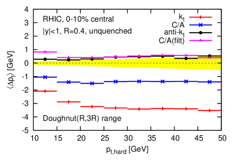
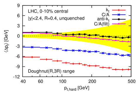
The first observable we analyse is the average $p_{t}$ shift. We show in fig. 4.5 the $\langle\Delta p_{t}\rangle$ results for the four algorithms listed in Section 4.2.2, as a function of $p_{t,\text{hard}}$. We use the doughnut range to estimate the background. The first observation is that, while the anti-$k_{t}$ and C/A(filt) algorithms have a small residual $\left\langle\Delta p_{t}\right\rangle$, the C/A and $k_{t}$ algorithms display significant offsets. The reason for the large offsets of $k_{t}$ and C/A is well understood, related to the effect of back-reaction. This is the fact that the addition of a soft background can alter the clustering of the particles of the hard event: some of the constituents of a jet in the hard event can be gained by or lost from the jet when clustering the event with the additional background of the full event. This happens, of course, on top of the simple background contamination that adds background particles to the hard jet. Even if this latter contamination is subtracted exactly, the reconstructed $p_{t}$ will still differ from that of the original hard jet as a consequence of the back-reaction.

Figure 4.6: Contribution to $\left\langle\Delta p_{t}\right\rangle$ due to back-reaction. Note that these results are independent of the range used for estimating $\rho$ in the heavy-ion event. Left: RHIC, right: LHC.

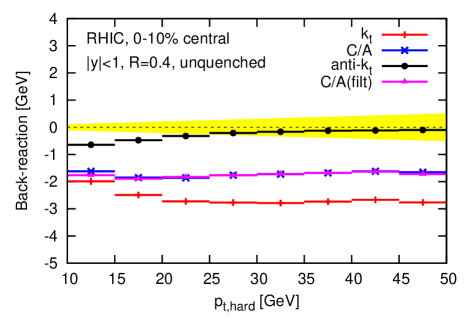
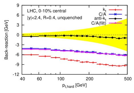
The effect of the back-reaction can be studied in detail, since in Monte Carlo simulations it is possible to identify which hard-event constituents are present in a given jet before and after inclusion of the background particles in the clustering. The average $p_{t}$ shift due to back-reaction can be seen in fig. 4.6 for the different jet algorithms. As expected (see Section 5.1.3 or Refs. [41, 29], it is largest for $k_{t}$, and smallest (almost zero, in fact) for anti-$k_{t}$. By comparing fig. 4.6 and fig. 4.5 one can readily explain the difference between the $\left\langle\Delta p_{t}\right\rangle$ offsets of the various algorithms in terms of their back-reaction. The rigidity (and hence small back-reaction) of the anti-$k_{t}$ jets manifestly gives almost bias-free reconstructed jets, while the large back-reaction effects of the $k_{t}$ algorithm and, to a smaller extent, of the C/A algorithm translates into a worse performance in terms of average shift. The $p_{t}$ dependence of the back-reaction is weak. This is expected based on the interplay between the $\ln\ln p_{t}$ dependence found in Section 5.1.3 [29] and the evolution with $p_{t}$ of the relative fractions of quark and gluon jets.

The case of the C/A(filt) algorithm is more complex: its small net offset, comparable to that of the anti-$k_{t}$ algorithm, appears to be due to a fortuitous compensation between an under-subtraction of the background and a negative back-reaction. The negative back-reaction is very similar to that of C/A without filtering, while the under-subtraction is related to the fact that the selection of the hardest subjets introduces a bias towards positive fluctuations of the background. This effect is discussed in Section 4.4.6, where we obtain the following estimate for the average $p_{t}$ shift (specifically for $R_{\rm filt}=R/2$):

$$\left\langle(\Delta p_{t})_{\rm filt}\right\rangle\simeq 0.56\,R\sigma,$$ (4.3)

yielding an average bias of 2 GeV for RHIC and 4.5 GeV at the LHC, which are both in good agreement with the differences observed between C/A with and without filtering in fig. 4.5. Note that while the bias in Eq. (4.3) is proportional to $\sigma$, the back-reaction bias is instead mainly proportional to $\rho$. It is because of these different proportionalities that the cancellation between the two effects should be considered as fortuitous. Since it also depends on the substructure of the jet, one may also expect that the cancellation that we see here could break down in the presence of quenching.

Dispersion of $\Delta p_{t}$.

Figure 4.7: Dispersion $\sigma_{\Delta p_{t}}$. Left: RHIC, right: LHC.

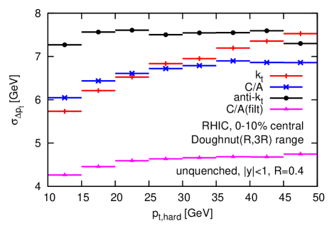
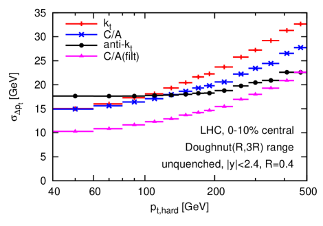
Our results for the $\Delta p_{t}$ dispersion, $\sigma_{\Delta p_{t}}$, are shown in fig. 4.7, again using the doughnut range. (Our conclusions are essentially independent of the particular choice of range.)

We first discuss the case of RHIC kinematics. For $k_{t}$ and anti-$k_{t}$, the observed dispersions are similar to the result of $6.8\,\mathrm{GeV}$ quoted by STAR [96, 97] (though the number from STAR includes detector resolution effects, so that the true physical $\sigma_{\Delta p_{t}}$ may actually be somewhat lower). Of note, the advantage enjoyed by anti-$k_{t}$ in terms of smallest $\left\langle\Delta p_{t}\right\rangle$ does not hold at the level of the dispersion: C/A and $k_{t}$ tend to behave slightly better at small transverse momentum. The algorithm which performs best in terms of dispersion over all the $p_{t}$ range is now C/A with filtering, for which the result is smaller than that of the other algorithms by a factor of about $1/\sqrt{2}$. This reduction factor can be explained because the dispersion $\sigma_{\Delta p_{t}}$ is expected to be proportional to the square-root of the jet area: the C/A(filt) algorithm with $R_{\rm filt}=R/2$ and $n_{\rm filt}=2$ produces jets with an area of, roughly, half that obtained with C/A; hence the observed reduction of $\sigma_{\Delta p_{t}}$.

In the LHC setup, the conclusions are quite similar at the lowest transverse momenta shown. As $p_{t}$ increases, the dispersion of the anti-$k_{t}$ algorithm grows slowly, while that of the others grows more rapidly, so that at the highest $p_{t}$’s shown, the $k_{t}$ and C/A algorithms have noticeably larger dispersions than anti-$k_{t}$, and C/A(filt) becomes similar to anti-$k_{t}$. The growth of the dispersions can be attributed to an increase of the back-reaction dispersion. The latter is dominated by rare occurrences, where a large fraction of the jet’s $p_{t}$ is gained or lost to back-reaction, hence the noticeable $p_{t}$ dependence (cf. Section 4.4.1). An additional effect, especially for the $k_{t}$ algorithm, might come from the anomalous dimension of the jet areas, i.e. the growth with $p_{t}$ of the average jet area.

Note that the dispersion has some limited dependence on the choice of ghost area — for example, reducing it from 0.01 to 0.0025 lowers the dispersions by about $0.2-0.4\,\mathrm{GeV}$ at RHIC. This is discussed further in Section 4.4.2.

4.3.4 Centrality dependence

Figure 4.8: $p_{t}$ dependence of the $\Delta p_{t}$ dispersion at RHIC, for different centrality classes.

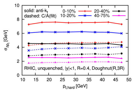
So far, we have only considered central collisions. Since it is known that non-central collisions give rise to elliptic flow [19, 20, 21, 22, 23, 24, 25, 26, 27], one might worry that this leads to an extra source of background fluctuations and/or non-uniformities, potentially spoiling the subtraction picture discussed so far. One can study this on azimuthally averaged jet samples (as we have been doing so far) or as a function of the azimuthal angle, $\Delta\phi$, between the jet and the reaction plane. As above, we use Hydjet v1.6, whose underlying HYDRO component includes a simulation of elliptic flow [107].

We have generated heavy-ion background events for RHIC in four different centrality bins: 0-10% (as above), 10-20%, 20-40% and 40-75%, with $v_{2}$ values respectively of $1.7\%$, $3.3\%$, $5.0\%$ and $5.3\%$.

We first examine azimuthally averaged results, repeating the studies of the previous sections for each of the centrality bins. We find that the results for the average shift, $\left\langle\Delta p_{t}\right\rangle$, are largely independent of centrality, as expected if the elliptic flow effects disappear when averaged over $\phi$. The results for the dispersion are shown in fig. 4.8. We observe that the dispersion decreases with increasing non-centrality. Even though one might expect adverse effects from elliptic flow, the heavy-ion background decreases rapidly when one moves from central to peripheral collisions, and this directly translates into a decrease of $\sigma_{\Delta p_{t}}$.

The first conclusion from this centrality-dependence study is therefore that the subtraction methods presented in this paper appear to be applicable also for azimuthally averaged observables in non-central collisions.

Figure 4.9: $\phi$ dependence of the $\Delta p_{t}$ shift at RHIC, for the $0-10\%$ centrality bin. Left: for three different ranges for the anti-$k_{t}$ algorithm; right: for three different jet algorithms for the doughnut($R,3R$) range. The absolute size of the $\phi$ dependence is similar for centralities up to $40\%$ and then decreases beyond.

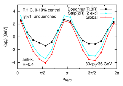
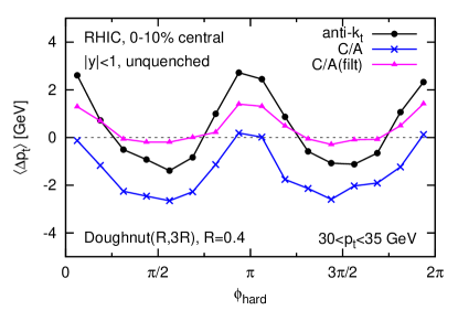
We next consider results as a function of $\Delta\phi$, which is relevant if one wishes to examine the correlation between jet quenching and the reaction plane. An issue in real experimental studies is the determination of the reaction plane, and the extent to which it is affected by the presence of hard jets. In the Hydjet simulations, this problem does not arise because the reaction plane always corresponds to $\phi=0$. Figure 4.9 (left) shows the average $\Delta p_{t}$ as a function of $\Delta\phi$ for the anti-$k_{t}$ algorithm and several different background-estimation ranges, for the $0-10\%$ centrality bin for RHIC. The strip range shows significant $\Delta\phi$ dependence, which is because a determination of $\rho$ averaged over all $\phi$ cannot possibly account for the local $\phi$-dependence induced by the elliptic flow. Other ranges, such as the doughnut range, instead cover a more limited region in $\phi$. They should therefore be able to provide information on the $\phi$-dependence of the background. However, since their extent in $\phi$ tends to be significantly larger than that of the jet, and $\rho$ varies relevantly over that extent, some residual $\phi$ dependence remains in $\left\langle\Delta p_{t}\right\rangle$ after subtraction. The right-hand plot of figure 4.9 shows that the effect is reduced with filtering, as is to be expected since its initial background contamination is smaller. The conclusion from this part of the study is that residual $\phi$-dependent offsets may need to be corrected for explicitly in any studies of jets and their correlations with the reaction plane. The investigation of extensions to our background subtraction procedure to address this issue will be the subject of future work.

4.3.5 Quenching effects

An important issue we wish to investigate is how the phenomenon of jet quenching (i.e. medium effects on parton fragmentation) may affect the picture developed so far. The precise nature of jet quenching beyond its basic analytic properties (see e.g.  [83, 84]) is certainly hard to estimate in detail, especially at the LHC, where experimental data from, say, flow or particle spectra measurements are not yet available for the tuning of the Monte Carlo simulations. Additionally, the implementation of Monte-Carlo generators that incorporate the analytic features of jet quenching models is currently a very active field [92, 108, 109]. We may therefore expect a more robust and complete picture of jet quenching in the near future, related to existing and forthcoming PbPb data at the LHC.

In this section, we examine the robustness of our HI background subtraction in the presence of (simulated) jet quenching. For this purpose we have used two available models which allow one to simulate quenched hard jets, Pyquen, which is used by Hydjet v1.6, and QPythia. Pyquen has been run with the parameters listed in footnote 5 for the LHC, and with $\texttt{T0}=0.5\,\mathrm{GeV}$, $\texttt{tau0}=0.4$ fm and $\texttt{nf}=2$ for RHIC. For QPythia we have tested two options for the values of the transport coefficient and the medium length ($\hat{q}=3$ GeV²/fm, $L=5$ fm and $\hat{q}=1$ GeV²/fm, $L=6$ fm), with similar results. No serious attempt has been made to tune the two codes with each other or with the experimental data, beyond what is already suggested by the code defaults: in the absence of strong experimental constraints on the details of the quenching effects, this allows us to verify the robustness of our results for a range of conditions.

As in sections 4.3.2 and 4.3.3, we have embedded the hard Pyquen or QPythia events in a Hydjet v1.6 background and tested the effectiveness of the background subtraction for different choices of algorithm. We shall restrict our attention to the anti-$k_{t}$ and C/A(filt) algorithms, as they appear to be the optimal choices from our analysis so far.

Figure 4.10: Average $p_{t}$ shift for background-subtracted jets with the anti-$k_{t}$ and C/A(filt) jet algorithms. The dashed lines correspond to unquenched hard jets (Pythia) and the solid ones to quenched hard jets (Pyquen). Results are shown for RHIC kinematics on the left plot and for the LHC on the right one.

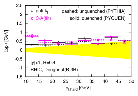
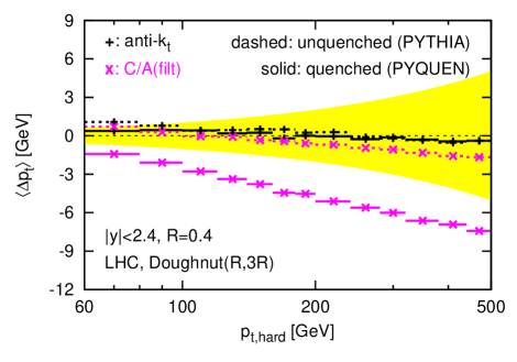
We have found that the jet-matching efficiencies are still high, with essentially no changes at RHIC, and at LHC a doubling of the (small) inefficiencies that we saw in fig. 4.2(right). The dispersions $\sigma_{\Delta p_{t}}$ are also not significantly affected within our sample of jet-quenching simulations. We therefore concentrate on the $\left\langle\Delta p_{t}\right\rangle$ offset, which is plotted in fig. 4.10 for Pyquen. The results are shown for both RHIC and the LHC. In the case of RHIC, and for the whole $p_{t}$ range up to about 50 GeV, quenching can be seen not to significantly affect the subtraction offset $\langle\Delta p_{t}\rangle$ (within the usual uncertainty related to the choice of range, which was shown in fig. 4.3). In the LHC case, instead, while the shift obtained using the anti-$k_{t}$ algorithm is largely similar to the unquenched case, the C/A(filt) algorithm performance can be seen to deteriorate slightly when quenching is turned on, all the more so at very large transverse momentum. The $k_{t}$ and the C/A algorithms are not shown for clarity, but they share the behaviour of C/A(filt). This deterioration of the quality of the subtraction can be traced back to an increased back-reaction compared to the unquenched jets. Anti-$k_{t}$ jets do not suffer from this effect as a consequence of the usual rigidity of this algorithm. In the case of C/A(filt), one should nevertheless emphasise that an error of (at most) 10 GeV on the reconstruction of a 500 GeV jet is still only a 2% effect. This is modest, both relative to the likely experimental precision and to the expected effect of quenching on the overall jet $p_{t}$, predicted by Pyquen to be at the level of $10\%$ at this $p_{t}$.

Though for brevity we have not explicitly shown them, the results with QPythia are very similar.

Before closing this section, we reiterate that we have only investigated simple models for quenching and that our results are meant just to give a first estimate of the effects that one might have to deal with in the case of quenched jets. One will be able to address this question more extensively as more data is collected at the LHC and the dynamics of jet quenching in QCD is better understood, together with the development of better “quenched” Monte Carlo generators.

4.4 Further details and analytic estimates

4.4.1 Back reaction contribution to the dispersion

In the context of heavy-ion collisions, where the residual resolution-degradation effects on the jets can be relatively large, it is interesting to look a bit deeper in the various sources that contribute to the dispersion. The natural candidates are the UE fluctuations themselves and residual uncertainties on the estimation of $\rho$ (which have been made small by choosing a large enough range). Here we discuss two additional sources: the dispersion in the back-reaction which starts kicking in at large $p_{t}$ and the uncertainty in our calculation of the jet area.

Figure 4.11: The decomposition of the dispersion into back-reaction and “background” components (including misestimation of $\rho$). The left-hand plot is for the anti-$k_{t}$ algorithm and the right-hand one for C/A(filt). Both correspond to LHC collisions at $\sqrt{s_{NN}}=5.5\,\mathrm{TeV}$.

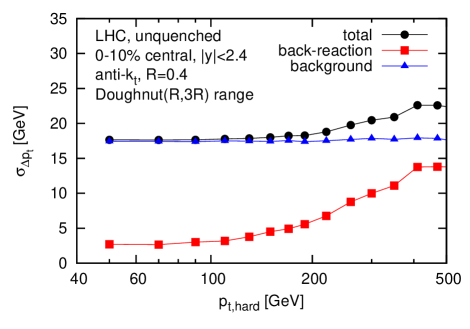
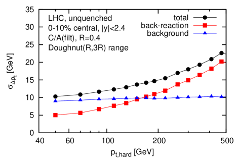
We stated, in section 4.3.3, that the increase of the dispersion at high $p_{t}$ seen in fig. 4.7 was mainly due to back-reaction. This is made explicit in fig. 4.11, which decomposes the dispersion into its two components: that associated with the back-reaction, $\sigma_{\Delta p_{t}}^{\mathrm{BR}}$ and that associated with background fluctuations and misestimation of $\rho$ (defined as $[\sigma_{\Delta p_{t}}^{2}-(\sigma_{\Delta p_{t}}^{\mathrm{BR}})^{2}]^{\frac{1}{2}}$). As already observed in $pp$ collisions (see Section 3.2.4), one sees that the background-fluctuation component is essentially independent of $p_{t}$, while the back-reaction dispersion has a noticeable $p_{t}$ dependence. The flatness of the residual, non-back-reaction, component is again observed and is expected since the anomalous dimension of the jet area is zero for anti-$k_{t}$ and small for C/A (with or without filtering), and in any case leads to a weak scaling with $p_{t}$, as $\ln\ln p_{t}$. Furthermore, there is roughly a factor of $1/\sqrt{2}$ between anti-$k_{t}$ and C/A(filt), as expected based on a proportionality of the dispersion to the square-root of the jet area.

Figure 4.12: Dispersion, $\sigma_{\Delta p_{t}}$, for RHIC, as a function of the jet $p_{t}$, with two different choices for the ghost area, $0.01$ and $0.0025$.

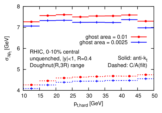
4.4.2 Quality of area determination

One further source of $\Delta p_{t}$ fluctuations can come from imperfect estimation of the area of the jets. We recall that throughout this article we have used soft ghosts, each with area of $0.01$, in order to establish the jet area. That implies a corresponding finite resolution on the jet area and related poor estimation of the exact edges of the jets, which can have an impact on the amount of background that one subtracts from each jet, and, consequently, on the final dispersion. It is therefore interesting to see, figure 4.12, that the dispersion $\sigma_{\Delta p_{t}}$ is reduced by about $0.2-0.4\,\mathrm{GeV}$ if one lowers the ghost area to $0.0025$.

While this does not affect any of the conclusions of our paper, it does suggest that for a full experimental analysis there are benefits to be had from using a ghost area that is smaller than the default FastJet setting of $0.01$. These observations are behind one the points made in our final recommendations, Section 2.8.

4.4.3 Relative importance of average shift and dispersion

To close this section, we examine the relative importance of the average shift and its dispersion, taking the illustrative example of their impact on the inclusive jet cross-section as a function of $p_{t}$. This follows our simple description introduced in Section 2.2 where we have seen that the true $p_{t}$ spectrum decays exponentially i.e.

$$\frac{d\sigma^{pp}}{dp_{t}}=\frac{\sigma_{0}}{\kappa}\,e^{-p_{t}/\kappa}.$$ (4.4)

The reconstructed spectrum, after embedding in a heavy-ion background and applying subtraction will be multiplied by a factor

$$\exp\left(\frac{\left\langle\Delta p_{t}\right\rangle}{\kappa}+\frac{\sigma_{\Delta p_{t}}^{2}}{2\kappa^{2}}\right),$$ (4.5)

as obtained in Eq. (2.8). For a given reconstructed $p_{t}$, the most likely original true transverse momentum is given by Eq. (2.10) and reads

$$\text{most likely}\;p_{t}^{pp}\simeq p_{t}^{AA,{\rm sub}}-\left\langle\Delta p_{t}\right\rangle-\frac{\sigma_{\Delta p_{t}}^{2}}{\kappa}\,,$$ (4.6)

where we have neglected the small impact of subtraction on the $pp$ jets.

To illustrate these effects quantitatively, let us first take the example of RHIC, where between 10 and 60 GeV, the cross-section is well approximated by Eq. (4.4) with $\kappa=3.3$ GeV. Both the anti-$k_{t}$ and C/A(filt) have $\left\langle\Delta p_{t}\right\rangle\simeq 0$, leaving only the dispersion effect. In the case of the anti-$k_{t}$ (respectively C/A(filt)) algorithm, we see from fig. 4.7 that $\sigma_{\Delta p_{t}}\simeq 7.5\,\mathrm{GeV}$ ($4.8\,\mathrm{GeV}$), which gives a multiplicative factor of about 12 (3). For a given reconstructed $p_{t}$, the most likely true $p_{t}$ is about $17\,\mathrm{GeV}$ ($7\,\mathrm{GeV}$) smaller. In comparison, for C/A ($k_{t}$), with $\left\langle\Delta p_{t}\right\rangle\simeq-1.5\,\mathrm{GeV}$ ($-3.5\,\mathrm{GeV}$) (fig. 4.5) and $\sigma_{\Delta p_{t}}\simeq 6.5\,\mathrm{GeV}$ (similar for $k_{t}$) there is a partial compensation between factors of $0.64$ ($0.35$) and $6.7$ coming respectively from the shift and dispersion, yielding an overall factor of about $4$ ($2.3$), while the most likely true $p_{t}$ is about $14\,\mathrm{GeV}$ ($12\,\mathrm{GeV}$) smaller than the reconstructed $p_{t}$.

At the LHC ($\sqrt{s_{NN}}=5.5\,\mathrm{TeV}$), Eq. (4.4) is a less accurate approximation. Nevertheless, for $p_{t}\sim 100-150\,\mathrm{GeV}$, it is not too unreasonable to take $\kappa=20\,\mathrm{GeV}$ and examine the consequences. For anti-$k_{t}$ (respectively C/A(filt)), we have $\left\langle\Delta p_{t}\right\rangle\simeq 0$ (also for C/A(filt)) and $\sigma_{\Delta p_{t}}\simeq 18\,\mathrm{GeV}$ ($13\,\mathrm{GeV}$), giving a multiplicative factor of $1.5$ ($1.2$), i.e. far smaller corrections than at RHIC. For a given reconstructed $p_{t}$, the most likely true $p_{t}$ is about $16\,\mathrm{GeV}$ ($8\,\mathrm{GeV}$) smaller, rather similar to the values we found at RHIC (though smaller in relative terms, since the $p_{t}$’s are higher), with the increase in $\sigma$ being compensated by the increase in $\kappa$.

In the LHC case, it is also worth commenting on the results for the $k_{t}$ algorithm, since this is what was used in the original work from Ref. [5]: we have $\left\langle\Delta p_{t}\right\rangle\simeq-8\,\mathrm{GeV}$ and $\sigma_{\Delta p_{t}}\simeq 18\,\mathrm{GeV}$, giving a multiplicative factor of $1.05$, which is consistent with the near perfect agreement that was seen there between the $pp$ and subtracted $AA$ spectra. That agreement does not however imply perfect reconstruction, since the most likely $p_{t}^{pp}$ is about $7\,\mathrm{GeV}$ lower than $p_{t}^{AA,{\rm sub}}$.

Though the above numbers give an idea of the relative difficulties of using different algorithms at RHIC and LHC, experimentally what matters most will be the systematic errors on the correction factors (for example due to poorly understood non-Gaussian tails of the $\Delta p_{t}$ distribution). Note also that a compensation between shift and dispersion factors, as happens for example with the C/A algorithm, is unlikely to reduce the overall systematic errors.

4.4.4 Fluctuations in extracted $\rho$

In section 4.2.2, we gave an estimate of the minimum size of a range one should require for determining $\rho$, given a requirement that fluctuations in the determination of $\rho$ should be moderate. We give the details of the computation in this Section.

We start from the fact that the error made on the estimation of the background density $\rho$ will translate into an increase of the dispersion $\sigma_{\Delta p_{t}}$: on one hand, the dominant contribution to $\sigma_{\Delta p_{t}}$ comes from the intra-event fluctuations of the background i.e. is of order $\sigma\sqrt{A_{\rm jet}}$ with $A_{\rm jet}$ the jet area; on the other hand, the dispersion $S_{\Delta\rho}$ of the misestimation of $\rho$ leads to an additional dispersion on the reconstructed jet $p_{t}$ of $S_{\Delta\rho}A_{\rm jet}$. As we will show in the next Chapter, $S_{\Delta\rho}$ can be estimated analytically, see Eq. (5.103). Adding these two sources of dispersion in quadrature and using (5.103), with $A_{\rm tot}=A_{\cal R}$ the area of the range under consideration, we get

$$\sigma_{\Delta p_{t}}\simeq\sigma\left(A_{\rm jet}+\frac{\pi A_{\rm jet}^{2}}{2A_{\cal R}}\right)^{\frac{1}{2}}.$$ (4.7)

If we ask e.g. that the contribution to the total dispersion coming from the misestimation of the background be no more than a fraction $\epsilon$ of the total $\sigma_{\Delta p_{t}}$, then we obtain the requirement

$$A_{\cal R}\gtrsim A_{\min}\simeq\frac{\pi}{4}\frac{A_{\rm jet}}{\epsilon}\,.$$ (4.8)

For anti-$k_{t}$ jets of radius $R$, with $A_{\rm jet}\simeq\pi R^{2}$, this translates to

$$A_{\cal R}\gtrsim\frac{\pi^{2}}{4}\frac{R^{2}}{\epsilon}\simeq 25R^{2}\,,$$ (4.9)

where the numerical result has been given for $\epsilon=0.1$. For $R=0.4$, it becomes $A_{\cal R}\gtrsim 4$.

We can also cast this result in terms of the number of jets that must be present in ${\cal R}$. Assuming that the jets used to estimate $\rho$ have a mean area of $0.55\pi R_{\rho}^{2}$, we find a minimal number of jets ,

$$n_{\min}\simeq\frac{A_{\min}}{0.55\pi R_{\rho}^{2}}\simeq\frac{1.4}{\epsilon}\frac{R^{2}}{R_{\rho}^{2}}\,,$$ (4.10)

where, as before, we have taken $A_{\mathrm{jet}}\simeq\pi R^{2}$. Taking the numbers quoted above and $R_{\rho}=0.5$, as used in the main body of the article, this gives $n_{\min}\simeq 9$.

4.4.5 Hard-jet bias in extracted $\rho$

As we will show in our detailed analytic studies, see Section 5.2.3, the presence of hard jets and initial-state radiation leads to a bias in the extraction of $\rho$ of

$$\left\langle\Delta\rho\right\rangle\simeq\sigma R_{\rho}\sqrt{\frac{\pi c_{J}}{2}}\frac{\left\langle n_{h}\right\rangle}{A_{\cal R}}\,$$ (4.11)

where $c_{J}\simeq 2$ is a numerical constant and $\left\langle n_{h}\right\rangle$ is the average number of “hard” jets (those above the scale of the background fluctuations, including initial-state radiation); $\left\langle n_{h}\right\rangle$ is given by

$$\frac{\left\langle n_{h}\right\rangle}{A_{\cal R}}\simeq\frac{n_{b}}{A_{\cal R}}+\frac{C_{i}}{\pi^{2}}\frac{L}{b_{0}}\,,\qquad\quad L=\ln\frac{\alpha_{s}\left(\sqrt{c_{J}}\sigma R_{\rho}\right)}{\alpha_{s}(p_{t})}\,,$$ (4.12)

where $n_{b}$ is the number of “Born” partons from the underlying $2\to 2$ scattering that enter the region $\cal R$, while $b_{0}=(11C_{A}-2n_{f})/(12\pi)$ is the first coefficient of the QCD $\beta$-function. Contrarily to the original case of UE studies in $pp$ collisions [37], in the case of a large background like the UE in $AA$ collisions, one can safely ignore the impact of the second term in (4.12). We thus arrive at the result

$$\left\langle\Delta\rho\right\rangle\simeq\sigma R_{\rho}\sqrt{\frac{\pi c_{J}}{2}}\frac{n_{b}}{A_{\cal R}}\simeq 1.8\,\sigma R_{\rho}\frac{n_{b}}{A_{\cal R}}\,.$$ (4.13)

Note that the presence of hard jets and initial-state radiation also affects the fluctuations in the misestimation of $\rho$ and this should in principle have been included in the estimates of Section 4.4.4. However, while the effect is not completely negligible, to within the accuracy that is relevant for us (a few tens of percent in the estimation of a minimal $A_{\cal R}$) it does not significantly alter the picture outlined there.

4.4.6 Subtraction bias due to filtering

We have seen from fig. 4.5 in section 4.3.3 that the subtraction differs when we use the C/A algorithm with and without filtering. Since this difference is not due to back-reaction (see fig. 4.6), it has to be due to the subtraction itself.

The difference comes from a bias introduced by the selection of the two hardest subjets during filtering. The dominant contribution comes when only one subjet, that we shall assume harder than all the others, contains the hard radiation, all the other subjets being pure background. In that case, the selection of the hardest of these pure-background subjets as the second subjet to be kept tends to pick positive fluctuations of the background. This in turn results in a positive offset compared to pure C/A clustering, as observed in section 4.3.3.

To compute the effect analytically, let us thus assume that we have one hard subjet and $n_{\rm bkg}$ pure-background subjets of area ${\cal A}_{g}=0.55\pi R_{\rm filt}^{2}$ (see Section. 5.1.2). After subtraction, the momentum of each of the pure-background subjet can be approximated as having a Gaussian distribution of average zero and dispersion $\sigma\sqrt{{\cal A}_{g}}$. Assuming that the “hard” subjet’s transverse momentum remains larger than that of all the background jets, the 2 subjets that will be kept by the filter are the hard subjet (subtracted) and the hardest of all the subtracted background jets. The momentum distribution of the latter is given by the maximum of the $n_{\rm bkg}$ Gaussian distributions. We are only interested here in computing the average bias introduced by the filtering procedure, which is then given by

$$\left\langle(\Delta p_{t})_{\rm filt}\right\rangle\simeq\int\prod_{k=1}^{n_{\rm bkg}}\left(dp_{t,k}\,\frac{1}{\sqrt{2\pi{\cal A}_{g}}\sigma}e^{-\frac{p_{t,k}^{2}}{2{\cal A}_{g}\sigma^{2}}}\right)\>{\rm max}\left(p_{t,1},\dots,p_{t,n_{\rm bkg}}\right)$$

For the typical case $R_{\rm filt}=R/2$ and $n_{\rm bkg}=3$, one finds

$$\left\langle(\Delta p_{t})_{\rm filt}\right\rangle\simeq\frac{3\sqrt{{\cal A}_{g}}\sigma}{2\sqrt{\pi}}\simeq 0.56\,R\sigma.$$ (4.14)

If we insert in that expression the typical values for the fluctuations quoted in section 4.3 and $R=0.4$, we find average biases of 2 GeV for RHIC and 4.5 GeV at the LHC, which are in good agreement with the differences observed between C/A with and without filtering in fig. 4.5.

4.5 The issue of fakes

While the goal of this paper is not to discuss the issue of “fake-jets” in detail, it is a question that has been the subject of substantial debate recently (see for example [95, 110]). Here, therefore, we wish to devote a few words to it and discuss how it relates to our background-subtraction results so far.

In a picture in which the soft background and the hard jets are independent of each other, one way of thinking about a fake jet is that it is a reconstructed jet (with significant $p_{t}$) that is due not to the presence of an actual hard jet, but rather due to an upwards fluctuation of the soft background. The difficulty with this definition is that there is no uniquely-defined separation between “hard” jets and soft background. This can be illustrated with the example of how Hydjet simulates RHIC collisions: one event typically consists of a soft HYDRO background supplemented with $\sim 60$ $pp$ collisions, each simulated with a minimum $p_{t}$ cut of $2.6\,\mathrm{GeV}$ on the $2\to 2$ scattering. To some approximation, the properties of the full heavy-ion events remain relatively unchanged if one modifies the number of $pp$ collisions and corresponding $p_{t}$ cut and also retunes the soft background. The fact that this changes the number of hard jets provides one illustration of the issue that the soft/hard separation is ill-defined. Additionally, while there are $\sim 60$ semi-hard $pp$ collisions ($\sim 120$ mostly central semi-hard jets) in an event, there is only space within (say) the acceptance of RHIC for ${\cal O}\left(40\right)$ jets. Thus there is essentially no region in an event which does not have a semi-hard jet. From this point of view, every reconstructed jet corresponds to a (semi-)hard $pp$ jet and there are no fake jets at all.

4.5.1 Inclusive analyses

For inclusive analyses, such as a measurement of the inclusive jet spectrum, this last point is particularly relevant, because every jet in the event contributes to the measurement. Then, the issue of fakes can be viewed as one of unfolding. In that respect it becomes instructive, for a given bin of the reconstructed heavy-ion $p_{t}$, to ask what the corresponding matched $pp$ jet transverse momenta were. Specifically, we define a quantity $O(p_{t}^{AA,{\rm sub}},p_{t}^{pp})$, the distribution of the $pp$ “origin”, $p_{t}^{pp}$, of a heavy-ion jet with subtracted transverse momentum $p_{t}^{AA,{\rm sub}}$. If the origin $O(p_{t}^{AA,{\rm sub}},p_{t}^{pp})$ is dominated by a region of $p_{t}^{pp}$ of the same order as $p_{t}^{AA,{\rm sub}}$, then that tells us that the jets being reconstructed are truly hard. If, on the other hand, it is dominated by $p_{t}^{pp}$ near zero, then that is a sign that apparently hard heavy-ion jets are mostly due to upwards fluctuations of the background superimposed on low-$p_{t}$ $pp$ jets, making the unfolding more delicate.

Figure 4.13: The $p_{t}$ distribution of the $pp$ jet corresponding to a given bin of reconstructed heavy-ion jet $p_{t}^{AA,{\rm sub}}$ at RHIC, i.e. $O(p_{t}^{AA,{\rm sub}},p_{t}^{pp})$ as a function of $p_{t}^{pp}$ for a given bin of $p_{t}^{AA,{\rm sub}}$. The upper row is for the anti-$k_{t}$ algorithm, while the lower row is for C/A(filt). Each column corresponds to a different $p_{t}^{AA,{\rm sub}}$ bin, as indicated by the vertical band in each plot. Cases in which the histogram is broad or peaked near $0$ are indicative of the need for special care in the unfolding procedure. These plots were generated using approximately 90 million events. Each plot has been normalised to the number of events in the corresponding $p_{t}^{AA,{\rm sub}}$ bin.

Figure 4.14: Same as fig. 4.13 for LHC kinematics (PbPb, $\sqrt{s}=5.5\,\mathrm{TeV}$), generated with approximately 16 million events. Note the use of a smaller rapidity range here, $|y|<1$, compared to the earlier LHC plots.

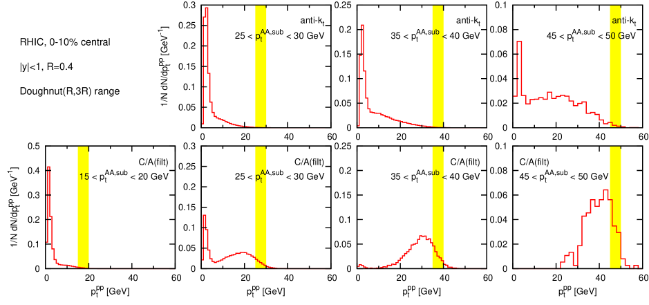
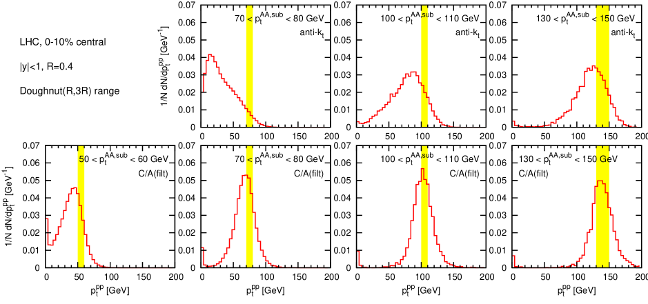
In figure 4.13 we show the origins of heavy-ion jets as determined in our Hydjet simulations. The upper row provides the origin plots for anti-$k_{t}$ jets at RHIC. Each plot corresponds to one bin of $p_{t}^{AA,{\rm sub}}$, and shows $O(p_{t}^{AA,{\rm sub}},p_{t}^{pp})$ as a function of $p_{t}^{pp}$. At moderate $p_{t}^{AA,{\rm sub}}$, the $25-30\,\mathrm{GeV}$ bin, the origin is dominated by low $p_{t}^{pp}$. This is perhaps not surprising, given the result in subsection 4.4.3 that the $p_{t}^{pp}$ origin is expected to be $\sim 17\,\mathrm{GeV}$ lower than $p_{t}^{AA,{\rm sub}}$ for anti-$k_{t}$ jets — additionally, that result assumed an exponential spectrum for the inclusive jet distribution, whereas the distribution rises substantially faster towards low $p_{t}^{pp}$. As $p_{t}^{AA,{\rm sub}}$ increases one sees that the contribution of high $p_{t}^{pp}$ jets increases, in a manner not too inconsistent with the expected $\sim 17\,\mathrm{GeV}$ shift, though the $p_{t}^{pp}$ distribution remains rather broad and a peak persists at small $p_{t}^{pp}$. These plots suggest that an inclusive jet distribution measurement with the anti-$k_{t}$ algorithm at RHIC is not completely trivial since, up to rather large $p_{t}^{AA,{\rm sub}}$, one is still sensitive to the jet distribution at small values of $p_{t}^{pp}$ where the separation between “hard” jets and the soft medium is less clear. Nevertheless, two points should be kept in mind: firstly, the upper row of fig. 4.13 shows that different $p_{t}^{AA,{\rm sub}}$ have complementary sensitivities to different parts of the $p_{t}^{pp}$ spectrum. Thus it should still be possible to “unfold” the $p_{t}^{AA,{\rm sub}}$ distribution to obtain information about the $p_{t}^{pp}$, unfolding being in any case a standard part of the experimental correction procedure. Secondly STAR quotes [96, 97] a $10\%$ smaller value for $\sigma_{\Delta p_{t}}$ than the $7.5\,\mathrm{GeV}$ that we find in Hydjet. Such a reduction can make it noticeably easier to perform the unfolding.

The impact of a reduction in $\sigma_{\Delta p_{t}}$ is illustrated in the lower row of fig. 4.13, which shows the result for C/A(filt). Here, even the $25-30\,\mathrm{GeV}$ bin for $p_{t}^{AA,{\rm sub}}$ shows a moderate-$p_{t}$ peak in the distribution of $p_{t}^{pp}$, and in the $35-40\,\mathrm{GeV}$ bin the low-$p_{t}$ “fake” peak has disappeared almost entirely. Furthermore, the $p_{t}^{pp}$ peak is centred about $7\,\mathrm{GeV}$ lower than the centre of the $p_{t}^{AA,{\rm sub}}$ bin, remarkably consistent with the calculations of section 4.4.3. Overall, therefore, unfolding with C/A(filt) will be easier than with anti-$k_{t}$.

Corresponding plots for the LHC are shown in fig. 4.14. While C/A(filt)’s lower dispersion still gives it an advantage over anti-$k_{t}$, for $\smash{p_{t}^{AA,{\rm sub}}}\gtrsim 80\,\mathrm{GeV}$, anti-$k_{t}$ does now reach a domain where the original $pp$ jets are themselves always hard.

Procedures to reject fake jets have been proposed, in [111, 112]. They are based on a cut on (collinear unsafe) jet shape properties and it is thus unclear how they will be affected by quenching and in particular whether the expected benefit of cutting the low-$p_{t}^{pp}$ peak in Figs. 4.13 and 4.14 outweighs the disadvantage of potentially introducing extra sources of systematic uncertainty at moderate $p_{t}$.

One final comment is that experimental unfolding should provide enough information to produce origin plots like those shown here. As part of the broader discussion about fakes it would probably be instructive for such plots to be shown together with the inclusive-jet results.

4.5.2 Exclusive analyses

An example of an exclusive analysis might be a dijet study, in which one selects the two hardest jets in the event, with transverse momenta $p_{t1}$ and $p_{t2}$, and plots the distribution of $\frac{1}{2}H_{T,2}\equiv\frac{1}{2}(p_{t1}+p_{t2})$. Here one can define “fakes” as corresponding to cases where one or other of the jets fails to match to one of the two hardest among all the jets from the individual $pp$ events. This definition is insensitive to the soft/hard boundary in a simulation such as Hydjet, because it naturally picks out hard $pp$ jets that are far above that boundary. And, by concentrating on just two jets, it also evades the problem of high occupancy from the large multiplicity of semi-hard $pp$ collisions. This simplification of the definition of fakes is common to many exclusive analyses, because they tend to share the feature of identifying just one or two hard reference jets.

The specific case of the exclusive dijet analysis has the added advantage that it is amenable to a data-driven estimation of fakes. One divides the events into two groups, those for which the two hardest jets are on the same side (in azimuth) of the event and those in which they are on opposite sides (a related analysis was presented by STAR in ref. [113]). For events in which one of the two jets is “fake,” the two jets are just as likely to be on the same side as on the opposite side. This is not the case for non-fake jets, given that the two hardest “true” jets nearly always come from the same $pp$ event and so have to be on opposite sides. Thus by counting the number of same-side versus opposite-side dijets in a given $\frac{1}{2}H_{T,2}$ bin, one immediately has an estimate of the fake rate.

Figure 4.15: The distribution of $\frac{1}{2}H_{T,2}$ obtained from the two hardest full, subtracted heavy-ion jets in each event at RHIC, as obtained from simulations with Hydjet 1.6. The left-hand plot is for anti-$k_{t}$ and the right-hand plot for C/A(filt). The same-side curves give an approximate measure of (half of) the contribution of “fake” jets to the dijet spectrum.

Figure 4.16: Same as fig. 4.16 for LHC kinematics.

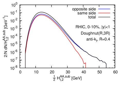
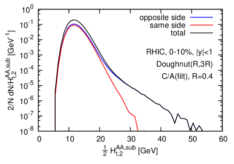
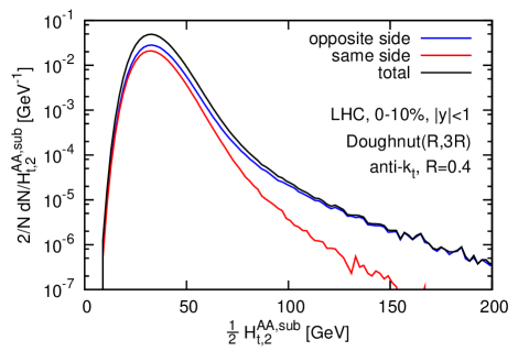
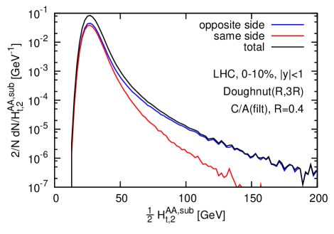
This is illustrated in fig. 4.16, which shows the distribution at RHIC of the full, subtracted $\frac{1}{2}H_{T,2}$ result, together with its separation into opposite-side and same-side components. One sees that in the peak region, the opposite and same-side distributions are very similar, indicating a predominantly “fake” origin for at least one of two hardest jets (they are not quite identical, because there is less phase-space on the same side for a second jet than there is on the away side). However above a certain full, reconstructed $\frac{1}{2}H_{T,2}$ value, about $30\,\mathrm{GeV}$ for anti-$k_{t}$ and $20\,\mathrm{GeV}$ for C/A(filt) the same-side distribution starts to fall far more rapidly than the opposite-side one, indicating that the measurement is now dominated by “true” pairs of jets.

The LHC results, fig. 4.16, are qualitatively similar, with the same-side spectrum starting to fall off more steeply than the opposite-side one around $70\,\mathrm{GeV}$ for the anti-$k_{t}$ algorithm and $50\,\mathrm{GeV}$ for C/A(filt).

One can also examine origin plots for $H_{T,2}$, in analogy with the Monte Carlo analysis of section 4.5.1. For brevity, we refrain from showing them here, and restrict ourselves to the comment that in the region of $H_{T,2}$ where the result is dominated by opposite-side pairs, the origin plots are consistent with a purely hard origin for the dijets.

4.6 Summary and discussions

We have shown that the area–median subtraction method gives good performance to subtract the large heavy-ion UE. We have tested different choices of range to estimate the rapidity dependence and observed little difference between various ranges, as long as they are chosen to be localised in the vicinity of the jet of interest and of sufficient size (at least 4 units of area for jets with $R=0.4$).

As for the quality measures, the offset can be brought close to zero by using the anti-$k_{t}$ algorithm, while the $k_{t}$ algorithm has the largest offset; the Cambridge/Aachen (C/A) algorithm with filtering also gives a small offset, however this seems to have been due to a fortuitous cancellation between two only partially related effects. The dispersion is comparable for anti-$k_{t}$, C/A and $k_{t}$, but significantly smaller for C/A(filt) (except at high transverse momenta for LHC), as a consequence of its smaller jet area. Among the different algorithms, anti-$k_{t}$ is the most robust with respect to quenching effects, and C/A(filt) seems reasonably robust at RHIC, though a little less so at the LHC. The precise numerical results for offset and dispersion can depend a little on the details of the simulation and the analysis, however the general pattern remains.

Overall our results indicate that the area-based subtraction method seems well suited for jet reconstruction in heavy-ion collisions. Two jet-algorithm choices were found to perform particularly well: anti-$k_{t}$, which has small offsets but larger fluctuations, and C/A with filtering, for which the offsets may be harder to control, but for which the fluctuations are significantly reduced, with consequent advantages for the unfolding of experimentally measured jet spectra. Ultimately, we suspect that carrying out parallel analyses with these two choices may help maximise the reliability of jet results in HI collisions.

4.7 Jet fragmentation function

The last extension of the area–median approach we want to validate is its application to the subtraction of pileup contamination to the fragmentation function (moments), as described in Section 2.7.4. We shall apply it here to heavy-ion collisions, where it is considered as one of the first observables that one would measure to study jet-quenching effects [114, 115, 93, 116, 117, 118, 119].

Details of the simulation.

Before proceeding with the results, it is useful to detail the terminology and simulation tools that we have used.

What we call ‘hard’ jets in QCD are simulated in proton-proton ($pp$) collisions using Pythia 6.425 in dijet mode with the DW tune [120]. We have not included any $pp$ underlying event (UE), its effect being minimal in this context anyway. Jets including quenching effects have been generated using Pyquen, v1.5.1, as included in Hydjet [107, 82]. We consider all hadrons, not just charged tracks, and take $\pi_{0}$’s to be stable, so that we are still considering genuine hadron distributions.

The heavy-ion background (also called underlying event) is simulated using Hydjet v1.6 for 0-10% centrality and, where needed, it is superimposed to the hard event generated by Pythia. This has been found [80] to be in good agreement with the experimental measurements of background fluctuations by ALICE [121]. The jets observed in this combined event will be denoted as ‘full’ jets.

All events are generated for either $pp$ or lead–lead (PbPb) collisions at the LHC, with a centre-of-mass energy of 2.76 TeV per nucleon-nucleon collision. Jets are reconstructed using the anti-$k_{t}$ algorithm with $R=0.4$, as implemented in FastJet. In estimating the jet’s $p_{t}$, the HI background is subtracted using the area–median method using $k_{t}$ jets with $R=0.4$ to estimate $\rho$. At most the two hardest jets passing a hard cut on the subtracted transverse momentum (see below) are subsequently used for the fragmentation function analysis. The cuts that we shall use are $100\,\mathrm{GeV}$ and $200\,\mathrm{GeV}$.

Effect of the background.

The addition of the heavy-ion background has the potential to modify a measured fragmentation function in two ways. Firstly, the jet’s $p_{t}$ is modified, affecting the normalisation of $z$ in Eq. (2.41). Secondly, the heavy-ion background adds many extra particles to the jet, predominantly at low momenta.

To appreciate the impact of the extra particles in the jet from the heavy-ion background, it is instructive to first examine the “Pythia+Hydjet” dashed red curves of Fig. 4.17. These show the FF extracted in heavy-ion collisions, without any subtraction of the background contribution to the FF, but always using a $z$ value defined such that the jet’s $p_{t}$ has been corrected for the expected HI background contamination (as is standard in the experimental measurements). At this stage we will not perform any unfolding to account for fluctuations in the HI background.

One sees how the FF acquires a ‘bump’ in the soft region, which lies at larger $\xi$ (smaller $z$) than the maximum in the original $pp$ result (blue solid line) and is up to two orders of magnitude higher. For the moments, this presence of the background is seen as a steep increase in the small-$N$ region, taking the curve far off the scale.

At large $z$ (small $\xi$), the impact of the addition of the background is only barely visible, as might be expected given that it is dominated by soft particles. However, this visually small effect is partially an artefact of the logarithmic scale used to show the FF versus $z$. Considering instead the moments, one sees that there is a non-negligible reduction in the FF at large $N$. This is perhaps surprising given that the background adds particles. It is a feature related to the interplay between background fluctuations and the steeply falling jet spectrum. It is well known by the experiments and is related to the effects discussed at the end of Section. 2.6.

Figure 4.17: Jet fragmentation functions shown for plain Pythia, with the addition of the heavy-ion background (Pythia+Hydjet) and after subtraction of the heavy-ion background ($z$-subtracted and $N$-subtracted). For the results including the heavy-ion background, the jet $p_{t}$ used to define $z$ is always that after subtraction of the heavy-ion background. As in Fig. B.1, we show the results as a function of $z$ (left), $\xi$ (middle) and for the moments versus $N$ (right). The upper (lower) row has a jet $p_{t}$ threshold of $100\,\mathrm{GeV}$ ($200\,\mathrm{GeV}$).

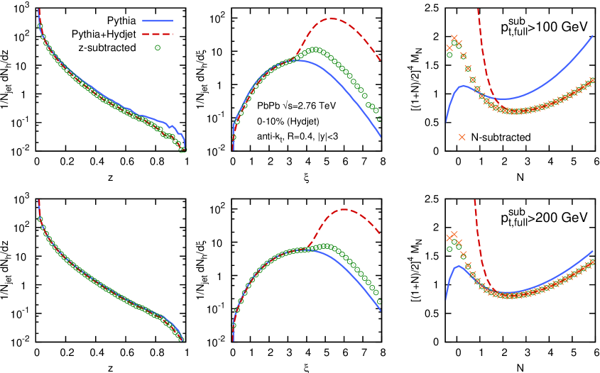
$z$-space subtraction.

The traditional approach to background subtraction from a jet FF involves the construction of a distribution (in $z$ or $\xi$ space) intended to approximate that of background-only particles, and the subtraction of this distribution from the measured one. The way the background-only distribution is determined can vary, the simplest one probably being to consider a region of the event that is expected to be little affected by the hard jets, and measure it there.

To illustrate $z$-space subtraction here, we measure the distribution of hadrons in two regions transverse in azimuth with respect to the axis defined by the dijet event. Event by event, and jet by jet, we subtract those distributions (measured in a patch of phase space with an area equal to that of the jet that one is considering) from the jet fragmentation function. While exact experimental procedures differ in the details, most choices lead to similar results here. Perhaps the main distinction of the experimental procedures is that they sometimes address issues related to flow, which for simplicity we neglect here in our $z$-space subtraction.

The results of applying a $z$-space subtraction are shown in figure 4.17 as green open circles, labelled ‘$z$-subtracted’ (the moments of these $z$-subtracted results are also shown). One sees how these curves come closer to the $pp$ results at small $z$ and small $N$ than do the unsubtracted (dashed red) ones. The agreement improves as the jet $p_{t}$ threshold is increased. However, even with jets of $p_{t}\gtrsim 200$ GeV, this procedure still falls short of an accurate reconstruction of the hard FF. In fact, the region in $z$ where the subtracted FF works well barely extends beyond that selected by simply truncating the unsubtracted FF at low $p_{t,\text{h}}$ so as to avoid the region dominated by the background.

Figure 4.18: The quantities $\rho_{N}$, $\sigma_{N}$ and the correlation coefficient $r_{N}$, shown as a function of $N$ for $0-10\%$ central PbPb collisions $\sqrt{s_{NN}}=2.76\,\mathrm{TeV}$ as obtained from simulations with Hydjet.

Figure 4.19: Jet fragmentation function moments, showing the plain Pythia result, the result after embedding in Hydjet and applying plain subtraction moment-space subtraction (“N-subtracted”) and after the additional improvement to account for correlations (“+ correl”), Eq. (2.55). A quenched result (“Pyquen”) is also shown, to help give an indication of the order of magnitude of quenching effects as compared to residual misreconstruction effects.

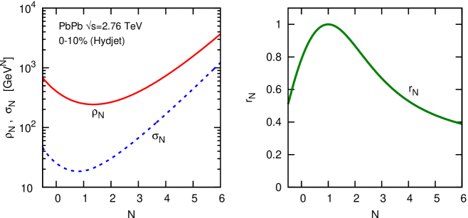
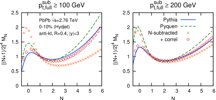
Area–median moments subtraction.

The results for $M_{N}^{\text{sub}}$ are shown in figure 4.17 in the right-most plots, orange crosses labelled ‘$N$-subtracted’. One can see that they are neither better nor worse than the corresponding $z$-subtracted ones, which have been translated to $N$-space and drawn in the same plots for direct comparison (green circles).

In order to provide a fragmentation function reconstruction that is better than that given by the standard $z$-space method, we introduce in the next section an improved background subtraction method that is most straightforwardly applied in moment space.

Area–median improved moments subtraction.

The correction (2.55) can be applied jet by jet to correct for the effects of fluctuations. It requires the prior knowledge of the slope $\kappa$ of the jet cross-section, which can be obtained from $pp$ data, or from simulations. All the other ingredients that enter this equation ($\sigma$, $A$, $S_{N}$, $\sigma_{N}$, $r_{N}$) can instead be determined event-by event or jet-by-jet. In practice we determine $\sigma$, $\sigma_{N}$ and $r_{N}$ from the ensemble of jets contained in an annulus (or “doughnut”) of outer radius $3R$ and inner radius $R$, centred on the jet of interest. Typical values of $\rho_{N}$, $\sigma_{N}$ and $r_{N}$ are presented as a function of $N$ in Fig. 4.18.

We show in figure 4.19 the result of applying Eq. (2.55) to our subtraction in moment space, for two jet $p_{t}$ thresholds. The solid blue curve ($pp$ reference) and orange crosses (N-subtracted) are identical to the results in the rightmost plots in figure 4.17. In addition, figure 4.19 also displays results obtained using Eq. (2.55), shown as red diamonds. One sees how the quality of the agreement with the ‘hard’ blue curve is markedly improved. At low $N$ it is the last, additive, term in Eq. (2.55) that dominates this improvement, accounting for the correlation between a jet’s reconstructed $p_{t}$ fluctuations and the fluctuations in the background’s contribution to the moment; at high $N$ it is the multiplicative $N\sigma^{2}A/S_{1}\kappa$ term that dominates, correcting for the fact that the more common upwards fluctuations in the jet’s reconstructed $p_{t}$ cause the fragmentation $z$ value to be underestimated.

Figure 4.19 also shows (green dashed curve) the jet fragmentation function predicted by the quenching model used in Pyquen. One observes that the remaining deficiencies of the reconstruction are significantly smaller than the difference between the unquenched (solid blue) and the quenched (dashed green) FFs, pointing to a potential discriminating power. This is to be contrasted with subtraction without improvement (orange crosses), which especially in the soft region, $N<1$, fails to describe the blue curve sufficiently well to tell whether quenching (as modelled in Pyquen) is present or simply if an imperfect reconstruction is taking place. This serves as an illustration that the improved subtraction may now be sufficiently good to allow one to discriminate a quenched FF from an unquenched one.

An implementation of the tools needed for the jet fragmentation function subtraction in moments space, as well as for the fluctuations unfolding improvement, is available in fjcontrib.

Chapter 5 Analytic insight

In this chapter we shall review a series of analytic properties related to the area–median pileup subtraction method. These are meant to serve two main purposes: first, jets being QCD objects, there is a clear interest to see if their properties are under analytic control in terms of perturbative QCD; second, we will see that simple analytic estimates allow to grasp a large fraction of the features observed in Monte Carlo simulations.

As far as we are willing to understand QCD aspects of jets and their properties, a large part of this chapter can be seen as a turf for theoretical QCD aficionados with little phenomenological consequences. Nevertheless, the results we obtain often allow for a deeper understanding of the dynamics of jets and can be beneficial in various respects. In the following pages, we shall thus give an extended discussion of the two cornerstones of the area–median method by discussing the analytic properties of jet areas (Section 5.1) and an analytic understanding of the estimation of the pileup energy density $\rho$ (see Section 5.2).

On the second front, there is a long list of cases where simple analytic understanding can help understanding the underlying physics and build a coherent picture of pileup mitigation, as we have already seen a few times in the previous chapters. These often rely on a Gaussian approximation for the pileup $p_{t}$ distribution, simplified distributions for the underlying hard processes and basic understanding of jet areas. We shall provide strong bases for these arguments throughout this chapter.

Finally, as we shall see for example in Section 5.1.6, our analytic investigations open a series of doors towards future developments.

5.1 Properties of jet areas

In the context of pileup subtraction, we are mostly interested in the active jet area. However, passive areas are much simpler to handle since they do not involve the clustering of ghosts — it is tempting, here, to draw an analogy with QED v. QCD where, perturbatively, the latter is very often simpler to manage than the latter because photons do not interact while gluons do. We shall therefore begin with a study of the properties of passive areas.

That said, our goal is to understand the properties of jet areas in perturbative QCD (pQCD). To do that, we start by considering jets made of a single particle, carry on with cases with 2 particles and try, when possible, to extrapolate to multi-particle configurations.

Before going into detailed calculations, we should mention that jet areas are infrared-unsafe quantities, as we will see explicitly in the calculations below. This should not come as a surprise since they are directly constructed from infinitely soft particles (ghosts). In practice, it means that jet areas are sensitive to IR details such as hadronisation. The main goal of this Section is to show that it is nevertheless possible to deduce interesting pieces of information about jet areas from perturbative QCD. Furthermore, since the jet areas are meant to capture the sensitivity of jets to soft radiation (and pileup in particular), we believe that any sensible (i.e. related to the jet’s sensitivity to UE/pileup type contamination) definition of area would actually be infrared unsafe.

5.1.1 Passive areas

5.1.1.1 Areas for 1-particle configurations

We consider passive areas in the context of four different jet algorithms: (inclusive) anti-$k_{t}$ [41], (inclusive) $k_{t}$ [45, 46], (inclusive) Cambridge/Aachen [49, 50], and the seedless infrared-safe cone algorithm, SISCone [122]. Each of these jet algorithms contains a parameter $R$ which essentially controls the reach of the jet algorithm in $y$ and $\phi$. Given an event made of a single particle $p_{1}$, the passive area of the jet $J_{1}$ containing it is $a(J_{1})=\pi R^{2}$ for all four algorithms.

5.1.1.2 Areas for 2-particle configurations

Let us now consider what happens to the passive jet areas in the presence of additional soft perturbative radiation. We add a particle $p_{2}$ such that the transverse momenta are strongly ordered,

$$p_{t1}\gg p_{t2}\gg\Lambda_{QCD}\gg g_{t}\;,$$ (5.1)

and $p_{1}$ and $p_{2}$ are separated by a geometrical distance $\Delta_{12}^{2}=(y_{1}-y_{2})^{2}+(\phi_{1}-\phi_{2})^{2}$ in the $y$-$\phi$ plane. Later, we shall integrate over $\Delta_{12}$ and $p_{t2}$. Note that $g_{t}$ has been taken to be infinitesimal compared to all physical scales to ensure that the presence of the ghost particle does not affect the real jets.

For $\Delta_{12}=0$ collinear safety ensures that the passive area is still equal to $\pi R^{2}$ for all three algorithms. However, as one increases $\Delta_{12}$, each algorithm behaves differently.

Anti-$k_{t}$.

Let us first consider the anti-$k_{t}$ jet algorithm which has the 2-particle distance measure $d_{ij}=\min(k_{ti}^{-2},k_{tj}^{-2})\Delta_{ij}^{2}/R^{2}$ and beam–particle distance $d_{iB}=k_{ti}^{-2}$. Taking $\Delta_{12}\sim\Delta_{1g}\sim\Delta_{2g}\sim R$ and exploiting the strong ordering (5.1) one has

$$d_{1B}\sim d_{12}\sim d_{1g}\ll d_{2B}\sim d_{2g}\ll d_{gB}\;.$$ (5.2)

From this ordering of the distances, one sees that the first step of the clustering will first combine $p_{1}$ with the closest of $p_{2}$ or the ghost, provided it is within a distance $R$ of $p_{1}$. $p_{1}$ will then cluster with the other of $p_{2}$ or the ghost, again provided it is within a distance $R$ of $p_{1}$, The ghost will therefore be clustered with $p_{1}$ if and only if they are within a distance $R$ of $p_{1}$, independently of the presence of the soft particle $p_{2}$. The passive area of the jet which will thus remain $\pi R^{2}$.

$k_{t}$.

Let us now turn to the $k_{t}$ jet algorithm which has the distance measures $d_{ij}=\min(k_{ti}^{2},k_{tj}^{2})\Delta_{ij}^{2}/R^{2}$ and $d_{iB}=k_{ti}^{2}$. This time, we have

$$d_{1B}\gg d_{2B}\sim d_{12}\gg d_{g1}\sim d_{g2}\sim d_{gB}\;.$$ (5.3)

One sees that the ghost always undergoes its clustering before either of the perturbative particles $p_{1}$ and $p_{2}$. Specifically, if at least one of $\Delta_{1g}$ and $\Delta_{2g}$ is smaller than $R$, the ghost clusters with the particle that is geometrically closer. If both $\Delta_{1g}$ and $\Delta_{2g}$ are greater than $R$ the ghost clusters with the beam and will not belong to any of the perturbative jets.

Figure 5.1: Schematic representation of the passive area of a jet containing one hard particle “1” and a softer one “2” for various separations between them and different jet algorithms. Different shadings represent distinct jets. We have not represented the anti-$k_{t}$ algorithm for which the area remains $\pi R^{2}$ irrespective of the position of the soft particle $p_{2}$.

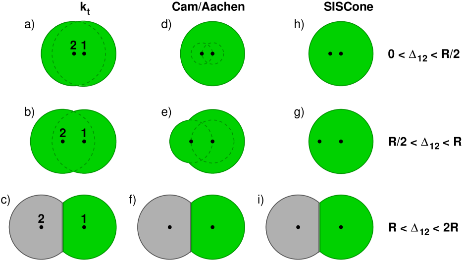
Let us now consider various cases. If $\Delta_{12}<R$, (Fig. 5.1a,b) the particles $p_{1}$ and $p_{2}$ will eventually end up in the same jet. The ghost will therefore belong to the jet irrespectively of having been clustered first with $p_{1}$ or $p_{2}$. The area of the jet will then be given by union of two circles of radius $R$, one centred on each of the two perturbative particles,

$$a_{k_{t},R}(\Delta_{12})=u\!\left(\frac{\Delta_{12}}{R}\right)\,{\pi R^{2}}\,,\qquad\qquad\mathrm{for}~{}\Delta_{12}<R\,,$$ (5.4)

where

$$u(x)=\frac{1}{\pi}\left[x\sqrt{1-\frac{x^{2}}{4}}+2\left(\pi-\arccos\left(\frac{x}{2}\right)\right)\right],$$ (5.5)

represents the area, divided by $\pi$, of the union of two circles of radius one whose centres are separated by $x$.

The next case we consider is $R<\Delta_{12}<2R$, Fig. 5.1c. In this case $p_{1}$ and $p_{2}$ will never be able to cluster together. Hence, they form different jets, and the ghost will belong to the jet of the closer of $p_{1}$ or $p_{2}$. The two jets will each have area

$$a_{k_{t},R}(\Delta_{12})=\frac{u\!\left(\Delta_{12}/R\right)}{2}\,\pi R^{2}\,,\qquad\qquad\mathrm{for}~{}R<\Delta_{12}<2R\,.$$ (5.6)

Finally, for $\Delta_{12}>2R$ the two jets formed by $p_{1}$ and $p_{2}$ each have area $\pi R^{2}$.

The three cases derived above are summarised in table 5.1 and plotted in Fig. 5.2.

It is interesting to note that the above results also illustrate the fact that for the $k_{t}$ algorithm, the passive area is equal to the Voronoi area. In this 2-particle configuration, the Voronoi diagram consists of a single line, equidistant between the two points, dividing the plane into two half-planes, each of which is the Voronoi cell of one of the particles (this is best seen in Fig. 5.1c). The intersection of the half-plane with the circle of radius $R$ centred on the particle has area ${\scriptstyle{\frac{1}{2}}}\pi R^{2}u(\Delta_{12}/R)$, and this immediately gives us the results Eqs. (5.4), (5.6) according to whether the particles cluster into a single jet or not.

Cambridge/Aachen.

Now we consider the behaviour of the Cambridge/Aachen jet algorithm [49, 50], also a sequential recombination algorithm, defined by the 2-particle distance measure $d_{ij}=\Delta_{ij}^{2}/R^{2}$ and beam-particle distance $d_{iB}=1$. Because in this case the distance measure does not involve the transverse momentum of the particles, the ghost only clusters first if $\min(\Delta_{1g},\Delta_{2g})<\Delta_{12}$. Otherwise, $p_{1}$ and $p_{2}$ cluster first into the jet $J$, and then $J$ captures the ghost if $\Delta_{Jg}\simeq\Delta_{1g}<R$.

The region $\Delta_{12}<R$ now needs to be separated into two parts, $\Delta_{12}<R/2$ and $R/2<\Delta_{12}<R$.

If the ghost clusters first, then it must have been contained in either of the dashed circles depicted in Figs. 5.1d,e. If $\Delta_{12}<R/2$ both these circles are contained in a circle of radius $R$ centred on $p_{1}$ (Fig. 5.1d), and so the jet area is $\pi R^{2}$.

If $R/2<\Delta_{12}<R$ (Fig. 5.1e) the circle of radius $\Delta_{12}$ centred on $p_{2}$ protrudes, and adds to the area of the final jet, so that

$${a_{\text{Cam},R}(\Delta_{12})}=w\!\left(\frac{\Delta_{12}}{R}\right)\,{\pi R^{2}}\,,\qquad\qquad\mathrm{for}~{}R/2<\Delta_{12}<R\,,$$ (5.7)

where

$$w(x)=\frac{1}{\pi}\left[\pi-\arccos\left(\frac{1}{2x}\right)+\sqrt{x^{2}-\frac{1}{4}}+x^{2}\arccos\left(\frac{1}{2x^{2}}-1\right)\right].$$ (5.8)

For $\Delta_{12}>R$ a Cambridge/Aachen jet has the same area as the $k_{t}$ jet, cf. Fig. 5.1f. As with the $k_{t}$ algorithm, the above results are summarised in table 5.1 and Fig. 5.2. The latter in particular illustrates the significant difference between the $k_{t}$ and Cambridge/Aachen areas for $\Delta_{12}\sim R/2$, caused by the different order of recombinations in the two algorithms.

SISCone.

Modern cone jet algorithms like SISCone identify stable cones and then apply a split/merge procedure to overlapping stable cones.

For $\Delta_{12}<R$ only a single stable cone is found, centred on $p_{1}$. Any ghost within distance $R$ of $p_{1}$ will therefore belong to this jet, so its area will be $\pi R^{2}$, cf. Fig. 5.1h,g.

For $R<\Delta_{12}<2R$ two stable cones are found, centred on $p_{1}$ and $p_{2}$. The split/merge procedure will then always split them, because the fraction of overlapping energy is zero. Any ghost falling within either of the two cones will be assigned to the closer of $p_{1}$ and $p_{2}$ (see Fig. 5.1i). The area of the hard jet will therefore be the same as for the $k_{t}$ and Cambridge algorithms.

Again these results are summarised in table 5.1 and Fig. 5.2 and one notices the large differences relative to the other algorithms at $R\lesssim 1$ and the striking feature that the cone algorithm only ever has negative corrections to the passive area for these energy-ordered two-particle configurations.

	$a_{\text{JA},R}(\Delta_{12})/\pi R^{2}$
	anti-$k_{t}$	$k_{t}$	Cambridge/Aachen	SISCone
$0<\Delta_{12}<R/2$	$1$	$u(\Delta_{12}/R)$	$1$	$1$
$R/2<\Delta_{12}<R$	$1$	$u(\Delta_{12}/R)$	$w(\Delta_{12}/R)$	$1$
$R<\Delta_{12}<2R$	$1$	$u(\Delta_{12}/R)\;/\;2$	$u(\Delta_{12}/R)\;/\;2$	$u(\Delta_{12}/R)\;/\;2$
$\Delta_{12}>2R$	$1$	$1$	$1$	$1$

Table 5.1: Summary of the passive areas for the three jet algorithms for the hard jet in an event containing one hard and one soft particle, separated by a $y$-$\phi$ distance $\Delta_{12}$. The functions $u$ and $w$ are defined in Eqs. (5.5) and (5.8).

Figure 5.2: Plot of the passive areas of the hard jet as a function of the distance between the hard and the soft particle, as given in table 5.1. The anti-$k_{t}$ case is not shown but corresponds to a constant line with $a(\Delta_{12})/(\pi R^{2})=1$.

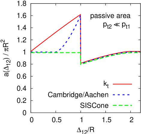
5.1.1.3 Area scaling violation

Given that jet passive areas are modified by the presence of a soft particle in the neighbourhood of a jet, one expects the average jet area to acquire a logarithmic dependence on the jet transverse momentum when the jets acquire a sub-structure as a consequence of radiative emission of gluons. To determine its coefficient we shall work in the approximation of small jet radii, motivated by the observation that corrections for finite $R$, proportional to powers of $R$, are usually accompanied by a small coefficient [124, 125].

In the small-angle limit, the QCD matrix element for the emission of the perturbative soft gluon, $p_{2}$, is

$$\frac{dP}{dp_{t2}\,d\Delta_{12}}=C_{1}\frac{2\alpha_{s}(p_{t2}\Delta_{12})}{\pi}\frac{1}{\Delta_{12}}\frac{1}{p_{t2}}\,,$$ (5.9)

where $C_{1}$ is $C_{F}$ or $C_{A}$ according to whether the hard particle $p_{1}$ is a quark or a gluon. We make use of the fact that $\Delta_{12}$ is just the angle between the two particles (to within a longitudinal boost-dependent factor), and will assume that $R$ is sufficiently small that the small-angle approximation is legitimate. The scale of the coupling is taken to be the transverse momentum of $p_{2}$ relative to $p_{1}$.

At order $\alpha_{s}$ the mean jet area with a given jet algorithm (JA) can be written

$$\langle a_{\text{JA},R}\rangle=a_{\text{JA},R}(0)+\langle\Delta a_{\text{JA},R}\rangle=\pi R^{2}+\langle\Delta a_{\text{JA},R}\rangle\,,$$ (5.10)

where we explicitly isolate the ${\cal O}\left(\alpha_{s}\right)$ higher-order contribution,

$$\langle\Delta a_{\text{JA},R}\rangle\simeq\int_{0}^{2R}d\Delta_{12}\int_{{Q_{0}}/\Delta_{12}}^{p_{t1}}dp_{t2}\frac{dP}{dp_{t2}\,d\Delta_{12}}(a_{\text{JA},R}(\Delta_{12})-a_{\text{JA},R}(0))\,,$$ (5.11)

with the $-a_{\text{JA},R}(0)$ term accounting for virtual corrections. $\left\langle\cdots\right\rangle$ represents therefore an average over perturbative emission. Note that because of the $1/p_{t2}$ soft divergence for the emission of $p_{2}$, Eq. (5.11) diverges unless one specifies a lower limit on $p_{t2}$ — accordingly we have to introduce an infrared cutoff ${Q_{0}}/\Delta_{12}$ on the $p_{t}$ of the emitted gluon. This value results from requiring that the transverse momentum of $p_{2}$ relative to $p_{1}$, i.e. $p_{t2}\Delta_{12}$, be larger than ${Q_{0}}$. The fact that we need to place a lower limit on $p_{t2}$ is an explicit manifestation of the fact that jet areas are infrared unsafe — they cannot be calculated order by order in perturbative QCD and for real-life jets they will depend on the details of non-perturbative effects (hadronisation). The case of the anti-$k_{t}$ jet algorithm is an exception since the area remains $\pi R^{2}$ independently of $\Delta_{12}$, hence the rhs of (5.11) vanishes independently of $Q_{0}$. In all other cases, one can account for this to some extent by leaving ${Q_{0}}$ as a free parameter and examining the dependence of the perturbative result on ${Q_{0}}$.

As concerns the finiteness of the $\Delta_{12}$ integration, all the jet algorithms we consider have the property that

$$\lim_{\Delta_{12}\to 0}a_{\text{JA},R}(\Delta_{12})=a_{\text{JA},R}(0)=\pi R^{2}\,;$$ (5.12a)

$$a_{\text{JA},R}(\Delta_{12})=\pi R^{2}\quad\mbox{for $\Delta_{12}>2R$}$$ (5.12b)

so that the integral converges for $\Delta_{12}\to 0$, and we can place the upper limit at $\Delta_{12}=2R$.

After evaluating Eq. (5.11), with the replacement $\Delta_{12}\to R$, both in the lower limit of the $p_{t2}$ integral and the argument of the coupling, we obtain

$$\langle\Delta a_{\text{JA},R}\rangle=d_{\text{JA},R}\frac{2\alpha_{s}C_{1}}{\pi}\ln\frac{Rp_{t1}}{{Q_{0}}}\;,\qquad d_{\text{JA},R}=\int_{0}^{2R}\frac{d\theta}{\theta}(a_{\text{JA},R}(\theta)-\pi R^{2})\,,$$ (5.13)

in a fixed coupling approximation, and

$$\langle\Delta a_{\text{JA},R}\rangle=d_{\text{JA},R}\frac{C_{1}}{\pi b_{0}}\ln\frac{\alpha_{s}({Q_{0}})}{\alpha_{s}(Rp_{t1})}\,,$$ (5.14)

with a one-loop running coupling, where $b_{0}=\frac{11C_{A}-2n_{f}}{12\pi}$. The approximation $\Delta_{12}\sim R$ in the argument of the running coupling in the integrand corresponds to neglecting terms of ${\cal O}\left(\alpha_{s}\right)$ without any enhancements from logarithms of $R$ or $p_{t1}/{Q_{0}}$.

The results for $d_{\text{JA},R}$ are

$$d_{\text{anti-}k_{t},R} =0,$$ (5.15a)

$$d_{k_{t},R} =\bigg{(}\frac{\sqrt{3}}{8}+\frac{\pi}{3}+\xi\bigg{)}R^{2}\,\simeq\,0.5638\,\pi R^{2}\,,$$ (5.15b)

$$d_{\text{Cam},R} =\bigg{(}\frac{\sqrt{3}}{8}+\frac{\pi}{3}-2\xi\bigg{)}R^{2}\,\simeq\,0.07918\,\pi R^{2}\,,$$ (5.15c)

$$d_{\text{SISCone},R} =\bigg{(}-\frac{\sqrt{3}}{8}+\frac{\pi}{6}-\xi\bigg{)}R^{2}\,\simeq\,-0.06378\,\pi R^{2}\,,$$ (5.15d)

where

$$\xi\equiv\frac{\psi^{\prime}(1/6)+\psi^{\prime}(1/3)-\psi^{\prime}(2/3)-\psi^{\prime}(5/6)}{48\sqrt{3}}\,\simeq\,0.507471\,,$$ (5.16)

with $\psi^{\prime}(x)=d^{2}/dx^{2}(\ln\Gamma(x))$. One notes that the coefficient for the $k_{t}$ algorithm is non-negligible, given that it is multiplied by the quantity $2\alpha_{s}C_{1}/\pi\ln Rp_{t1}/{Q_{0}}$ in Eq. (5.13) (or its running coupling analogue), which can be of order $1$. In contrast the coefficients for Cambridge/Aachen and SISCone are much smaller and similar (the latter being however of opposite sign). Thus $k_{t}$ areas will depend significantly more on the jet $p_{t}$ than will those for the other algorithms. In contrast, the soft-resilience of the anti-$k_{t}$ jet algorithm is manifest here with an area of $\pi R^{2}$ independently of $p_{t}$.

The fluctuation of the areas (over the emission $p_{2}$) can be calculated in a similar way. Let us define

$$\langle\sigma^{2}_{\text{JA},R}\rangle=\langle a_{\text{JA},R}^{2}\rangle-\langle a_{\text{JA},R}\rangle^{2}=\sigma^{2}_{\text{JA},R}(0)+\langle\Delta\sigma^{2}_{\text{JA},R}\rangle\,,\qquad\quad\sigma^{2}_{\text{JA},R}(0)=0\,,$$ (5.17)

where we have introduced $\sigma^{2}_{\text{JA},R}(0)$, despite its being null, so as to facilitate comparison with later results. We then evaluate

$$\langle\Delta\sigma^{2}_{\text{JA},R}\rangle=\langle\Delta a_{\text{JA},R}^{2}\rangle-\langle\Delta a_{\text{JA},R}\rangle^{2}\simeq\langle\Delta a_{\text{JA},R}^{2}\rangle\,,$$ (5.18)

where we neglect $\langle\Delta a_{\text{JA},R}\rangle^{2}$ since it is of ${\cal O}\left(\alpha_{s}^{2}\ln^{2}(Rp_{t1}/{Q_{0}})\right)$. The calculation of $\langle\Delta a_{\text{JA},R}^{2}\rangle$ proceeds much as for $\langle\Delta a_{\text{JA},R}\rangle$ and gives

$$\langle\Delta a_{\text{JA},R}^{2}\rangle=s_{\text{JA},R}^{2}\frac{C_{1}}{\pi b_{0}}\ln\frac{\alpha_{s}({Q_{0}})}{\alpha_{s}(Rp_{t1})}\;,\qquad s_{\text{JA},R}^{2}=\int_{0}^{2R}\frac{d\theta}{\theta}(a_{\text{JA},R}(\theta)-\pi R^{2})^{2}\,$$ (5.19)

for running coupling. The results are

$$s_{\text{anti-}k_{t},R}^{2} =0,$$ (5.20a)

$$s_{k_{t},R}^{2} =\bigg{(}\frac{\sqrt{3}\pi}{4}-\frac{19}{64}-\frac{15\zeta(3)}{8}+2\pi\xi\bigg{)}R^{4}\,\simeq\,(0.4499\,\pi R^{2})^{2}\,,$$ (5.20b)

$$s_{\text{Cam},R}^{2} =\bigg{(}\frac{\sqrt{3}\pi}{6}-\frac{3}{64}-\frac{\pi^{2}}{9}-\frac{13\zeta(3)}{12}+\frac{4\pi}{3}\xi\bigg{)}R^{4}\,\simeq\,(0.2438\,\pi R^{2})^{2}\,,$$ (5.20c)

$$s_{\text{SISCone},R}^{2} =\bigg{(}\frac{\sqrt{3}\pi}{12}-\frac{15}{64}-\frac{\pi^{2}}{18}-\frac{13\zeta(3)}{24}+\frac{2\pi}{3}\xi\bigg{)}R^{4}\,\simeq\,(0.09142\,\pi R^{2})^{2}\,.$$ (5.20d)

We have a hierarchy between algorithms that is similar to that observed for the average area scaling violations, with anti-$k_{t}$ showing no deviation from $\pi R^{2}$. The coefficient for Cambridge/Aachen is now more intermediate between the $k_{t}$ and SISCone values.

5.1.2 Active areas

5.1.2.1 Areas for 1-particle configurations and for ghost jets

This time, we consider a configuration with a single hard particle and an ensemble of ghosts, with the ghosts taking active part in the clustering.

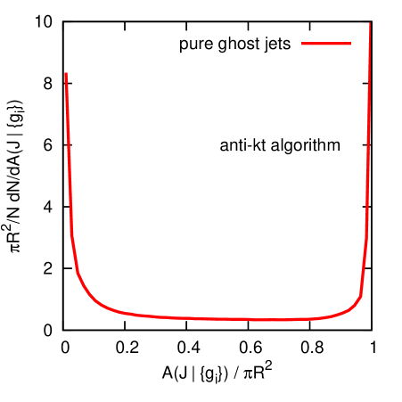
Figure 5.3: Distribution of the active area for pure-ghost jets obtained with the anti-$k_{t}$ algorithm.

Anti-$\boldsymbol{k_{t}}$.

The shortest anti-$k_{t}$ distance will be between the hard particle and either a ghost or the beam, depending on the pure geometrical distance. The hard particle $p_{1}$ will therefore cluster with all the ghosts within a geometrical distance $R$ from it before it becomes a jet (by clustering with the beam). Ghost–ghost distances are much larger, enhanced by a factor $p_{t}^{2}/g_{t}^{2}$. The active area will therefore be $\pi R^{2}$ (with no fluctuations), once again a direct consequence of the soft resilience of the anti-$k_{t}$ algorithm:

$$A_{\text{anti-}k_{t},R}(\text{one-particle-jet}) \,=\,\pi R^{2}\,,$$ (5.21a)

$$\Sigma_{\text{anti-}k_{t},R}(\text{one-particle-jet}) \,=\,0\,.$$ (5.21b)

Beside the hard jets, there will also be pure-ghost jets. Their distribution is most readily studied numerically, by directly clustering large numbers of ghost particles, with or without additional hard particles. Typically we add ghosts with a density $\nu_{g}$ of $\sim 100$ per unit area, in the rapidity region $|y|<y_{\text{max}}=6$, and study jets in the region $|y|<y_{\text{max}}-R$. This leads to about 7500 ghost particles. Each ghost is given a transverse momentum $\sim 10^{-100}\,\mathrm{GeV}$.

The resulting distribution of the anti-$k_{t}$ active areas $A(J\,|\,{\{g_{i}\}})$ is presented in Fig. 5.3 for a large ensemble of sets of ghosts. This distribution appears to be dominated by jets which are either almost circular and of area close to $\pi R^{2}$ and jets of much smaller area. We observe about 30% of the jets with an area smaller than $0.1\pi R^{2}$ and about 30% with an area larger than $0.95\pi R^{2}$. This distribution can be understood in the following way: pure-ghost jets will only be clustered once all the hard jets have been clustered. That clustering will start aggregating ghosts, giving them a larger $p_{t}$ than the other ghosts, seeding a process of further aggregating the ghosts in the vicinity of that original cluster, in a way similar to the clustering of the hard jets. This would give a peak close to $A=\pi R^{2}$. As this goes on, the space between the jets becomes smaller and small pure-ghost jets, of area close to 0, fill the spaces between the jets of area close to $\pi R^{2}$.

Note that this distribution justifies why anti-$k_{t}$ jets are not suited for the area–median estimation of the pileup density $\rho$. The patches used for pileup estimation would follow a distribution close to that of the pure-ghost jets — potentially with an additional bias coming from pileup fluctuations — and the large number of small jets would lead to a large uncertainty on the estimation of $\rho$.

Figure 5.4: Distribution of active areas for pure ghost jets and jets with a single hard particle: (a) $k_{t}$ algorithm, (b) Cambridge/Aachen algorithm.

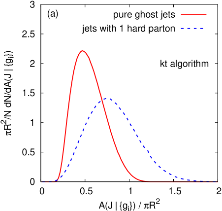
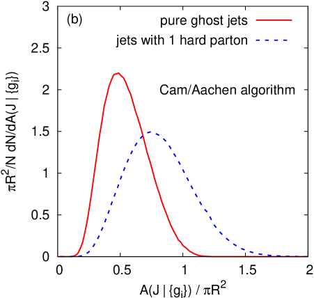
$\boldsymbol{k_{t}}$ and Cambridge/Aachen.

The active area for the $k_{t}$ and Cambridge/Aachen algorithms is again best studied numerically. On top of the ghosts distributed as discussed above, we added one hard particle with a transverse momentum of $100\,\mathrm{GeV}$ that we study. The results are insensitive to the transverse momentum as long as it is sufficiently larger than the ghost $p_{t}$. We briefly investigate in Appendix D.1 how the distribution of the “1-hard-parton” jet area gets modified when the transverse momentum of the parton is progressively reduced below the scale of a generic set of soft particles. Figure 5.4 shows the distribution of values of $A(J\,|\,{\{g_{i}\}})$ for pure ghost jets and jets with one hard particle. Let us concentrate initially on the case with a hard particle. Firstly, the average active area, Eq. (2.20) differs noticeably from the passive result of $\pi R^{2}$:

$$A_{k_{t},R}(\text{one-particle-jet}) \,\simeq\,0.812\,\pi R^{2}\,,$$ (5.22a)

$$A_{\text{Cam},R}(\text{one-particle-jet}) \,\simeq\,0.814\,\pi R^{2}\,.$$ (5.22b)

Secondly, the distributions of the area in Fig. 5.4 are rather broad. The randomness in the initial distribution of ghosts propagates all the way into the shape of the final jet and hence its area. This occurs because the $k_{t}$ and Cambridge/Aachen algorithms flexibly adapt themselves to local structure (a good property when trying to reconstruct perturbative showering), and once a random perturbation has formed in the density of ghosts this seeds further growth of the soft part of the jet. The standard deviations of the resulting distributions are

$$\Sigma_{k_{t},R}(\text{one-particle-jet}) \,\simeq\,0.277\,\pi R^{2}\,,$$ (5.23a)

$$\Sigma_{\text{Cam},R}(\text{one-particle-jet}) \,\simeq\,0.261\,\pi R^{2}\,.$$ (5.23b)

Figure 5.4 also shows the distribution of areas for pure ghost jets. One sees that pure ghost jets typically have a smaller area than hard-particle jets:

$$A_{k_{t},R}(\text{ghost-jet}) \,\simeq\,0.554\,\pi R^{2}\,,$$ (5.25a)

$$A_{\text{Cam},R}(\text{ghost-jet}) \,\simeq\,0.551\,\pi R^{2}\,,$$ (5.25b)

and the standard deviations are

$$\Sigma_{k_{t},R}(\text{ghost-jet}) \,\simeq\,0.174\,\pi R^{2}\,,$$ (5.26a)

$$\Sigma_{\text{Cam},R}(\text{ghost-jet}) \,\simeq\,0.176\,\pi R^{2}\,.$$ (5.26b)

The fact that pure ghost jets are smaller than hard jets has an implication for certain physics studies: one expects jets made of soft ‘junk’ (minimum bias, pileup, thermal noise in heavy ions) to have area properties similar to ghost jets; since they are smaller on average than true hard jets, the hard jets will emerge from the junk somewhat more clearly than if both had the same area.

SISCone.

The SISCone active area is amenable to analytical treatment, at least in some cases.

We recall that SISCone starts by finding all stable cones. A first stable cone is centred on the single hard particle. Additionally, there will be a large number of other stable cones, of order of the number of ghost particles added to the event [122]. In the limit of an infinite number of ghosts, all cones that can be drawn in the rapidity–azimuth plane and that do not overlap with the hard particle will be stable. Many of these stable cones will still overlap with the cone centred on the hard particle, as long as they do not contain the hard particle itself (see figure 5.5, left).

Figure 5.5: Left: the hard particle with the stable cone (H) centred on it, an example of a cone (A) that is unstable because it also contains the hard particle, and of two cones (B) and (C) that contain just ghost particles and are therefore stable. Right: some of the stable ghost cones (thin blue circles) that have the largest possible overlap with (H), together with the boundary of the hard jet after the split–merge procedure (dashed green line). In both diagrams, the grey background represents the uniform coverage of ghosts.

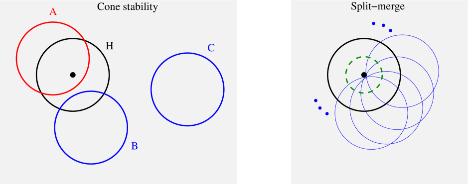
Next, the SISCone algorithm involves a split–merge procedure. One defines $\tilde{p}_{t}$ for a jet as the scalar sum of the transverse momenta of its constituents. During the split–merge step, SISCone finds the stable cone with the highest $\tilde{p}_{t}$, and then the next hardest stable cone that overlaps with it. To decide whether these two cones (protojets) are to be merged or split, it determines the fraction of the softer cone’s $\tilde{p}_{t}$ that is shared with the harder cone. If this fraction is smaller than some value $f$ (the overlap parameter of the cone algorithm), the two protojets are split: particles that are shared between them are assigned to the protojet to whose centre they are closer. Otherwise they are merged into a single protojet. This procedure is repeated until the hard protojet no longer has any overlap with other protojets. At this point it is called a jet, and the split–merge procedure continues on the remaining protojets (without affecting the area of the hard jet).

The maximum possible overlap fraction, $f_{\text{max}}$, between the hard protojet and a ghost protojet occurs in the situation depicted in figure 5.5 (right), i.e. when the ghost protojet’s centre is just outside the edge of the original hard stable cone (H). It is given by $f_{\text{max}}=2-u(1)=\frac{2}{3}-\frac{\sqrt{3}}{2\pi}\approx 0.391$. This means that for a split–merge parameter $f>f_{\text{max}}$ (commonly used values are $f=0.5$ and $f=0.75$) every overlap between the hard protojet and a pure-ghost stable cone will lead to a splitting. Since these pure-ghost stable cones are centred at distances $d>R$ from the hard particle, these splittings will reduce the hard jet to a circle of radius $R/2$ (the dashed green line in the right hand part of figure 5.5). The active area of the hard jet is thus

$$A_{\text{SISCone},R}(\text{one-particle-jet})=\frac{\pi R^{2}}{4}\,.$$ (5.27)

This result has been verified numerically using the same technique employed above for $k_{t}$ and Cambridge/Aachen.

Note that this area differs considerably from the passive area, $\pi R^{2}$. This shows that the cone area is very sensitive to the structure of the event, and it certainly does not always coincide with the naive geometrical expectation $\pi R^{2}$, contrary to assumptions sometimes made in the literature (see for example [131]).

We further note that in contrast to $k_{t}$ and Cambridge/Aachen algorithms, the SISCone algorithm always has the same active area for a single hard particle, independently of fluctuations of an infinitely dense set of ghosts, i.e.

$$\Sigma_{\text{SISCone},R}(\text{one-particle-jet})=0\,,$$ (5.28)

a property that SISCone shares with the anti-$k_{t}$ algorithm.

Figure 5.6: Distribution of pure-ghost jet areas for the SISCone algorithm, (a) with different values of the split–merge parameter $f$ and (b) different choices for the scale used in the split–merge procedure. Ghosts are placed on a grid up to $|y|<6$, with an average spacing of $0.2\times 0.2$ in $y$, $\phi$, and a random displacement of up to $\pm 0.1$ in each direction, and transverse momentum values that are uniform modulo a $\pm 5\%$ random rescaling for each ghost. We consider all jets with $y<5$. All jet definitions use $R=1$ and multiple passes.

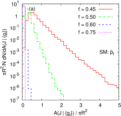
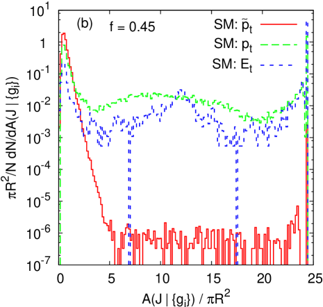
SISCone ghost-jet areas.

While the area of a hard particle jet could be treated analytically, this is not the case for the pure-ghost jet area. Furthermore, numerical investigations reveal that the pure-ghost area distribution has a much more complicated behaviour than for $k_{t}$ or Cambridge/Aachen. One aspect is that the distribution of pure-ghost jet areas is sensitive to the fine details of how the ghosts are distributed (density and transverse momentum fluctuations). Another is that it depends significantly on the details of the split–merge procedure. Figure 5.6a shows the distribution of areas of ghost jets for SISCone, for different values of the split–merge overlap threshold $f$. One sees, for example, that for smaller values of $f$ there are occasional rather large ghost jets, whereas for $f\gtrsim 0.6$ nearly all ghost jets have very small areas.

One of the characteristics of SISCone that differs from previous cone algorithms is the specific ordering and comparison variable used to determine splitting and merging. As explained above, the choice made in SISCone was $\tilde{p}_{t}$, the scalar sum of transverse momenta of all particles in a jet. Previous cone algorithms used either the vector sum of constituent transverse momenta, $p_{t}$ (an infrared unsafe choice), or the transverse energy $E_{t}=E\sin\theta$ (in a 4-vector recombination scheme). With both of these choices of variable, split–merge thresholds $f\lesssim 0.55$ can lead to the formation of ‘monster’ ghost jets, which can even wrap around the whole cylindrical phase space. For $f=0.45$ this is a quite frequent occurrence, as illustrated in figure 5.6b, where one sees a substantial number of jets occupying the whole of the phase space (i.e. an area $4\pi y_{\max}\simeq 24\pi R^{2}$). Monster jets can be formed also with the $\tilde{p}_{t}$ choice, though it is a somewhat rarer occurrence — happening in ‘only’ $\sim 5\%$ of events.

We have observed the formation of such monster jets also from normal pileup momenta simulated with Pythia [89, 90, 91], indicating that this disturbing characteristic is not merely an artefact related to our particular choice of ghosts. This indicates that a proper choice of the split–merge variable and threshold is critical in high-luminosity environments. The results from Figure 5.6a, suggest that if one wants to avoid monster jets, one has to choose a large enough value for $f$. Our recommendation is to adopt $f=0.75$ as a default value for the split–merge threshold (together with the use of the $\tilde{p}_{t}$ variable, already the default in SISCone, for reasons related to infrared safety and longitudinal boost invariance).

5.1.2.2 Areas for 2-particle configurations

In this section we study the same problem described in section 5.1.1.2, i.e. the area of jets containing two particles, a hard one and a softer (but still “perturbative”) one, Eq. (5.1), but now for active areas. As before, the results will then serve as an input in understanding the dependence of the active area on the jet’s transverse momentum when accounting for perturbative radiation.

Anti-$\boldsymbol{k_{t}}$.

With little surprise, the addition of the soft particle $p_{2}$ will not affect the area of the hard jet. The minimal anti-$k_{t}$ distance will be between particle $p_{1}$ and the closest of $p_{2}$ and the (remaining) ghosts, until that geometric distance reaches $R$ and the jet is clustered with the beam. The resulting area will be $\pi R^{2}$,

$$A_{\text{anti-}k_{t},R}(\Delta_{12})=\pi R^{2},$$ (5.29)

with no fluctuations

$$\Sigma_{\text{anti-}k_{t},R}(\Delta_{12})=0,$$ (5.30)

independently of the distance $\Delta_{12}$ between particles $p_{1}$ and $p_{2}$.

$\boldsymbol{k_{t}}$ and Cambridge/Aachen.

As was the case for the active area of a jet containing a single hard particle, we again have to resort to numerical analyses to study that of jets with two energy-ordered particles. We define $A_{\text{JA},R}(\Delta_{12})$ to be the active area for the energy-ordered two particle configuration already discussed in section 5.1.1.2.

Additionally since we have a distribution of areas for the single-particle active area case, it becomes of interest to study also $\Sigma_{\text{JA},R}(\Delta_{12})$ the standard deviation of the distribution of areas obtained for the two-particle configuration.

The results are shown in figure 5.7: the active areas can be seen to be consistently smaller than the passive ones, as was the case for the 1-particle area, but retain the same dependence on the angular separation between the two particles. Among the various features, one can also observe that the active area does not quite reach the single-particle value ($\simeq 0.81\pi R^{2}$) at $\Delta_{12}=2R$, but only somewhat beyond $2R$. This contrasts with the behaviour of the passive area. The figure also shows results for the cone area, discussed in the following subsection.

Figure 5.7: (a) Active areas (divided by $\pi R^{2}$) for the three jet algorithms as a function of the separation between a hard and a softer particle. For comparison we also include the passive areas, previously shown in Fig. 5.2. (b) The corresponding standard deviations.

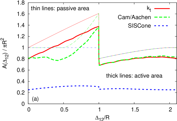
SISCone

In the case of the SISCone algorithm it is possible to find an analytical result for the two-particle active area, in an extension of what was done for one-particle case.

The stable-cone search will find one or two “hard” stable cones: the first centred on the hard particle and the second centred on the soft one, present only for $\Delta_{12}>R$. The pure-ghost stable cones will be centred at all positions distant by more than $R$ from both $p_{1}$ and $p_{2}$, i.e. outside the two circles centred on $p_{1}$ and $p_{2}$.

We shall consider the active area of the jet centred on the hard particle $p_{1}$. When $\Delta_{12}>R$, the jet centred on the soft particle has the same area.

Figure 5.8: Picture of the active jet area for 2-particle configurations in the case of the SISCone jet algorithm. The black points represent the hard (big dot) and soft (small dot) particles, the black circle is the hard stable cone. The final hard jet is represented by the shaded area. The left (a) (centre (b), right (c)) plot corresponds to $\Delta_{12}<R$ ($R<\Delta_{12}<\sqrt{2}R$, $\sqrt{2}R<\Delta_{12}<2R$).

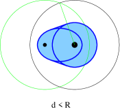
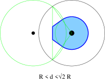
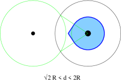
As in section 5.1.2.1, the split–merge procedure first deals with the pure-ghost protojets overlapping with the hard stable cone. For $f>f_{\text{max}}$, this again only leads to splittings. Depending of the value of $\Delta_{12}$, different situations are found as shown on figure 5.8. If the $y$-$\phi$ coordinates of the particles are $p_{1}\equiv(\Delta,0)$ and $p_{2}\equiv(0,0)$, the geometrical objects that are present are: the circle centred on $p_{1}$ with radius $R/2$; the tangents to this circle at $y$-$\phi$ coordinates $(\Delta_{12}/4,\pm\frac{1}{2}\sqrt{R^{2}-(\Delta_{12}/2)^{2}})$; and, for $\Delta_{12}<R$, the ellipse of eccentricity $\Delta_{12}/R$ whose foci are $p_{1}$ and $p_{2}$ (given by the equation, $\Delta_{a1}+\Delta_{a2}=R$, where $a$ is a point on the ellipse). For $\Delta_{12}<R$ the area of the jet is given by the union of the ellipse, the circle and the regions between the ellipse, the circle and each of the tangents (Fig. 5.8a). For $R<\Delta_{12}<\sqrt{2}R$ it is given by the circle plus the region between the circle, the two tangents and the line equidistant from $p_{1}$ and $p_{2}$ (Fig. 5.8b). For $\sqrt{2}R<\Delta_{12}<2R$ it is given by the circle plus the region between the circle and two tangents, up to the intersection of the two tangents (Fig. 5.8c). Finally, for $\Delta\geq 2R$, the area is $\pi R^{2}/4$.

An analytic computation of the active area gives

$$\frac{A_{\text{SISCone},R}(\Delta_{12})}{\pi R^{2}} = \frac{1}{4}\left[1-\frac{1}{\pi}\arccos\left(\frac{x}{2}\right)\right]$$

$$+ \begin{cases}\frac{x}{2\pi}\sqrt{1-\frac{x^{2}}{4}}+\frac{1}{4\pi}\sqrt{1-x^{2}}\arccos\left(\frac{x}{2-x^{2}}\right)&\Delta_{12}<R\\ \frac{x}{2\pi}\sqrt{1-\frac{x^{2}}{4}}-\frac{x}{8\pi}\frac{1}{\sqrt{1-\frac{x^{2}}{4}}}&R<\Delta_{12}\leq\sqrt{2}R\\ \frac{1}{2\pi x}\sqrt{1-\frac{x^{2}}{4}}&\sqrt{2}R<\Delta_{12}\leq 2R\end{cases}.$$

with $x=\Delta_{12}/R$, while for $\Delta_{12}>2R$, one recovers the result $\pi R^{2}/4$. The SISCone active area is plotted in figure 5.9 and it is compared to the results for $k_{t}$ and Cambridge/Aachen in figure 5.7. One notes that the SISCone result is both qualitatively and quantitatively much further from the passive result than was the case for $k_{t}$ and Cambridge/Aachen.

Figure 5.9: Active area of the hardest jet as a function of the distance between the hard and soft particle for the SISCone algorithm, cf. Eq. (5.1.2.2).

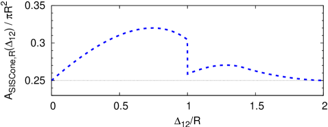
The main reason why the 2-point active area is larger than the 1-point active area (whereas we saw the opposite behaviour for the passive areas) is that the presence of the 2-particle configuration causes a number of the pure-ghost cones that were present in the 1-particle case to now contain the second particle and therefore be unstable. Since these pure ghost cones are responsible for reducing the jet area relative to the passive result (during the split–merge step), their absence causes the active area to be ‘less-reduced’ than in the 1-particle case.

5.1.2.3 Area scaling violation

We can write the order $\alpha_{s}$ contribution to the average active area in a manner similar to the passive area case, Eq. (5.11):

$$\langle A_{\text{JA},R}\rangle=A_{\text{JA},R}(0)+\langle\Delta A_{\text{JA},R}\rangle\,,$$ (5.32)

where we have used the relation $A_{\text{JA},R}(\text{one-particle-jet})\equiv A_{\text{JA},R}(0)$ and where

$$\langle\Delta A_{\text{JA},R}\rangle\simeq\int_{0}d\Delta_{12}\int_{{Q_{0}}/\Delta_{12}}^{p_{t1}}dp_{t2}\frac{dP}{dp_{t2}\,d\Delta_{12}}(A_{\text{JA},R}(\Delta_{12})-A_{\text{JA},R}(0))\,.$$ (5.33)

Note that compared to Eq. (5.11) we have removed the explicit upper limit at $2R$ on the $\Delta_{12}$ integral since, for active areas of some sequential recombination algorithms, $(A_{\text{JA},R}(\Delta_{12})-A_{\text{JA},R}(0))$ may be non zero even for $\Delta_{12}>2R$. Note also the notation for averages: we use $\left\langle\cdots\right\rangle$ to refer to an average over perturbative emissions, while $\left\langle\cdots\right\rangle_{g}$, implicitly contained in $A_{\text{JA},R}$ (see Eq. (2.20)), refers to an average over ghost ensembles. We now proceed as for the passive area scaling violations and write

$$\langle\Delta A_{\text{JA},R}\rangle\simeq D_{\text{JA},R}\frac{C_{1}}{\pi b_{0}}\ln\frac{\alpha_{s}({Q_{0}})}{\alpha_{s}(Rp_{t1})}\;,\qquad D_{\text{JA},R}=\int_{0}\frac{d\theta}{\theta}(A_{\text{JA},R}(\theta)-A_{\text{JA},R}(0))\,,$$ (5.34)

where for brevity we have given just the running-coupling result. One observes that the result continues to depend on $Q_{0}$, an indication that the active area is an infrared-unsafe quantity, just like the passive area. The coefficients for the anomalous dimension of the active area for the various algorithms are

$$D_{\text{anti-}k_{t},R} \simeq 0\,,$$ (5.35a)

$$D_{k_{t},R} \simeq 0.52\,\pi R^{2}\,,$$ (5.35b)

$$D_{\text{Cam},R} \simeq 0.08\,\pi R^{2}\,,$$ (5.35c)

$$D_{\text{SISCone},R} \simeq 0.1246\,\pi R^{2}\,,$$ (5.35d)

where the anti-$k_{t}$ and SISCone results has been obtained by integrating the analytical result, Eqs. (5.29) and (5.1.2.2) respectively, while the results for $k_{t}$ and Cambridge/Aachen have been obtained both by integrating the 2-point active-area results shown in Fig. 5.7 and by a direct Monte Carlo evaluation of Eq. (5.34). Note that while the coefficients for $k_{t}$ and Cambridge/Aachen are only slightly different from their passive counterparts, the one for SISCone has the opposite sign relative to the passive one.

The treatment of higher-order fluctuations of active areas is more complex than that for the passive ones, where the one-particle area was a constant. We can separate the fluctuations of active areas into two components, one (described above) that is the just the one-particle result and the other, $\langle\Delta\Sigma^{2}_{\text{JA},R}\rangle$, accounting for their modification in the presence of perturbative radiation:

$$\langle\Sigma^{2}_{\text{JA},R}\rangle=\Sigma^{2}_{\text{JA},R}(0)+\langle\Delta\Sigma^{2}_{\text{JA},R}\rangle\,,$$ (5.36)

where $\Sigma_{\text{JA},R}(0)$ is given by Eqs. (5.23a,b) for the $k_{t}$ and the Cambridge/Aachen algorithms respectively, and it is equal to zero for the anti-$k_{t}$ and SISCone algorithms. The perturbative modification $\langle\Delta\Sigma^{2}_{\text{JA},R}\rangle$ is itself now driven by two mechanisms: the fact that the second particle causes the average area to change, and that it also causes modifications of the fluctuations associated with the sampling over many ghost sets. We therefore write

$$\langle\Delta\Sigma^{2}_{\text{JA},R}\rangle \simeq S_{\text{JA},R}^{2}\frac{C_{1}}{\pi b_{0}}\ln\frac{\alpha_{s}({Q_{0}})}{\alpha_{s}(Rp_{t1})}\;,$$ (5.37)

$$\qquad S_{\text{JA},R}^{2} =\int_{0}\frac{d\theta}{\theta}\big{[}(A_{\text{JA},R}(\theta)-A_{\text{JA},R}(0))^{2}+\Sigma^{2}_{\text{JA},R}(\theta)-\Sigma^{2}_{\text{JA},R}(0)\big{]}\,$$ (5.38)

$$=\int_{0}\frac{d\theta}{\theta}(A^{2}_{\text{JA},R}(\theta)-A^{2}_{\text{JA},R}(0))-2A_{\text{JA},R}(0)D_{\text{JA},R}\,,$$ (5.39)

where as usual we neglect contributions that are not enhanced by any logarithm or that are higher-order in $\alpha_{s}$. The details of how to obtain these results are given in Appendix D.2.

The coefficient $S_{\text{JA},R}^{2}$ can be determined only numerically for the $k_{t}$ and Cambridge/Aachen algorithms, while for the SISCone algorithm the result can be deduced from Eq. (5.1.2.2) together with the knowledge that $\Sigma_{\text{SISCone},R}(\theta)\equiv 0$:

$${S}_{\text{anti-}k_{t},R}^{2} \simeq 0\,,$$ (5.40a)

$${S}_{k_{t},R}^{2} \simeq(0.41\,\pi R^{2})^{2}\,,$$ (5.40b)

$${S}_{\text{Cam},R}^{2} \simeq(0.19\,\pi R^{2})^{2}\,,$$ (5.40c)

$${S}_{\text{SISCone},R}^{2} \simeq(0.0738\,\pi R^{2})^{2}\,.$$ (5.40d)

Again, both the values and their ordering are similar to what we have obtained for the passive areas (see Eq. (5.20)).

5.1.2.4 $\boldsymbol{n}$-particle properties and large-$\boldsymbol{n}$ behaviour

Anti-$\boldsymbol{k_{t}}$ algorithm.

If we consider a situation with a single hard particle $p_{1}$, and multiple soft emissions $p_{i}$, $i\geq 2$, with $p_{t1}\gg p_{ti}$, the situation for the anti-$k_{t}$ jet areas does not change compared to what we have seen so far, with both the passive and active areas of the jet containing $p_{1}$ being simply $\pi R^{2}$. This is the main property of the anti-$k_{t}$ algorithm, namely that the hard (isolated) jets are circular. Beside the fact that this soft-resilience makes it a nice algorithm in an experimental framework, it also has important consequences when studying soft gluon emissions analytically in QCD. For example, the calculation of non-global logarithm contributions will be considerably simplified and the Milan factor will take the “universal” value, 1.49 for 3 active non-perturbative flavours.

In the limit where multiple particles are hard and become close to each other, the anti-$k_{t}$ areas can depart from $\pi R^{2}$. We shall comment a bit more on this below, when we discuss back-reaction.

$\boldsymbol{k_{t}}$ algorithm.

As for the passive area, the $k_{t}$ algorithm’s active area has the property that it can be expressed as a sum of individual particle areas:

$$A_{k_{t},R}(J)=\sum_{p_{i}\in J}A_{k_{t},R}(p_{i})\,.$$ (5.41)

This is the case because the presence of the momentum scale $k_{t}$ in the distance measure means that all ghosts cluster among themselves and with the hard particles, before any of the hard particles start clustering between themselves. However in contrast to the passive-area situation, there is no known simple geometrical construction for the individual particle area.

Equivalence of all areas for large $\boldsymbol{n}$

The existence of different area definitions is linked to the ambiguity in assigning ‘empty space’ to any particular jet. In the presence of a sufficiently large number of particles $n$, one expects this ambiguity to vanish because real particles fill up more and more of the empty space and thus help to sharpen the boundaries between jets. Thus in the limit of many particles, all sensible area definitions should give identical results for a given jet.

To quantify this statement, we examine (a bound on) the scaling law for the relation between the density of particles and the magnitude of the potential differences between different area definitions. We consider the limit of ‘dense’ coverage, defined as follows: take square tiles of some size and use them to cover the rapidity–azimuth cylinder (up to some maximal rapidity). Define $\lambda$ as the smallest value of tile edge-length such that all tiles contain at least one particle. In an event consisting of uniformly distributed particles, $\lambda$ is of the same order of magnitude as the typical inter-particle distance. The event is considered to be dense if $\lambda\ll R$.

Now let us define a boundary tile of a jet to be a tile that contains at least one particle of that jet and also contains a particle from another jet or has an adjacent tile containing one or more particle(s) belonging to a different jet. We expect that the difference between different jet-area definitions cannot be significantly larger than the total area of the boundary tiles for a jet.

The number of boundary tiles for jets produced by a given jet algorithm (of radius $R$) may scale in a non-trivial manner with the inter-particle spacing $\lambda$, since the boundary may well have a fractal structure. We therefore parametrise the average number of boundary tiles for a jet, $N_{b,\text{JA},R}$ as

$$N_{b,\text{JA},R}\sim\left(\frac{R}{\lambda}\right)^{{\!\daleth}_{\,\text{JA}}},$$ (5.42)

where the fractal dimension ${\!\daleth}_{\,\text{JA}}=1$ would correspond to a smooth boundary. The total area of these boundary tiles gives an upper limit on the ambiguity of the jet area

$$\langle|a_{\text{JA},R}-A_{\text{JA},R}|\rangle\lesssim N_{b,\text{JA},R}\,\lambda^{2}\sim R^{{\!\daleth}_{\,\text{JA}}}\lambda^{2-{\!\daleth}_{\,\text{JA}}}\,,$$ (5.43)

and similarly for the difference between active or passive and Voronoi areas. As long as ${\!\daleth}_{\,\text{JA}}<2$ the differences between various area definitions are guaranteed to vanish in the infinitely dense limit, $\lambda\to 0$. We note that ${\!\daleth}_{\,\text{JA}}=2$ corresponds to a situation in which the boundary itself behaves like an area, i.e. occupies the same order of magnitude of space as the jet itself. This would be visible in plots representing jet active areas (such as Fig. 2.2), in the form of finely intertwined jets. We have seen no evidence for this and therefore believe that $1\leq{\daleth}_{\,\text{JA}}<2$ for all three jet algorithms considered here.

In practice we expect the difference between any two area definitions to vanish much more rapidly than Eq. (5.43) as $\lambda\to 0$, since the upper bound will only be saturated if, for every tile, the difference between two area definitions has the same sign. This seems highly unlikely. If instead differences in the area for each tile are uncorrelated (but each of order $\lambda^{2}$) then one would expect to see

$$\langle|a_{\text{JA},R}-A_{\text{JA},R}|\rangle\sim\sqrt{N_{b,\text{JA},R}}\,\lambda^{2}\sim R^{{\!\daleth}_{\,\text{JA}}/2}\lambda^{2-{\!\daleth}_{\,\text{JA}}/2}\,.$$ (5.44)

We have measured the fractal dimension for the $k_{t}$ and Cambridge/Aachen algorithms and find ${\daleth}_{\,k_{t}}\simeq{\!\daleth}_{\,\text{Cam}}\simeq 1.20-1.25$. Note that any measurement of the fractal dimension of jet algorithms in real data would be severely complicated by additional structure added to jets by QCD branching, itself also approximately fractal in nature.

The fact that active and passive (or Voronoi) areas all give the same result in dense events has practical applications in real-life situations where an event is populated by a very large number of particles (heavy ion collisions being an example). In this case it will be possible to choose the area type which is fastest to compute (for instance the Voronoi area) and use the results in place of the active or passive one.

5.1.3 Back reaction

So far we have considered how a set of infinitely soft ghosts clusters with a hard jet, examining also cases where the jet has some finitely-soft substructure. This infinitely-soft approximation for the ghosts is not only adequate, but also necessary from the point of view of properly defining jet areas. However if we are to understand the impact of pileup and underlying-event radiation on jet finding — the original motivation for studying areas — then we should take into account the fact that these contributions provide a dense background of particles at some small but finite soft scale $\sim\Lambda_{QCD}$.

This has two main consequences. The first (more trivial) one is that pileup or underlying event can provide an alternative, dynamic infrared cutoff in the $p_{t2}$ integration in equations such as Eq. (5.11): assuming that the density of PU transverse momentum per unit area is given by $\rho$ then one can expect that when $p_{t2}\ll\pi R^{2}\rho$, the presence of $p_{2}$ will no longer affect the clustering of the ghosts (i.e. the PU particles). In this case the $p_{t2}$ integral will then acquire an effective infrared cutoff $\sim\pi R^{2}\rho$ and in expressions such as Eqs. (5.13,5.14), $Q_{0}$ will be replaced by $\pi R^{3}\rho$. Note that neither with infinitely nor finitely-soft ghosts do we claim control over the coefficient in front of this cutoff, though we do have confidence in the prediction of its $R$ dependence for small $R$.

The second consequence of the finite softness of the PU contribution is that the addition of the PU particles can modify the set of non-PU particles that make it into a jet. This is the effect we called back reaction in our introductory discussion (see Section 2.2).

That back reaction should happen is quite intuitive since it concerns non-PU particles whose softness is commensurate with the PU scale. However the extent to which it occurs depends significantly on the jet algorithm. Furthermore for some algorithms it can also occur (rarely) even for non-PU particles that are much harder than the PU scale.

As with the studies of areas, there are two limits that can usefully be examined for back-reaction: the illustrative and mathematically simpler (but less physical) case of a pointlike minimum-bias background and the more realistic case with diffuse pileup radiation.

5.1.3.1 Back reaction from pointlike minimum-bias

Let us first calculate back reaction in the case of pointlike minimum bias. We will consider minimum-bias particles with transverse momentum $p_{tm}$ distributed uniformly on the $y$–$\phi$ cylinder with density $\nu_{m}\ll 1$. We use a subscript $m$ rather than $g$ to differentiate them from ghost particles, the key distinction being that $p_{tm}$ is small but finite, where $p_{tg}$ is infinitesimal.

We thus consider the situation in which a particle $p_{1}$, with large transverse momentum, $p_{t1}\gg p_{tm}$, has emitted a soft particle $p_{2}$ on a scale commensurate with the minimum-bias particles, $p_{t2}\sim p_{tm}$. We shall calculate the probability that $p_{2}$ was part of the jet in the absence of the minimum-bias particle, but is lost from it when the minimum-bias particle is added. This can be written

$$\frac{dP^{(\text{loss})}_{\text{JA},R}}{dp_{t2}}=\int d\phi_{m}dy_{m}\nu_{m}\int d\Delta_{12}\frac{dP}{dp_{t2}\,d\Delta_{12}}H_{\text{JA},R}(p_{2}\in J_{1})\,H_{\text{JA},R}(p_{2}\notin J_{1}|\,p_{m})\,,$$ (5.45)

where $H_{\text{JA},R}(p_{2}\in J_{1})$ is $1$ ($0$) if, in the absence of $p_{m}$, $p_{2}$ is inside (outside) the jet that contains $p_{1}$. Similarly, $H_{\text{JA},R}(p_{2}\notin J_{1}|p_{m})$ is $1$ ($0$) if, in the presence of $p_{m}$, $p_{2}$ is outside (inside) the jet that contains $p_{1}$. One can also define the probability for $p_{2}$ to not be part of the jet in the absence of the minimum-bias particle, but to be gained by the jet when the minimum-bias particle is added,

$$\frac{dP^{(\text{gain})}_{\text{JA},R}}{dp_{t2}}=\int d\phi_{m}dy_{m}\nu_{m}\int d\Delta_{12}\frac{dP}{dp_{t2}\,d\Delta_{12}}H_{\text{JA},R}(p_{2}\notin J_{1})\,H_{\text{JA},R}(p_{2}\in J_{1}|\,p_{m})\,.$$ (5.46)

It is convenient to factor out the particle production probability as follows, in the small $R$ limit,

$$\frac{dP^{(\text{loss,gain})}_{\text{JA},R}}{dp_{t2}}=\left.\Delta_{12}\frac{dP}{dp_{t2}\,d\Delta_{12}}\right|_{\Delta_{12}=R}\nu_{m}\;b^{(\text{loss,gain})}_{\text{JA},R}(p_{t2}/p_{tm})\,,$$ (5.47)

where $b^{(\text{loss})}_{\text{JA},R}(p_{t2}/p_{tm})$ ($b^{(\text{gain})}_{\text{JA},R}(p_{t2}/p_{tm})$) can be thought of as the effective ‘back-reaction area’ over which the minimum-bias particle causes a loss (gain) of jet contents, given a $d\Delta_{12}/\Delta_{12}$ angular distribution for the jet contents:

$$b^{(\text{loss})}_{\text{JA},R}(p_{t2}/p_{tm}) =\int d\phi_{m}dy_{m}\int\frac{d\Delta_{12}}{\Delta_{12}}H_{\text{JA},R}(p_{2}\in J_{1})\,H_{\text{JA},R}(p_{2}\notin J_{1}|\,p_{m})\,,$$ (5.48)

$$b^{(\text{gain})}_{\text{JA},R}(p_{t2}/p_{tm}) =\int d\phi_{m}dy_{m}\int\frac{d\Delta_{12}}{\Delta_{12}}H_{\text{JA},R}(p_{2}\notin J_{1})\,H_{\text{JA},R}(p_{2}\in J_{1}|\,p_{m})\,.$$ (5.49)

Let us first consider the $k_{t}$ and Cambridge/Aachen sequential-recombination algorithms for which the $H$ functions in Eqs. (5.48,5.49) translate to a series of $\Theta$-functions, e.g.

$$H_{k_{t},R}(p_{2}\in J_{1})H_{k_{t},R}(p_{2}\notin J_{1}|\,p_{m})=\Theta(R-\Delta_{12})\Theta(R-\Delta_{2m})\Theta(\Delta_{1(2+m)}-R)\times\\ \times\Theta(\Delta_{1m}-\min(1,p_{t2}/p_{tm})\Delta_{2m})\Theta(\Delta_{12}-\min(1,p_{tm}/p_{t2})\Delta_{2m})\,,$$ (5.50)

for the $k_{t}$ algorithm and

$$H_{\text{Cam},R}(p_{2}\in J_{1})H_{\text{Cam},R}(p_{2}\notin J_{1}|\,p_{m})=\Theta(R-\Delta_{12})\Theta(R-\Delta_{2m})\Theta(\Delta_{1(2+m)}-R)\times\\ \times\Theta(\Delta_{1m}-\Delta_{2m})\Theta(\Delta_{12}-\Delta_{2m})\,,$$ (5.51)

for Cambridge/Aachen, where $\Delta_{1(2+m)}$ is the distance between $p_{1}$ and the recombined $p_{2}+p_{m}$. Evaluating integrals with the above $\Theta$-functions is rather tedious, but one can usefully consider the limit $p_{tm}\ll p_{t2}\ll p_{t1}$. This of physical interest because it relates to the probability that the minimum-bias particle induces changes in jet momentum that are much larger than $p_{tm}$, and a number of simplifications occur in this limit. Since

$$\Delta_{1(2+m)}=\left|\vec{\Delta}_{12}+\frac{p_{tm}}{p_{t2}+p_{tm}}\vec{\Delta}_{2m}\right|=\Delta_{12}+\frac{p_{tm}}{p_{t2}}\frac{\vec{\Delta}_{12}\cdot\vec{\Delta}_{2m}}{\Delta_{12}}+{\cal O}\left(\frac{p_{tm}^{2}}{p_{t2}^{2}}R\right)\,,$$ (5.52)

$p_{2}$ must be close to the edge of the jet in order for it to be pulled out by $p_{m}$, $|\Delta_{12}-R|\ll 1$. Without loss of generality, we can set $y_{1}=\phi_{1}=\phi_{2}=0$, so that $\Delta_{12}=y_{2}\simeq R$, and

$$\Delta_{1(2+m)}=y_{2}+\frac{p_{tm}}{p_{t2}}(y_{m}-R)+{\cal O}\left(\frac{p_{tm}^{2}}{p_{t2}^{2}}R\right).$$ (5.53)

We can then carry out the integrations over $\phi_{m}$ and $y_{2}$ straightforwardly, leading to following the result for loss at high $p_{t2}$,

$$b^{(\text{loss})}_{k_{t},R}(p_{t2}/p_{tm}\gg 1)\simeq b^{(\text{loss})}_{\text{Cam},R}(p_{t2}/p_{tm}\gg 1)\simeq\int_{R}^{2R}dy_{m}\,\frac{(y_{m}-R)}{R}\frac{p_{tm}}{p_{t2}}\,2\sqrt{R^{2}-(y_{m}-R)^{2}}=\frac{2}{3}\frac{p_{tm}}{p_{t2}}R^{2}\,.$$ (5.54)

For the anti-$k_{t}$ algorithm it is tempting to follow the same path, i.e. to impose that the loss term is obtained by clustering $p_{m}$ with $p_{2}$ in order to pull $p_{2}$ out of the jet, and write the $H$ functions (for the loss term and assuming $p_{t2}\gg p_{tm}$) as

$$\Theta(R-\Delta_{12})\,\Theta(\Delta_{1(2+m)}-R)\,\Theta(\Delta_{1m}-(p_{t1}/p_{t2})\Delta_{2m})\,\Theta(\Delta_{12}-(p_{t1}/p_{t2})\Delta_{2m})\,\Theta(R-\Delta_{2m})\,.$$ (5.55)

In the limit of interest, $p_{tm}\ll p_{t2}\ll p_{t1}$, the constraint that $p_{2}$ must be in the jet and that $p_{2}+p_{m}$ must be outside the jet imposes, as before (see (5.53)), that $\Delta_{12}$ must be between $R-\frac{p_{tm}}{p_{t2}}(y_{m}-R)$ and $R$. But now, the condition that $p_{2}$ clusters with $p_{m}$ and not $p_{1}$ (the fourth term in (5.55)) imposes that $p_{m}$ lies within a half-circle of radius $Rp_{t2}/p_{t1}$ centred on $p_{2}$. Ultimately, this gives a contribution proportional to $\frac{p_{t2}^{2}p_{tm}}{p_{t1}^{3}}R^{2}$ which, as we shall show below, is subleading for the case of interest, $p_{t2}\ll p_{t1}$.

Instead, the dominant contribution comes from the situation where $p_{m}$ clusters with $p_{1}$ and the recoil causes $p_{2}$ to fall outside the jet, giving

$$H_{{\rm anti-}k_{t},R}(p_{2}\in J_{1})H_{{\rm anti-}k_{t},R}(p_{2}\notin J_{1}|\,p_{m})=\Theta(R-\Delta_{12})\Theta(\Delta_{(1+m)2}-R)\times\\ \times\Theta(\Delta_{1m}-\Delta_{12})\Theta(\Delta_{12}-\min(p_{t1}/p_{t2},p_{t1}/p_{tm})\Delta_{2m})\Theta(R-\Delta_{1m})\,.$$ (5.56)

In the limit $p_{t1}\gg p_{t2},p_{tm}$, the recoil (along the direction $\vec{\Delta}_{12}$) is found to be $p_{tm}/p_{t1}y_{m}$ and this ultimately leads to

$$b^{(\text{loss})}_{\text{anti-}k_{t},R}\simeq\frac{2}{3}\frac{p_{tm}}{p_{t1}}R^{2}\,,$$ (5.57)

i.e. suppressed by a factor $p_{t2}/p_{t1}$ compared to the result obtained in (5.54) for the $k_{t}$ and Cambridge/Aachen algorithms. Note also that, contrary to the results for the $k_{t}$ and Cambridge/Aachen algorithms, (5.57) is valid independently of the ordering between $p_{t2}$ and $p_{tm}$, as long as they are both small compared to $p_{t1}$.

In a similar manner we obtain for the gain,

$$b^{(\text{gain})}_{k_{t},R}(p_{t2}/p_{tm}\gg 1)\simeq b^{(\text{gain})}_{\text{Cam},R}(p_{t2}/p_{tm}\gg 1)\simeq\int_{R/2}^{R}dy_{m}\,\frac{(R-y_{m})}{R}\frac{p_{tm}}{p_{t2}}\,2\sqrt{R^{2}-(R-y_{m})^{2}}=\\ =\left(\frac{2}{3}-\frac{\sqrt{3}}{4}\right)\frac{p_{tm}}{p_{t2}}R^{2}\,.$$ (5.58)

and for the anti-$k_{t}$ algorithm,

$$b^{(\text{gain})}_{\text{anti-}k_{t},R}\simeq b^{(\text{loss})}_{\text{anti-}k_{t},R}\simeq\frac{2}{3}\frac{p_{tm}}{p_{t1}}R^{2}\,,$$ (5.59)

Figure 5.10: The effective area for back-reaction as a function of the ratio of the soft perturbative scale $p_{t2}$ and the point-like minimum-bias scale $p_{tm}$, showing separately the loss (left) and gain (right) components for four jet definitions. For the anti-$k_{t}$ results, we have set $p_{t1}=100\,p_{t2}$. The thin black dotted lines represent our analytic results valid for $p_{t2}\gg p_{tm}$.

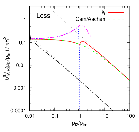
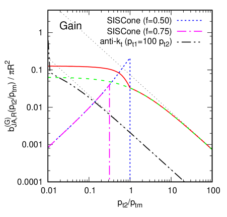
The SISCone results are included and have the property that

$$b^{(\text{loss})}_{\text{SISCone},R}(p_{t2}/p_{tm}) =0\quad\text{for}\quad\frac{p_{t2}}{p_{tm}}>\frac{f}{1-f}\,,$$ (5.60a)

$$b^{(\text{gain})}_{\text{SISCone},R}(p_{t2}/p_{tm}) =0\quad\text{for}\quad\frac{p_{t2}}{p_{tm}}>\frac{1-f}{f}\,.$$ (5.60b)

i.e. at high $p_{t2}$, point-like minimum bias never induces back-reaction in the cone algorithm.

The results for general $p_{t2}/p_{tm}$, determined numerically, are shown in figure 5.10. On sees that our analytic estimates work very well in the region where $p_{t2}\gg p_{tm}$ and that indeed, the anti-$k_{t}$ algorithm has a suppressed back reaction and SISCone has zero back-reaction at large $p_{t2}$ as expected. On the other hand, for $p_{t2}\sim p_{tm}$ back-reaction is more likely with the cone algorithm — the effective area over which the MB particle can cause a change in jet contents is $\sim 0.5\pi R^{2}$, to be compared to $\sim 0.1\pi R^{2}$ for the $k_{t}$ and Cambridge/Aachen algorithms.

One may use the results Eqs. (5.54)–(5.60) to determine the average change in jet-momentum due to back reaction. Because of the logarithmic spectrum of emissions $dP/(dp_{t2}\,d\Delta_{12})$, one finds that it receives contributions from the whole logarithmic region $p_{tm}<p_{t2}<p_{t1}$,

$$\langle\Delta p_{t,\text{JA},R}^{(\text{gain}-\text{loss})}\rangle\simeq\int_{p_{tm}}^{p_{t1}}dp_{t2}\,p_{t2}\left[\frac{dP^{(\text{gain})}_{\text{JA},R}}{dp_{t2}}-\frac{dP^{(\text{loss})}_{\text{JA},R}}{dp_{t2}}\right]=\beta_{\text{JA},R}\,\rho\cdot\frac{C_{1}}{\pi b_{0}}\ln\frac{\alpha_{s}(p_{tm}R)}{\alpha_{s}(p_{t1}R)}\,,$$ (5.61)

(evaluated for running coupling), where $\rho=\nu_{m}p_{tm}$ corresponds to the average transverse momentum of minimum-bias radiation per unit area and

$$\beta_{\text{JA},R}=\lim_{p_{t2}\to\infty}\frac{p_{t2}}{p_{tm}}\left(b^{(\text{gain})}_{\text{JA},R}(p_{t2}/p_{tm})-b^{(\text{loss})}_{\text{JA},R}(p_{t2}/p_{tm})\right)\,.$$ (5.62)

The structure of the correction in Eq. (5.61) is very similar to that for the actual contamination from minimum bias, $\rho\langle\Delta a_{\text{JA},R}\rangle$, with $\langle\Delta a_{\text{JA},R}\rangle$ as determined in section 5.1.1.3: notably, for fixed coupling, the average back-reaction scales with the logarithm of the jet $p_{t}$. The coefficients $\beta_{\text{JA},R}$,

$$\beta_{k_{t},R}=\beta_{\text{Cam},R} =-\frac{\sqrt{3}}{4}R^{2}\simeq-0.1378\pi R^{2}\,,$$ (5.63a)

$$\beta_{\text{anti-}k_{t},R}=\beta_{\text{SISCone},R} =0\,.$$ (5.63b)

can be directly compared to the results for the $d_{\text{JA},R}$ there. The values are relatively small, similar in particular to what one observes for the Cambridge/Aachen algorithm, though of opposite sign. Note also that for the SISCone and anti-$k_{t}$ algorithms, one would expect a contribution similar to (5.61), proportional to $\rho$, but without the logarithmic enhancement, although, in the case of the anti-$k_{t}$ algorithm, further cancellations could happen since $b^{(\text{gain})}_{\text{anti-}k_{t},R}\simeq b^{(\text{loss})}_{\text{anti-}k_{t},R}$.

Though the average change in jet momentum, both from scaling violations of the area and from back-reaction, have a similar analytical structure, it is worth bearing in mind that these similar analytical structures come about quite differently in the two cases. Regarding area scaling violations, a significant fraction of jets, $\sim\alpha_{s}\ln p_{t1}/p_{tm}$, are subject to a change in area $\sim R^{2}$ (cf. section 5.1.1.3), and a consequent modification of the minimum-bias contamination by a modest amount $\sim p_{tm}$. In contrast the average back reaction effect $\sim\alpha_{s}p_{tm}\ln p_{t1}/p_{tm}$, is due to large modifications of the jet momentum $\sim p_{t2}$ with $p_{tm}\ll p_{t2}\ll p_{t1}$ occurring rarely, with a differential probability that depends on $p_{t2}$ as $\sim\alpha_{s}dp_{t2}p_{tm}/p_{t2}^{2}$. One consequence of this is that the mean square change in transverse momentum due to back-reaction is dominated by very rare modifications of jets in which $p_{t2}\sim p_{t1}$, giving

$$\left\langle\left(\Delta p_{t,\text{JA},R}^{(\text{gain,loss})}\right)^{2}\right\rangle\sim\alpha_{s}p_{t1}p_{tm}\nu_{m}\,.$$ (5.64)

Note that the coefficient of this dispersion is non-zero even for the SISCone algorithm, due to the residual probability $\sim p_{tm}/p_{t1}$ that it has, for finite $p_{t1}$, for any change in structure with $p_{tm}\ll p_{t2}\lesssim p_{t1}$. For the anti-$k_{t}$ algorithm, one would also obtain the behaviour given by Eq. (5.64) since, for $p_{t2}\sim p_{t1}$, the gain and loss probabilities also behave as $\sim\alpha_{s}dp_{t2}p_{tm}/p_{t2}^{2}$.

5.1.3.2 Back reaction from diffuse pileup

Let us now examine back reaction in the case where the minimum-bias radiation has a uniform diffuse structure, consisting of a high density of pileup particles, $\nu_{m}\gg 1$. The relation between back reaction in the point-like and diffuse cases is rather similar to the relation between passive and active areas: key analytical features remain unaffected by the change in the structure of the soft background, but certain specific coefficients change.

We define the probability for loss in the presence of diffuse PU as

$$\frac{dP^{(\text{loss})}_{\text{JA},R}}{dp_{t2}}=\mathop{\lim_{\nu_{m}\to\infty}}_{\rho=\nu_{m}\langle p_{tm}\rangle\>\text{fixed}}\left\langle\int d\Delta_{12}\frac{dP}{dp_{t2}\,d\Delta_{12}}H_{\text{JA},R}(p_{2}\in J_{1})\,H_{\text{JA},R}(p_{2}\notin J_{1}|\,\rho)\right\rangle_{\mathrm{PU}},$$ (5.65)

where the average is performed over the ensemble of PU configurations, and now $H_{\text{JA},R}(p_{2}\notin J_{1}|\,\rho)$ is 1 (0) if $p_{2}$ is outside (inside) the jet containing $p_{1}$ in the presence of the specific pileup instance. A similar equation holds for the gain probability.

Then, as with Eq. (5.47) we factorise this,

$$\frac{dP^{(\text{loss})}_{\text{JA},R}}{dp_{t2}}=\left.\Delta_{12}\frac{dP}{dp_{t2}\,d\Delta_{12}}\right|_{\Delta_{12}=R}\;B^{(\text{loss})}_{\text{JA},R}(p_{t2}/\rho)\,,$$ (5.66)

into one piece related to the probability for perturbative emission and a second piece $B^{(\text{loss})}_{\text{JA},R}$ that is the diffuse analogue of the effective back-reaction area $b^{(\text{loss})}_{\text{JA},R}$ in the point-like case. Note however that it is not so obvious exactly what geometrical area $B^{(\text{loss})}_{\text{JA},R}$ actually corresponds to. Similarly, we introduce $dP^{(\text{gain})}_{\text{JA},R}/dp_{t2}$ and $B^{(\text{gain})}_{JA,R}$ corresponding to the gain in the presence of a diffuse PU.

As for the point-like case, we can obtain analytical results for $B^{(\text{loss,gain})}_{\text{JA},R}(p_{t2}/\rho)$ in the case of the SISCone algorithm, for which (with $f>f_{\max}\simeq 0.391$)

$$B^{(\text{loss})}_{\text{SISCone},R}(p_{t2}/\rho)=B^{(\text{gain})}_{\text{SISCone},R}(p_{t2}/\rho)=0\,.$$ (5.67)

This is a consequence of the facts (a) that the addition of a uniform background of PU particles has no effect on the stability (or instability) of a specific cone, (b) that for $p_{t2}\ll p_{t1}$ the split–merge step is immaterial to the jet finding if $p_{2}$ is within the cone around $p_{1}$, and (c) that for $p_{2}$ outside the cone around $p_{1}$, the maximal possible overlap is of $p_{2}$’s stable cone with that of $p_{1}$ is $f_{\max}$ and if $f>f_{\max}$ then the two cones will always be split, ensuring that $p_{2}$ remains in a jet distinct from $p_{1}$. We believe that real-life corrections to the zero in Eq. (5.67) are proportional to the standard deviation, $\sigma$, of PU transverse-momentum density from point to point in the event.

Figure 5.11: Numerical results for the diffuse effective back-reaction ‘area’, $B^{(\text{loss,gain})}_{\text{JA},R}(p_{t2}/\rho)$, for the $k_{t}$ and Cambridge/Aachen algorithms, with the point-like results $b^{(\text{loss,gain})}_{\text{JA},1}(p_{t2}/p_{tm})$ shown for comparison also. Results obtained for $R=1$ and verified also for $R=0.7$.

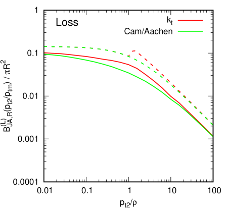
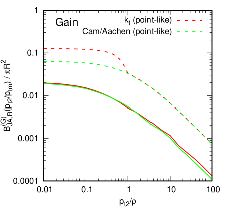
Numerical results for the $B^{(\text{loss,gain})}_{\text{JA},R}(p_{t2}/\rho)$ for the $k_{t}$ and Cambridge/Aachen algorithms are given in figure 5.11 and compared to the results in the point-like case. One sees that the general functional form is rather similar though the normalisations are somewhat smaller (by a factor of $2$ for loss, a factor $\sim 10$ for gain). The asymptotic large-$p_{t2}$ behaviours are observed to be

$$B^{(\text{loss})}_{k_{t},R}(p_{t2}/\rho)\simeq B^{(\text{loss})}_{\text{Cam},R}(p_{t2}/\rho) \simeq 0.11\,\pi R^{2}\,\frac{\rho}{p_{t2}}$$ (5.68a)

$$B^{(\text{gain})}_{k_{t},R}(p_{t2}/\rho)\simeq B^{(\text{gain})}_{\text{Cam},R}(p_{t2}/\rho) \simeq 0.013\,\pi R^{2}\,\frac{\rho}{p_{t2}}$$ (5.68b)

The case of the anti-$k_{t}$ algorithm is slightly more delicate. With a uniform background, the momentum imbalance, due to the background within a distance $R$ of $p_{1}$ clustered instead with particle $p_{2}$, will be of order $\pi/2\,R^{2}\rho\,(p_{t2}/p_{t1})^{2}$, with a corresponding recoil of order $\pi/2\,R^{3}\,(\rho/p_{t1})(p_{t2}/p_{t1})^{2}$. This means that one would obtain

$$B^{(\text{loss})}_{\text{anti-}k_{t},R}(p_{t2}/\rho)\simeq B^{(\text{gain})}_{\text{anti-}k_{t},R}(p_{t2}/\rho)\simeq\frac{1}{2}\frac{\pi R^{2}\rho}{p_{t1}}\frac{p_{t2}^{2}}{p_{t1}^{2}}.$$ (5.69)

One should however also notice that, as for SISCone, one should expect corrections proportional to the PU fluctuations $\sigma$ which, as for the point-like case, should be proportional to $\pi R^{2}\sigma/p_{t1}$. For $p_{t2}\ll p_{t1}$ the latter is expected to be the dominant behaviour.

As in the point-like case we can calculate the mean change in jet transverse momentum due to back reaction and we obtain

$$\langle\Delta p_{t,\text{JA},R}^{(\text{gain}-\text{loss})}\rangle\simeq\int_{p_{tm}}^{p_{t1}}dp_{t2}p_{t2}\left[\frac{dP^{(\text{gain})}_{\text{JA},R}}{dp_{t2}}-\frac{dP^{(\text{loss})}_{\text{JA},R}}{dp_{t2}}\right]={\mathcal{B}}_{\text{JA},R}\,\rho\cdot\frac{C_{1}}{\pi b_{0}}\ln\frac{\alpha_{s}(\rho R^{3})}{\alpha_{s}(p_{t1}R)}\,,$$ (5.70)

with

$${\mathcal{B}}_{\text{JA},R}=\lim_{p_{t2}\to\infty}\frac{p_{t2}}{\rho}\left(B^{(\text{gain})}_{\text{JA},R}(p_{t2}/\rho)-B^{(\text{loss})}_{\text{JA},R}(p_{t2}/\rho)\right)\,.$$ (5.71)

Even though $b^{(\text{loss,gain})}_{\text{JA},R}$ had $p_{t2}/p_{tm}$ as its argument and $B^{(\text{loss,gain})}_{\text{JA},R}$ has $p_{t2}/\rho$, the final expressions for the average back-reaction in the point-like and diffuse cases, Eqs. (5.61), (5.70), have almost identical forms — in particular the overall scale appearing in each is $\rho$ and the only difference appears in the denominator for the argument of the logarithm. The coefficients are slightly smaller,

$${\mathcal{B}}_{k_{t},R}={\mathcal{B}}_{\text{Cam},R} \simeq-0.10\pi R^{2}\,,$$ (5.72a)

$${\mathcal{B}}_{\text{SISCone},R}={\mathcal{B}}_{\text{anti-}k_{t},R} =0\,,$$ (5.72b)

and will again translate into modest effects compared to the overall pileup contamination in the jets. Note however that in general the scaling with $R$ of $b^{(\text{loss,gain})}_{k_{t},R}(p_{t2}/p_{tm})$ and $B^{(\text{loss,gain})}_{k_{t},R}(p_{t2}/\rho)$ is subtly different. The former truly behaves like an area, in that $b^{(\text{loss,gain})}_{k_{t},R}(p_{t2}/p_{tm})/R^{2}$ is $R$-independent; the latter instead has the property that it is $B^{(\text{loss,gain})}_{k_{t},R}(R^{2}p_{t2}/\rho)$ that is $R$-independent.

Finally, as for the case of the point-like background, the diffuse PU will lead to a mean square change of the jet due to back-reaction which will be dominated by rare modifications with $p_{t2}\sim p_{t1}$ such that

$$\left\langle\left(\Delta p_{t,\text{JA},R}^{(\text{gain,loss})}\right)^{2}\right\rangle\sim\alpha_{s}p_{t1}\rho\,.$$ (5.73)

This is also true for the anti-$k_{t}$ algorithm since the extra suppression factor become finite for $p_{t2}\sim p_{t1}$.

5.1.4 Comparison to Monte-Carlo simulations

In this section we examine the properties of jet areas in the context of realistic events, as simulated with Herwig [60, 61] and Pythia [89, 90, 91]. There are two purposes to doing so. Firstly we wish to illustrate the extent to which the simple single-gluon emission arguments of the previous section hold once one includes full parton-showering and hadronisation. Secondly, jet areas play an important role in the estimation and subtraction of underlying event and pileup contamination. The study of jet areas in realistic events can help to highlight some of the issues that arise in such a procedure.

Figure 5.12: Distribution of active and passive areas of the two hardest jets in a range of simulated LHC dijet events, with a minimum $p_{t}$ of $1\,\mathrm{TeV}$ in the Pythia event generation (v6.4, default tune). Only jets with $|y|<2$ have been included in the histogram; ‘parton’ indicates parton-level, ‘hadron’ indicates hadron-level with the UE switched off, ‘UE’ corresponds to hadron-level with UE switched on and in the ‘pileup’ case the UE-level event is supplemented with additional pileup events corresponding to $0.25\,\mathrm{mb}^{-1}$ per bunch crossing ($\sim 25$ simultaneous interactions). For all jet algorithms we use $R=1$. A ghost area $\simeq 0.02$ was used throughout except for SISCone, where the ghost area was roughly $0.1$ in the active area cases. Note that “area” in these plots corresponds to $a_{\text{JA},R}(J_{i})$ and $A_{\text{JA},R}(J_{i})$ respectively for the passive and active areas. As such the latter has been averaged over ghost ensembles (see Eq. (2.20)) and the dispersion is a consequence of the event and jet structure. We have found that $5$ ghost ensembles were sufficient for $k_{t}$ and Cambridge/Aachen algorithms, and $3$ for SISCone (with pileup, 1 ensemble would actually have been enough). In contrast, the Cam/Aachen 1-particle jet result corresponds to $\pi R^{2}/NdN/dA(\text{1-particle-jet}|\{g_{i}\})$ and serves to illustrate how the impact of variability in the event structure in real events has consequences rather similar to that of the variability of ghost-particle ensembles in the theoretical arguments of the previous sections.

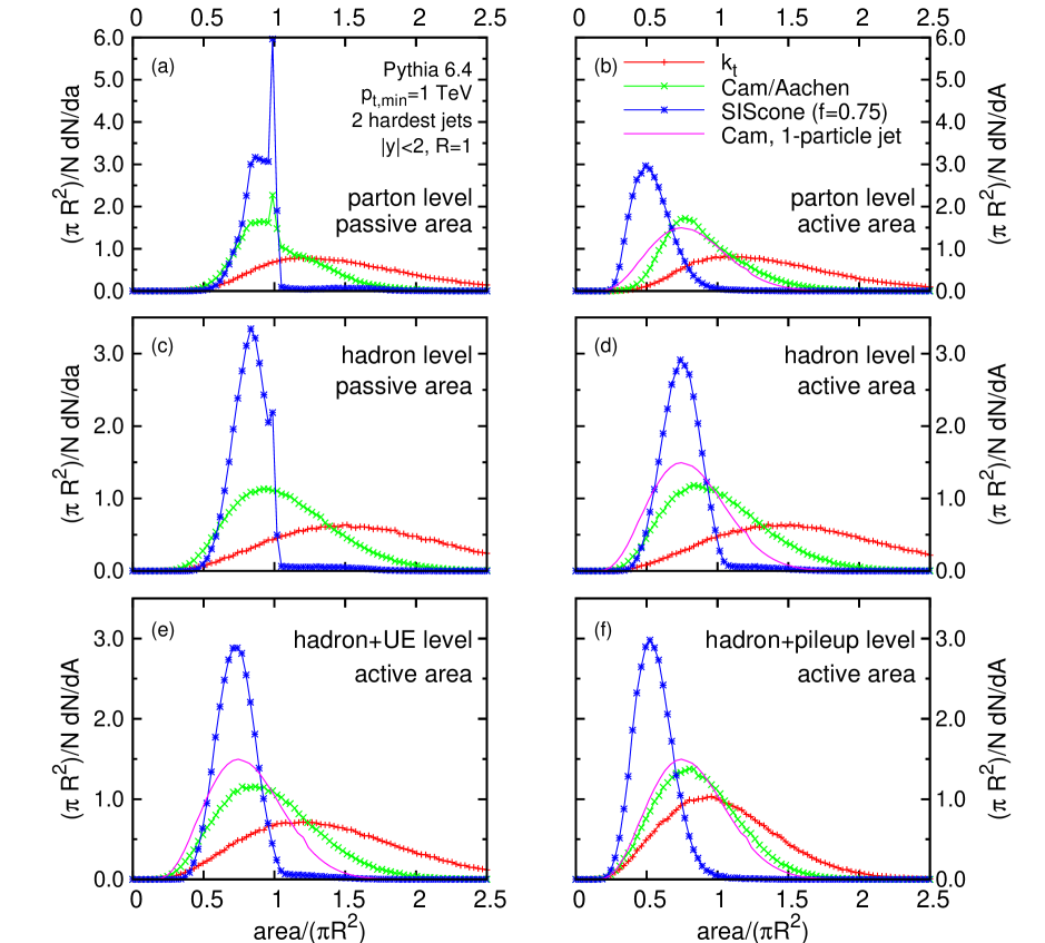
Let us start with an investigation of the distribution of the areas of hard jets with $p_{t}\gtrsim 1\,\mathrm{TeV}$ in simulated LHC dijet events, and first concentrate on the $k_{t}$, Cambridge/Aachen and SISCone algorithms. The area distributions are shown on Fig. 5.12 for various ‘levels’ in the Monte Carlo: just after parton showering, after hadronisation, both with and without an UE, and finally with a pileup contribution corresponding to a luminosity of 0.25 mb^-1 per bunch crossing (i.e. $\mu\sim 25$). We examine both passive and active areas.

The passive areas distributions at parton-shower level, Fig. 5.12a, are those that are most amenable to understanding in terms of our analytical results. Firstly one notes that the SISCone and Cambridge/Aachen algorithms have a clear peak at $a=\pi R^{2}$. These two algorithms both have the property (cf. section 5.1.1.2) that the area is not affected by moderately collinear ($\Delta_{12}<R$ for SISCone, $\Delta_{12}<R/2$ for Cambridge/Aachen) soft particle emission. Thus it is possible, even in the presence of parton showering (which is mostly collinear), for the passive area to remain $\pi R^{2}$. For the cone algorithm, the other main structure is a “shoulder” region $0.8\lesssim a/(\pi R^{2})\lesssim 1$, which coincides nicely with the range of values that can be induced by 2-particle configurations (cf. Fig. 5.2). A similar shoulder exists for the Cambridge algorithm, which however additionally has jets with $a>\pi R^{2}$ — again the range of values spanned, up to $a\simeq 1.6\pi R^{2}$, is rather similar to what would be expected from the two-particle calculations. Further broadening of these distributions at the edges is attributable to parton-level states with more than two particles. In contrast the parton-level passive area distribution for the $k_{t}$ algorithm seems less directly related to the $2$-particle calculations of section 5.1.1.2. This can be understood by observing that the $k_{t}$ passive area is modified even by rather collinear emissions, and the multiple collinear emissions present in parton showers add together to cause substantial broadening of the area distribution.

At parton shower level, there are relatively few particles in the event and there is no obvious boundary to the jet — the ghosts that we add provide a way of assigning that empty area. It is therefore not surprising to see significant differences between the two ways of adding ghosts, i.e. the passive and active area distributions. This is most marked for SISCone, as is to be expected from the results of section 5.1.2.1, which showed that for a 1-particle jet the active area is $\pi R^{2}/4$. There is a trace of this result in Fig. 5.12b, where one sees that the SISCone distribution now extends down to $A=\pi R^{2}/4$. There is however no peak structure, presumably because even a highly collinear emission gives a slight modification of the area, cf. Fig. 5.9 (the same argument given for the absence of a peak for the passive $k_{t}$ area). For the Cambridge/Aachen and $k_{t}$ algorithms, there is less difference between active and passive area distributions, again as expected.

As one moves to events with more particles, for example hadron level, Fig. 5.12c and d, the particles themselves start to give a clearer outline to the jets. Thus the passive and active distributions are far more similar. This is less so for SISCone than the others, as is to be expected, for which one still sees a trace of the peak at $a=\pi R^{2}$ for the passive area.

For events with many particles, for example with the UE (Fig. 5.12e) and then pileup (Fig. 5.12f) added, the difference between passive and active area distributions is so small that we show only the active area result. These last two plots are the most relevant to phenomenology. A feature of both is that the dispersion is smallest for SISCone (but significantly different from zero) and largest for $k_{t}$, precisely as one would expect from Eqs. (5.36) and (5.40). Another feature is how for Cambridge/Aachen the dispersion is essentially that associated with $\Sigma(0)$, the distribution being very similar to the 1-parton active area result, shown as the solid line. This similarity is strongest when there is pileup: the logarithmic enhancement that enters in Eq. (5.37) is reduced because the pileup introduces a large value for $Q_{0}\sim 20\,\mathrm{GeV}$. In this case even the $k_{t}$ algorithm starts to have a distribution of areas that resembles the $1$-parton active area result, and for SISCone one once again sees signs of the lower limit at $A=\pi R^{2}/4$, the one-particle active area result.

Figure 5.13: Distributions obtained in the same context as for Fig. 5.12, this time for the anti-$k_{t}$ algorithm. We just show the two extreme situations, corresponding to parton-level (blue lines) and hadron level with pileup (red lines). We show the distributions for two different jet minimum transverse momentum: 100 GeV (solid lines) and 1 TeV (dotted lines).

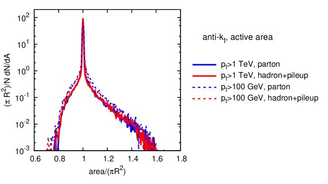
Let us now move to area distributions for the anti-$k_{t}$ algorithm. A few representative distributions are plotted in Fig. 5.13. Only the active area distribution is plotted for the two extreme particle multiplicities — the “parton” level and the “hadron+pileup” level — and for two jet transverse momenta. Most often, the jet area comes out as $\pi R^{2}$ as expected from our analytic studies so far. The use of a logarithmic scale on the vertical axis on Fig. 5.13 allows one to highlight the rare tails away from $\pi R^{2}$, occurring for about 1% of the jets. These features are stable when we add pileup to the event of vary the jet $p_{t}$, showing that jet areas are constrained by the hard structure of the event.

Figure 5.14: The mean (solid line) and standard deviation (band) of the active area for each of the two hardest jets in $qq\to qq$ and $gg\to gg$ events simulated with Herwig 6.5, as a function of the jet transverse momentum. The theory curves (thick dashed for mean, thin dashed for standard deviation) correspond to Eqs. (5.32)–(5.40) with a 1-loop coupling ($\Lambda_{\mathrm{QCD}}=0.2\,\mathrm{GeV}$, $n_{f}=5$), and $Q_{0}$ fitted (for the mean values). The areas have been obtained with ghosts of size $0.02$ for anti-$k_{t}$, $k_{t}$ and Cambridge/Aachen, and $0.1$ for SISCone. For all algorithms, we used $R=1$. Note that the horizontal scale is uniform in $\ln\ln p_{t}/\Lambda$. We considered $pp$ collisions with $\sqrt{s}=14\,\mathrm{TeV}$.

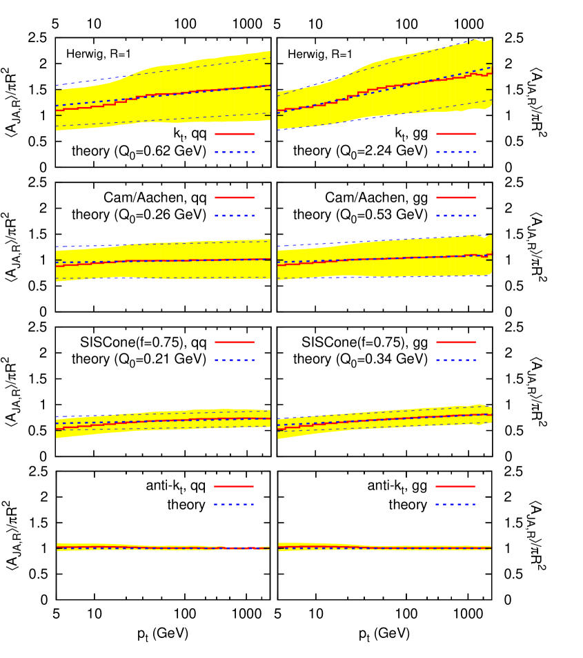
While the plots of Figs. 5.12 and 5.13 provide an illustration of many of the features that we have discussed in the earlier sections of this Chapter, the fact that we have not systematically calculated area distributions means that the discussion necessarily remains qualitative. For quantitative checks, one should instead examine the mean active area and its dispersion and compare them to the results of section 5.1.2. This is done in Fig. 5.14, separately for $qq\to qq$ and for $gg\to gg$ scattering, as a function of the jet transverse momentum. The horizontal scale has been chosen uniform in $\ln\ln p_{t}/\Lambda$ so that our predictions correspond to straight lines.

The predictions of section 5.1.2 set the slope of those lines for each algorithm, and the agreement is reasonable in all cases. The infrared cutoff scale $Q_{0}$ is not predicted, and may differ both between quark and gluon jets and between algorithms. The values for $Q_{0}$ have therefore been fitted, using the results for the mean, and are consistent with a general non-perturbative origin (modulo issues in SISCone discussed below). The standard deviation (indicated by the band for the Monte Carlo simulation and the thin dashed lines for the theory result) is then entirely predicted, and also agrees remarkably well. Thus, overall, our simple analytical calculations provide a surprisingly successful picture of the mean and dispersions for various algorithms, over a range of jet transverse momenta. This is all the more striking considering that the calculation is based on just the first term in a series $\alpha_{s}^{n}\ln^{n}p_{t}$, and is in part based on a small angle approximation.

Some remarks are due regarding the $Q_{0}$ values. Clear patterns emerge: it is largest for $k_{t}$, smallest for SISCone, and systematically larger for gluon jets than for quark jets. In the case of SISCone with quark jets, the value is uncomfortably close to the value of $\Lambda_{QCD}=0.2\,\mathrm{GeV}$ used in the one-loop coupling. It may be that this low value is an artefact whose origin lies in the finite density both of actual event particles and of ghosts (the latter due to speed limitations in SISCone): when one has a limited density of particles and/or ghosts, the measured area may be intermediate between the passive and “ideal” active areas; because SISCone has such a large difference between passive and active areas (a factor of 4 for the 1-particle results), the finite density effects can be significant, and so $Q_{0}$ may be taking an extreme value in order to compensate for this.

Compared to $k_{t}$, Cambridge/Aachen and SISCone, the anti-$k_{t}$ algorithm shows an area very close to $\pi R^{2}$ with almost no dependence on $p_{t}$ and a very small dispersion.

A final comment concerns the choice of event generator. Here we have shown results from Herwig (v. 6.5). Pythia with the original shower (the default choice in v. 6.4) is known to have difficulties reproducing anomalous dimensions associated with soft large angle radiation [132, 133], whereas the new shower [134] mostly resolves these issues [133]. Similar concerns are potentially relevant here too. In our original studies [29], we actually found that both Pythia showers give results similar to Herwig’s (and ours) in all cases except the $k_{t}$ algorithm, for which both Pythia showers give a slope a factor of two smaller than expected. This suggests that an experimental measure of the $p_{t}$ dependence of jet areas might provide some non-trivial constraints on parton-showering dynamics.

5.1.5 Summary

The concept of a jet area is one that initially seems rather intuitive. Yet, as we have seen both in Chapter 2 (in particular in Section 2.3) and in this Chapter, there is a wealth of physics associated with it, both in terms of how one defines it and as concerns the interplay between a jet’s internal structure and its area. This is reflected in the range of quantities that can be studied to characterise the behaviour of jet areas, summarised in table 5.2.

Our guiding principle in defining jet areas has been that they should provide a measure of a jet’s susceptibility to additional underlying event and pileup radiation, in the limit in which these are infinitely soft. Two opposite hypotheses for the structure of such radiation, pointlike or diffuse, lead to two definitions of the area, respectively passive or active, both calculated in practice with the help of infinitely soft “ghost” particles. The two definitions can be used with any infrared safe jet algorithm, and we have studied them both with sequential recombination algorithms (anti-$k_{t}$, $k_{t}$ and Cambridge/Aachen) and with a stable-cone with split–merge algorithm, SISCone.

The area of a jet may depend on its substructure. For the simplest case of a jet made of a single hard particle, the passive area coincides with one’s naive expectation of $\pi R^{2}$ for all jet algorithms considered here. The active area — that related to the more realistic, diffuse picture for UE and pileup — instead differs from $\pi R^{2}$, except for the anti-$k_{t}$ algorithm. The most surprising result is that for SISCone, whose active area is $\pi R^{2}/4$, a consequence of the split–merge dynamics (the midpoint algorithm widely used at the Tevatron behaves similarly). Thus the widespread assumption that cone-based algorithms automatically have an area of $\pi R^{2}$ is, in many cases, unjustified.

Real jets of course consist of more than a single particle. The first level of substructure involves the addition of a soft particle to the neighbourhood of the jet. For all except the anti-$k_{t}$ algorithm, we have seen that this modifies the jet area, and that the average jet area then becomes an infrared unsafe quantity. Even if it looks like a bad feature at first sight, the infrared unsafety of jet areas is actually desirable and tightly related to the fact that areas are meant to precisely measure the jet’s susceptibility to soft radiation. In that respect, the soft resilience of the anti-$k_{t}$ algorithm corresponds to an area remaining $\pi R^{2}$ when we add any number of soft particles to the jet. Also, the small pileup contamination often observed with the SISCone algorithm can be related to its smaller catchment area than that of recombination algorithms.

From our analytic viewpoint, it emerges that the effects of gluon emission can usefully be summarised in terms of an anomalous dimension, which encodes how the jet’s average area depends on its transverse momentum. We have calculated this to leading order and seen that it agrees remarkably well with the $p_{t}$ dependence of measures of the jet areas in hadron-level Monte Carlo simulations.

quantity	discussed in	description
Passive area	Section 5.1.1	single-ghost area
$\bullet$ average area
$a$(1PJ)	Sect. 5.1.1.1	passive area for a 1-particle jet
$\langle a\rangle$	Eq. (5.10)	average passive area of jets with QCD branching:
		$\langle a\rangle=a(\mathrm{1PJ})+d\,\frac{C_{1}}{\pi b_{0}}\ln\frac{\alpha_{s}(Q_{0})}{\alpha_{s}(Rp_{t})}+\ldots$
$d$	Eq. (5.15)	coefficient of leading scaling violations of $\langle a\rangle$
$\bullet$ area fluctuations
$\sigma^{2}(\mathrm{1PJ})$		variance of one-particle passive area (0 by definition)
$\langle\sigma^{2}\rangle$	Eq. (5.17)	variance of passive area of jets with QCD branching:
		$\langle\sigma^{2}\rangle=\sigma^{2}(\mathrm{1PJ})+s^{2}\,\frac{C_{1}}{\pi b_{0}}\ln\frac{\alpha_{s}(Q_{0})}{\alpha_{s}(Rp_{t})}+\ldots$
$s^{2}$	Eq. (5.20)	coefficient of leading scaling violations of $\langle\sigma^{2}\rangle$
Active area	Section 5.1.2	many-ghost area (ghosts also cluster among themselves)
$\bullet$ average area
$A$(1PJ)	(5.21,5.22,5.27)	active area for a 1-particle jet
$\langle A\rangle$	Eq. (5.32)	average active area of jets with QCD branching:
		$\langle A\rangle=A(\mathrm{1PJ})+D\,\frac{C_{1}}{\pi b_{0}}\ln\frac{\alpha_{s}(Q_{0})}{\alpha_{s}(Rp_{t})}+\ldots$
$D$	Eq. (5.35)	coefficient of leading scaling violations of $\langle A\rangle$
$A$(GJ)	Eq. (5.25)	average active area for pure-ghost jets
$\bullet$ area fluctuations
$\Sigma^{2}(\mathrm{1PJ})$	(5.21,5.23,5.28)	variance of one-particle active area
$\langle\Sigma^{2}\rangle$	Eq. (5.36)	variance of active area of jets with QCD branching:
		$\hskip 8.5359pt\langle\Sigma^{2}\rangle=\Sigma^{2}(\mathrm{1PJ})+S^{2}\,\frac{C_{1}}{\pi b_{0}}\ln\frac{\alpha_{s}(Q_{0})}{\alpha_{s}(Rp_{t})}+\ldots$
$S^{2}$	Eq. (5.40)	coefficient of leading scaling violations of $\langle\Sigma^{2}\rangle$
$\Sigma^{2}$(GJ)	Eq. (5.26)	variance of active area for pure-ghost jets
Back reaction	Section 5.1.3	action of finite-momentum min-bias (MB) on the clustering of the non-MB particles
$\bullet$ pointlike MB
$dP^{(L,G)}/dp_{t2}$	Eqs. (5.45, 5.46)	probability of jet losing (L) or gaining (G) $p_{t2}$ worth
		of non-MB particles
$b^{(L,G)}(p_{t2}/p_{tm})$	Eqs. (5.48, 5.49)	eff. area for loss, gain (MB particle has $\perp$ mom. $p_{tm}$)
$\beta$	Eq. (5.62)	coeff. of net high-$p_{t2}$ gain$-$loss: $\lim_{p_{t2}\to\infty}\frac{p_{t2}}{p_{tm}}b^{(G-L)}(\frac{p_{t2}}{p_{tm}}\!)\!$
$\bullet$ diffuse MB
$dP^{(L,G)}/dp_{t2}$	Eq. (5.65)	probability of jet losing (L) or gaining (G) $p_{t2}$ worth
		of non-MB particles
$B^{(L,G)}(p_{t2}/\rho)$	Eq. (5.66)	eff. area for loss, gain (MB has $\perp$-mom. density $\rho$)
$\cal B$	Eq. (5.71)	coeff. of net high-$p_{t2}$ gain$-$loss: $\lim_{p_{t2}\to\infty}\frac{p_{t2}}{\rho}B^{(G-L)}(\frac{p_{t2}}{\rho}\!)\!$

Table 5.2: A summary of the mathematical quantities defined throughout this article, together with descriptions of the associated physical concepts.

	$a$(1PJ)	$A$(1PJ)	$\sigma$(1PJ)	$\Sigma$(1PJ)	$d$	$D$	$s$	$S$	A(GJ)	$\Sigma$(GJ)
$k_{t}$	$1$	$0.81$	$0$	$0.28$	$\,\,0.56$	$0.52$	$0.45$	$0.41$	$0.55$	$0.17$
Cam/Aachen	$1$	$0.81$	$0$	$0.26$	$\,\,0.08$	$0.08$	$0.24$	$0.19$	$0.55$	$0.18$
anti-$k_{t}$	$1$	$0$	$0$	$0$	$\,\,0$	$0$	$0$	$0$	—	—
SISCone	$1$	$1/4$	$0$	$0$	$\!\!-0.06$	$0.12$	$0.09$	$0.07$	—	—

Table 5.3: A summary of the numerical results for the main quantities worked out in the article and described in table 5.2. All results are normalised to $\pi R^{2}$, and rounded to the second decimal figure. Anomalous dimensions multiply powers of $\alpha_{s}^{n}\ln^{n}p_{t}/Q_{0}$ that for typical jet transverse momenta sum to something of order $1$. Active-area and anomalous-dimension results hold only in the small-$R$ limit, though finite-$R$ corrections are small. Back reaction is not easily summarised by a single number, and the reader is therefore referred to Figs. 5.10, 5.11.

A summary of our main results for active and passive areas, their fluctuations and their anomalous dimensions is given in table 5.3. As is visible also in figure 5.14 for a broad range of $p_{t}$, there is a hierarchy in the areas of the jet algorithms, $\langle A_{\text{SISCone},R}\rangle\lesssim\langle A_{\text{anti-}k_{t},R}\rangle\sim\langle A_{\text{Cam},R}\rangle\lesssim\langle A_{k_{t},R}\rangle$. A likely consequence is that SISCone jets will be the least affected by UE contamination, though the extent to which this holds depends on the precise balance between pointlike and diffuse components of the UE. The above hierarchy might also suggest an explanation for the opposite hierarchy in the size of hadronisation corrections, observed in Monte Carlo studies for the different jet algorithms in [125]. There the $k_{t}$ algorithm was seen to be least affected, which now appears natural, since a larger jet is less likely to lose momentum through hadronisation.

In the context of pileup subtraction, the significant fluctuations of the area from one jet to the next (for algorithms other than anti-$k_{t}$) mean that it is important to take into account the area of each individual jet, rather than assume some typical mean value. Among results of relevance to the subtraction procedure, we highlight the demonstration that all areas (passive, active, Voronoi) are identical for highly populated events, which is important in ensuring that the subtraction procedure is free of significant ambiguities. We also remark on the calculation of back-reaction of pileup on jet structure, which is found to be a small effect, especially for the anti-$k_{t}$ algorithm.

5.1.6 Future investigations

There are many avenues for potential further study of jet areas. The calculations presented here have extracted only the leading logarithmic part of the first non-trivial order in $\alpha_{s}$, and usually we have concentrated on properties of the mean area. The Monte Carlo results in Section 5.1.4 also suggest interesting structures in the distributions of areas, and these merit further investigation.

In the specific case of the widely used anti-$k_{t}$ algorithm, studying the deviations of the jet areas from $\pi R^{2}$ would also be of interest, especially in the context of jet calibration at the LHC. In particular, one would want to study the jet area when two hard jets become close to one another. A possibly related question is the one of the reach of the anti-$k_{t}$ algorithm, where one may ask if there is a maximal area for an anti-$k_{t}$ jet, or a maximal distance at which two particles can be clustered.

Stepping away from the anti-$k_{t}$ algorithm, another question for future work is that of the transition between passive and active areas if one considers a continuous transformation of the ghosts from pointlike to diffuse. Since real UE and pileup contamination is neither fully pointlike, nor fully diffuse, this question is of particular relevance for the stable-cone type algorithms, for which there is a large difference between the passive and active areas.

Finally, an understanding of the behaviour of jet areas can play a key role in the choice of parameters for jet algorithms, as well as in the design of new algorithms. One example of this concerns SISCone, for which we saw in section 5.1.2 that a split–merge overlap threshold $f\simeq 0.5$ can lead to the formation of “monster jets,” whereas a choice of $f\simeq 0.75$, eliminates the problem, suggesting that the latter is a more appropriate default value.

5.2 Estimation of the pileup properties

We show in this Section that it is also possible to obtain analytic results about the estimation of $\rho$ using from the area–median approach. The natural question in this respect is the precision that one should expect on the estimated value of $\rho$.

Many of the results included in this Section are adapted from Ref [37], where the authors considered several methods used to estimate event-by-event the Underlying Event characteristics at the LHC. Here, we basically follow the same steps but focus on the specific case of the area–median approach and put the derivation in the context of pileup subtraction.

We shall also discuss several other aspects like estimations of the impact of the size of the range used to estimate $\rho$, i.e. address the question of the minimal range size required to estimate $\rho$ reliably.

In the following pages, we will concentrate on grid-based estimates. If, instead, we consider a jet-based determination of $\rho$, most of the results derived below hold with the replacement of the grid-cell size $a$ by $\sqrt{c_{J}}R$ with $R$ the jet radius and $c_{J}\approx 0.65\pi\approx 2.04$ (see Ref. [37]).

5.2.1 A toy model for pileup

To discuss the estimation of $\rho$, it is helpful to start by introducing a simple toy-model to describe the non-perturbative pileup particle distributions.

We will assume that pileup is producing, on average, $\nu$ particles per unit area and that the probability to find $n$ particles in a patch of area $A$ follows a Poisson distribution, i.e.

$$P_{n}=\frac{(\nu A)^{n}}{n!}e^{-\nu A}.$$ (5.74)

We further assume that the particles have independent transverse momenta and that the single-particle transverse-momentum probability distribution decreases exponentially

$$\frac{1}{P_{1}}\frac{dP_{1}}{dp_{t}}=\frac{1}{\kappa}e^{-p_{t}/\kappa}.$$ (5.75)

Both the average transverse momentum of a particle and its dispersion are therefore given by $\kappa$.

If one takes a patch of area $A$, containing $n$ particles, its total $p_{t}$ probability distribution is given by

$$\frac{1}{P_{n}}\frac{dP_{n}}{dp_{t}}=\frac{1}{(n-1)!}\frac{p_{t}^{n-1}}{\kappa^{n}}e^{-p_{t}/\kappa}.$$ (5.76)

From (5.74) and (5.76), it is possible to compute the overall probability distribution for the transverse momentum in the patch. One finds

$$\frac{dP}{dp_{t}}(A)=\sum_{n=0}^{\infty}\frac{dP_{n}}{dp_{t}}=\delta(p_{t})e^{-\nu A}+e^{-\nu A-p_{t}/\kappa}\sqrt{\frac{A\nu}{\kappa p_{t}}}I_{1}\left(2\sqrt{\frac{A\nu p_{t}}{\kappa}}\right),$$ (5.77)

with $I_{1}(x)$ the modified Bessel function of the first kind. This distribution has a mean of $\nu A\kappa$ and a standard deviation of $\sqrt{2\nu A}\kappa$, where we recognise the expected scaling in $\kappa$ and $\nu A$.

If we want to match this toy model to our description of pileup in terms of a deposit $\rho$ per unit area and fluctuations $\sigma$, we have

$$\rho =\kappa\nu$$ (5.78)

$$\sigma =\sqrt{2\nu}\kappa$$ (5.79)

so that, in the end,

$$p_{t}(A)=\rho A\pm\sigma\sqrt{A}.$$ (5.80)

Note that, in the high-density limit, i.e. in the large pileup limit $\nu A\gg 1$, the distribution (5.77) will tend to a Gaussian.

In what follows, we shall consider typical values obtained in Section 3.1, say $\rho=\rho_{1}{N_{\mathrm{PU}}}$, with $\rho_{1}\approx 700$ MeV, and $\sigma=\sigma_{1}\sqrt{{N_{\mathrm{PU}}}}$, with $\sigma_{1}\approx 550$ MeV. These would correspond to $\nu=2\rho^{2}/\sigma^{2}\approx 3.25{N_{\mathrm{PU}}}$ and $\kappa=\sigma^{2}/(2\rho)\approx 215$ MeV. If, instead, we use $1/P_{1}\,dP_{1}/dp_{t}=4p_{t}\kappa^{2}e^{-p_{t}/\kappa}$, for which $\sigma/\rho=\sqrt{3/(2\nu)}$, one obtains $\nu=(3/2)\rho^{2}/\sigma^{2}\approx 2.40{N_{\mathrm{PU}}}$ and $\kappa=2\sigma^{2}/(3\rho)\approx 290$ MeV. In both cases, we should expect a few particles per unit area for each pileup interaction.

5.2.2 Pileup distribution impact on $\rho$ estimation

A first source of potential bias for the estimation of $\rho$ using the area–median approach is coming from the fact that there might be a mismatch between the average and the median of the distribution (5.77). To estimate this effect, let us consider pure-pileup events, i.e. event which are just the superposition of ${N_{\mathrm{PU}}}$ minimum bias event without any hard interaction. Assuming that we use the grid-based approach with cells of area $A_{\text{cell}}$, the estimated $\rho_{\text{est}}$ median would correspond to the solution of

$$\int_{0}^{A_{\text{cell}}\rho_{\text{est}}}dp_{t}\,\frac{dP}{dp_{t}}(A_{\text{cell}})=\frac{1}{2}.$$ (5.81)

The integration above is delicate to handle analytically but one can obtain an approximate solution that is numerically close to the exact solution and keeps the right asymptotic behaviour:

$$\rho_{\text{est}}^{\text{(PU)}}=\rho\,\frac{\nu A_{\text{cell}}-\log(2)}{\nu A_{\text{cell}}-\log(2)+\frac{1}{2}}\,\Theta(\nu A_{\text{cell}}>\log(2)).$$ (5.82)

This shows a turn-on point for $\nu A_{\text{cell}}=\log(2)$ and has the property that for asymptotic $\nu A_{\text{cell}}$ one tends to the expected value for $\rho$ according to

$$\frac{\rho_{\text{est}}^{\text{(PU)}}-\rho}{\rho}=-\frac{1}{2\nu A_{\text{cell}}}+{\cal O}\left((\nu A_{\text{cell}})^{-2}\right).$$ (5.83)

This parametric behaviour is actually fairly independent of the details of the underlying 1-particle transverse momentum distribution. Although its coefficient changes in (5.83), other distribution, including those behaving like $p_{t}^{-m}e^{-(m+1)p_{t}/\kappa}$ would all show a $1/(\nu A_{\text{cell}})$ bias.

It is also helpful to rewrite Eq. (5.83) in terms of the pileup properties $\rho$ and $\sigma$. If $a$ is the size of the grid cells, i.e. $A_{\text{cell}}=a^{2}$, we find

$$\frac{\rho_{\text{est}}^{\text{(PU)}}-\rho}{\rho}=-\frac{\sigma^{2}}{4\rho^{2}a^{2}}+{\cal O}\left(\frac{\sigma^{4}}{\rho^{4}a^{4}}\right).$$ (5.84)

For the alternative model, $1/P_{1}\,dP_{1}/dp_{t}=4p_{t}\kappa^{2}e^{-p_{t}/\kappa}$, the above results would become (see [37] for details)

$$\rho_{\text{est}}^{\text{(PU)}}=\rho\,\sqrt{\frac{\nu A_{\text{cell}}-\log(2)}{\nu A_{\text{cell}}-\log(2)+\frac{2}{3}}}\,\Theta(\nu A_{\text{cell}}>\log(2)).$$ (5.85)

and

$$\frac{\rho_{\text{est}}^{\text{(PU)}}-\rho}{\rho}=-\frac{2\sigma^{2}}{9\rho^{2}a^{2}}+{\cal O}\left(\frac{\sigma^{4}}{\rho^{4}a^{4}}\right).$$ (5.86)

5.2.3 Perturbative impact of the hard event

Let us now take the opposite situation and consider events without pileup or Underlying Event but with just a hard interaction. If we assume that we have selected events with at least 2 hard jets, extra jets can arise from perturbative radiation at higher orders. These “hard” jets will contribute to the estimation of the median, potentially biasing the estimated value of $\rho$ towards larger values. We estimate these effects below.

To a decent approximation, we can consider that these emissions are soft, that they are distributed uniformly in azimuth and rapidity, and with a $p_{t}$ spectrum proportional to $C_{i}\alpha_{s}(p_{t})/p_{t}$, with $C_{i}$ a colour factor. This means

$$\frac{dn}{dp_{t}\,dy\,d\phi}\approx\frac{C_{i}}{\pi^{2}}\frac{\alpha_{s}(p_{t})}{p_{t}}.$$ (5.87)

We will consider emissions with $p_{t}$ between an infra-red scale $Q_{0}$, that we shall set to 1 GeV from now on, and a hard scale $Q=p_{t,\text{hard}}/2$. Assuming independent emissions, the probability distribution for the number of emissions will be Poissonian with a mean given by the integral of (5.87) over the whole phasespace available for radiation.

The average total number of “hard” jets $\left\langle n_{h}\right\rangle$ can be written as $\left\langle n_{h}\right\rangle=n_{b}+\left\langle n_{p}\right\rangle$ with $n_{b}$ the number of original, Born-level, jets and $\left\langle n_{p}\right\rangle$ the number of perturbative emissions in the total area $A_{\rm tot}$, given by

$$\left\langle n_{p}\right\rangle\approx\frac{C_{i}}{\pi^{2}}\int_{A_{\rm tot}}dy\,d\phi\int_{Q_{0}}^{Q}\frac{dp_{t}}{p_{t}}\alpha_{s}(p_{t})=\frac{C_{i}A_{\rm tot}}{2\pi^{2}\beta_{0}}\log\left(\frac{\alpha_{s}(Q_{0})}{\alpha_{s}(Q)}\right),$$ (5.88)

with $\beta_{0}$ the 1-loop QCD $\beta$ function.

For a given cell of area $A_{\text{cell}}=a^{2}$, the probability to have at least an emission in the cell is

$$P_{\text{em}} \approx 1-\exp\left[\frac{C_{i}}{\pi^{2}}\int_{A_{\text{cell}}}dy\,d\phi\int_{Q_{0}}^{Q}\frac{dp_{t}}{p_{t}}\alpha_{s}(p_{t})\right]$$ (5.89)

$$=1-\exp\left[\frac{C_{i}A_{\text{cell}}}{2\pi^{2}\beta_{0}}\log\left(\frac{\alpha_{s}(Q_{0})}{\alpha_{s}(Q)}\right)\right].$$ (5.90)

Then, for the background density estimation to be non-zero, we need at least half of the cells non-empty. If there is a number $N=A_{\text{tot}}/A_{\text{cell}}$ cells, this probability is given by (recalling that we already have $n_{b}$ initial hard jets)

$$P_{\text{nonzero}}=\sum_{k=N/2-n_{b}}^{N-n_{b}}\frac{(N-n_{b})!}{k!(N-n_{b}-k)!}P_{\text{em}}^{k}\approx\frac{(N-n_{b})!}{(N/2-n_{b})!(N/2)!}P_{\text{em}}^{N/2-n_{b}},$$ (5.91)

where we have assumed that in the limit $P_{\text{em}}\ll 1$, the sum is dominated by the first term. Given $P_{\text{nonzero}}$, one can estimate $\rho_{\text{est}}$ by observing that the $(N/2)^{\text{th}}$ jet will be the softest of all and therefore have $p_{t}\approx Q_{0}$, hence

$$\rho_{\text{est}}^{\text{(pert)}}\approx\frac{Q_{0}}{A_{\text{cell}}}P_{\text{nonzero}}.$$ (5.92)

5.2.4 Perturbative radiation and soft pileup

In practice, real events will have both soft radiation coming from pileup and perturbative radiation. The combination of the two effects is more delicate to handle analytically, unless we work in the dense pileup region, $\nu A_{\text{cell}}\gg 1$, far from the turn-on point $\nu A_{\text{cell}}=\log(2)$. In this region, relevant for most phenomenological considerations, the pileup distribution in the grid cells can be considered approximately Gaussian.

Out of the $N=A_{\text{tot}}/A_{\text{cell}}$ cells, an average of $n_{b}+NP_{\text{em}}$, with $P_{\text{em}}$ given by Eq. (5.90), will be contaminated by hard perturbative radiation. The $N(1-P_{\text{em}})-n_{b}\approx N-\left\langle n_{h}\right\rangle+\left\langle n_{h}\right\rangle^{2}/(2N)$ remaining jets will have an approximately Gaussian $\rho_{\text{cell}}=p_{t,\text{cell}}/A_{\text{cell}}$ distribution of the form

$$\frac{dn^{\text{PU}}}{d\rho_{\text{cell}}}\approx\frac{1}{\sigma}\sqrt{\frac{A_{\text{cell}}}{2\pi}}\exp\left[-\frac{A_{\text{cell}}}{2\sigma^{2}}(\rho_{\text{cell}}-\rho)^{2}\right](N(1-P_{\text{em}})-n_{b}).$$ (5.93)

Assuming $n_{b}/N+P_{\text{em}}<1/2$, the median procedure will find $\rho_{\text{est}}$ such that $N/2$ of the $N(1-P_{\text{em}})-n_{b}$ remaining Gaussian-distributed pileup jets have $\rho_{\text{jet}}<\rho_{\text{est}}$. This means that $\rho_{\text{est}}$ will be determined by

$$\int_{-\infty}^{\rho_{\text{est}}}d\rho_{\text{jet}}\,\frac{dn^{\text{pileup}}}{d\rho_{\text{jet}}}=\frac{N}{2}.$$ (5.94)

In the small $\left\langle n_{h}\right\rangle$ limit, this can be solved analytically and we find

$$\rho_{\text{est}} \approx\rho_{\text{est}}^{\text{(PU)}}+\sqrt{\frac{\pi}{2A_{\text{cell}}}}\sigma\left(\frac{\left\langle n_{h}\right\rangle}{N}+\frac{\left\langle n_{h}\right\rangle^{2}}{2N^{2}}\right),$$ (5.95)

$$\approx\rho-\frac{\sigma^{2}}{4\rho A_{\text{cell}}}+\sqrt{\frac{\pi A_{\text{cell}}}{2}}\sigma\left(\frac{\left\langle n_{h}\right\rangle}{A_{\text{tot}}}+A_{\text{cell}}\frac{\left\langle n_{h}\right\rangle^{2}}{2A_{\text{tot}}^{2}}\right),$$ (5.96)

where $\rho_{\text{est}}^{\text{(PU)}}$ in the first equality is the result obtained in Eq. (5.83) in the pure-pileup case. For large-enough pileup, the scale $Q_{0}$ in the definition of $\left\langle n_{h}\right\rangle$ should be replaced by a scale of the order of the pileup fluctuations $\sigma\sqrt{A_{\text{cell}}}$, so that we have

$$\frac{\left\langle n_{h}\right\rangle}{A_{\text{tot}}}\approx\frac{n_{b}}{A_{\text{tot}}}+\frac{C_{i}}{2\pi^{2}\beta_{0}}\log\left(\frac{\alpha_{s}(\text{max}(Q_{0},\sigma\sqrt{A_{\text{cell}}}))}{\alpha_{s}(Q)}\right).$$ (5.97)

At the end of the day, the bias in the estimation of the pileup density $\rho$ receives two main contributions: the non-Gaussianity of the pileup distributions results in a negative bias decreasing with the grid size $a$, the second term in the above equation, and the contamination from the hard radiation yields a positive bias increasing with $a$. We should therefore expect that there is an intermediate range in $a$ where these two biases cancel approximately.

If we ignore the $n_{b}$ contribution to $\left\langle n_{h}\right\rangle$ and the term proportional to $\left\langle n_{h}\right\rangle^{2}$, and set the logarithm in $\left\langle n_{h}\right\rangle$ to a typical value of 1, we find that the two biases cancel for

$$a\approx\sqrt{\frac{\pi}{2^{1/3}}}\left(\frac{\beta_{0}}{C_{i}}\frac{\sigma}{\rho}\right)^{1/3}\approx 0.9\left(\frac{C_{A}}{C_{i}}\frac{\sigma}{\rho}\right)^{1/3}.$$ (5.98)

5.2.5 Fluctuations in the estimated $\rho$

The estimation of $\rho$ will fluctuate depending on the exact distribution of the pileup particles and the hard radiation. This is due to the fact that the pileup distribution is only sampled in a finite area and with a finite number of objects. The pileup fluctuations therefore also imply some fluctuations in the estimated value of $\rho$. In that sense, the results provided in the previous Section are really averaged values for the estimated $\rho$. In this Section, we concentrate on the fluctuations of the estimated $\rho$ around this averaged value. As for the average estimate of $\rho$ above, we shall first consider the contribution from the soft pileup itself and then the contribution from the hard radiation.

Pure-pileup case.

For our purpose, it is sufficient to work in the dense limit where $\nu A_{\rm cell}\gg 1$ so that we can approximate the $\rho_{\rm cell}=p_{t,\rm cell}/A_{\rm cell}$ distribution (see Eq. (5.77)) by a Gaussian of average $\rho$ and dispersion $\sigma/\sqrt{A_{\rm cell}}$

$$\frac{dP}{d\rho_{\rm cell}}=\sqrt{\frac{A_{\rm cell}}{2\pi}}\frac{1}{\sigma}\exp\left[-\frac{A_{\rm cell}}{2\sigma^{2}}(\rho_{\rm cell}-\rho)^{2}\right].$$ (5.99)

From that we can easily obtain the cumulative probability

$$P(<\rho_{\rm cell})=\int_{-\infty}^{\rho_{\rm cell}}d\rho_{\rm cell}\,\frac{dP}{d\rho_{\rm cell}}=\frac{1}{2}+\frac{1}{2}{\rm erf}\left(\sqrt{\frac{A_{\rm cell}}{2}}\frac{\rho_{\rm cell}-\rho}{\sigma}\right)\approx\frac{1}{2}+\sqrt{\frac{A_{\rm cell}}{2\pi}}\frac{\rho_{\rm cell}-\rho}{\sigma},$$ (5.100)

where the last expression is valid when $\sqrt{A_{\text{cell}}}(\rho_{\rm cell}-\rho)/\sigma$ is small.

Now, say we have $N=2m+1$ such cells, where we have taken $N$ odd for simplicity. In that case, the median will be $\rho_{\rm est}$ if $m$ cells have a smaller $\rho_{\rm cell}$, one cell has $\rho_{\rm cell}=\rho_{\rm est}$ and the remaining $m$ cells a larger $\rho_{\rm cell}$. This corresponds to the following probability distribution

$$\frac{dP_{\rm median}}{d\rho_{\rm est}}=(2m+1)\frac{(2m)!}{(m!)^{2}}\,\frac{dP}{d\rho_{\rm est}}[P(<\rho_{\rm est})]^{m}[1-P(<\rho_{\rm est})]^{m}.$$ (5.101)

For large $m$, we can use the Stirling formula, $m!\approx\sqrt{2\pi m}(m/e)^{m}$, so that, working in the small $\sqrt{A_{\text{cell}}}(\rho_{\rm cell}-\rho)/\sigma$ limit, we get

$$\frac{dP_{\rm median}}{d\rho_{\rm est}}\approx\frac{\sqrt{2mA_{\rm cell}}}{\pi\sigma}\left[1-\frac{2A_{\rm cell}}{\pi}\frac{(\rho_{\rm cell}-\rho)^{2}}{\sigma^{2}}\right]^{m}\approx\frac{\sqrt{A_{\rm tot}}}{\pi\sigma}\exp\left[-\frac{A_{\rm tot}}{\pi}\frac{(\rho_{\rm cell}-\rho)^{2}}{\sigma^{2}}\right],$$ (5.102)

where, to obtain the last equality, we have used $N\approx 2m$, $NA_{\rm cell}=A_{\rm tot}$ and taken the large $N$ limit. This means that the dispersion in the estimated $\rho$ will be

$$S_{\rm est}^{\rm(PU)}\approx\sqrt{\frac{\pi}{2A_{\rm tot}}}\,\sigma.$$ (5.103)

This result has actually already been used in the previous Chapter when estimating the minimal size of a range required to obtain a good estimate of $\rho$ (see Appendix 4.4.4).

Note that if we had computed $\rho$ from the average of the $\rho_{\rm cell}$, we would have obtained a dispersion $\sigma/\sqrt{NA_{\rm cell}}=\sigma/\sqrt{A_{\rm tot}}$. The median estimate is larger by a factor $\sqrt{\pi/2}\approx 1.25$. This moderate increase in resolution is the price to pay to have a method which is robust against hard perturbative radiation.

Hard perturbative radiation.

To compute this effect, we take a slightly different approach than the one we have adopted before to calculate the average effect.

We start with an event with pileup and investigate the effect of adding hard perturbative radiation. For each emission, we then have two possible situations: either the hard emission contributes to a cell which was already above the median, leaving the median unchanged, or it contributes to a cell which was below the median, putting it above. If there are $k$ emissions belonging to the second category, the median will be shifted by (still working in the large number of cell $N$ limit)

$$\left\langle\delta\rho_{\rm est}\right\rangle=k\delta_{1},\qquad\text{with }\delta_{1}=\sqrt{\frac{2\pi}{A_{\rm cell}}}\frac{\sigma}{N}.$$ (5.104)

For $k=\left\langle n_{h}\right\rangle/2$, we correctly recover the hard contamination from (5.96).

Around that average value, we can have two sources of fluctuations: the first is related to the fact that, for a given $k$, the exact shift of the median will depend on how the $\rho_{\rm cell}$ are distributed, and the second comes from the fluctuations in $k$ itself.

Let us start with the first source. For $k=1$, the median will shift up by one jet, and the distribution of $\delta\rho$ will be simply be given by the distribution of the difference in $\rho$ cell between two neighbouring cells in the sorted sequence of cells (at position in the sequence that is near the median). That distribution is an exponential distribution with mean $\delta_{1}$:

$$\frac{dP_{\rm shift}}{d\delta\rho}(k=1)=\frac{1}{\delta_{1}}e^{-\delta\rho/\delta_{1}}.$$ (5.105)

For an arbitrary $k$ shifted jets, this therefore gives

$$\frac{dP_{\rm shift}}{d\delta\rho}(k)=\frac{1}{k!}\frac{(\delta\rho)^{k-1}}{\delta_{1}^{k}}e^{-\delta\rho/\delta_{1}},$$ (5.106)

which has a mean $k\delta_{1}$ as expected and standard deviation $\sqrt{k}\delta_{1}\simeq\sqrt{\left\langle n_{h}\right\rangle/2}\delta_{1}$.

Now, for the second effect, $k$ will follow a Poisson distribution with mean $\left\langle n_{h}\right\rangle/2$ and standard deviation $\sqrt{\left\langle n_{h}\right\rangle/2}$. This corresponds to a fluctuation $\sqrt{\left\langle n_{h}\right\rangle/2}\delta_{1}$ in the estimated $\rho$.

Putting these two results together, we obtain

$$S_{\rm est}^{\rm(hard)}=\sqrt{\left\langle n_{h}\right\rangle}\delta_{1}=\sqrt{2\pi\frac{A_{\rm cell}}{A_{\rm tot}}\frac{\left\langle n_{h}\right\rangle}{A_{\rm tot}}}\sigma$$ (5.107)

with $\left\langle n_{h}\right\rangle/A_{\rm tot}$ given by Eq. (5.97).

5.2.6 Comparison to Monte-Carlo studies

Figure 5.15: Analytic predictions obtained in this Section for the estimated value of $\rho$ compared to numerical simulations of our toy-model pileup. For the hard events, we have generated dijet events with a generator $\hat{p}_{t}$ of 500 GeV.

Figure 5.16: Similar results as in Fig. 5.15 for pure pileup and pileup with an additional hard dijet, now with pileup also obtained from Pythia 8 simulations. For the hard events, we have generated dijet events with a generator $\hat{p}_{t}$ of 100 GeV.

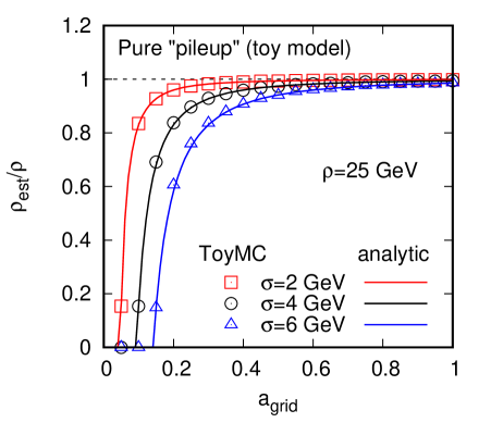
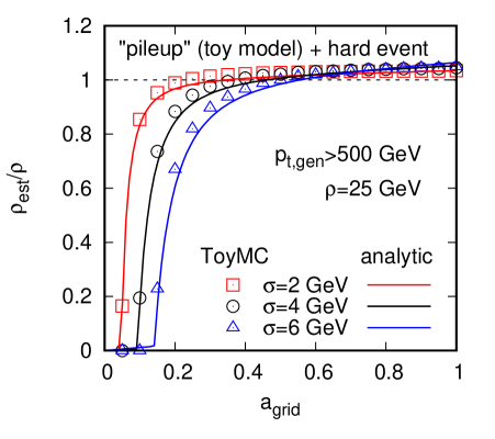
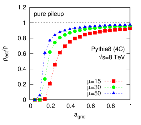
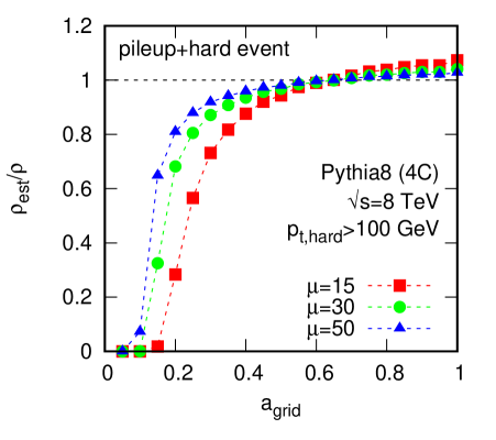
In order to cross-check our calculations, we implemented the toy pileup model in a Monte-Carlo event generator and compared results of numerical simulations to our analytic expectations.

Figure 5.15 shows the comparison for pure-pileup events on the left, and, on the right, for pure-pileup events in which we have embedded dijet events simulated with Pythia 8 with $p_{t,\text{gen}}\geq 500$ GeV (right). In all cases, we have kept the particles up to $|y|=5$ and varied the size of the grid used to estimate $\rho$ between 0.05 and 1 by steps of 0.05. We have fixed $\rho=25$ GeV, a value in the ballpark of what one could expect at the LHC and varied $\sigma$ to probe the scaling of our analytic results. For the analytic curves, we have used $n_{b}=2$, $C_{i}=C_{A}$ and a one-loop running coupling with $n_{f}=5$ and $\Lambda_{\text{QCD}}=100$ MeV. We see that, globally speaking, the analytic expressions do provide a very good qualitative and quantitative description of the features observed in the Monte Carlo simulations.

Finally, we also show on Fig. 5.16 simulations obtained with Pythia 8 for both the hard events and the pileup. Although the quantitative details are different, especially for the transition from $0$ to the region with $\rho_{\rm est}\sim 1$. We know however that this region is sensitive to the details of the pileup model and we should therefore expect that our simplified toy model should at most capture the qualitative features of the full Pythia simulations. The plots on Figs. 5.15 and 5.16 show that it is indeed the case.

Part II Grooming techniques for fat jets

Chapter 6 Main methods

For the second part of this document, we shall switch gear and consider another approach that can be used to mitigate pileup, namely grooming techniques. In this Chapter, we discuss what is meant by grooming and describe the most common techniques that have recently been introduced and used at the LHC. As for the area–median subtraction method discussed in the previous part, we will then carry on with some Monte-Carlo studies, presented in Chapter 7, and finally show that groomers are amenable to some level of analytic understanding in Chapter 8.

Today, grooming techniques are mostly used for specific applications, usually in the context of boosted jets and jet substructure. Compared to the area–median techniques, groomers are not as widely used as generic pileup subtraction tools at the LHC. We shall therefore remain a bit more concise in our presentation than what we have done in the previous part of this document. However, I believe that grooming techniques have the potential to play a crucial role in the development of more advanced pileup mitigation techniques. They are for example an element of the cleansing pileup mitigation technique [11] recently introduced. In the third part of this document, which discusses new pileup mitigation techniques, we shall therefore take an excursion into currently unpublished, preliminary, results trying to use grooming techniques as a generic pileup subtraction tool (see Chapter 10).

6.1 Grooming and tagging fat jets

Let us put aside for a moment the “standard” use of jets at the LHC with relatively small jet radii and work with jets defined with larger $R$, in the range 0.8-1.5. These fat jets are severely affected by pileup and even without any pileup, are still substantially affected by the Underlying Event. One therefore often tries to exclude from the jet a fraction of its constituents which is deemed to contribute essentially to pileup or the UE. For example, one tends to remove soft contamination away from the jet centre, a region indeed expected to be dominated by UE or pileup. This is typically what groomers do: given an input jet, they clean it from soft and large angle radiation and return a groomed jet.

To give a slightly more concrete perspective to this discussion, let us illustrate our arguments with the specific example of filtering. It works as follows: given a jet, one re-clusters its constituents into subjets (with a smaller radius) and keeps only a (pre-decided) fixed number of the hardest subjets (i.e. with the largest $p_{t}$). The union of the subjets that have been kept is the filtered jet. This filtered jet is therefore made of a subset of the original jet’s constituents. Over a bit less than a decade, many grooming techniques have been introduced and we shall briefly review them in the next Section.

We should notice that there is an overlap between the grooming techniques and boosted objects tagging. In a nutshell, the latter refers to the fact that massive objects ($W/Z/H$ bosons or top quarks), when produced with a $p_{t}$ much larger than their mass and when decaying into hadrons, will be reconstructed as single jets. To separate these boosted fat jets, originating from the hadronic decay of a massive object, from the large QCD background, one also exploits the internal properties of jets, i.e. jet substructure. Such techniques are often referred to as taggers.

Taggers and groomers share many similarities, going beyond the simple observation that they are both used on fat jets. Physically, one approach to tag boosted jets is to rely on the fact that massive objects share their $p_{t}$ across their decay products more symmetrically than QCD jets which tend to be dominated by soft radiation. In essence, this approach of finding hard prongs inside a jet bears resemblance to eliminating soft contamination from the Underlying Event or pileup. Hence taggers bear resemblance with groomers. In practice, many tools introduced as groomers can be used as taggers and vice versa. Furthermore, combinations of the two are not uncommon, c.f. the use of filtering after applying a mass-drop tagger in [79].

In my opinion (see also the discussion in [135]), the main difference between a tagger and a groomer lies in what we expect it to do: when we use a tagger, we understand that we want to identify multiple hard prongs in a fat jet with the ultimate goal to maximise signal-to-background efficiency in boosted objects searches; when we use a groomer, we mean that we want to eliminate soft contamination and improve the resolution on the jet kinematics and properties. In other words, a tagger either succeeds or fails, typically according to whether or not it finds hard substructure in the jet, while a groomer always returns a (groomed) jet.

An additional point which is worth keeping in mind in the context of pileup mitigation is that taggers and groomers can be seen as acting on different physical scales (although, in a practical context, the separation may not be as clear): improving the resolution on a jet, the work of groomers, is expected to be done by imposing cuts around the soft UE/pileup scale, while, for taggers, identifying hard prongs in a jet is likely to involve cuts at the perturbative scale(s) of the jet. In the end, this is an area of jet substructure which is still in full development and we can hope for exciting improvements in the next years.

Let us now come back to our original purpose of mitigating pileup. One should understand that grooming technique adopt a different approach to pileup mitigation than the area–median subtraction method used so far. The main conceptual difference is that “standard” pileup subtraction techniques like the area–median method try to correct the jet contaminated by soft radiation back to a jet as it was without that contamination, while grooming techniques would most often affect the hard jets event in the absence of pileup.

This can be understood in the context of our qualitative discussion of pileup effects in Section 2.1. The main goal of the area–median subtraction method is to eliminate the shift due to pileup independently of the hard process one is considering. This means, eliminate, on average, the $\rho A_{\rm jet}$ contamination from the jet. In doing so, the smearing effects are reduced to $\sigma\sqrt{A_{\rm jet}}$. Grooming techniques, on the other hand, target an improvement in $p_{t}$ (or mass) resolution of the jet, i.e. want to reduce as much as possible the $\sigma\sqrt{A_{\rm jet}}$ without guaranteeing an unbiased average contamination. By excluding soft parts of the jet, grooming typically reduces its area from $A_{\rm jet}$ to, say, $A_{\rm groomed}<A_{\rm jet}$. This is not bias-free since it comes at the expense of removing some of the constituents of the original hard jet (a negative bias) and leaving a positive $\rho A_{\rm groomed}$ contribution from pileup. However, it significantly lowers the resolution degradation by reducing it to $\sigma\sqrt{A_{\rm groomed}}$. Adjusting the free parameters of the groomer we could try to minimise the bias while keeping the resolution improvements but this has no guarantee to work on a wide range of applications and contexts.

Both approaches have their advantage. For a broad and robust applications of pileup mitigation to jets with not-so-large $R$, it is crucial to control the average bias and this is what the area–median subtraction method is good at. On the other hand, if one considers a search based on fat jets, appropriate grooming techniques are perfectly suited to obtain a narrow signal peak on a reduced QCD background. Note that, in this case, we also wish to supplement the groomer with area–median subtraction in order to also correct for the positive bias due to $\rho A_{\rm groomed}$ and further improve the resolution when averaging over the full jet sample.

Before digging into the grooming techniques themselves, it is interesting to illustrate some of the arguments above with a concrete example. Let us consider the measurement of the mass of boosted tops reconstructed using fat jets. The area–median subtraction alone would, on average reconstruct the correct average jet mass for both top quarks and pure-QCD jets, with a potentially large smearing due to pileup fluctuations (and the UE). A grooming technique, like filtering briefly introduced above where we would keep the 3 or 4 hardest subjets, would have a different behaviour. For signal jets coming from the hadronic decay of top quarks, one would keep the main structure of the 3-prong decays and hence reconstruct a mass with little average bias, and, at the same time, benefit from the grooming to obtain a good resolution on the mass i.e. a narrower mass peak than without filtering. For standard QCD jets, where most often the mass comes from soft radiation at larger angles, grooming would strongly reduce their mass, already at the perturbative level. This can be a large bias which, in the case of our search for top quarks, plays in our favour since it further suppresses the QCD jet background. Combining grooming and area–median subtraction would further improve the top signal and further reduce the QCD background. We shall see this explicitly in Chapter 7.

6.2 Mass-drop, filtering, trimming, pruning, soft drop

Here, we briefly introduce the main grooming techniques that have been used over the last decade. Some were initially introduced either as taggers, or as both taggers and groomers, but at the end of the day, they all eliminate soft and large-angle radiation and, in that sense, can be seen as groomers.

Filtering.

Given a fat jet, filtering [79] re-clusters its constituents with the Cambridge–Aachen algorithm with a small radius $R_{\rm filt}$. It then only keeps the $n_{\rm filt}$ hardest subjets (in terms of their $p_{t}$). The filtered jet is the union of the subjets that have been kept. This has two adjustable parameters: $R_{\rm filt}$ and $n_{\rm filt}$. It is typically used to reduce soft contamination in situations where we have a prior knowledge of the number of hard prongs in a jet. For a jet with $n_{\rm prong}$ hard prongs — $n_{\rm prong}=2$ for a $W/Z/H$ bosons and $n_{\rm prong}=3$ for a top — we would typically use $n_{\rm filt}=n_{\rm prong}+1$ which would also keep the (perturbative) radiation of an extra gluon. Filtering is implemented directly in FastJet where it is available as the Filter tool (using SelectorNHardest for the selection criterion).

Trimming.

Trimming [136] shares some similarities with filtering. It also starts with re-clustering the jet with a smaller radius, $R_{\rm trim}$, using either the $k_{t}$ or the Cambridge/Aachen algorithm. It then keeps all the subjets with a transverse momentum larger than a fraction $f_{\rm trim}$ of the initial jet transverse momentum. On top of the choice of algorithm, this also has two parameters: $R_{\rm trim}$ and $f_{\rm trim}$. It is often used as a generic groomer and tagger in boosted-jet studies. Trimming can be obtained from the Filter class in FastJet (using SelectorPtFractionMin for the selection criterion).

Pruning.

Pruning [137] is similar in spirit to trimming except that it adopts a bottom-up approach (with trimming seen as a top-down approach). Given a jet, pruning reclusters its constituents using a user-specified jet definition (based on pairwise recombinations) with the additional constraint that at each step of the clustering, objects $i$ and $j$ are only recombined if they satisfy at least one of these two criteria: (i) the geometric distance $\Delta R_{ij}=\sqrt{\Delta y_{ij}^{2}+\Delta\phi_{ij}^{2}}$ is smaller than $R_{\rm prune}=f_{\rm prune}\times 2m_{\rm jet}/p_{t,\rm jet}$, with $p_{t,\rm jet}$ and $m_{\rm jet}$ the original jet transverse momentum and jet mass, (ii) the splitting between $i$ and $j$ is sufficiently symmetric, i.e. ${\rm min}(p_{t,i},p_{t,j})\geq z_{\rm prune}p_{t,(i+j)}$. If none of these criteria are met, only the hardest of $i$ and $j$ (in terms of their $p_{t}$) is kept and the other is rejected. On top of the jet definition used for the re-clustering, which is usually taken to be either $k_{t}$ or Cambridge/Aachen with a radius much larger than the one of original jet, this has two parameters: $f_{\rm prune}$ and $z_{\rm prune}$. $z_{\rm prune}$ plays the same role as $f_{\rm trim}$ for trimming and $f_{\rm prune}$ plays a role similar to $R_{\rm trim}$. Note however that the $R_{\rm prune}$ is defined dynamically with the jet kinematics, compared to $R_{\rm trim}$ which is kept fixed. This can have important consequences both analytically and phenomenologically. Pruning can also be considered as a general-purpose groomer and tagger and is often used in situations similar to trimming. It is available in FastJet as the Pruner class.

$I$ and $Y$-Pruning.

When pruning a jet, there might be situations where a soft emission at large angle dominates the mass of the jet but gets pruned away because it does not satisfy the symmetry condition. The mass of the pruned jet is then determined by radiation at smaller angle, typically within the pruning radius. This situation where the jet mass and the pruning radius are determined by different emissions within the jet would result in a jet with a single prong and are therefore called I-Pruning. For these situations, the pruning radius has no relation to the hard substructure of the jet. More precisely, I-Pruning is defined [135] as the subclass of pruned jets for which, during the sequential clustering, there was never a recombination with $\Delta R_{ij}>R_{\rm prune}$ and ${\rm min}(p_{t,i},p_{t,j})>z_{\rm prune}p_{t,(i+j)}$. The other situation, i.e. a pruned jet for which there was at least one recombination for which $\Delta R_{ij}>R_{\rm prune}$ and ${\rm min}(p_{t,i},p_{t,j})>z_{\rm prune}p_{t,(i+j)}$, corresponds to a genuine two-prong structure and is called Y-Pruning. This distinction between I- and Y-Pruning is mostly relevant for boosted jet tagging. However, it has been shown to have an impact on the analytical behaviour of Pruning, with Y-Pruning being under better control and than I-Pruning, the latter adding quite a lot of complexity to the calculation. If one wishes to reach some level of analytic control over groomed jets, Y-Pruning appears as a more natural choice than Pruning which also includes the I-Pruning class.

Mass-drop.

Originally proposed [79] as a tool to isolate boosted Higgs bosons, decaying to $b\bar{b}$ pairs, from the QCD background, the mass-drop tagger assumes one works with a fat jet clustered with the Cambridge/Aachen algorithm — if it is not the case, one is always at liberty to re-cluster the jet. One then iteratively undoes the last step of the clustering $p_{i+j}\to p_{i}+p_{j}$ until both the following criteria are met: (i) there is a “mass drop” i.e. ${\rm max}(m_{i}.m_{j})<\mu_{\rm cut}m_{i+j}$, (ii) the splitting is sufficiently symmetric i.e. ${\rm min}(p_{t,i}^{2},p_{t,j}^{2})\Delta R_{ij}^{2}>y_{\rm cut}m_{j}^{2}$. When both criteria are met, we keep “$i+j$” as the result of the mass-drop tagger, otherwise the procedure is repeated iteratively keeping only the most massive of $i$ and $j$. If the procedure fails to find two subjets satisfying the conditions, i.e. end up recursing until it reaches a single constituent which cannot be further de-clustered, it is considered as having failed and returns an empty jet. The mass-drop tagger has two parameters: $\mu_{\rm cut}$, the mass-drop parameter itself, and $y_{\rm cut}$, the symmetry cut. The two conditions imposed by the mass-drop tagger make full sense in the physical situation where we want to tag the decay of 2-pronged boosted objects: the symmetry cut requires that one indeed finds two hard prongs and the mass-drop condition imposes that one goes from a massive boson jet to two jets originated from massless QCD partons. Although it was originally introduced as a tagger, the mass-drop tagger also acts as a groomer since, via the Cambridge/Aachen declustering, it would iteratively remove the soft radiation at the outskirts of the jet, hence limiting the pileup/UE contamination. This is available as the MassDropTagger tool in FastJet.

Modified Mass-drop (mMDT).

It has been shown recently [135] that substructure tools can be understood analytically. When trying to understand the behaviour of the mass-drop tagger on QCD jets, it was realised that the fact that the iterative de-clustering was following the most massive of the two branches could lead to pathological situations. It was therefore suggested to adapt the procedure so that it instead follows the hardest branch (in terms of $p_{t}$). This modification has the advantage that it makes the analytical calculation much easier and more robust without affecting the performance of the method (even improving it slightly). The same study also added two more minor modifications. First, it was realised that the symmetry condition could be replaced by ${\rm min}(p_{t,i},p_{t,j})>z_{\rm cut}(p_{t,i}+p_{t,j})$ and that the latter would have a slightly reduced sensitivity to non-perturbative corrections. Second, perturbatively, the mass-drop condition would only enter as a subleading correction (in the strong coupling constant $\alpha_{s}$) compared to the symmetry condition and so could usually be ignored. The ModifiedMassDropTagger is available as part of the RecursiveTools contribution in fjcontrib. By default, it uses a $z_{\rm cut}$ symmetry condition, does not impose a mass-drop condition and follows the highest-$p_{t}$ branch, but variants are allowed in the code.

Soft Drop.

Soft Drop [39] can be seen a generalisation of the modified Mass-drop tagger. It also proceeds by iteratively de-clustering a jet obtained — either directly or re-clustered — with the Cambridge/Aachen algorithm until the Soft Drop condition is met. If we decluster $p_{i+j}$ into $p_{i}$ and $p_{j}$, we stop the de-clustering when

$$\frac{{\rm min}(p_{t,i},p_{t,j})}{p_{t,i}+p_{t,j}}>z_{\text{cut}}\left(\frac{\Delta R_{ij}}{R}\right)^{\beta},$$ (6.1)

with $R$ the jet radius. In the limit $\beta\to 0$, this condition reduces to the mMDT. Hence, Soft Drop can be seen as an extension of the mMDT with the extra parameter $\beta$ allowing for more freedom in constraining the phasespace. Soft Drop has two parameters. The $z_{\text{cut}}$ parameter plays the same role as in the (m)MDT of keeping the hard structure and exclude soft emissions, starting from large angles due to the Cambridge/Aachen de-clustering. The $\beta$ parameter controls how aggressive the groomer is. It goes from no grooming at all for $\beta\to\infty$ to a quite aggressive grooming for $\beta=0$ (mMDT) and carries on with a 2-prong tagging region for $\beta\leq 0$. Used as a groomer, we believe that values of $\beta$ in the range between 1 and 2 are appropriate as they retain some of the large-angle structure of the jet, although larger values could also be used. It is also interesting to realise that, for $\beta=2$, the Soft Drop condition imposes a momentum cut proportional to the square of the angular separation of the two subjets, i.e. proportional to the area of the subjets. One might therefore expect that the choice $\beta=2$ plays a special role when it comes to discussing pileup effects. For example, for $\beta=2$, one could expect the pileup contamination to correspond to a shift in $z_{\rm cut}$. In practice Soft Drop is made available as a SoftDrop class in the RecursiveTools contribution to fjcontrib, where, similarly to the mMDT, it also offers the option to impose an additional mass-drop condition.

Recursive Soft Drop.

One of the potential issues with mMDT and Soft Drop regarding their ability to groom pileup away is that the declustering procedure stops once the condition (6.1) has been met, leaving the jet unchanged at smaller angular sizes. Recursive Soft Drop [138] instead iterates the declustering procedure, either until a fixed number $N+1$ of hard prongs have been found, or until the subjets can no longer be declustered. As a consequence, the grooming is carried on to smaller angular scales and one can expect that the resulting jets have a smaller sensitivity to pileup. For simplicity, we will only consider Soft Drop in this report and refer the reader to Ref. [138] for pileup-mitigation studies with Recursive Soft Drop.

Combination with area–median subtraction.

As discussed earlier, area–median subtraction and groomers target different aspects of pileup mitigation. In many cases it is however possible to combine both approaches in order to benefit both from the correction of the bias implemented in the area–median subtraction and the resolution improvements brought by grooming. We briefly comment on how this can be achieved for the various grooming procedures defined above.

• For the case of filtering and trimming, the idea is to use the area–median subtraction to correct the momentum of the subjets before selecting which ones have to be kept. In the end, the groomed jet would be the union of the subtracted subjets that have been kept. Note that in the case of trimming there is an ambiguity as to whether the condition on the (subtracted) subjet $p_{t}$ uses the subtracted full jet as a reference or the unsubtracted jet. Both options are acceptable and have their respective advantage. Basically, the former tends to be more aggressive than the latter. Depending on the application and the choice of parameters, both options show little practical difference. In terms of the implementation, the combination of filtering/trimming with area–median subtraction can be straightforwardly done by passing a Subtractor to the Filter object. For trimming, it is the end-user’s responsibility to decide whether to pass a subtracted or an unsubtracted jet.

• For pruning, we could also decide, at least on paper, to apply an area–median subtraction at each step of the clustering and impose the pruning criteria on the subtracted jets. This has not yet been implemented in practice. This is due to a purely technical reason: jet areas in FastJet are assigned to the jets a posteriori, hence are not available when one would need them to veto or not a recombination during the re-clustering.

• For the case of the (modified) Mass-drop Tagger and Soft Drop, it is again sufficient to apply the kinematic conditions on subtracted jets. The groomed jet at the end of the procedure would then be the union of the two subtracted subjets found by the iterative de-clustering. In practice, a Subtractor can be passed to both the ModifiedMassDropTagger and to the SoftDrop classes. Note that by default, the original jet is assumed to be unsubtracted and is subtracted internally. Note that the MassDropTagger class in FastJet has no support for internal subtraction so the ModifiedMassDropTagger should be preferred, knowing that the latter could, if needed, be parametrised so as to reproduce the behaviour of the former.

Further discussion, similarities and differences.

Before carrying on with some Monte-Carlo studies of groomers and an example of their analytic properties, there are still a few generic remarks that we find of generic use.

• all the groomers introduced above cut soft particles (or subjets) at large angles. This is either achieved explicitly by removing soft subjets (which are automatically away from the hard subjets by, at least, the subjet radius), or, when using de-clustering, relying on the specific choice of the Cambridge/Aachen jet algorithm, which reflects an angular ordering and therefore throws away soft radiation at large angles until some hard structure is met.

• Since they all implement mainly the same physical ideas, the physical behaviour of all these tools share many similarities, something that can be seen both in Monte Carlo studies and analytic calculations.

• At some point, when the jet boost is increased, important differences between the various groomers start to appear. For example, the fact that the Mass Drop tagger can recurse all the way to arbitrary small opening angle, compared to trimming which has a built-in subjet radius, or to Pruning which has a dynamical minimum angular scale, translates into different behaviour of these three tools. These can sometimes be seen in Monte-Carlo simulations but are best understood when assessing the analytic properties of the groomers.

• Soft Drop differs from the other groomers in that the symmetry cut is angle-dependent. In the end, I believe that this gives Soft Drop some extra flexibility which could prove useful in a broad range of applications. It makes Soft Drop a powerful groomer with nice analytic properties (see also next Chapters).

• In terms of the contamination from pileup (or the UE) at an angular scale $\Delta R$, one would expect an average $p_{t}$ shift of order $\rho\,\pi\Delta R^{2}$. To some extent, this is reminiscent of Soft Drop with $\beta=2$ where the condition would read $z>z_{\text{cut}}(\Delta R/R)^{2}$, suggesting $z_{\text{cut}}\gtrsim A_{\rm jet}\rho/p_{t,\rm jet}$.

Chapter 7 Monte-Carlo studies

So far, most of the practical applications of grooming techniques have concentrated on boosted jets studies. We shall therefore investigate here the performance of grooming as a tool to mitigate pileup effects on boosted jets. This is mostly based on a study that we initially conducted in the context of the proceedings of the Boost 2012 workshop [38], although the new version presented here has been updated to include a broader set of groomers, especially more modern ones. We will come back to grooming techniques as a way to mitigate pileup from generic jets in Chapter 10.

Compared to Ref. [38], this study includes more recent groomers like the modified Mass Drop Tagger and Soft Drop. Similar to the initial study, the events are obtained by combining the hard (signal) events embedded in a series of minimum-bias events to simulate pileup. We consider collisions at a centre-of-mass energy of 13 TeV. Minimum-bias events are generated with the Pythia 8 Monte Carlo (MC) generator [89, 90, 91, 55], with its 4C tune [56]. We considered different pileup conditions, Poisson distributed with $\mu=\{30,60,100,140\}$. This set of choices covers several situations of interest ranging from typical pileup conditions for Run I and II of the LHC up to the exploration of future high intensity scenarii at the LHC.

We have selected two example signals for the Monte Carlo simulation studies presented in this Section. The first is the decay of a possible heavy $Z^{\prime}$ boson with a chosen $M_{Z^{\prime}}=1.5$ TeV to a (boosted) top quark pair, as included in the proceedings of the Boost 2012 workshop. The top and anti-top quarks then decay fully hadronically ($t\to Wb\to jjb$). The second also consists of a $Z^{\prime}$ boson with $M_{Z^{\prime}}=1.5$ TeV, now decaying into $WW$ with both $W$ decaying hadronically. These two samples are meant as sources of 3-pronged and 2-pronged jets, respectively. The signal samples were also generated using Pythia 8 with tune 4C.

The analysis uses the tools either directly available in the FastJet package or in fjcontrib for the jet finding and the jet substructure analysis. The initial jet finding is done with the anti-$k_{t}$ algorithm with $R=1$, to ensure that most of the final state $W$ and top-quark decays can be collected into one jet. For the latter, this corresponds to top-quarks generated with $p_{t}\gtrsim 400$ GeV.

In practice, we will apply several grooming procedures, listed in the next Section, to the original anti-$k_{t}$ jets. For the studies presented in this report we require that the jet $p_{t}$ before grooming and pileup subtraction is larger than 100 GeV. We keep jets with $|y|<3$. We only consider the two hardest $p_{t}$ jets in the event. We further require that the rapidity difference between the two jets $|y_{1}-y_{2}|$ is less than one.

7.1 Jet grooming configurations

Several jet grooming techniques, in use at the LHC, are included in our study (see Chapter 6 for a more complete description):

Trimming. In this study, we used the $k_{t}$ algorithm for the reclustering, with $R_{\mathrm{trim}}=0.2$, and we used $f_{\text{trim}}=0.03$.

Filtering. Here, we reclustered the jets with the Cambridge-Aachen algorithm with $R_{\mathrm{filt}}=0.2$, and kept the $n_{\mathrm{filt}}$ hardest subjets. $n_{\mathrm{filt}}$ has been varied according to the process under consideration and we found good results using $n_{\mathrm{filt}}=2$ for the $Z^{\prime}\to WW$ process and $n_{\mathrm{filt}}=4$ for the $Z^{\prime}\to t\bar{t}$ case.

modified Mass Drop (mMDT) and Soft Drop (SD). We have fixed $z_{\mathrm{cut}}=0.1$ and studied $\beta=0$ (mMDT), $1$ and $2$ (SD). Following the original prescription of [79], we have optionally applied to the result of the mMDT/SD procedure, an extra step of filtering, using $R_{\rm filt}={\rm max}(R_{\rm SD},0.2)$ with $R_{\rm SD}$ the distance between the two prongs found by the mMDT/SD, and $n_{\rm filt}$ as for the plain filtering case described above. In a nutshell, once the mMDT/SD procedure has found a 2-pronged structure, thereby excluding radiation at angles larger than $R_{\rm SD}$, this extra filtering step further cleans the contamination at smaller angles.

A specific point we want to study is the interplay between jet grooming and area-based pileup correction. The subtraction is applied directly on the 4-momentum of the jet using the area–median approach, Eq. (2.30), with the active area of the jet computed using FastJet. We included the $\rho_{m}$ term which corrects for contamination to the total jet mass due to the mass of the pileup particles. The estimation of $\rho$ and $\rho_{m}$ is performed with FastJet using a grid-based estimate with a grid of cell-size 0.55 extending to $|y|=4$. Corrections for the rapidity dependence of the pileup density $\rho$ are applied using a rapidity rescaling (see Sections 2.4.2 and 3.1). Ghosts are placed up to $y_{\rm max}=4$ and explicit ghosts are enabled, ensuring the availability of the area information to grooming tools. When applying this subtraction procedure, we discard jets with negative transverse momentum or (squared) mass of the jet.

When we apply this background subtraction together with grooming, the subtraction is performed directly on the subjets, before applying any kinematic constraint, i.e. before deciding which subjets should be kept, in the case of trimming and filtering, or before checking if the symmetry criterion is met in the case of mMDT and Soft Drop. This is meant to limit the potential effects of pileup on kinematic tests. Note that in the case of trimming, the unsubtracted jet $p_{t}$ is used as the reference to compute the $p_{t}$ threshold for subjets. It was found that this gives slightly better results than using the subtracted jet.

7.2 Jet substructure performance

(a) raw, ungroomed jets

(b) raw jets with pileup subtraction

(c) trimmed jets

(d) trimmed jet with pileup subtraction

(e) filtered jets

(f) filtered jet with pileup subtraction

Figure 7.1: The impact of $N_{\mathrm{PU}}$ on the jet mass distribution. Top row: the raw jet mass distribution for $Z^{\prime}\to t\bar{t}$ final states with $m_{Z^{\prime}}=$ 1.5 TeV, in the presence of pileup with $\mu=30$, 60, 100, and 140, before (left) and after (right) area–median pileup subtraction. The second and third rows show the same results after trimming (middle row) and filtering (lower row).

(a) jets after mMDT

(b) jets after mMDT+filtering

(c) jets after SoftDrop($\beta=1$)

(d) jets after SoftDrop($\beta=1$)+filtering

(e) jets after SoftDrop($\beta=2$)

(f) jets after SoftDrop($\beta=2$)+filtering

Figure 7.2: Same as Fig. 7.1 now showing the jet mass distribution after applying the modified Mass Drop (top row) or Soft Drop with $\beta=1$ (middle row) or $\beta=2$ (lower row). All distributions are shown after area–median pileup subtraction. Plots on the left column show the results of the initial grooming procedure alone, and plots on the right column show the results with an extra filtering step (see text for details).

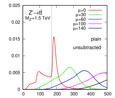
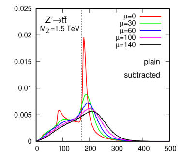
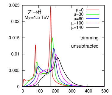
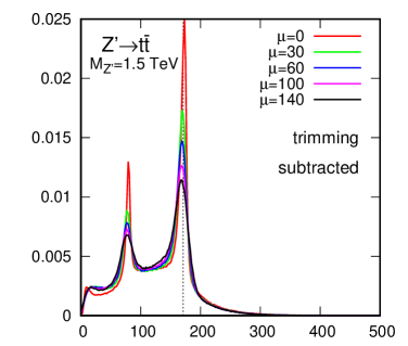
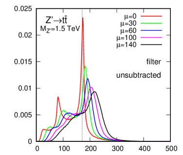
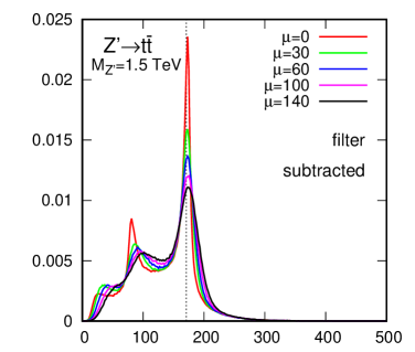
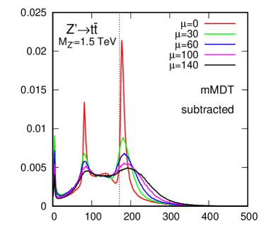
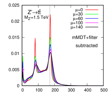
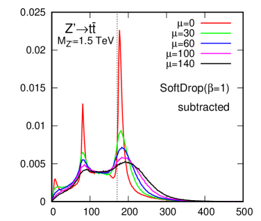
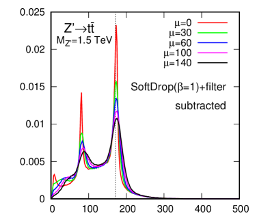
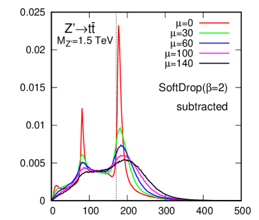
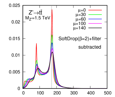
As a first test, we look at the jet mass distribution obtained for out $Z^{\prime}\to t\bar{t}$ event sample. This is plotted in Figs. 7.1 and 7.2. The immediate expectation for the reconstructed jet mass is the top mass, i.e. $m\approx 171$ GeV, and no residual dependence on the pileup activity $\mu$, after the pileup subtraction. The two plots in the upper row of Figure 7.1 show the distributions of the reconstructed jet masses: without pileup subtraction on the left (7.1(a)) and with area–median pileup subtraction on the right (7.1(b)). Concentrating on the sample without any pileup added, we see that a large fraction of the events are reconstructed close to the top mass and about 30% are compatible with the $W$ mass. The effect of pileup on the mass scale and resolution is clearly visible, increasingly shifting the peak towards much larger jet masses and smearing it.

Applying only the pileup subtraction, without applying any grooming to the jets, already improves the mass reconstruction significantly. The pileup shift is mostly removed from the jet mass spectrum, as shown in Fig. 7.1(b) and the position of the mass peak is recovered, independently of $\mu$. With increasing pileup, the mass peak gets more and more smeared, an effect that we have already seen in the first part of this document, due to the fact that the pileup is not perfectly uniform. We have already stressed that these point-to-point fluctuations in an event lead to a smearing by $\pm\sigma\sqrt{A}$ in the subtracted jet $p_{t}$. For very large pileup, this smearing extends all the way to $m=0$ as seen in Fig. 7.1(b) and we lose the clean separation between the $W$ and the top mass peaks.

The effect of the grooming techniques on the reconstructed jet mass distributions is summarised in the remaining plots of Figs. 7.1 and 7.2. For filtering and trimming, Figs. 7.1(c)-(f), we show the mass distributions with and without subtraction, while for the plot of Fig. 7.2 we show the result of the mMDT/SD procedure with and without the extra filtering step. The spectra show that grooming clearly improves the mass reconstruction. Already without applying area–median pileup subtraction, one sees that the peak is much less shifted and smeared than in the ungroomed case. The application of the pileup subtraction in addition to the grooming procedure further improves the mass reconstruction performance, fully correcting for the peak position and further improving the resolution. From Fig. 7.2, we also see that applying filtering on the result of the mMDT/SD grooming further improves the quality of the reconstructed spectrum.

The fact that the combination of grooming and area–median pileup subtraction appears as the optimal combination should not be a surprise. As discussed many times already, pileup has mainly two effects on the jet: a constant shift proportional to $\rho A$ and a smearing effect proportional to $\sigma\sqrt{A}$, with $\sigma$ a measure of the fluctuations of the pileup within an event. In that language, the subtraction corrects for the shift leaving the smearing term untouched. Grooming, on the contrary, since it selects only part of the subjets, acts as if it was reducing the area of the jet. This reduces both the shift and the dispersion. Combining grooming with subtraction thus allows to correct for the shift leftover by grooming and reduce the smearing effects at the same time. All these effects are observed on the plots.

The effect of the filtering step applied after the mMDT/SD grooming can also be understood from fairly simple arguments: the declustering procedure applied by mMDT/SD discards the soft activity at large angles in the jet until two hard prongs are found. This effectively reduces the jet area with the immediate consequence of reducing the shift and smearing of the mass peak. However, this results in a groomed jet with an effective radius dictated by the hard-prong structure of the jet. Say we have a 500 GeV $W$ boson, this corresponds to a grooming radius around $R_{\rm SD}\approx 0.4$ which gives an area $\pi R_{\rm SD}^{2}$ still larger that the typical $2\pi R_{\rm filt,trim}^{2}$ obtained with filtering or trimming. Applying an extra filtering step to the result of the mMDT/SD, as already suggested in the original work [79], would further groom the jet at angular scales smaller than the original grooming radius, further reducing the effective jet area and hence further reducing the peak shift and smearing.

Figure 7.3: Position (leftmost figure) and width (rightmost figure) of the reconstructed jet mass distribution in $Z^{\prime}\to t\bar{t}$ final states (top row) and $WW$ events (bottom row), as a function of the pileup activity $\mu$, for various jet grooming techniques. Area–median pileup subtraction is applied in all cases.

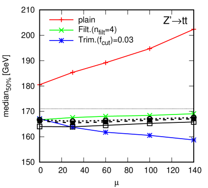
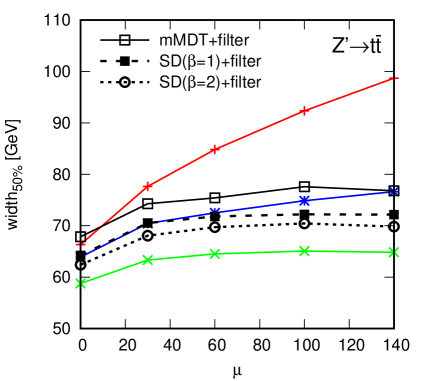
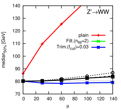
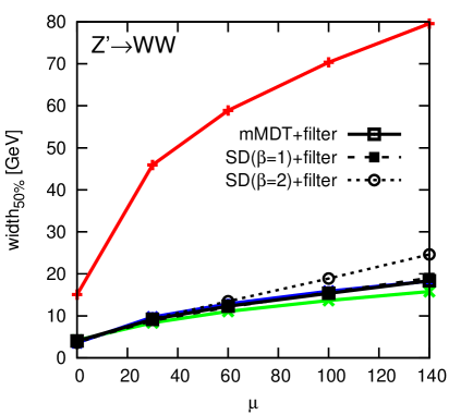
To summarise in a more compact way the above findings and quantify more precisely the performance of the various grooming techniques analysed in this study, we have measured the position and width of the peak in all our different scenarii. We define this by looking, for each individual mass distribution, at the narrowest mass window that contains 50% of the reconstructed jets. We then define the peak position as the median of that window and the peak width as the width of the mass window. The findings from the spectra are quantitatively summarised in Fig. 7.3 for the peak position (left) and width (right), for both the top (top) and the $W$ (bottom) samples. Since we have already seen that the combination of grooming with area–median subtraction was performing better than grooming alone, and that mMDT/SD was working best when supplemented with a filtering step, we focused only on these optimal cases.

We see that all methods succeed at maintaining the jet mass independent of the pileup conditions and around the expected mass value of 171 GeV, although the reconstructed average top mass tends to be slightly underestimated. This works well for all groomers even at large pileup multiplicity, although some differences are observed between the various groomers. All the groomers studied here improve the mass resolution to different degrees, but in any case perform better than pileup subtraction alone, as expected. Combining area-subtraction and filtering yields the least sensitivity to pileup in terms of the peak position and width, especially for the $t\bar{t}$ sample. For the $WW$ sample, all groomers tend to perform similarly. The observed differences are anyway beyond the scope of this study and depend also on the specific choice of parameters for the different groomers.

7.3 Summary

A brief Monte Carlo study of the effect of jet grooming techniques on the jet mass reconstruction in $Z^{\prime}\to t\bar{t}$ and $Z^{\prime}\to WW$ final states has been conducted. Jet trimming, filtering, the modified Mass-Drop tagger and Soft Drop are used by themselves, or in combination with the pileup subtraction using the four-vector area, to reconstruct the single jet mass and evaluate the stability of the mass scale and resolution at pileup levels of 30, 60, 100, and 140 extra $pp$ collisions, in addition to the signal event. We find that for these particular final states all groomers work well for maintaining the mass scale and resolution, provided they are applied together with pileup subtraction so as to benefit both from the average shift correction from subtraction and noise reduction from the grooming. The results are stable up to large pileup multiplicities. In the case of the mMDT/SD procedures, we find useful to supplement them with an extra filtering step as suggested in the original work from Ref. [79].

Finally, note that a more thorough comparison of the performance of these groomers would require varying their parameters. This goes beyond the scope of this study.

Chapter 8 Analytical insight

8.1 Foreword

We have seen that groomers are an efficient way to reduce pileup contamination from fat jets. Another aspect of groomers is that, even in the absence of pileup, they affect the structure of the hard jets in the event. This is usually a desired feature since it implies a reduction of the QCD background compared to the heavy-object signal when tagging boosted objects.

In this chapter we illustrate that the perturbative behaviour of groomers is amenable to an analytic treatment. After the very first results on the MassDrop Tagger, trimming and pruning in Refs. [135, 139], we have shown [39] that an analytic treatment is also possible for SoftDrop. To keep the discussion relatively contained and to avoid departing too much from the main theme of this document, we will just concentrate on a single observable, namely the groomed jet radius after one applies SoftDrop to a boosted jet. We will show that it can be computed in QCD in for boosted objects. This also covers the case of the modified MassDropTagger [135] which can be obtained from the SoftDrop results by taking the limit $\beta\to 0$. We refer directly to [135], [39] and [72] for additional analytic results for substructure techniques.

At first sight, this does not seem directly related to pileup mitigation. However, we believe that an analytic understanding of common tools in the field of jet substructure is crucial-enough that we devote a few pages to that topic. Furthermore, one might ultimately want to use insight from QCD first-principle calculations to develop optimal pileup subtraction techniques, e.g. to control their biases and sensitivities to different dynamical properties of the jet. The analytic control over groomers described in the next few pages can therefore also be seen as a step towards this broader goal. In particular, the groomed jet radius is one observable that is directly related to the residual sensitivity of the groomed jet to pileup. Gaining analytic control over it could be helpful in devising better pileup mitigation techniques.

We will also provide a brief Monte-Carlo study of non-perturbative effects for SoftDropped jets. In practice, it is partially possible to address the question of non-perturbative effects from an analytic perspective. Unfortunately, this work is still too preliminary to deserve a place here, although we can say that the underlying idea follows the non-perturbative calculation done for the modified Mass-Drop Tagger in Ref. [135].

8.2 Groomed Jet Radius

Because the soft drop procedure is defined through declustering a Cambridge/Aachen branching tree, there is a well-defined and IRC-safe meaning to the groomed jet radius. Concretely, the groomed jet radius $R_{g}$ is the angle between the branches that first satisfy the SoftDrop condition (6.1). This is sensible since for a Cambridge/Aachen tree, all subsequent branches are separated by an angle less than $R_{g}$. From a practical perspective, $R_{g}$ is particularly interesting, since the groomed jet area is approximately $\pi R_{g}^{2}$. Thus, $R_{g}$ serves as a proxy for the sensitivity of the groomed jet to possible contamination from pileup.

8.2.1 Analytic calculation

In what follows, we will provide an analytic calculation of the $R_{g}$ distribution valid in the small-angle limit, $R_{g}\ll R\ll 1$, pertinent e.g. for the boosted jet regime, and focus on the leading logarithmic terms.

At this accuracy it is sufficient to assume that the jet is composed of the “leading parton” accompanied by independent soft-and-collinear emissions strongly ordered in angle and energy. Assume we have $n$ such emissions with strongly-ordered angles to the jet axis, $\theta_{1}\gg\theta_{2}\gg\dots\gg\theta_{n}$. We also denote by $z_{1},\dots,z_{n}$ their respective transverse momentum fraction. The grooming radius will be $\theta_{i}$ if emission $i$ is kept by Soft Drop and all previous emissions $1,\dots,i-1$ are groomed away. The grooming radius condition for that set of emissions can thus be written as

$$\delta(R_{g}(\{\theta_{i},z_{i}\})-R_{g})=\sum_{i=1}^{n}\Theta_{i}^{\text{in}}\prod_{j=1}^{i-1}\Theta_{j}^{\text{out}}\delta(\theta_{i}-R_{g})+\prod_{i=1}^{n}\Theta_{i}^{\text{out}}\delta(R_{g}),$$ (8.1)

where $\Theta_{i}^{\text{in}}$ indicates that emission $i$ is kept by Soft Drop while $\Theta_{i}^{\text{out}}$ indicates that it is groomed away. The last term in the above expression corresponds to the situation where all emissions are groomed and where we have decided to set $R_{g}=0$ in this case for simplicity. Recall also that if emission $i$ is kept by grooming, all subsequent emissions at smaller angles will be kept as well.

We then have to sum over any number of such emissions and obtain the following expression for the groomed jet radius

$$\frac{R_{g}}{\sigma}\frac{d\sigma}{dR_{g}}=\lim_{\epsilon\to 0}\sum_{n=0}^{\infty}\prod_{i=0}^{n}\int_{\epsilon}^{R}\frac{d\theta_{i}}{\theta_{i}}\int_{\epsilon}^{1}dz_{i}\,p(z_{i}) \,\frac{\alpha_{s}(z_{i}\theta_{i}p_{t})}{\pi}\>\Theta(\theta_{i}>\theta_{i+1})$$ (8.2)

$$R_{g}\delta(R_{g}(\{\theta_{i},z_{i}\})-R_{g})\>\exp\bigg{[}-\int_{\epsilon}^{R}\frac{d\theta}{\theta}\int_{\epsilon}^{1}dz\,p(z)\,\frac{\alpha_{s}(z\theta p_{t})}{\pi}\bigg{]}.$$

To write (8.2), we have introduced $\epsilon$ to regulate the soft and collinear divergences. The last, exponential, term corresponds to virtual corrections and will cancel the soft and collinear divergences in the end so that one can safely take the limit $\epsilon\to 0$. The argument of the strong coupling is taken as the relative transverse momentum of the emitted gluon w.r.t. the parent parton. Finally, $p(z)$ is the appropriate splitting function different for quark-initiated jets and gluon-initiated jets.

To evaluate (8.2), we first notice that the $\delta(R_{g})$ in (8.1) will vanish in the limit $\epsilon\to 0$. Indeed, if all the emissions are outside of the grooming radius, the sum over real emissions factorises into

$$\sum_{n=0}^{\infty}\prod_{i=0}^{n}\int_{\epsilon}^{R}\frac{d\theta_{i}}{\theta_{i}}\int_{\epsilon}^{1}dz_{i}\,p(z_{i})\,\frac{\alpha_{s}(z_{i}\theta_{i}p_{t})}{\pi}\>\Theta(\theta_{i}>\theta_{i+1})\Theta_{i}^{\text{out}}=\exp\bigg{[}\int_{\epsilon}^{R}\frac{d\theta}{\theta}\int_{\epsilon}^{1}dz\,p(z)\,\frac{\alpha_{s}(z\theta p_{t})}{\pi}\,\Theta^{\text{out}}\bigg{]}.$$ (8.3)

Combined with virtual corrections, this gives

$$\exp\bigg{[}-\int_{\epsilon}^{R}\frac{d\theta}{\theta}\int_{\epsilon}^{1}dz\,p(z)\,\frac{\alpha_{s}(z\theta p_{t})}{\pi}\,\Theta^{\text{in}}\bigg{]}$$ (8.4)

which vanishes in the limit $\varepsilon\to 0$.

Then, for the remaining terms in (8.1), it is helpful to reorganise the emissions where we pull out in front the integration over $\theta_{i}$ such that $\theta_{i}=R_{g}$, and rename it $\theta_{0}$. We then separate the remaining emissions in two groups: those at larger angles for which we have to impose the condition that they are outside the Soft Drop region (see (8.1)), and those at smaller angles which are automatically kept by Soft Drop. The first series can set to have $n$ emissions with momenta and angles $(z_{1},\theta_{1}),\dots,(z_{n},\theta_{n})$ and the second series $\bar{n}$ emissions with momenta and angles $(\bar{z}_{1},\bar{\theta}_{1}),\dots,(\bar{z}_{\bar{n}},\bar{\theta}_{\bar{n}})$, where we have to sum over $n$ and $\bar{n}$. This gives

$$\frac{R_{g}}{\sigma}\frac{d\sigma}{dR_{g}}=\lim_{\epsilon\to 0} \int_{\epsilon}^{R}\frac{d\theta_{0}}{\theta_{0}}\int_{\epsilon}^{1}dz_{0}\,p(z_{0})\,\frac{\alpha_{s}(z_{0}\theta_{0}p_{t})}{\pi}R_{g}\delta(R_{g}(\theta_{0}-R_{g}))\Theta(z_{0}>z_{\text{cut}}(R_{g}/R)^{\beta})$$ (8.5)

$$\sum_{n=0}^{\infty}\frac{1}{n!}\prod_{i=0}^{n}\int_{\theta_{0}}^{R}\frac{d\theta_{i}}{\theta_{i}}\int_{\epsilon}^{1}dz_{i}\,p(z_{i})\,\frac{\alpha_{s}(z_{i}\theta_{i}p_{t})}{\pi}\Theta(z_{i}<z_{\text{cut}}(\theta_{i}/R)^{\beta})$$

$$\sum_{\bar{n}=0}^{\infty}\frac{1}{\bar{n}!}\prod_{j=0}^{n}\int_{\epsilon}^{\theta_{0}}\frac{d\bar{\theta}_{j}}{\bar{\theta}_{j}}\int_{\epsilon}^{1}d\bar{z}_{j}\,p(\bar{z}_{j})\,\frac{\alpha_{s}(\bar{z}_{j}\bar{\theta}_{j}p_{t})}{\pi}\>\exp\bigg{[}-\int_{\epsilon}^{R}\frac{d\theta}{\theta}\int_{\epsilon}^{1}dz\,p(z)\,\frac{\alpha_{s}(z\theta p_{t})}{\pi}\bigg{]}.$$

Once again, the sums over $n$ and $\bar{n}$ lead to exponentials:

$$\sum_{n=0}^{\infty}\frac{1}{n!}\prod_{i=0}^{n}\int_{\theta_{0}}^{R}\frac{d\theta_{i}}{\theta_{i}}\int_{\epsilon}^{1}dz_{i}\,p(z_{i})\, \frac{\alpha_{s}(z_{i}\theta_{i}p_{t})}{\pi}\Theta(z_{i}<z_{\text{cut}}(R_{g}/R)^{\beta})$$ (8.6)

$$=\exp\bigg{[}-\int_{\theta_{0}}^{R}\frac{d\theta}{\theta}\int_{\epsilon}^{1}dz\,p(z)\,\frac{\alpha_{s}(z\theta p_{t})}{\pi}\,\Theta(z<z_{\text{cut}}(\theta/R)^{\beta})\bigg{]},$$

and

$$\sum_{\bar{n}=0}^{\infty}\frac{1}{\bar{n}!}\prod_{j=0}^{n}\int_{\epsilon}^{\theta_{0}}\frac{d\bar{\theta}_{j}}{\bar{\theta}_{j}}\int_{\epsilon}^{1}d\bar{z}_{j}\,p(\bar{z}_{j})\,\frac{\alpha_{s}(\bar{z}_{j}\bar{\theta}_{j}p_{t})}{\pi}=\exp\bigg{[}-\int_{\epsilon}^{\theta_{0}}\frac{d\theta}{\theta}\int_{\epsilon}^{1}dz\,p(z)\,\frac{\alpha_{s}(z\theta p_{t})}{\pi}\bigg{]}.$$ (8.7)

These exponentials combine with the virtual corrections in particular to cancel the divergence at $\epsilon\to 0$ as expected and give, after integration over $\theta_{0}$

$$\frac{R_{g}}{\sigma}\frac{d\sigma}{dR_{g}}=\int_{0}^{1}dz_{0}\,p(z_{0})\,\frac{\alpha_{s}(z_{0}R_{g}p_{t})}{\pi}\Theta\Big{(}z_{0}>z_{\text{cut}}\frac{R_{g}^{\beta}}{R^{\beta}}\Big{)}\exp\bigg{[}-\int_{R_{g}}^{R}\frac{d\theta}{\theta}\int_{0}^{1}dz\,p(z)\,\frac{\alpha_{s}(z\theta p_{t})}{\pi}\,\Theta\Big{(}z>z_{\text{cut}}\frac{\theta^{\beta}}{R^{\beta}}\Big{)}\bigg{]}.$$ (8.8)

The above expression can easily be evaluated for quark and gluon jets, using a 1-loop running-coupling approximation for $\alpha_{s}$. This is what we have done for the comparison to Monte-Carlo simulations presented in the next Section. It is nevertheless illustrative to consider the fixed-coupling approximation which gives (up to subleading power corrections)

$$\int_{0}^{1}dz_{0}\,p(z_{0})\,\frac{\alpha_{s}}{\pi} =\frac{\alpha_{s}C_{R}}{\pi}\bigg{[}\log\Big{(}\frac{1}{z_{\text{cut}}R_{g}^{\beta}}\Big{)}+B_{i}\bigg{]},$$ (8.9)

$$\int_{R_{g}}^{R}\frac{d\theta}{\theta}\int_{0}^{1}dz\,p(z)\,\frac{\alpha_{s}}{\pi}\,\Theta\Big{(}z>z_{\text{cut}}\frac{\theta^{\beta}}{R^{\beta}}\Big{)} =\frac{\alpha_{s}C_{R}}{\pi}\bigg{[}\log\Big{(}\frac{R^{\beta/2}}{z_{\text{cut}}R_{g}^{\beta/2}}\Big{)}+B_{i}\bigg{]}\log\Big{(}\frac{R}{R_{g}}\Big{)},$$ (8.10)

with $C_{R}=C_{F}$ and $B_{i}=-3/4$ for quark-initiated jets, and $C_{R}=C_{A}$ and $B_{i}=(11C_{A}-4n_{f}T_{R})/(12C_{A})$ for gluon-initiated jets. This corresponds to a double-logarithmic suppression in $R/R_{g}$ which becomes single-logarithmic for $\beta=0$.

Figure 8.1: Phase space for emissions relevant for groomed jet radius $R_{g}$ in the $(\log\frac{1}{z},\log\frac{R}{\theta})$ plane. The region groomed away by Soft Drop is grey and the first emission satisfying the soft drop criteria is illustrated by the red dot which can be anywhere on the thick blue line. The forbidden emission region (the Sudakov exponent) is shaded in pink.

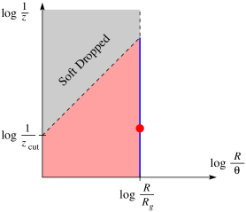
It is also helpful to give a physical interpretation of (8.8). This is illustrated in Fig. 8.1 where we represent the phase-space available for emission in the $(\log\frac{1}{z},\log\frac{R}{\theta})$ plane. If one wants a given grooming radius $R_{g}$, we need an emission at an angle $R_{g}$ passing the Soft Drop condition. This corresponds to the red dot in the Figure which can lie anywhere on the thick blue line. It leads to the prefactor in (8.8) where the integration over $z_{0}$ corresponds to the red dot spanning the blue line. We then need to guarantee that the Soft Drop procedure does not stop at a larger radius. We should therefore veto all real emissions at larger angles and that would pass the Soft Drop criterion. This is represented by the pink shaded area in the figure and to the Sudakov suppression factor in Eq. (8.8). Since real emissions are vetoed in that region, only virtual corrections remain. In all the rest of the phasespace, real emissions are allowed and cancel against virtual corrections.

On a more technical basis, it is worth noting that the groomed jet radius $R_{g}$ is also simple in terms of multiple-emission corrections. Indeed, once one emission satisfies the soft drop criteria, the jet radius is set, so multiple emissions do not contribute to this observable. We can also verify that non-global contributions are suppressed by $R_{g}$ for $\beta<\infty$. For these reasons, we believe that the expression in Eq. (8.8) is fully accurate to single-logarithmic level.

8.2.2 Comparison to Monte Carlo

Figure 8.2: Comparison of the jet radius $R_{g}$ distribution extracted from Pythia 8 (left, solid) and inferred from the active area in Pythia 8 using $R_{\text{eff}}=\sqrt{A_{\text{active}}/\pi\xi}$ (left, dashed), and computed to modified leading logarithmic accuracy (right). The original jet radius is set to be $R=1$ and the jets have an ungroomed energy of $3$ TeV. The Soft Drop parameter is $z_{\text{cut}}=0.1$, while $\beta$ is varied.

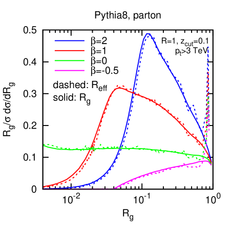
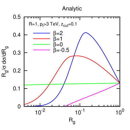
There are two different ways one can define the groomed jet radius in Monte Carlo. The first method is to simply measure the $R_{g}$ value of the Cambridge/Aachen branching that satisfies the Soft Drop condition. A second approach, more directly connected with pileup mitigation, is to determine the effective radius of the groomed jet from its active area (see Section 2.3.3). An effective jet radius $R_{\text{eff}}$ can then be defined from the groomed jet active area using:

$$R_{\text{eff}}\equiv\left(\frac{A_{\text{active}}}{\pi\xi}\right)^{1/2}\ ,$$ (8.11)

where $A_{\text{active}}$ is the active jet area, and $\xi\simeq(1.16)^{2}$ accounts for the fact that a typical Cambridge/Aachen jet of radius $R$ has an average active area $\xi\pi R^{2}$.

To compare $R_{g}$ and $R_{\text{eff}}$ and to validate our analytic calculation (8.8), we have generated with Pythia 8 (v8.176) 14 TeV $qq\to qq$ events and selected anti-$k_{t}(R=1)$ jets with $p_{t}\geq 3$ TeV. We have applied the Soft Drop procedure with $z_{\text{cut}}=0.1$ and different values of $\beta$ and computed $R_{g}$ and $R_{\text{eff}}$. To obtain $R_{\text{eff}}$ in practice, we have computed the groomed jet area using active areas as implemented in FastJet (v3), and we used a ghost area of 0.0005 and 10 repetitions in order to reach sufficiently small values of $R_{\rm eff}$.

The resulting distributions are plotted in the left plot of Fig. 8.2. With the $\xi$ offset factor, the two techniques give remarkably similar results, giving strong evidence that the groomed jet radius $R_{g}$ is an effective measure of pileup sensitivity. The main difference is the spike at $R_{\rm eff}=1/\sqrt{\xi}$, corresponding to cases where the first Cambridge/Aachen branching already satisfies the soft drop condition, yet typically with $R_{g}<1$. The nice reduction of the jet area even with mild grooming (e.g.  $\beta=2$) suggests that Soft Drop should work well for pileup mitigation.

In the right plot of Fig. 8.2, we show the distribution obtained from our analytic calculation, Eq. (8.8). There is good qualitative agreement with Pythia for a range of angular exponents $\beta$, suggesting that our modified leading-logarithmic calculation for $R_{g}$ captures much of the relevant physics effects present in the Monte Carlo simulation and that analytic calculations can be helpful in understanding how grooming techniques mitigate pileup.

Note that when increasing the jet $p_{t}$, one would effectively reduce the coupling $\alpha_{s}(p_{t}R)$ arising naturally from (8.8). Both the pre-factor and Sudakov exponent would then be reduced, shifting the peak in the $R_{g}$ distribution to smaller values.

8.3 Non-Perturbative Contributions

Figure 8.3: Effect of non-perturbative corrections on $R_{g}$. The left plot shows the ratio between hadron level and parton level predictions obtained with Pythia 8 (without UE). The right plot instead shows the ratio of hadron-level results with and without UE.

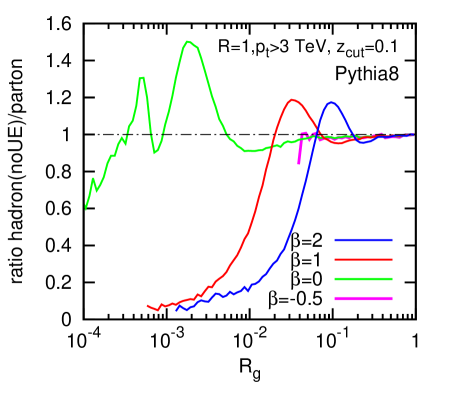
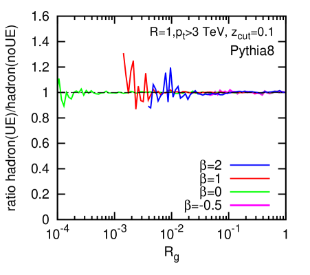
In the above analytic calculations and Monte-Carlo simulations, we only considered the distributions generated at parton level. In this section, we present a brief Monte Carlo study to estimate the impact that non-perturbative effects from hadronisation and UE can have on the groomed jet radius distribution.

In Fig. 8.3, we show the effect of hadronisation (left) and UE (right) on the $R_{g}$ distribution for different values of $\beta$. In the case of hadronisation, we plot the ratio between the hadronic and partonic distributions obtained from Pythia 8. In the case of UE, we plot the ratio between the distributions with and without UE. Apart from including non-perturbative effects, the details of the analysis are the same as for the previous Monte Carlo studies.

The left plot in Fig. 8.3 shows that Soft Drop declustering pushes the onset of hadronisation corrections to smaller values of $R_{g}$ with decreasing $\beta$. As shown in the right plot of Fig. 8.3, Soft Drop has the remarkable ability to reduce the UE contribution to almost zero down to very small values of $R_{g}$.

Part III Towards more efficient techniques

Chapter 9 Challenges beyond the area–median subtraction

9.1 Motivation

Let us put aside the specific case of fat jets and their grooming, and come back to our original task: providing a generic-purpose pileup mitigation technique that can be used for standard jet reconstruction at the LHC. This covers the majority of cases where jets are used at the LHC today. In the same kind of spirit, in most of the analysis where jets are used, the fundamental quantity that we use is the jet transverse momentum. In this last part, we shall therefore focus on pileup mitigation for “standard” jet clustering and mainly consider the most widely used jet characteristic: its transverse momentum. We shall only briefly investigate the case of other jet properties like the jet mass or even other jet shapes, and some applications to boosted jets. One should however keep in mind that even if these jet substructure observables are of growing importance, they usually have to be considered together with grooming techniques for practical applications.

In the first part of this document we have seen that the area–median pileup subtraction technique does a very good job at correcting, event by event, for the transverse momentum shift induced by pileup. A benefit of the event-by-event nature of the subtraction is that it also reduces the associated resolution degradation. The area–median is therefore an efficient pileup-mitigation tool that has proven perfectly adequate for the Run I of the LHC and at least the beginning of Run II, with values of $\mu$ slightly above 40 as of October 2016. However, as the LHC luminosity increases, so will $\mu$, the average number of pileup interactions per bunch crossing. One might expect values of $\mu$ around 60 at maximal luminosity already in Run II, and in perspectives for the High-Luminosity LHC, one quotes values of $\mu$ that can reach the $140{-}200$ range. While the area–median subtraction method would still be efficient at correcting for the average $p_{t}$ shift, with higher pileup multiplicities, the effects of fluctuations would increase substantially. From the 6 GeV observed for 30 pileup interactions in Fig. (3.8), one should expect a resolution smearing of about 7.5 GeV for 60 pileup interactions and more than 10 GeV above 100, in good agreement with a scaling proportional to $\sqrt{{N_{\mathrm{PU}}}}$. This increase should not be too dramatic for very high-$p_{t}$ jets where detector resolution effects dominate over the pileup smearing effects, but become an issue for low-$p_{t}$ jets.

One could simply decide to increase the minimal jet $p_{t}$ threshold. However, the feasibility of key measurements at the LHC — like double-Higgs production, jet vetoes and the study of the properties of the Higgs boson — depend on the experiments’ ability to reconstruct jets down to transverse momenta as low as 20 GeV. This situation is therefore far from ideal and has lead people to think about alternative pileup mitigation techniques.

In what follows, we shall discuss new ideas going along two different main avenues. The first one follows a logic similar to the area–median subtraction technique: it focuses on correcting for the right average pileup contamination but further uses additional information in the event. The typical example here is the case of charged tracks. With current technology, the experiments can associate charged tracks to a vertex of origin and discard those coming from pileup vertices. One is then left with pileup mitigation on the neutral part of the event. Although we do not want to enter into the experimental details, this is a core idea in the Charged-Hadron Subtraction (CHS) method in CMS. In an ideal situation, this would correct exactly for the charged part of pileup. Applying pileup subtraction on the remaining neutral part, e.g. using the area–median subtraction, would mean that, in the end, the resolution degradation is only affected by the neutral fluctuations of pileup. Since about 60% of the energy goes into charged particles, this would automatically reduce the resolution degradation by a factor around $\sqrt{0.4}\approx 0.63$. With this technique, the pileup smearing effects for ${N_{\mathrm{PU}}}=100$ would only be slightly worse than what one sees without using charged-track information at ${N_{\mathrm{PU}}}=30$. We shall discuss at length the use of charged tracks to mitigate pileup in Chapter 11 below, including the adaptation of the area–median method as well as other alternatives.

The second approach is to explicitly try to reduce the effect of pileup fluctuations. Thinking about the LHC as a (very fast) camera, this can be seen as a noise reduction algorithm. This is a potentially vast domain of investigation and a few methods going in that direction have already been proposed. We will discuss a few such methods below: in Chapter 10, we will discuss potential use of grooming techniques as generic pileup mitigation tools (i.e. beyond their applications to fat jets); in Chapter 12 we shall report on the SoftKiller method [12] that we have introduced recently, and in Chapter 13 we will briefly comment on possible alternatives that have not yet been fully investigated but are of potential interest for the development of future pileup mitigation techniques. Note that around the same time as we introduced the SoftKiller method, another noise-reduction technique called PUPPI has also been proposed [142] and is currently increasingly used in the CMS collaboration. We will not discuss the method here but will briefly come back to it in our final discussion at the end of this document.

9.2 Challenges of “noise-reduction” techniques

Before going into the investigation of the techniques themselves, we would like to have a generic discussion about one faces when designing pileup-mitigation techniques that try to reduce the effects of fluctuations. We will argue that the main issue is that these techniques come with a high level of fine-tuning needed to keep the method unbiased.

In what follows, we will consider two kinds of methods. The first family starts by clustering the event and then, for a given jet decides on a subset of its constituents (or subjets) to keep, similar to what grooming procedures do. The other approach is to first decide on a set of particles to keep, deeming the others as pileup and removing them from the event prior to the clustering. Let us therefore consider a generic method that decides for each particle or subjet whether they are pileup particles or not, keeping the latter and rejecting the former. The discussion below trivially extends to the more generic case where one instead associates a weight to each particle or subjet.

The procedure of keeping or rejecting particles comes with two sources of bias. First some of the particles originally coming from pileup will be kept, yielding an under-subtraction, i.e. a positive bias. Then, some of the particles from the hard event will be deemed as pileup and removed, giving a negative bias. One will therefore only have an overall unbiased method if these two sources of bias compensate each other on average. This does require some level of fine-tuning of the free parameters of all the methods considered below. In other words, the positive tail of upwards pileup fluctuations, kept in the event, will have to balance the negative bias coming from, essentially soft, particles in the hard event that have been rejected by the pileup mitigation technique. The resulting fine-tuning has to be contrasted with the area–median method for which the estimation of the pileup density $\rho$ remains acceptable in a relatively large range of the grid-size parameter used for the estimation. However, if the bias of our new method can be kept small, one can expect an improvement of the jet resolution if the fluctuations of the positive and negative biases discussed above are themselves small. In that respect, it is reasonable that the set of parameters for which the bias remains small should also roughly correspond to the values of the parameters for which the resolution degradation is at its minimum.

An important point to be aware of is that the parameters for which the bias remains small are likely to vary with the process under consideration, the energy scale of the hard event and the pileup conditions. It is therefore important to scan different hard processes, jet $p_{t}$ and pileup multiplicities when validating any new method.

The last potential issue to be aware of concerns methods applying an event-wide pileup subtraction prior to the clustering. Pileup is roughly uniformly spread across the event while the hard jets are localised, peaked, energy deposits. One must therefore be careful, when balancing the positive pileup fluctuations left uniformly in the event, to avoid leaving some of these positive fluctuations at the expense of over-subtracting the hard jets. Ideally, an efficient pileup mitigation technique should therefore cut pileup more aggressively when moving away from the hard jets. This is somehow encoded in the PUPPI approach [142] but is not taken into account in a method like the SoftKiller (see Chapter 12). This is not a concern if one wishes to subtract pileup from jets of a given radius but requires a re-tuning for different radii (see also Section 13.2.1).

In the long term, it would be very interesting to understand if a first-principles QCD understanding of jet substructure could help controlling the biases mentioned above, in particular their variation with respect to the jet $p_{t}$, the jet radius and the pileup conditions, as well as how the subtraction should vary when progressively moving away from the hard jets.

Chapter 10 Grooming as a generic tool for pileup subtraction

10.1 Foreword and motivation

Given the success of grooming techniques in the context of fat jets and boosted objects reconstruction observed in Chapter 7, one naturally wonders if they could also be useful for pileup mitigation in a more generic context. This is what we discuss in this Chapter. This work was initiated in the context of the “Les Houches, Physics at TeV colliders” workshop in 2013 but never really finalised or, at least, never pushed to a point where I thought it contained solid-enough a message to deserve a place in the workshop proceedings or as a standalone publication. The study below is therefore unpublished and should really be considered as preliminary. I find useful to include it in this review, not only because it directly pertains to the topic of pileup mitigation, but also because I want this document to keep an opened door towards future developments and I believe that grooming techniques can play a key role in that context.

That said, the study carried over the next few pages is also similar in spirit to the tests we have carried with the “Cambridge/Aachen+filtering” algorithm in our heavy-ion studies in Chapter 4 up to one crucial difference. In our heavy-ion studies, we considered the “Cambridge/Aachen+filtering” for both the hard reference and the full event including Underlying Event, i.e. as a jet algorithm, used in combination with the area–median subtraction. Here we only want to consider grooming on the full jet and compare that to the ungroomed hard jets. In a sense, the idea is really to consider grooming as a tool for pileup mitigation, which implies that, in the absence of pileup, we work with ungroomed anti-$k_{t}$ jets. Despite this sizeable difference, the reason for which we want to use grooming remains the same: by effectively reducing the area of the jet, we expect the groomed jet to be less sensitive to pileup fluctuations i.e. have a better energy resolution. This obviously comes with a price: grooming also affects the hard contents of jets and so, compared to the robust area–median approach, there is no guarantee that the average bias will remain close to 0. We refer the reader to Chapter 9 for a discussion of biases and reduction of fluctuation effects.

10.2 Grooming configurations and workflow

Our study includes the three types of jet grooming techniques listed below. In each case, the subjets are subtracted using the area–median method before making the selection of which subjets have to be kept.

Filtering. We will consider both $n_{\rm filt}=2$ and $n_{\rm filt}=3$ and scan over a range of $R_{\rm filt}$ values, with subjets clustered with the Cambridge/Aachen algorithm.

Trimming. We use the Cambridge/Aachen algorithm with $R_{\rm trim}=0.2$ and scanned over a range of $f_{\rm trim}$ values. The reference $p_{t}$ is taken to be that of the unsubtracted jet.

Area-trimming. This has not been introduced before. Area-trimming starts similarly to trimming by re-clustering the jet into subjets using the Cambridge/Aachen algorithm with $R_{\rm sub}=0.2$. We then keep the subjets for which the (subtracted) $p_{t}$ is larger than $n_{\sigma}\sigma\sqrt{A_{\rm subjet}}$, with $\sigma$ the pileup fluctuations as estimated with FastJet. The motivation for this choice is that, after the pileup subtraction, one has removed the negative tail of the pileup fluctuations but one is left with the positive tail which has $\sigma\sqrt{A_{\rm subjet}}$ as a characteristic scale. We have tested a range of $n_{\sigma}$ values in our studies.

Note that in a more complete study it would be interesting to add Soft Drop to the above list and to study different subjet radii for trimming and area-trimming.

The rest of the simulation procedure follows the same pattern as what we have done in Section 3.2 for our basic assessment of the area–median approach. We simulate hard events at $\sqrt{s}=13$ TeV with Pythia 8.186 (tune 4C), with the Underlying Event switched off. We have only considered dijet events although tests with different event samples would be desirable. The hard events will be embedded in pileup, also generated with the same Pythia 8 version and tune. Following the same terminology as in Chapter 3.2, the latter will be referred to as the “full event”. The estimation of the pileup properties are obtained using a grid-based area–median estimation with a cell size of 0.55 and rapidity rescaling.

In practice, we select jets from the hard event with $|y|<4$ and a given $p_{t,\rm cut}$, then match the jets in the full event to the hard jets. Once we have a pair of matching jets, we apply one of the grooming techniques listed above and compute the $p_{t}$ difference, $\Delta p_{t}$, between the original hard jet and the subtracted full jet. As before, we study the average shift $\left\langle\Delta p_{t}\right\rangle$, which should be close to 0 for an unbiased method, and the dispersion $\sigma_{\Delta p_{t}}$ which measures the residual resolution degradation.

10.3 Results

Figure 10.1: Summary plot of the average shift and bias for the different grooming methods we have tested and different values of their respective parameters. We have used $\mu=60$ and different cuts on the jet $p_{t}$: $20$ GeV (red), $50$ GeV(blue) and $100$ GeV (black). The “standard” area–median results are quoted at the bottom of the plot. On the average shift plot (left), the vertical dashed line corresponds to a zero bias, and on the dispersion plot (right), the vertical dashed lines correspond to the area–median results.

Figure 10.2: Same as Fig. 10.1 by with a fixed cut of $50$ GeV on the jet $p_{t}$ and, instead, varying the pileup average multiplicity $\mu=30$ (red), $60$ (blue) or $120$ (black).

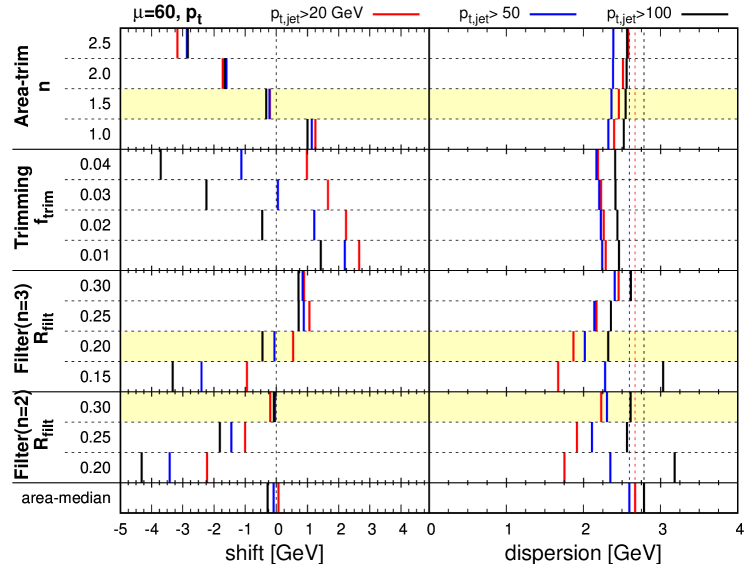
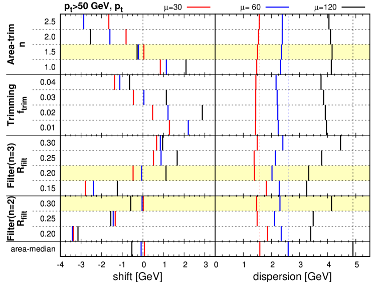
A summary of our findings is presented in Figs. 10.1 and 10.2. In both cases, we show the average shift and the corresponding dispersion for the different grooming techniques under scrutiny, varying their free parameter. In Fig. 10.1, we have fixed the pileup conditions to $\mu=60$ and varied the cut on the $p_{t}$ of the jet, while in fig. 10.2 we have worked with a fixed $p_{t}$ cut of 50 GeV and varied the pileup conditions.

The first properties we expect from an efficient pileup mitigation technique is that it remains unbiased and robust, i.e. that the average shift is close to 0 regardless of the pileup conditions and of the details of the hard process. In all cases, we see that this requirement is not trivially satisfied. At the very least, the free parameter of each grooming technique needs to be carefully tuned for the bias to remain small. This contrasts with the area–median approach where the average bias is very close to 0 in a wide variety of cases and where the free parameter, controlling the size of the patches, can be varied around the optimal scale without affecting significantly the performance.

Furthermore, we already see differences between the grooming methods at the level of the average bias. Filtering with $n_{\rm filt}=2$ and $R_{\rm filt}=0.3$, and area-trimming with $n_{\sigma}=1.5$ show small biases, comparable with the area–median approach, for all the cases we have studied. Then filtering with $n_{\rm filt}=3$ and $R_{\rm filt}=0.2$ shows a reasonably small bias albeit with a larger dependence on the pileup multiplicity. For trimming, the smallest bias is obtained for $f_{\rm trim}=0.03$ but this choice appears less robust that what we observe with other grooming techniques. Physically, this seems to indicate that if we want to use a method that decides which subjets are kept based on a $p_{t}$ cut, one obtains better results if the cut is set based on the pileup properties than based on the jet $p_{t}$. If some dependence on $p_{t}$ is to be included — e.g. to account for the residual biases of the area-trimming method — it should at least be milder than linear.

Turning to the dispersion, we see that the resolution degradation is, as expected, smaller than what one obtains with the area–median approach. We also see that the gain becomes larger as the pileup increases.

Figure 10.3: Plot of the average bias (left) and of the corresponding dispersion (right), as a function of the jet $p_{t}$ cut, for a few specific grooming techniques and for $\mu=60$,

Figure 10.4: Plot of the average bias (left) and of the corresponding dispersion (right), as a function of the average number of pileup interactions, for jets with $p_{t}>50$ GeV.

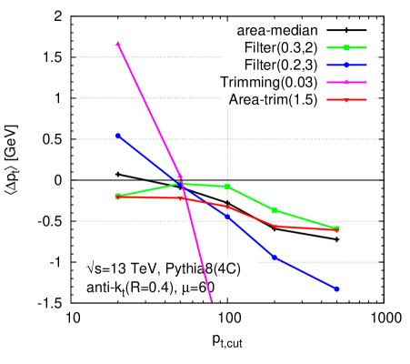
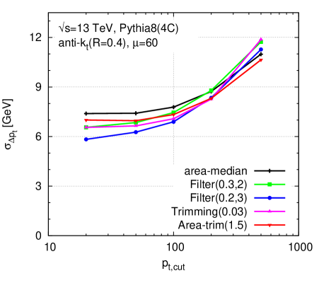
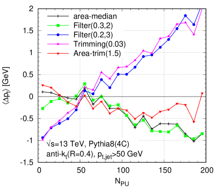
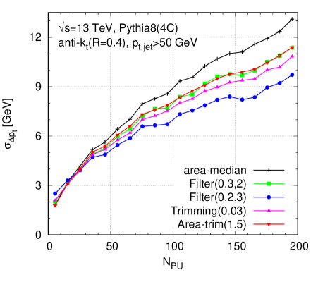
To investigate these results a bit further, we have selected for each of the 4 groomer families the one showing the best performance and we have looked more closely at the average shift and dispersion as a function of the jet $p_{t}$, Fig. 10.3, and of the pileup conditions, Fig. 10.4. This shows clearly that filtering with $n_{\rm filt}=2$ and $R_{\rm filt}=0.3$, and area-trimming with $n_{\sigma}=1.5$ have a bias similar to the area–median method, at least for the dijet processes that we have studied. Except for the filter at large $p_{t}$, these two options show an improvement over the area–median approach in terms of resolution degradation. At small $p_{t}$ (and $\mu=60$), we see an improvement around 5% for area-trimming and 15% for filtering. While this improvement persists across the whole $p_{t}$ range for the case of area-trimming, it disappears for $p_{t}\geq 200$ GeV in the case of filtering. This might not be too much of an issue since pileup is most problematic at low $p_{t}$. Nonetheless, it suggests that improvements are possible at large $p_{t}$. At high pileup multiplicities, both methods show a resolution improvement slightly above 10%.

If one wishes to tolerate a slightly larger bias, filtering with $n_{\rm filt}=3$ and $R_{\rm filt}=0.2$ can also be considered and gives a more sizeable improvement in terms of dispersion, although once again, this is mostly seen at small $p_{t}$.

10.4 Concluding remarks and future prospects

The study we have presented here is fairly minimal and definitely requires more tests if one wishes to draw a firm conclusion. We see however some patterns emerging:

• using grooming techniques as a tool for pileup subtraction requires some level of fine-tuning if one wishes to keep the average bias small.

• In the region where the bias is small, one sees, as initially foreseen, a reduction of the sensitivity to pileup fluctuations.

• Filtering with $n_{\rm filt}=2$ and $R_{\rm filt}=0.3$ or with $n_{\rm filt}=3$ and $R_{\rm filt}=0.2$ as well as the, new, area-trimming with $n_{\sigma}=1.5$ show overall good performances. Trimming seems to be disfavoured, in particular because it shows a larger dependence of the bias on the jet $p_{t}$.

The main message to remember from this preliminary pileup-mitigation study is that grooming can be a valuable tool in the context of pileup mitigation. It would also be interesting to carry further studies of the robustness of the methods that are seen to perform well here. This involves more detailed tests, including the rapidity dependence, a more complete scan over the jet $p_{t}$ and $N_{\mathrm{PU}}$ and the study of other processes, but also tests of detector effects or applications to CHS events (see also Chapter 11 and our final discussion in Chapter 14).

Finally, one may also consider dynamical adjustments of the parameters, e.g. $R_{\rm filt}$ or $n_{\sigma}$, with the jet $p_{t}$ and the pileup conditions. For example, we could groom more aggressively for low-$p_{t}$ jets where we see larger gains in terms of resolution and where these gains are the most important for practical applications at the LHC. Note that these parameters are expected to vary relatively slowly, typically only logarithmically, with the jet $p_{t}$.

Chapter 11 Using information from charged tracks

In this chapter, we consider the situation where we can use vertex information to tell whether a charged track comes from the hard interaction vertex of from a pileup vertex. We shall assume perfect identification and measurement of charged tracks and all vertices. This can be seen as an idealised Charge-Hadron-Subtracted (CHS) approach.

In this approach, the particles in each event can therefore be split in three main categories: neutral particles, charged particles from the hard interaction vertex, and charged particles from any of the pileup vertices. In that context, we can perform an exact subtraction of pileup for the charged part of the event, keeping the charged tracks associated with the leading vertex and discarding the ones associated with a pileup vertex. However, if one wishes to retain information from the charged particles associated with a pileup vertex, it is always possible to keep them as ghosts in the event, i.e. to keep them with transverse momenta scaled down to infinitesimal values. This is what we shall consider for most of our CHS-like events in what follows.

We are therefore left with the subtraction of the neutral part of the event. In this chapter, we investigate several methods that concentrate on pileup mitigation for CHS-type of events and compare their performance.

11.1 Pileup subtraction methods for CHS events

Area–median with charged-tracks information.

The generalisation of the area–median method to CHS events is straightforward: we simply compute $\rho$ (and $\rho_{m}$) as described in Section 2.4, this time using the particles from the CHS events. The rapidity profile can also be obtained from the neutral component of minimum bias. Note that, in practice, we could either use only the neutral particles or all CHS particles for the estimation of $\rho$. Since this makes very little difference in the end, we decided to compute the pileup density from all particles in the CHS event.

Furthermore, we still use (2.24) to subtract pileup from the jets. In the context of CHS events, we can also slightly improve our positivity constraints for the final jet transverse momentum and mass. If, after subtraction, the transverse momentum of the jet is less than the transverse momentum carried by charged tracks from the leading vertex, we set the subtracted 4-momentum to the sum of the charged tracks from the leading vertex. If it has a larger momentum but a smaller mass, we set the transverse momentum and azimuthal angle according to the result of the pileup subtraction and set the rapidity and mass as the one obtained from summing the charged tracks from the leading vertex. We shall study later in this chapter the effect of this “safe” subtraction on the reconstruction of the jet mass.

Note finally that, in FastJet, one can still use the Subtractor tool as for the standard usage. One can even use the Subtractor directly on full events using Subtractor::set_known_selectors(...) which takes two Selectors as arguments: the first one isolates particles which can be associated to a known vertex, while the second one selects the particles from the leading vertex among the particles with a known vertex association.

If we want to impose positivity constraints on the mass, we can still use Subtractor::set_safe_mass. With a previous call to Subtractor::set_known_selectors(...), the more constraining conditions, involving information from the particles associated with the leading vertex, will be used (see Section 2.4.4).

Neutral-proportional-to-charged (NpC).

An alternative approach to pileup subtraction in a context where we know for each charged track whether it comes from the leading vertex or from a pileup interaction is to deduce the neutral momentum of the jet based on its charged information. The NpC method estimates and subtracts the neutral pileup component by assuming it to be proportional to the charged pileup component. At least two variants can be conceived of.

If the charged pileup particles are kept (untouched) as part of the jet during clustering, then the corrected jet momentum is [143]

$$p_{\mu}^{\text{jet,sub}}=p_{\mu}^{\text{jet}}-\frac{1}{\gamma_{0}}p_{\mu}^{\text{jet,chg-PU}}\,,$$ (11.1)

where $p_{\mu}^{\text{jet,chg-PU}}$ is the four-momentum of the charged-pileup particles in the jet and $\gamma_{0}$ is the average fraction of pileup transverse momentum that is carried by charged particles. Specifically, one can define

$$\gamma_{0}\equiv\left\langle\frac{\sum_{i\in\text{charged particles}}\,p_{ti}}{\sum_{i\in\text{all particles}}\,p_{ti}}\right\rangle_{\text{\!\!events}}\!\!\!\!\!,$$ (11.2)

where the sums run over particles in a given event (possibly limited to some central region with tracking), and the average is carried out across minimum-bias events. With the Pythia 8 simulations we have used in this Chapter — see Section 11.2 below and Appendix E — we have $\gamma_{0}\approx 0.612$.

If the charged pileup particles are not directly included in the clustering (i.e. it is the CHS event that is provided to the clustering), then one needs to make sure that pileup vertices are still included as ghost tracks, with their momenta rescaled by an infinitesimal factor $\epsilon\lll 1$. In this case the correction becomes

$$p_{\mu}^{\text{jet,sub}}=p_{\mu}^{\text{jet,CHS}}-\frac{1-\gamma_{0}}{\gamma_{0}\,\epsilon}p_{\mu}^{\text{jet,rescaled-chg-PU}}\,,$$ (11.3)

where $p_{\mu}^{\text{jet,CHS}}$ is the momentum of the jet as obtained from the CHS event, while $p_{\mu}^{\text{jet,rescaled-chg-PU}}$ is the summed momentum of the rescaled charged-pileup particles that are in the jet. When carrying out NpC-style subtraction, this is our preferred approach because it eliminates any back-reaction associated with the charged pileup (this is useful also for the area–median subtraction), while retaining the information about charged pileup tracks.

There are multiple issues that may be of concern for the NpC method. For example, calorimeter fluctuations can limit the experiments’ ability to accurately remove the charged pileup component as measured with tracks. For out-of-time pileup, which contributes to calorimetric energy deposits, charged-track information may not be available at all. In any case, charged-track information covers only a limited range of detector pseudo-rapidities. Additionally there are subtleties with hadron masses: in effect, $\gamma_{0}$ is different for transverse components and for longitudinal components. In the following we will avoid this problem by treating all particles as massless. The importance of the above limitations can only be fully evaluated in an experimental context.

NpC also comes with a few potential (experimental) advantages compared to the area–median subtraction method. First, the area–median method includes questions of non-trivial rapidity dependence and detector non-linearities (the latter is relevant also for NpC). These have, to a reasonable extent, been successfully overcome by the experiments [144, 145]. One respect in which NpC may have advantages of the area–median method is that the latter fails to correctly account for the fact pileup fluctuates from point to point within the event, a feature that cannot be encoded within the global pileup estimate $\rho$. Furthermore NpC does not need a separate estimation of the background density $\rho$, which can have systematics related to the event structure (e.g. $t\bar{t}$ events v. dijet events); and there is no need to include large numbers of ghosts for determining jet areas, a procedure that has a non-negligible computational cost.

Jet cleansing.

Jet cleansing [11] essentially puts several ingredients together into a pileup subtraction technique. It first re-clusters the jet into subjets as done for filtering and trimming, see Sec. 6.2, (cf. also the early work by Seymour [146]). It then applies an NpC-like technique to each of the subjets, before summing the resulting 4-momenta into the final subtracted jet. It also applies an additional constraint that we decided to call zeroing and that we shall discuss separately later in this Section. Cleansing may also be used in conjunction with trimming-style cuts to the subtracted subjets, specifically it can remove those whose corrected transverse momentum is less than some fraction $f_{\text{cut}}$ of the overall jet’s transverse momentum (as evaluated before pileup removal).

To be a little more precise, the implementation of (linear) Jet Cleansing, available in fjcontrib, slightly differs from our definition of NpC. According to the description in Ref. [11], one additional characteristic of linear cleansing relative to NpC is that it switches to jet-vertex-fraction (JVF) cleansing when the NpC-style rescaling would give a negative answer. In contrast, area-subtraction plus trimming simply sets the (sub)jet momentum to zero. In our Monte-Carlo studies presented below in Section 11.2, we explicitly tried turning the switch to JVF-cleansing on and off and found it had a small effect and did not explain the differences.

Furthermore, Eq. (11.3) for NpC corrects for the jet 4-momentum, while cleansing scales the 4-momentum $p_{\mu}^{(i)}$ of each neutral particle $i$ in the jet as follows

$$p_{\mu}^{(i)}\;\to\;p_{\mu}^{(i)}\times\left(1-\frac{1-\gamma_{0}}{\gamma_{0}\epsilon}\frac{p_{t}^{\text{jet, rescaled-chg-PU}}}{p_{t}^{\text{jet, ntr}}}\right)\,,$$ (11.4)

where the notation is as in Eq. (11.3) and additionally $p_{t}^{\text{jet, ntr}}$ is the transverse momentum of the neutral part of the jet (including pileup). Eq. (11.4) is correct for the jet $p_{t}$, but would be only be correct for the jet mass if the pileup and hard components had identical angular distributions. However in practice, the hard component is usually collimated, whilst, to a first approximation, the pileup component is uniformly distributed across the jet. Accordingly, the scaling gives incorrect jet mass results. The issue is less severe when cleansing is used as originally intended, i.e. including trimming.

A last small difference is that cleansing assumes that all the particles in the event are clustered, in a spirit similar to Eq. (11.1). As already mentioned in our description of NpC, this can bring an additional source of back-reaction compared to Eq. (11.3), where the charged tracks from pileup vertices are only included as ghosts.

Note finally that besides the “linear” version of cleansing presented above, Ref. [11] also introduces a variant called Gaussian cleansing which is particularly interesting in that it effectively carries out a $\chi^{2}$ minimisation across different hypotheses for the ratio of charged to neutral energy flow, separately for the pileup and the hard event. We shall see below that its performance is usually marginally better than the much simpler linear cleansing.

Charged-tracks-based trimming, zeroing and protected zeroing.

It turns out that Jet Cleansing imposes an additional condition to subjets: if a subjet contains no charged particles from the leading vertex (LV), then its momentum is set to zero. Since we will be discussing it extensively, it is useful to give it a name, “zeroing”. Zeroing can be thought of as an extreme limit of the charged-track based trimming procedure introduced by ATLAS [148], whereby a JVF-style cut is applied to reject subjets whose charged-momentum fraction from the leading vertex is too low. As we will show in the Monte-Carlo studies presented in Section 11.2 zeroing turns out to be crucial in explaining the differences observed between CHS area-subtraction (or with NpC subtraction) with $f_{\text{cut}}=0$ trimming and cleansing.

This approach may seem a little dangerous since there are rare cases where a hard jet — or a subjet carrying a large fraction of the jet $p_{t}$ — can be purely neutral and zeroing would simply discard it. This can correspond to the loss of subjets with tens of GeV, while it is very unlikely that a subjet from a pileup collision will be responsible for such a large energy. Therefore we introduce a modified procedure that we call “protected zeroing”: one rejects any subjet without LV tracks unless its $p_{t}$ after subtraction is $n$ times larger than the largest charged $p_{t}$ in the subjet from any single pileup vertex (or, more simply, just above some threshold $p_{t,\text{min}}$; however, using $n$ times the largest charged subjet $p_{t}$ could arguably be better both in cases where one explores a wide range of $N_{\mathrm{PU}}$ and for situations involving a hard subjet from a pileup collision). We have found good results, and improvements compared to plain zeroing, taking $n=10$ (as we shall use later in our Monte-Carlo studies) or a fixed $p_{t,\text{min}}=20\,\mathrm{GeV}$.

Before starting an in-depth comparison of the methods described above, we also want to point out that similarly to the combination of a neutral-proportional-to-charged method with trimming, done by jet cleansing, several other similar approaches have been proposed and studied in the past in the context of the area–median approach[149]. We have already discussed in Chapter 4 (see also Ref.[6]) and in Chapter 7 (see also [38]) the possibility to combine the area–median subtraction together with grooming techniques and this combination can trivially be extended to the case of CHS events. The preliminary studies presented in Chapter 10 also relate to similar ideas.

11.2 Monte-Carlo studies and physical discussions

Since our testing framework remains close to the one we have used for the studies in Chapter 3, modulo a few adaptations meant to be closer to the setup used in Ref. [11], we will directly concentrate on the results of our studies and their physical interpretation. We refer to Appendix E for a more detailed description of our simulations.

Since the main goal of this Chapter is to discuss the use of charged tracks in pileup mitigation, the first and most important point we shall discuss is a comparison between the area–median method and the NpC approach. It will show that the former gives a slightly better performance than the latter and we will explain why this could be expected. We shall then discuss extensively the comparison of our findings with the, apparently contradictory, findings from jet cleansing in Ref. [11].

11.2.1 Performance of NpC v. area–median

Let us therefore proceed with an investigation of NpC’s performance compared to the now-familiar area–median method, focusing our attention on particle-level events for simplicity. The key question is the potential performance gain due to NpC’s use of local information. To study this quantitatively, we consider a circular patch of radius $R$ centred at $y=\phi=0$ and examine the correlation coefficient of the actual neutral energy flow in the patch with two estimates: (a) one based on the charged energy flow in the same patch and (b) the other based on a global energy flow determination from the neutral particles, $\rho_{\text{ntr}}$. Fig. 11.1 (left) shows these two correlation coefficients, “ntr v. chg” and “ntr v. $\rho_{\text{ntr}}A$”, as a function of $R$, for two average pileup multiplicities, $\mu=20$ and $\mu=100$. One sees that the local neutral-charged correlation is slightly lower, i.e. slightly worse, than the neutral-$\rho_{\text{ntr}}$ correlation. Both correlations decrease for small patch radii, as is to be expected, and the difference between them is larger at small patch radii. The correlation is largely independent of the number of pileup events being considered, which is consistent with our expectations, since all individual terms in the determination of the correlation coefficient should have the same scaling with $N_{\mathrm{PU}}$.

Figure 11.1: Left: the correlation coefficient between the neutral transverse momentum in a central patch and either the charged transverse momentum in that patch (rescaling this component would not change the correlation coefficient) or the prediction using the area–median method, i.e. $\rho_{\text{ntr}}A$. Right: the standard deviation of the difference between neutral transverse momentum in a central patch and either the rescaled charged transverse momentum in that patch or the prediction using the area–median method, i.e. $\rho_{\text{ntr}}A$. The events are composed of superposed zero-bias collisions simulated with Pythia 8, tune 4C, and the number of collisions per event is Poisson distributed with average $\mu$.

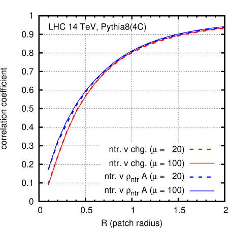
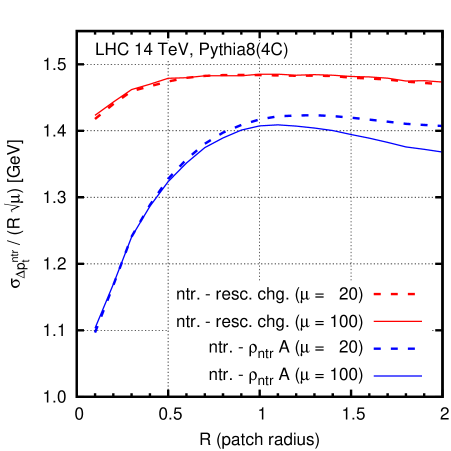
As already pointed out before, quantitative interpretations of correlation coefficients can sometimes be delicate (see also Appendix C). We instead find that it is more robust to investigate $\sigma_{\Delta p_{t}^{\text{ntr}}}$, defined (similarly to our previous studies in this document) as the standard deviation of

$$\Delta p_{t}^{\text{ntr}}=p_{t}^{\text{ntr}}-p_{t}^{\text{ntr,estimated}}\,,$$ (11.5)

where the estimate of neutral energy flow, $p_{t}^{\text{ntr,estimated}}$, may be either from the rescaled charged flow or from $\rho_{\text{ntr}}A$. The right-hand plot of Fig. 11.1 shows $\sigma_{\Delta p_{t}^{\text{ntr}}}$ for the two methods, again as a function of $R$, for two levels of pileup. It is normalised to $R\sqrt{\mu}$, to factor out the expected dependence on both the patch radius and the level of pileup. A lower value of $\sigma_{\Delta p_{t}^{\text{ntr}}}$ implies better performance, and as with the correlation we reach the conclusion that a global estimate of $\rho_{\text{ntr}}$ appears to be slightly more effective at predicting local neutral energy flow than does the local charged energy flow.

If one hoped to use NpC to improve on the performance of area–median subtraction, then figure 11.1 suggests that one will be disappointed: the local estimate of the neutral component of pileup from NpC is marginally worse than that given by the global $\rho_{\text{ntr}}$ from the area–median method.

In striving for an understanding of this finding, one should recall that the ratio of charged-to-neutral energy flow is almost entirely driven by non-perturbative effects. Inside an energetic jet, the non-perturbative effects are at scales $\sim\Lambda_{\text{QCD}}$ that are tiny compared to the jet transverse momentum $p_{t}$. There are fluctuations in the relative energy carried by charged and neutral particles, for example because a leading $u$-quark might pick up a $\bar{d}$ or a $\bar{u}$ from the vacuum. However, because $\Lambda_{\text{QCD}}\ll p_{t}$, the charged and neutral energy flow mostly tend to go in the same direction.

The case that we have just seen of an energetic jet gives an intuition that fluctuations in charged and neutral energy flow are going to be locally correlated. It is this intuition that motivates the study of NpC. We should however examine if this intuition is actually valid for pileup. We will examine one step of hadronisation, namely the production of short-lived hadronic resonances, for example a $\rho^{+}$. The opening angle between the $\pi^{+}\pi^{0}$ decay products of the $\rho^{+}$ is of order $2m_{\rho}/p_{t,\rho}$. Given that pileup hadrons are produced mostly at low $p_{t}$, say $0.5-2\,\mathrm{GeV}$, and that $m_{\rho}\simeq 0.77\,\mathrm{GeV}$, the angle between the charged and neutral pions ends up being of order $1$ or even larger. As a result, the correlation in direction between charged and neutral energy flow is lost, at least in part. Thus, at low $p_{t}$, non-perturbative effects specifically tend to wash out the charged-neutral angular correlation.

Figure 11.2: The filled histogram shows the distribution, for simulated zero-bias collisions, of the fraction, $r$, of the transverse momentum in a central circular patch of radius $R=0.4$ that is due to charged particles. It is separated into components according to the multiplicity of particles in the patch. The dashed and dotted histograms show the corresponding charged-fraction distributions for each of the two hardest anti-$k_{t}$, $R=0.4$ jets in simulated dijet events, with two choices for the hard generation cut $p_{t,\min}^{\text{gen}}$.

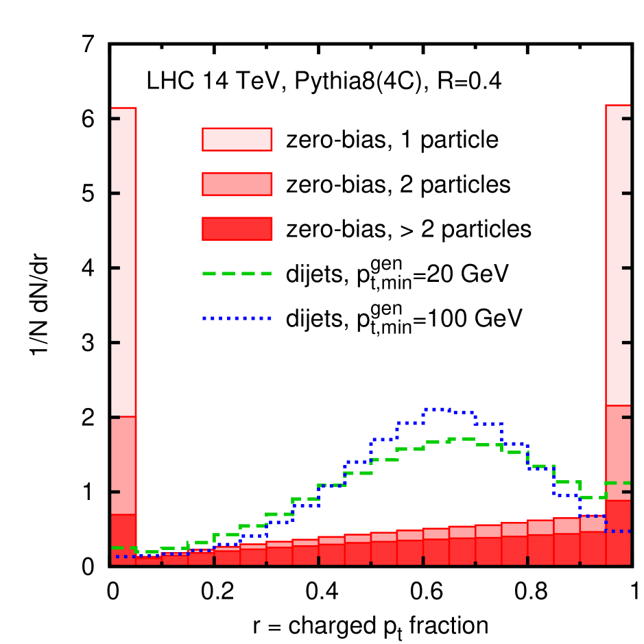
This point is illustrated in Fig. 11.2. We consider zero-bias events and examine a circular patch of radius $R=0.4$ centred at $y=\phi=0$. The figure shows the distribution of the charged $p_{t}$ fraction, $r$,

$$r=\frac{p_{t}^{\text{chg}}}{p_{t}^{\text{chg}+\text{ntr}}}\,,$$ (11.6)

in the patch (filled histogram, broken into contributions where the patch contains $1$, $2$ or more particles). The same plot also shows the distribution of the charged $p_{t}$ fraction in each of the two leading anti-$k_{t}$, $R=0.4$ jets in dijet events (dashed and dotted histograms). Whereas the charged-to-total ratio for a jet has a distribution peaked around $0.6$, as one would expect, albeit with a broad distribution, the result for zero-bias events is striking: in about 60% of events the patch is either just charged or just neutral, quite often consisting of just a single particle. This is probably part of the reason why charged information provides only limited local information about neutral energy flow in pileup events.

These considerations are confirmed by an analysis of the actual performance of NpC and area–median subtraction. We reconstruct jets using the anti-$k_{t}$ algorithm, as implemented in FastJet, with a jet radius parameter of $R=0.4$. We study dijet and pileup events generated with Pythia 8.176, in tune 4C; we assume idealised CHS, treating the charged pileup particles as ghosts. In the dijet (“hard”) event alone, i.e. without pileup, we run the jet algorithm and identify jets with absolute rapidity $|y|<2.5$ and transverse momentum $p_{t}>150\,\mathrm{GeV}$. Then in the event with superposed pileup (the “full” event) we rerun the jet algorithm and identify the jets that match those selected in the hard event and subtract them using either NpC, Eq. (11.3), or the area–median method, Eq. (2.24), with $\rho$ estimated from the CHS event. The hard events are generated with the underlying event turned off so as to avoid subtleties related to the simultaneous subtraction of the Underlying Event.

Figure 11.3: A comparison of the performance of the NpC and area–median subtraction methods. The left-hand plot shows, as a function of the number of pileup vertices $N_{\text{PU}}$, the average difference in $p_{t}$ between a jet after pileup addition and subtraction and the corresponding matched jet in the hard sample, $\Delta p_{t}=p_{t}^{\rm jet,sub}-p_{t}^{\rm jet,hard}$. The right-hand plot shows the standard deviation of $\Delta p_{t}$ (lower values are better). NpC is shown only for CHS events, while area–median subtraction is shown both for events with CHS and for events without it (“full”).

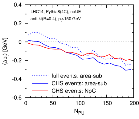
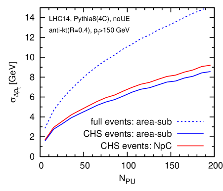
Figure 11.3 provides the resulting comparison of the performance of the NpC and area–median subtraction methods (the latter in CHS and in full events). The left-hand plot shows the average difference between the subtracted jet $p_{t}$ and the $p_{t}$ of the corresponding matched hard jet, as a function of the number of pileup interactions. Both methods clearly perform well here, with the average difference systematically well below $1\,\mathrm{GeV}$ even for very high pileup levels. The right-hand plot shows the standard deviation of the difference between the hard and subtracted full jet $p_{t}$. A lower value indicates better performance, and one sees that in CHS events the area–median method indeed appears to have a small, but consistent advantage over NpC. Comparing area–median subtraction in CHS and full events, one observes a significant degradation in resolution when one fails to use the available information about charged particles in correcting the charged component of pileup, as is to be expected for a particle-level study.

The conclusion of this section is that the NpC method fails to give a superior performance to the area–median method in CHS events. This is because the local correlations of neutral and charged energy flow are no greater than the correlations between local neutral energy flow and the global energy flow. We believe that part of the reason for this is that the hadronisation process for low $p_{t}$ particles intrinsically tends to produce hadrons separated by large angles, as illustrated concretely in the case of $\rho^{\pm}$ resonance decay.

11.2.2 Performance of cleansing v. area–median

Figure 11.4: Upper left plot: the dispersion of $\Delta m_{jj}=m_{jj}^{\text{sub}}-m_{jj}^{\text{hard}}$ after adding pileup and applying various pileup-removal methods; shown as a function of the number of pileup events, $N_{\text{PU}}$. Upper right plot: similarly for the single jet mass. Both plots are for a hadronically decaying $Z^{\prime}$ sample with $m_{Z^{\prime}}=500\,\mathrm{GeV}$. Decays are included to all flavours except $t\bar{t}$ and $B$-hadrons are taken stable. Lower-left plot: the dispersion of $\Delta m_{jj}$, as in the upper-left plot, but with a sample of $Z^{\prime}$ bosons that decay only to $u$, $d$ and $s$ quarks. Jets are reconstructed, as in Ref. [11], with the anti-$k_{t}$ algorithm with $R=1$. For both trimming and cleansing, subjets are reconstructed with the $k_{t}$ algorithm with $R_{\text{sub}}=0.3$ and the $f_{\text{cut}}$ value that is applied is $f_{\text{cut}}=0$.

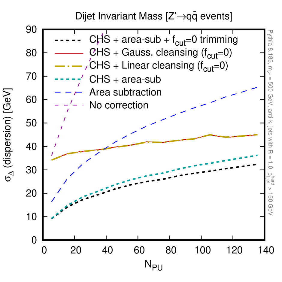
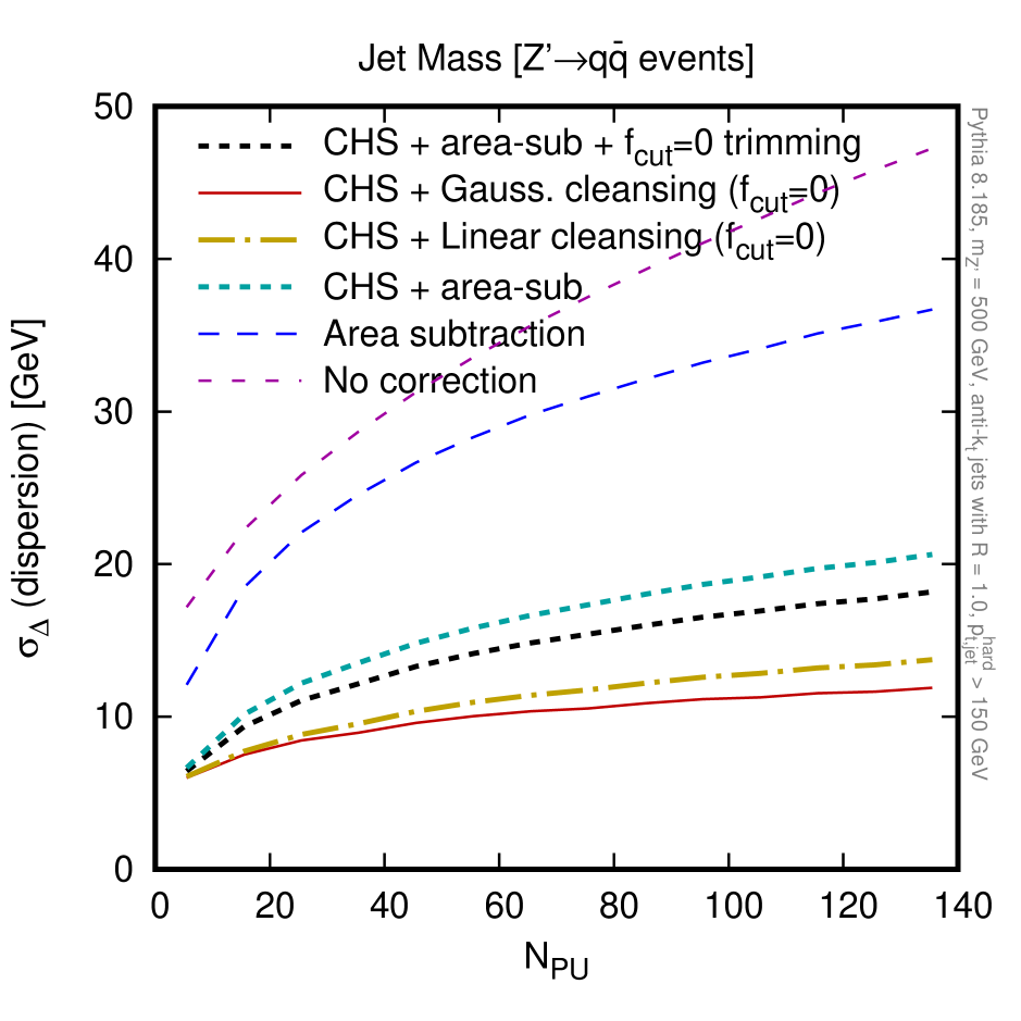
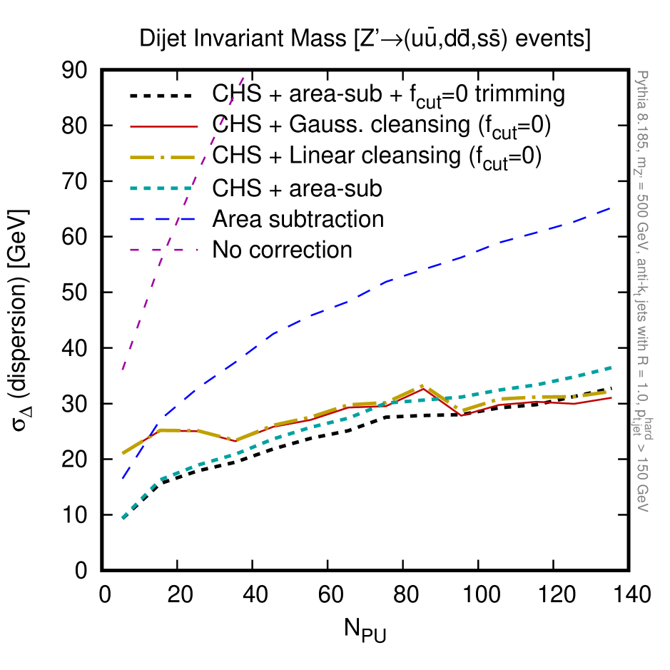
We now turn to a broader discussion, comparing our discussion about the NpC and area–median approaches with the results found using Jet Cleansing.

The top left-hand plot of Fig. 11.4 shows the dispersion $\Delta m_{jj}=m_{jj}^{\text{sub}}-m_{jj}^{\text{hard}}$ for the dijet mass for several pileup mitigation methods. The results are shown as a function of $N_{\mathrm{PU}}$. The pileup mitigation methods include two forms of cleansing (with $f_{\text{cut}}=0$), area–median subtraction, CHS+area subtraction, and CHS+area subtraction in conjunction with trimming (also with $f_{\text{cut}}=0$). The top right-hand plots shows the corresponding results for the jet mass. For the dijet mass we see that linear (and Gaussian) cleansing performs worse than area subtraction, while in the right-hand plot, for the jet mass, we see linear (and Gaussian) cleansing performing better than area subtraction, albeit not to the extent found in Ref. [11]. These (and, unless explicitly stated, our other $Z^{\prime}$ results) have been generated with the $Z^{\prime}$ decaying to all flavours except $t\bar{t}$, and $B$-hadrons have been kept stable. The lower plot shows the dijet mass for a different $Z^{\prime}$ sample, one that decays only to $u$, $d$ and $s$ quarks, but not $c$ and $b$ quarks. Most of the results are essentially unchanged. The exception is cleansing, which turns out to be very sensitive to the sample choice. Without stable $B$-hadrons in the sample, its performance improves noticeably and at high pileup becomes comparable to that of area-subtraction.

In light of our results on NpC in section 11.2.1, the difference between the performance of area-subtraction plus trimming versus that of cleansing are puzzling: our expectation is that their performances should be similar. The strong sample-dependence of the cleansing performance also calls for an explanation. We thus pursue with an in-depth study of the question.

As mentioned in our description of cleansing in Section 11.1, one additional characteristic of linear cleansing relative to area-subtraction is that it switches to jet-vertex-fraction (JVF) cleansing when the NpC-style rescaling would give a negative answer. In contrast, area-subtraction plus trimming simply sets the (sub)jet momentum to zero. We explicitly tried turning the switch to JVF-cleansing on and off and found it had a small effect and did not explain the differences observed in Fig. 11.4.

The next difference that we will discuss at length is the zeroing step that we introduced in Section 11.1. Zeroing turns out to be crucial: if we use it in conjunction with CHS area-subtraction (or with NpC subtraction) and $f_{\text{cut}}=0$ trimming, we obtain results that are very similar to those from cleansing. Conversely, if we turn this step off in linear-cleansing, its results come into accord with those from (CHS) area-subtraction or NpC-subtraction with $f_{\text{cut}}=0$ trimming.

To help illustrate this, Fig. 11.5 shows a “fingerprint” for each of several pileup-removal methods, for both the jet $p_{t}$ (left) and mass (right). The fingerprint includes the average shift ($\langle\Delta p_{t}\rangle$ or $\langle\Delta m\rangle$) of the observable after pileup removal, shown in black. It also includes two measures of the width of the $\Delta p_{t}$ and $\Delta m$ distributions: the dispersion (i.e. standard deviation) in red and an alternative peak-width measure in blue. The latter is defined as follows: one determines the width of the smallest window that contains $90\%$ of the entries and then scales this width by a factor $0.304$. For a Gaussian distribution, the rescaling ensures that the resulting peak-width measure is equal to the dispersion. For a non-Gaussian distribution the two measures usually differ and the orange shaded region quantifies the extent of this difference. The solid black, blue and red lines have been obtained from samples in which the $Z^{\prime}$ decays just to light quarks; the dotted lines are for a sample including $c\bar{c}$ and $b\bar{b}$ decays (with stable $B$-hadrons), providing an indication of the sample dependence; in many cases they are indistinguishable from the solid lines.

Comparing $f_{\text{cut}}=0$ grooming for NpC, area (without zeroing) and cleansing with zeroing manually disabled, all have very similar fingerprints. Turning on zeroing in the different methods leads to a significant change in the fingerprints, but again NpC, area and cleansing are very similar.

Figure 11.5: The left-hand plot illustrates various characteristics of the change ($\Delta p_{t}$) in the jet $p_{t}$ after addition of pileup and removal by a range of methods. It shows the average shift $\langle\Delta p_{t}\rangle$ (in black) and the peak width (in blue) and dispersion (in red) of the $\Delta p_{t}$ distribution. The peak width is defined as the smallest window of $\Delta p_{t}$ that contains 90% of the $\Delta p_{t}$ distribution, scaled by a factor $\simeq 0.304$ such that in the case of a Gaussian distribution the result agrees with the dispersion. The right-hand plot shows the same set of results for the jet mass. The results are obtained in a sample of events with the number of pileup vertices distributed uniformly between $0$ and $140$. The hard events consist of hadronic $Z^{\prime}$ decays: for the solid vertical lines the sample is $Z^{\prime}\to d\bar{d},u\bar{u},s\bar{s}$, while for the dotted lines (sometimes not visible because directly over the solid lines), the sample additionally includes $Z^{\prime}\to c\bar{c},b\bar{b}$ with $B$ hadrons kept stable. The $Z^{\prime}$ mass is $m_{Z^{\prime}}=500\,\mathrm{GeV}$ and jets are reconstructed with the anti-$k_{t}$ algorithm with $R=1$. All results in this figure include charged-hadron subtraction by default. The default form of cleansing, as used e.g. in Fig. 11.4, is “$f_{\text{cut}}=0$ zeroing”.

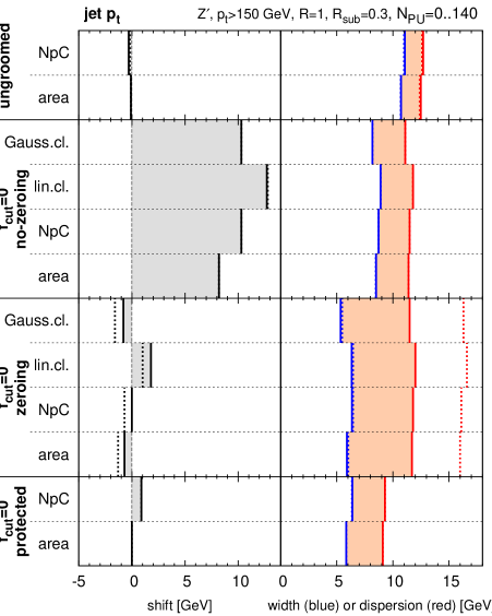
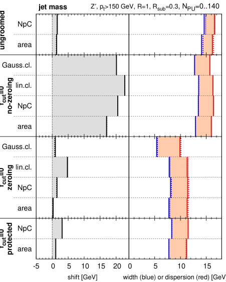
When used with $f_{\text{cut}}=0$ trimming, and when examining quality measures such as the dispersion (in red, or the closely related correlation coefficient, cf. Appendix C), subjet zeroing appears to be advantageous for the jet mass, but potentially problematic for the jet $p_{t}$ and the dijet mass. However, the dispersion quality measure does not tell the full story regarding the impact of zeroing. Examining simultaneously the peak-width measure (in blue) makes it easier to disentangle two different effects of zeroing. On one hand we find that zeroing correctly rejects subjets that are entirely due to fluctuations of the pileup. This narrows the peak of the $\Delta p_{t}$ or $\Delta m$ distribution, substantially reducing the (blue) peak-width measures in Fig. 11.5. On the other hand, zeroing sometimes incorrectly rejects subjets that have no charged tracks from the LV but do have significant neutral energy flow from the LV. This can lead to long tails for the $\Delta p_{t}$ or $\Delta m$ distributions, adversely affecting the dispersion. It is the interplay between the narrower peak and the longer tails that affects whether overall the dispersion goes up or down with zeroing. In particular the tails appear to matter more for the jet $p_{t}$ and dijet mass than they do for the single-jet mass. Note that accurate Monte Carlo simulation of such tails may be quite challenging: they appear to be associated with configurations where a subjet contains an unusually small number of energetic neutral particles. Such configurations are similar to those that give rise to fake isolated photons or leptons and that are widely known to be difficult to simulate correctly.

We commented earlier that the cleansing performance has a significant sample dependence. This is directly related to the zeroing: indeed Fig. 11.5 shows that for cleansing without zeroing, the sample dependence (dashed versus solid lines) vanishes, while it is substantial with zeroing. Our understanding of this feature is that the lower multiplicity of jets with undecayed $B$-hadrons (and related hard fragmentation of the $B$-hadron) results in a higher likelihood that a subjet will contain neutral but no charged particles from the LV, thus enhancing the impact of zeroing on the tail of the $\Delta p_{t}$ or $\Delta m_{jj}$ sample.

The long tails produced by the zeroing can be avoided by using the alternative protected zeroing described in Section 11.1. Taking $n=10$ (or a fixed $p_{t,\text{min}}=20\,\mathrm{GeV}$) we have found reduced tails and, consequently, noticeable improvements in the jet $p_{t}$ and dijet mass dispersion (with little effect for the jet mass). This is visible for area and NpC subtraction in Fig. 11.5. Protected zeroing also eliminates the sample dependence.

Several additional comments can be made about $f_{\text{cut}}=0$ trimming combined with zeroing. Firstly, $f_{\text{cut}}=0$ trimming alone introduces a bias in the jet $p_{t}$, which is clearly visible in the $f_{\text{cut}}=0$ no-zeroing shifts in Fig. 11.5. This is because the trimming removes negative fluctuations of the pileup, but keeps the positive fluctuations. Zeroing then counteracts that bias by removing some of the positive fluctuations, those that happened not to have any charged tracks from the LV. It also introduces further negative fluctuations for subjets that happened to have some neutral energy flow but no charged tracks. Overall, one sees that the final net bias comes out to be relatively small. This kind of cancellation between different biases is common in noise-reducing pileup-reduction approaches [151, 152, 153, 12, 13] as we have already seen in Chapter 10 and will see again in the next two Chapters of this review.

Figure 11.6: Left, Analogue of Fig. 11.5 (left) for a jet radius of $R=0.4$, subjet radius (where relevant) of $R_{\text{sub}}=0.2$ and a QCD continuum dijet sample generated with Pythia 8. The underlying event is turned off in the sample and $B$ hadrons decay. We consider only jets that in the hard sample have $p_{t}>50\,\mathrm{GeV}$ and $|y|<2.5$. Right: the dispersions for a subset of the methods, shown as a function of the number of pileup events.

Figure 11.7: Analogue of Fig. 11.5 (right), showing the performance for the jet mass, but now with $f_{\text{cut}}=0.05$ applied to both trimming and cleansing and in a sample of hadronically-decaying boosted $W$ bosons ($pp\to W^{+}W^{-}$). The jets reconstructed after addition and subtraction of pileup are compared to trimmed hard jets. Jets are reconstructed with a jet radius of $R=1$ and a subjet radius of $R_{\text{sub}}=0.3$. Only hard jets with $p_{t}>500\,\mathrm{GeV}$ and $|y|<2.5$ (before trimming) are considered and we let $B$ hadrons decay.

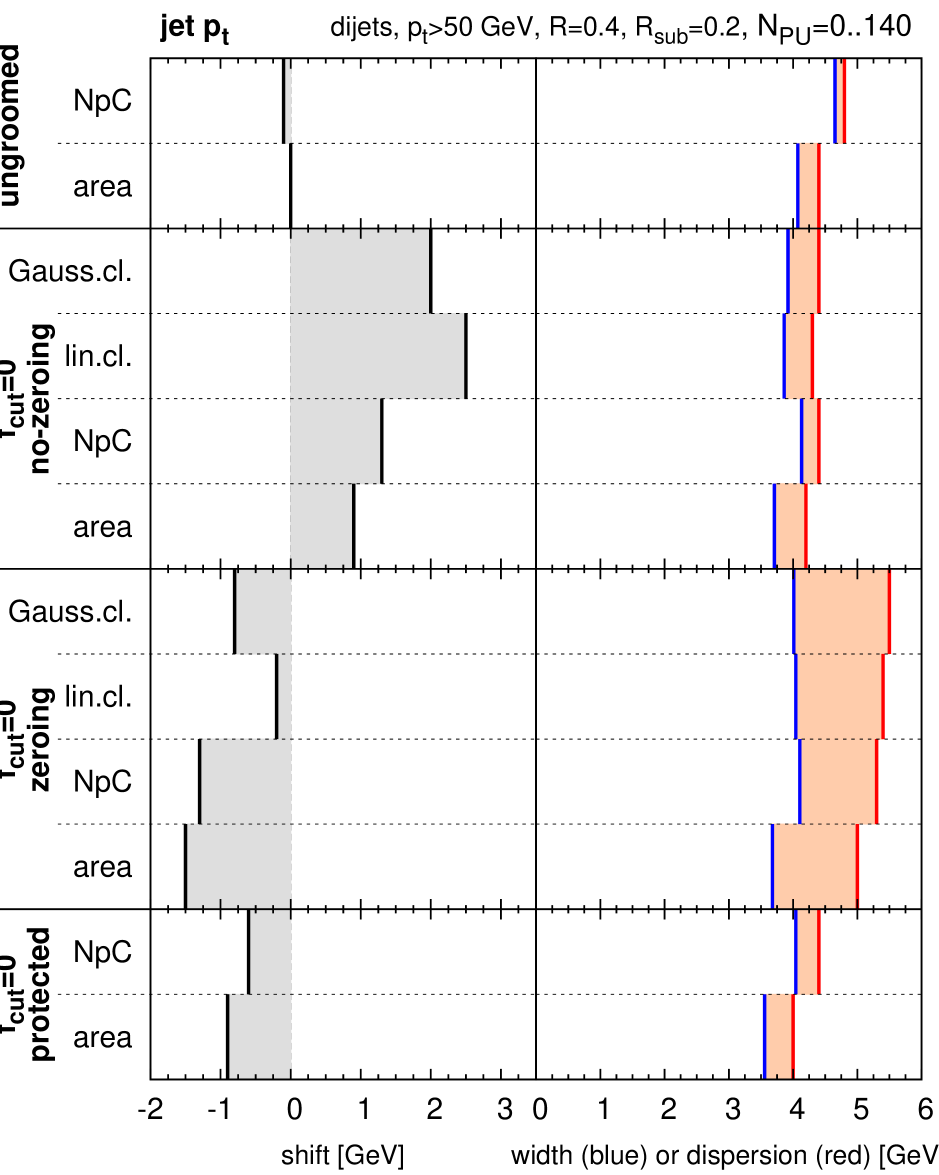
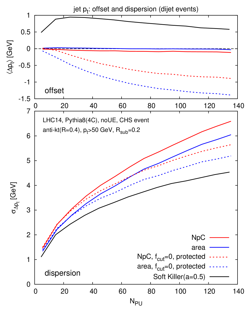
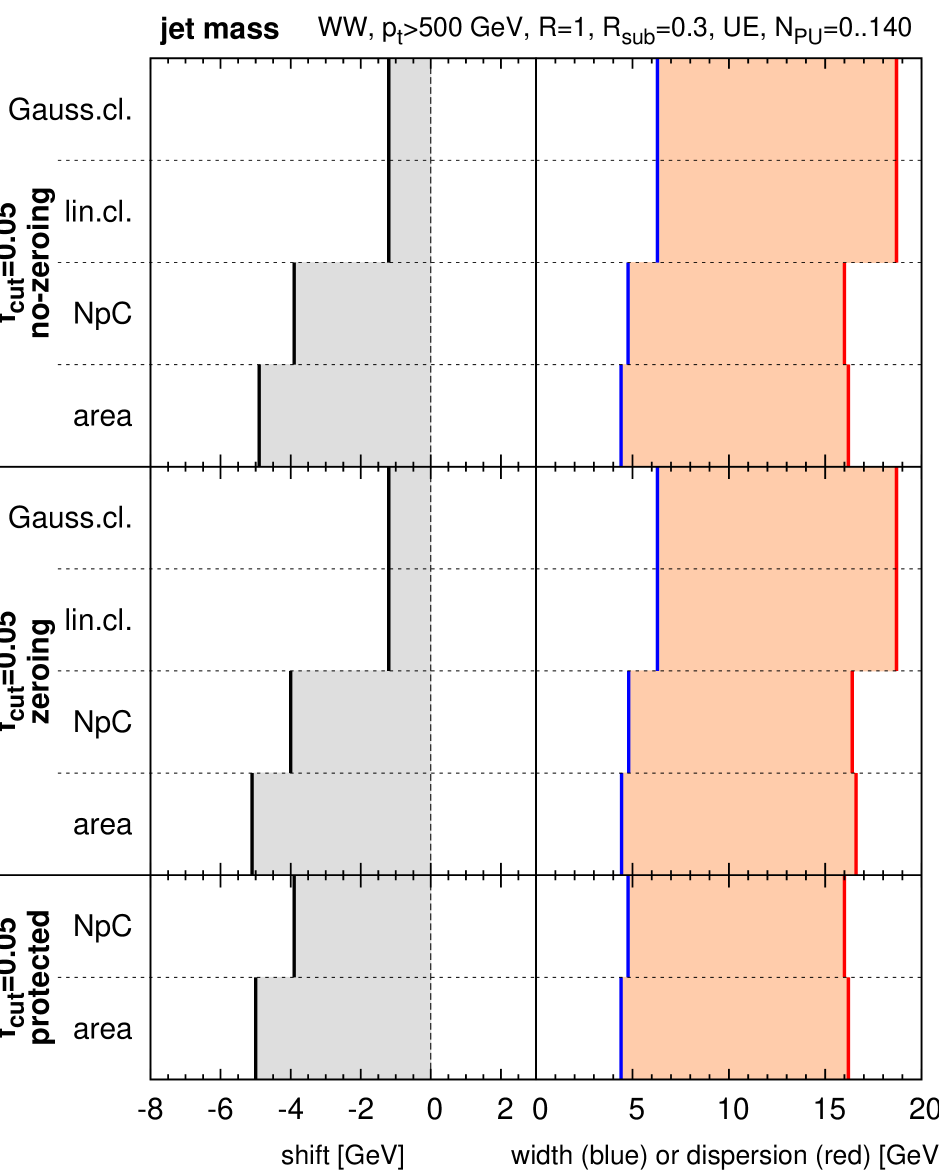
Most of the studies so far in this section have been carried out with a setup that is similar to that of Ref. [11], i.e. $R=1$ jets in a $Z^{\prime}$ sample with $f_{\text{cut}}=0$ trimming. This is not a common setup for most practical applications. For most uses of jets, $R=0.4$ is a standard choice and pileup is at its most severe at low to moderate $p_{t}$. Accordingly, in Fig. 11.6 (left) we show the analogue of Fig. 11.5’s summary for the jet $p_{t}$, but now for $R=0.4$, with $R_{\text{sub}}=0.2$ in a QCD dijet sample, considering jets that in the hard event had $p_{t}>50\,\mathrm{GeV}$. We see that qualitatively the pattern is quite similar to that in Fig. 11.5, with the area–median approach performing slightly better than NpC-based techniques as expected from our discussion in Section 11.2.1. Quantitatively, the difference between the various choices is much smaller, with about a $10\%$ reduction in dispersion (or width) in going from ungroomed CHS area-subtraction to the $f_{\text{cut}}=0$ protected subjet-zeroing case. One should be aware that this study is only for a single $p_{t}$, across a broad range of pileup. The dispersions for a subset of the methods are shown as a function of the number of pileup vertices in the right-hand plot of Fig. 11.6. That plot also includes results from the SoftKiller method discussed in Chapter 12 (see also [12]) and illustrates that the benefit from protected zeroing (comparing the solid and dashed blue curves) is about half of the benefit that is brought from SoftKiller (comparing solid blue and black curves). These plots show that protected zeroing is potentially of interest for jet $p_{t}$ determinations in realistic conditions. Thus it would probably benefit from further study: one should, for example, check its behaviour across a range of transverse momenta, determine optimal choices for the protection of the zeroing and investigate also how best to combine it with particle-level subtraction methods such as SoftKiller. We will come back to this combination in Section 13.2.

Turning now to jet masses, the use of $R=1$ is a not uncommon choice, however most applications use a groomed jet mass with a non-zero $f_{\text{cut}}$ (or its equivalent): this improves mass resolution in the hard event even without pileup, and it also reduces backgrounds, changing the perturbative structure of the jet [135, 139] even in the absence of pileup. Accordingly in Fig. 11.7 we show $f_{\text{cut}}=0.05$ results (with shifts and widths computed relative to $f_{\text{cut}}=0.05$ trimmed hard jets) for a hard $WW$ sample where the hard fat jets are required to have $p_{t}>500\,\mathrm{GeV}$. Zeroing, whether protected or not, appears to have little impact. One potential explanation for this fact is as follows: zeroing’s benefit comes primarily because it rejects fairly low-$p_{t}$ pileup subjets that happen to have no charged particles from the leading vertex. However for a pileup subjet to pass the $f_{\text{cut}}=0.05$ filtering criterion in our sample, it would have to have $p_{t}>25\,\mathrm{GeV}$. This is quite rare. Thus filtering is already removing the pileup subjets, with little further to be gained from the charged-based zeroing. As in the plain jet-mass summary plot, protection of zeroing appears to have little impact for the trimmed jet mass. Does that mean that (protected) zeroing has no scope for improving the trimmed-jet mass? The answer is “not necessarily”: one could for example imagine first applying protected zeroing to subjets on some angular scale $R_{\text{zero}}$ in order to eliminate low-$p_{t}$ contamination; then reclustering the remaining constituents on a scale $R_{\text{trim}}\gtrsim R_{\text{zero}}$, subtracting according to the area or NpC methods, and finally applying the trimming momentum cut (while also keeping in mind the considerations of footnote 14). In that context, it would also be interesting to consider the combination of zeroing with the grooming techniques suggested as pileup mitigation methods in Chapter 10.

Further systematic comparisons of the different methods, with and without zeroing can be found in the Appendices of Ref. [10].

We close this section with a summary of our findings. Based on its description in Ref. [11] and our findings about NpC v. area subtraction, cleansing with $f_{\text{cut}}=0$ would be expected to have a performance very similar to that of CHS+area subtraction with $f_{\text{cut}}=0$ trimming. The differences in behaviour between (linear) cleansing and trimmed CHS+area-subtraction therefore call for an explanation, and appear to be due to a step in the cleansing code that was undocumented in Ref. [11] and that we dubbed “zeroing”: if a subjet contains no charged tracks from the leading vertex it is discarded. Zeroing is an extreme form of a procedure described in Ref. [148]. In can be used also with area or NpC subtraction, and we find that it brings a benefit for the peak of the $\Delta p_{t}$ and $\Delta m$ distributions, but appears to introduce long tails in $\Delta p_{t}$. A variant, “protected zeroing”, can avoid the long tails by still accepting subjets without leading-vertex tracks, if their $p_{t}$ is above some threshold, which may be chosen dynamically based on the properties of the pileup. In our opinion, a phenomenologically realistic estimate of the benefit of zeroing (protected or not) requires study not of $R=1$ plain jets, but instead of $R=0.4$ jets (for the jet $p_{t}$) or larger-$R$ trimmed jets with a non-zero $f_{\text{cut}}$ (for the jet mass). In a first investigation, there appear to be some phenomenological benefits from protected zeroing for the $R=0.4$ jet $p_{t}$, whereas to obtain benefits for large-$R$ trimmed jets would probably require further adaptation of the procedure. In any case, additional study is required for a full evaluation of protected zeroing and related procedures.

11.3 Digression: combining different methods

Figure 11.8: Left: correlation between $p_{t}^{\text{ntr}}-\hat{p}_{\mu}^{\text{ntr(NpC)}}$ and $p_{t}^{\text{ntr}}-\hat{p}_{\mu}^{\text{ntr(${\rho}A$)}}$, shown as a function of $R$. Right: optimal weight $f$ for combining NpC and area pileup subtraction, Eq. (11.9), as a function of $R$.

Figure 11.9: Comparison of the performance of NpC, area–median and combined subtraction, as a function of the number of pileup vertices. The left-hand plot is for the jet $p_{t}$ and the right-hand one for the jet mass.

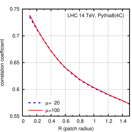
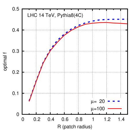
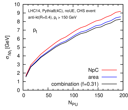
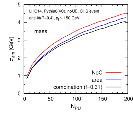
It is interesting to further probe the relation between NpC and the area–median method and to establish whether there might be a benefit from combining them: the area–median method makes a mistake in predicting local energy flow mainly because local energy flow fluctuates from region to region; NpC makes a mistake because charged and neutral energy flow are not $100\%$ locally correlated. The key question is whether, for a given jet, NpC and the area–median method generally make the same mistake, or if instead they are making uncorrelated mistakes. In the latter case it should be possible to combine the information from the two methods to obtain an improvement in subtraction performance.

Let $p_{t}^{\text{ntr}}$ be the actual neutral pileup component flowing into a jet, while

$$\hat{p}_{\mu}^{\text{ntr(NpC)}}=\frac{1-\gamma_{0}}{\gamma_{0}\epsilon}p_{\mu}^{\text{jet,rescaled-chg-PU}}\,,\qquad\hat{p}_{\mu}^{\text{ntr(${\rho}A$)}}={\rho}A\,,$$ (11.7)

are, respectively, the estimates for the neutral pileup based on the local charged $p_{t}$ flow and on ${\rho}A$. Note that we for our analysis in this section we use CHS events and in particular ${\rho}$ is as determined from the CHS event, i.e. $\rho\equiv\rho_{\text{CHS}}$. This means that it is essentially equal to $\rho_{\text{ntr}}$, with small differences arising principally due to the presence of the charged component of the LV’s underlying event contribution. One could of course also use the actual $\rho_{\text{ntr}}$ instead of $\rho_{\text{CHS}}$ to estimate $\hat{p}_{\mu}^{\text{ntr(${\rho}A$)}}$, and this would in some respects be a more coherent approach, though the numerical differences will be small.

Concentrating on the transverse components, the extent to which the two estimates in Eq. (11.7) provide complementary information can be quantified in terms of (one minus) the correlation coefficient, $r$, between $p_{t}^{\text{ntr}}-\hat{p}_{\mu}^{\text{ntr(NpC)}}$ and $p_{t}^{\text{ntr}}-\hat{p}_{\mu}^{\text{ntr(${\rho}A$)}}$. That correlation is shown as a function of $R$ in Fig. 11.8 (left), and it is quite high, in the range $0.6$–$0.7$ for commonly used $R$ choices. It is largely independent of the number of pileup vertices.

Let us now quantify the gain to be had from a linear combination of the two prediction methods, i.e. using an estimate

$$\hat{p}_{\mu}^{\text{ntr}}=f\hat{p}_{\mu}^{\text{ntr(NpC)}}+(1-f)\hat{p}_{\mu}^{\text{ntr(${\rho}A$)}}\,,$$ (11.8)

where $f$ is to be chosen to as to minimise the dispersion of $p_{t}^{\text{ntr}}-\hat{p}_{t}^{\text{ntr}}$. Given dispersions $\sigma_{\text{NpC}}$ and $\sigma_{{\rho}A}$ respectively for $p_{t}^{\text{ntr}}-\hat{p}_{\mu}^{\text{ntr(NpC)}}$ and $p_{t}^{\text{ntr}}-\hat{p}_{\mu}^{\text{ntr(${\rho}A$)}}$, we can show that the optimal $f$ is

$$f=\frac{\sigma_{{\rho}A}^{2}-r\,\sigma_{\text{NpC}}\,\sigma_{{\rho}A}}{\sigma_{\text{NpC}}^{2}+\sigma_{{\rho}A}^{2}-2r\,\sigma_{\text{NpC}}\,\sigma_{{\rho}A}}\,,$$ (11.9)

which is plotted as a function of $R$ in Fig. 11.8 (right). The resulting squared dispersion for $p_{t}^{\text{ntr}}-\hat{p}_{t}^{\text{ntr}}$ is

$$\sigma^{2}=\frac{(1-r^{2})\,\sigma_{\text{NpC}}^{2}\,\sigma_{{\rho}A}^{2}}{\sigma_{\text{NpC}}^{2}+\sigma_{\rho A}^{2}-2r\,\sigma_{\text{NpC}}\,\sigma_{{\rho}A}}\,.$$ (11.10)

Reading $r=0.67$ from Fig. 11.8 (left) for $R=0.4$, and $\sigma_{\text{NpC}}\simeq 1.14\,\sigma_{{\rho}A}$ from Fig. 11.1 (right), one finds $f\simeq 0.31$ and $\sigma\simeq 0.96\,\sigma_{{\rho}A}$. Because of the substantial correlation between the two methods, ones expects only a modest gain from their linear combination.

In Fig. 11.9 we compare the performance of pileup subtraction from the combination of the NpC and the area–median methods, using the optimal value $f=0.31$ that can be read from Fig. 11.8 (right) for $R=0.4$, both for the jet $p_{t}$ and the jet mass. The expected small gain is indeed observed for the jet $p_{t}$, and it is slightly larger for the jet mass. Given the modest size of the gain, one may wonder how phenomenologically relevant it is likely to be. Nevertheless, one might still consider investigating whether the gain carries over also to a realistic experimental environment with full detector effects.

Note finally that the approach described above can be applied to combine a different pair of pileup mitigation techniques. It can also easily be extended to more than two methods.

11.4 Concluding remarks and discussions

One natural approach to pileup subtraction is to use the charged pileup particles in a given jet to estimate the amount of neutral pileup that needs to be removed from that same jet. In this chapter, with the help of particle-level simulations, we have studied such a method (NpC) and found that it has a performance that is similar to, though slightly worse than the existing, widely used area–median method. This can be related to the observation that the correlations between local charged and neutral energy flow are no larger than those between global and local energy flow. Tentatively, we believe that this is in part because the non-perturbative effects that characterise typical inelastic proton-proton collisions act to destroy local charged-neutral correlation.

When studying cleansing, we have seen an improved performance for the jet mass. This improvement may come as a surprise since cleansing is largely based on Npc. We trace a key difference in the behaviour of cleansing and area subtraction (or pure NpC) to the use in the cleansing code of a step that was not documented in Ref. [11] and that discards subjets that contain no tracks from the leading vertex. This “zeroing” step, similar to the charged-track based trimming introduced by ATLAS [148], can indeed be of benefit. It has a drawback of introducing tails in some distributions due to subjets with a substantial neutral $p_{t}$ from the leading vertex, but no charged tracks. As a result, different quality measures (and different event samples) lead to different conclusions as to the benefits of zeroing. The tails can be alleviated by a variant of zeroing that we introduce in Ref. [10], “protected zeroing”, whereby subjets without LV charged tracks are rejected only if their $p_{t}$ is below some (possibly pileup-dependent) threshold. Protected zeroing does in some cases appear to have phenomenological benefits, which are observed across all quality measures.

Code for the above implementation of area subtraction with positive-definite mass is available as part of FastJet versions 3.1.0 and higher (see Section 2.7 and, in particular, 2.7.2.4). Public code and samples for carrying out a subset of the comparisons with cleansing described in section 11.2.2, including also the NpC subtraction tools, are available from Ref. [154].

To conclude this Chapter, we want to point out that NpC and cleansing are not the only ways to use charged-track information in the context of jet clustering and pileup mitigation. For example, one could simply imagine clustering jets using only the charged tracks in the event, for which an almost perfect separation between the leading vertex and pileup interactions can be performed. One could then scale the result to mimic the inclusion of the neutral contribution to the jets. In this context where we are dominated by the high-$p_{t}$ dynamics of jets, we expect a much larger correlation between charged and neutral particles than what was seen in Section 11.2.1 for soft pileup particles. Furthermore, for idealised CHS events for which tracks from the leading vertex can be exactly identified, such a rescaling would be independent of the pileup conditions. However, this would result in fluctuations which scale with the $p_{t}$ of the jet rather than the, much softer, $\sigma\sqrt{A_{\text{jet}}}$ scale driving fluctuations in the area–median subtraction. Unless $p_{t}$ is very small and $N_{\mathrm{PU}}$ very large this is therefore not practical.

Charged tracks could be used when designing more elaborate pileup mitigation techniques which rely on additional kinematic properties of the jets and of the event in general. If these kinematic properties are the same (or very similar) for charged and neutral particles, one could then obtain them directly from the data. The determination of the “$\alpha$ distribution” used in the PUPPI method is an illustration of this (see Fig. 1 of Ref. [142]). Similarly, one could imagine determining the SoftKiller grid-size parameter (see the next Chapter) based on an estimation using charged tracks.

Chapter 12 Noise reduction with the SoftKiller

In this Chapter, we describe a new method that we introduced in Ref. [12] and that we called SoftKiller (SK). This method acts as a noise-reduction method which has shown nice resolution improvements compared to the area–median method in Monte-Carlo simulations.

We will first describe the method itself in Section 12.1 followed by some validation in Monte-Carlo studies (Section 12.2) as well as possible adaptations to specific situations like CHS events and detector effects (Section 12.3).

One of the interesting features of the SoftKiller method is that it shows remarkable performance in terms of computing time. We will discuss that in Section 12.4.

The work presented in this Chapter is a minor adaptation of the original SoftKiller paper  [12]. We will discuss in the next Chapter, devoted to preliminary ideas and results, some possible ways to further improve the SoftKiller method.

12.1 The SoftKiller method

The SoftKiller method involves eliminating particles below some $p_{t}$ cutoff, $p_{t}^{\text{cut}}$, chosen to be the minimal value that ensures that $\rho$ is zero. Here, $\rho$ is the event-wide estimate of transverse-momentum flow density in the area–median approach, i.e. given by Eq. (2.23). In practice we will use a grid-base estimate for $\rho$.

Figure 12.1: Illustration of the SoftKiller method. The left plot depicts particles in an event, with the hard event particles shown in blue and the pileup particles shown in red. On the right, the same event after applying the SoftKiller. The vertical dotted lines represent the edges of the patches used to estimate the pileup density $\rho$.

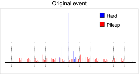
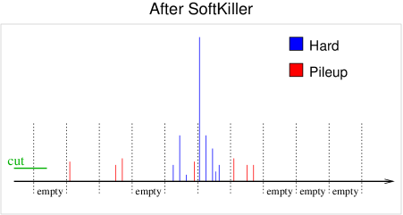
Choosing the minimal transverse momentum threshold, $p_{t}^{\text{cut}}$, that results in $\rho=0$ is equivalent to gradually raising the $p_{t}$ threshold until exactly half of the patches contain no particles, which ensures that the median is zero. This is illustrated in Fig. 12.1. Computationally, $p_{t}^{\text{cut}}$ is straightforward to evaluate: one determines, for each patch $i$, the $p_{t}$ of the hardest particle in that patch, $p_{ti}^{\max}$ and then $p_{t}^{\text{cut}}$ is given by the median of $p_{ti}^{\max}$ values:

$$p_{t}^{\text{cut}}=\underset{i\in\text{patches}}{\text{median}}\left\{p_{ti}^{\max}\right\}\,.$$ (12.1)

With this choice, half the patches will contain only particles that have $p_{t}<p_{t}^{\text{cut}}$. These patches will be empty after application of the $p_{t}$ threshold, leading to a zero result for $\rho$ as defined in Eq. (2.23). The computational time to evaluate $p_{t}^{\text{cut}}$ as in Eq. (12.1) scales linearly in the number of particles and the method should be amenable to parallel implementation.

Imposing a cut on particles’ transverse momenta eliminates most of the pileup particles, and so might reduce the fluctuations in residual pileup contamination from one point to the next within the event. However, as with other event-wide noise-reducing pileup and underlying-event mitigation approaches, notably the CMS heavy-ion method [151, 152, 153] (cf. the analysis in Appendix A.4 of Ref. [80]; see also our introductory discussion in Chapter 9), the price that one pays for noise reduction is the introduction of biases. Specifically, some particles from pileup will be above $p_{t}^{\text{cut}}$ and so remain to contaminate the jets, inducing a net positive bias in the jet momenta. Furthermore some particles in genuine hard jets will be lost, because they are below the $p_{t}^{\text{cut}}$, inducing a negative bias in the jet momenta. The jet energy scale will only be correctly reproduced if these two kinds of bias are of similar size, so that they largely cancel. There will be an improvement in the jet resolution if the fluctuations in these biases are modest.

Figure 12.2: Left: value of the $p_{t}$ cut applied by the SoftKiller, displayed as a function of the number of pileup events. We show results for two different values of the generator minimal $p_{t}$ for the hard event, $p_{t,\rm gen}$. The solid line is the average $p_{t}^{\text{cut}}$ value while the dashed lines indicate the one-standard-deviation band. Right: plot of the $p_{t}$ that is lost when applying a given $p_{t}$ cut (the $x$ axis) to the constituents of jets clustered (anti-$k_{t}$, $R=0.4$) from the hard event (solid lines) and the residual pileup $p_{t}$ that remains after applying that same cut to the constituents of circular patches of radius $0.4$ in pure-pileup events (dashed lines).

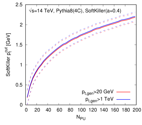
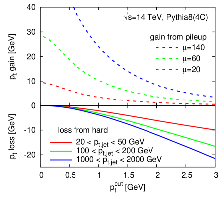
Figure 12.2 shows, on the left, the average $p_{t}^{\text{cut}}$ value, together with its standard deviation (dashed lines), as a function of the number of pileup interactions, ${N_{\mathrm{PU}}}$. The event sample consists of a superposition of ${N_{\mathrm{PU}}}$ zero-bias on one hard dijet event, in 14 TeV proton–proton collisions, all simulated with Pythia 8 (tune 4C) [55]. The underlying event in the hard event has been switched off, and all particles have been made massless, maintaining their $p_{t}$, rapidity and azimuth. These are our default choices throughout this Chapter. The grid used to determine $p_{t}^{\text{cut}}$ has a spacing of $a\simeq 0.4$ and extends up to $|y|<5$. One sees that $p_{t}^{\text{cut}}$ remains moderate, below $2\,\mathrm{GeV}$, even for pileup at the level foreseen for the high-luminosity upgrade of the LHC (HL-LHC), which is expected to reach an average (Poisson-distributed) number of pileup interactions of $\mu\simeq 140$. The right-hand plot shows the two sources of bias: the lower (solid) curves, illustrate the bias on the hard jets induced by the loss of genuine hard-event particles below $p_{t}^{\text{cut}}$. Jet clustering is performed as usual with the anti-$k_{t}$ jet algorithm with $R=0.4$ (as implemented in FastJet 3.1). The three line colours correspond to different jet $p_{t}$ ranges. The loss has some dependence on the jet $p_{t}$ itself, notably for higher values of $p_{t}^{\text{cut}}$. In particular it grows in absolute terms for larger jet $p_{t}$’s, though it decreases relative to the jet $p_{t}$. The positive bias from residual pileup particles (calculated in circular patches of radius $0.4$ at rapidity $y=0$) is shown as dashed curves, for three different pileup levels. To estimate the net bias, one should choose a value for ${N_{\mathrm{PU}}}$, read the average $p_{t}^{\text{cut}}$ from the left-hand plot, and for that $p_{t}^{\text{cut}}$ compare the solid curve with the dashed curve that corresponds to the given ${N_{\mathrm{PU}}}$. Performing this exercise reveals that there is indeed a reasonable degree of cancellation between the positive and negative biases. Based on this observation, we can move forward with a more detailed study of the performance of the method.

12.2 SoftKiller performance

Choice of grid size.

For a detailed study of the SoftKiller method, the first step is to choose the grid spacing $a$ so as to break the event into patches. The spacing $a$ is the one main free parameter of the method. The patch-size parameter is present also for area–median pileup subtraction. There the exact choice of this parameter is not too critical because the median is quite stable when pileup levels are high: all grid cells are filled, and nearly all are dominated by pileup. However the SoftKiller method chooses the $p_{t}^{\text{cut}}$ so as to obtain a nearly empty event. In this limit, the median operation becomes somewhat more sensitive to the grid spacing (see also the discussion in Section 5.2).

Fig. 12.3 considers a range of hard event samples (different line styles) and pileup levels (different colours). For each, as a function of the grid spacing $a$, the left-hand plot shows the average, $\langle\Delta p_{t}\rangle$, of the net shift in the jet transverse momentum, defined as before

$$\Delta p_{t}=p_{t}^{\text{corrected}}-p_{t}^{\text{hard}}\,,$$ (12.2)

while the right-hand plot shows the dispersion, $\sigma_{\Delta p_{t}}$, of that shift from one jet to the next, here normalised to $\sqrt{\mu}$ (right).

Figure 12.3: Scan of the SoftKiller performances as a function the grid-spacing parameter $a$ for different hard-event samples and three different pileup levels (Poisson-distributed with average pileup event multiplicities of $\mu=20,60,140$). Left: average $p_{t}$ shift; right: $p_{t}$ shift dispersion, normalised to $\sqrt{\mu}$ for better readability. Results are given for a variety of hard processes and pileup conditions to illustrate robustness. Curves labelled $p_{t}>X$ correspond to dijet events, in which one studies only those jets that in the hard event have a transverse momentum greater than $X$. For the $t\bar{t}$ sample, restricted to fully hadronic decays of the top quarks, the study is limited to jets that have $p_{t}>50\,\mathrm{GeV}$ in the hard event.

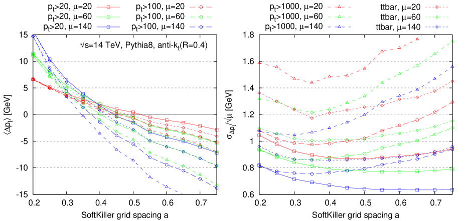
One sees that the average jet $p_{t}$ shift has significant dependence on the grid spacing $a$. However, there exists a grid spacing, in this case $a\simeq 0.4$, for which the shift is not too far from zero and not too dependent either on the hard sample choice or on the level of pileup. In most cases the absolute value of the shift is within about $2\,\mathrm{GeV}$, the only exception being for the $p_{t}>1000\,\mathrm{GeV}$ dijet sample, for which the bias can reach up to $4\,\mathrm{GeV}$ for $\mu=140$. This shift is, however, still less than the typical best experimental systematic error on the jet energy scale, today of the order of $1\%$ or slightly better [157, 158].

It is not trivial that there should be a single grid spacing that is effective across all samples and pileup levels: the fact that there is can be considered phenomenologically fortuitous. The value of the grid spacing $a$ that minimises the typical shifts is also close to the value that minimises the dispersion in the shifts. That optimal value of $a$ is not identical across event samples, and can also depend on the level of pileup. However the dispersion at $a=0.4$ is always close to the actual minimal attainable dispersion for a given sample. Accordingly, for most of the rest of this article, we will work with a grid spacing of $a=0.4$.

Figure 12.4: Performance of SoftKiller for 50 GeV jets and $\mu=60$ Poisson-distributed pileup events. We plot the distribution of the shift $\Delta p_{t}$ between the jet $p_{t}$ after pileup removal and the jet $p_{t}$ in the hard event alone. Results are compared between the area–median approach and the SoftKiller. For comparison, the (orange) dash-dotted line corresponds to the situation where no pileup corrections are applied.

Figure 12.5: Performance of SoftKiller shown as a function of the pileup multiplicity and compared to the area–median subtraction method. Left: the average $p_{t}$ shift after subtraction, compared to the original jets in the hard event. Right: the corresponding dispersion.

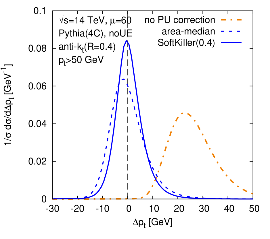
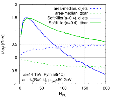
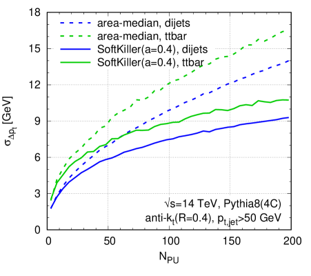
Performance compared to the area–median method.

We now compare the performance of the SoftKiller to that of area–median subtraction. Figure 12.4 shows the distribution of shift in $p_{t}$, for (hard) jets with $p_{t}>50\,\mathrm{GeV}$ in a dijet sample. The average number of pileup events is $\mu=60$, with a Poisson distribution. One sees that in the SoftKiller approach, the peak is about $30\%$ higher than what is obtained with the area–median approach and the distribution correspondingly narrower. The peak, in this specific case, is well centred on $\Delta p_{t}=0$.

Figure 12.5 shows the shift (left) and dispersion (right) as a function of ${N_{\mathrm{PU}}}$ for two different samples: the $p_{t}>50\,\mathrm{GeV}$ dijet sample (in blue), as used in Fig. 12.4, and a hadronic $t\bar{t}$ sample, with a $50\,\mathrm{GeV}$ $p_{t}$ cut on jets (in green). Again, the figure compares the area–median (dashed) and SoftKiller results (solid). One immediately sees that the area–median approach gives a bias that is more stable as a function of ${N_{\mathrm{PU}}}$. Nevertheless, the bias in the SoftKiller approach remains between about $-0.5$ and $1.5\,\mathrm{GeV}$, which is still reasonable when one considers that, experimentally, some degree of recalibration is anyway needed after area–median subtraction. As concerns sample dependence of the shift, comparing $t\bar{t}$ v. dijet, the area–median and SoftKiller methods appear to have similar systematic differences. In the case of SoftKiller, there are two main causes for the sample dependence: firstly the higher multiplicity of jets has a small effect on the choice of $p_{t}^{\text{cut}}$ and secondly the dijet sample is mostly composed of gluon-induced jets, whereas the $t\bar{t}$ sample is mostly composed of quark-induced jets (which have fewer soft particles and so lose less momentum when imposing a particle $p_{t}$ threshold). Turning to the right-hand plot, with the dispersions, one sees that the SoftKiller brings a significant improvement compared to area–median subtraction for ${N_{\mathrm{PU}}}\gtrsim 20$. The relative improvement is greatest at high pileup levels, where there is a reduction in dispersion of $30-35\%$, beating the $\sqrt{{N_{\mathrm{PU}}}}$ scaling that is characteristic of the area–median method. While the actual values of the dispersion depend a little on the sample, the benefit of the SoftKiller approach is clearly visible for both.

Figure 12.6: Performance of SoftKiller shown as a function of the hard jet $p_{t}$ (solid lines), with a comparison to the area–median subtraction method (dashed lines). Left: the average shifts for the jet $p_{t}$ (blue) and mass (green), after subtraction. Right: the corresponding dispersions.

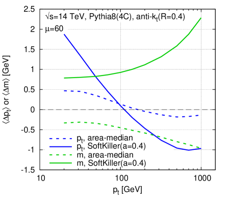
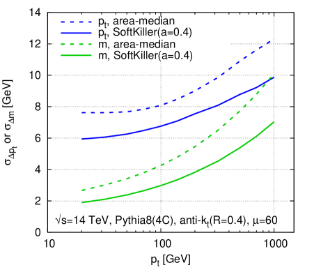
Figure 12.6 shows the shift (left) and dispersion (right) for jet $p_{t}$’s and jet masses, now as a function of the hard jet minimum $p_{t}$. Again, dashed curves correspond to area–median subtraction, while solid ones correspond to the SoftKiller results. All curves correspond to an average of $60$ pileup interactions. For the jet $p_{t}$ (blue curves) one sees that the area–median shift ranges from $0.5$ to $0\,\mathrm{GeV}$ as $p_{t}$ increases from $20\,\mathrm{GeV}$ to $1\,\mathrm{TeV}$, while for SK the dependence is stronger, from about $2$ to $-1\,\mathrm{GeV}$, but still reasonable. For the jet mass (green curves), again the area–median method is more stable than SK, but overall the biases are under control, at the $1$ to $2\,\mathrm{GeV}$ level. Considering the dispersions (right), one sees that SK gives a systematic improvement, across the whole range of jet $p_{t}$’s. In relative terms, the improvement is somewhat larger for the jet mass ($\sim 30\%$) than for the jet $p_{t}$ ($\sim 20\%$).

Figure 12.7: Performance of SoftKiller on jet mass reconstruction. We show the jet mass distribution after applying different pileup mitigation techniques. Left: dijet events, right: hadronically-decaying $t\bar{t}$ events.

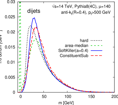
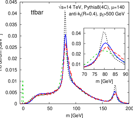
Fig. 12.7 shows the actual mass spectra of $R=0.4$ jets, for two samples: a QCD dijet sample and a boosted $t\bar{t}$ sample. For both samples, we only considered jets with $p_{t}>500\,\mathrm{GeV}$ in the hard event. One sees that SK gives slightly improved mass peaks relative to the area–median method and also avoids area–median’s spurious peak at $m=0$, which is due to events in which the squared jet mass came out negative after four-vector area-subtraction and so was reset to zero. The plot also shows results from the recently proposed Constituent Subtractor method [28], using v. 1.0.0 of the corresponding code from FastJet Contrib [159]. It too performs better than area–median subtraction for the jet mass, though the improvement is not quite as large as for SK.

Figure 12.8: The results of the SoftKiller and other methods applied to large-$R$ jets. The left-hand plot is without grooming, the right-hand plot with grooming (trimming with $R_{\text{trim}}=0.2$ and $f_{\text{cut}}=0.05$).

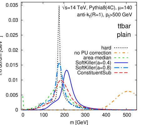
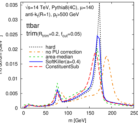
Large-$R$ jets and grooming.

One might ask why we concentrated on $R=0.4$ jets here, given that jet-mass studies often use large-$R$ jets. The reason is that large-$R$ jets are nearly always used in conjunction with some form of grooming, for example trimming, pruning or filtering (see also Chapter 6). Grooming reduces the large-radius jet to a collection of small-radius jets and so the large-radius groomed-jet mass is effectively a combination of the $p_{t}$’s and masses of one or more small-radius jets.

For the sake of completeness, let us briefly also study the SoftKiller performance for large-$R$ jets. Figure 12.8 shows jet-mass results for the same $t\bar{t}$ sample as in Fig. 12.7 (right), now clustered with the anti-$k_{t}$ algorithm with $R=1$. The left-hand plot is without grooming: one sees that SK with our default spacing of $a=0.4$ gives a jet mass that has better resolution than area–median subtraction (or the ConstituentSubtractor), but a noticeable shift, albeit one that is small compared to the effect of uncorrected pileup. That shift is associated with some residual contamination from pileup particles: in an $R=0.4$ jet, there are typically a handful of particles left from pileup, which compensate low-$p_{t}$ particles lost from near the core of the jet. If one substantially increases the jet radius without applying grooming, then that balance is upset, with substantially more pileup entering the jet, while there is only slight further loss of genuine jet $p_{t}$. To some extent this can be addressed by using the SoftKiller with a larger grid spacing (cf. the $a=0.8$ result), which effectively increases the particle $p_{t}^{\text{cut}}$. This comes at the expense of performance on small-$R$ jets (cf. Fig. 12.3). An interesting, open problem is to find a simple way to remove pileup from an event such that, for a single configuration of the pileup removal procedure, one simultaneously obtains good performance on small-$R$ and large-$R$ jets. We will come back to candidate solutions to this open question in Chapter 13 (Section 13.2.1).

As we said above, however, large-$R$ jet masses are nearly always used in conjunction with some form of grooming. Fig. 12.8 (right) shows that when used together with trimming, SoftKiller with our default $a=0.4$ choice performs well both in terms of resolution and shift.

Figure 12.9: Performance of the SoftKiller on jet shapes, compared to area–median subtraction and the recently proposed Constituent Subtractor method [28]. All results are shown for dijet events with a 500 GeV $p_{t}$ cut on anti-$k_{t}$, $R=0.4$ jets. For comparison of the subtraction performance we also quote, for each observable $X$, $\sigma_{X,\rm hard}$, the dispersion of the distribution of the observable in the hard event. For $\tau_{21}$ there is the additional requirement (in the hard event) that the jet mass is above 30 GeV and for $\tau_{32}$ we further impose that $\tau_{21}\geq 0.1$ (again in the hard event), so as to ensure infrared safety.

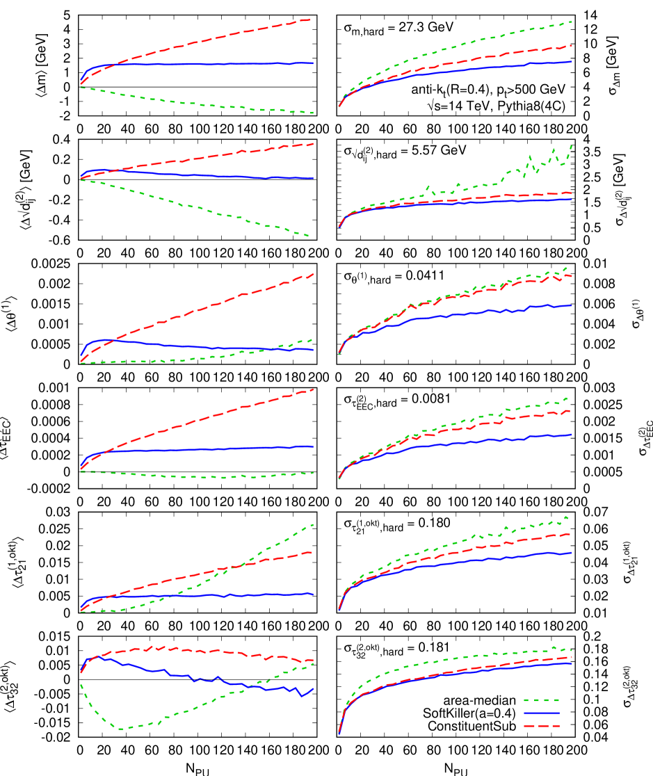
Jet shapes.

Returning to $R=0.4$ jets, the final figure of this section, Fig. 12.9, shows average shifts (left) and dispersions (right) as a function of ${N_{\mathrm{PU}}}$ for several different jet “shapes”: jet masses, $k_{t}$ clustering scales [45, 46], the jet width (or broadening or girth [160, 65, 66]), an energy–energy correlation moment [71] and the $\tau_{21}^{(\beta=1)}$ and $\tau_{32}^{(\beta=2)}$ N-subjettiness ratios [74, 75], using the exclusive $k_{t}$ axes with one-pass of minimisation. Except in the case of the jet mass (which uses “safe” area subtraction, as mentioned above), the area–median results have been obtained using the shape subtraction technique introduced in Section 2.5, as implemented in v. 1.2.0 of the GenericSubtractor in FastJet Contrib.

As regards the shifts, the SK approach is sometimes the best, other times second best. Which method fares worst depends on the precise observable. In all cases, when considering the dispersions, it is the SK that performs best, though the extent of the improvement relative to other methods depends strongly on the particular observable. Overall this figure gives us confidence that one can use the SoftKiller approach for a range of properties of small-radius jets.

Rapidity dependence.

Given that the SoftKiller imposes a fixed $p_{t}$ cut, one might wonder if it correctly account for the rapidity dependence of pileup. In the case of the area–median subtraction, that is handled by the rapidity rescaling used in Eq. (2.27) which we have used throughout this Chapter. The rapidity dependence of $\rho$ is shown as the dashed lines in Fig. 12.10 (left) for two different tunes (4C and Monash 2013), illustrating the fact that they have somewhat different rapidity dependence.

Figure 12.10: Left: rapidity dependence, in simulated zero-bias events, of the $p_{t}$ density per unit area ($\rho(y)$), and of the average $p_{t}$ per particle (scaled by a factor of $2$ for readability), comparing Pythia 8’s 4C and Monash 2013 [161] tunes. Right: the average shift in jet $p_{t}$ as a function of rapidity for the area–median method with rapidity rescaling (our default), without rapidity rescaling, and for the SoftKiller.

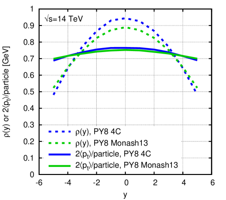
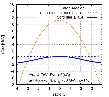
The SoftKiller method acts not on the average energy flow, but instead on the particle $p_{t}$’s. The solid lines in Fig. 12.10 (left) show that the average particle $p_{t}$ is nearly independent of rapidity. This suggests that there may not be a need to explicitly account for rapidity in the SK method, at least at particle level (detector effects introduce further non-trivial rapidity dependence).

This is confirmed in the right-hand plot of Fig. 12.10, which shows the rapidity-dependence of the shift in the jet $p_{t}$ with the area–median and SK methods. Our default area–median curve, which includes rapidity rescaling, leads to a nearly rapidity-independent shift. However, without the rapidity rescaling, there are instead rapidity-dependent shifts of up to $10\,\mathrm{GeV}$ at high pileup. In contrast, the SK method, which in our implementation does not involve any parametrisation of rapidity dependence, automatically gives a jet $p_{t}$ shift that is fairly independent of rapidity, to within about $2\,\mathrm{GeV}$. We interpret this as a consequence of the fact (cf. the left-hand plot of Fig. 12.10) that the average particle $p_{t}$ appears to be far less dependent on rapidity than the average $p_{t}$ flow. In a similar spirit to (2.27), one could also imagine introducing a rapidity-dependent rescaling of the particle $p_{t}$’s before applying SoftKiller, and then inverting the rescaling afterwards. Our initial tests of this approach suggest that it does largely correct for the residual SK rapidity dependence.

12.3 Adaptation to CHS events and calorimetric events

It is important to verify that the SoftKiller (or any other new pileup mitigation method with noise reduction) works not just at particle level, but also at detector level, essentially to make sure that the balance between the positive and negative biases discussed in Section 12.1 is not spoiled. There are numerous subtleties in carrying out detector-level simulation, from the difficulty of correctly treating the detector response to low-$p_{t}$ particles, to the reproduction of actual detector reconstruction methods and calibrations, and even the determination of which observables to use as performance indicators. Here we will consider two cases: idealised charged-hadron-subtraction, which simply examines the effect of discarding charged pileup particles; and simple calorimeter towers.

Performance on CHS events.

As in the previous Chapter, for events with particle flow [162] and charged-hadron subtraction (CHS), we imagine a situation in which all charged particles can be unambiguously associated either with the leading vertex or with a pileup vertex. We then apply the SK exclusively to the neutral particles, which we assume to have been measured exactly. This is almost certainly a crude approximation, however it helps to illustrate some general features.

Figure 12.11: Same as Fig. 12.5, for events with charged-hadron subtraction (CHS). Note that the grid size used for the SoftKiller curves has been set to $a=0.5$.

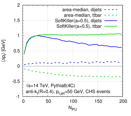
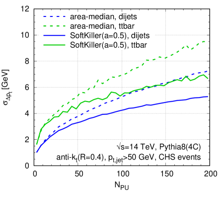
One important change that arises from applying SK just to the neutral particles is that there is a reduced contribution of low-$p_{t}$ hard-event particles. This means that for a given actual amount of pileup contamination (in terms of visible transverse momentum per unit area), one can afford to cut more aggressively, i.e. raise the $p_{t}^{\text{cut}}$ as compared to the full particle-level case, because for a given $p_{t}^{\text{cut}}$ there will be a reduced loss of hard-event particles. This can be achieved through a moderate increase in the grid spacing, to $a=0.5$. Figure 12.11 shows the results, with the shift (left) and dispersion (right) for the jet $p_{t}$ in dijet and $t\bar{t}$ samples. The SK method continues to bring an improvement, though that improvement is slightly more limited than in the particle-level case. We attribute this reduced improvement to the fact that SK’s greatest impact is at very high pileup, and for a given ${N_{\mathrm{PU}}}$, SK with CHS is effectively operating at lower pileup levels than without CHS. In Ref. [12], Appendix E, we also carried on a further study with our toy CHS simulation concerning lepton isolation.

Performance with calorimetric events.

Next let us turn to events where the particles enter calorimeter towers. Here we encounter the issue (discussed also in Appendix F) that SK is not collinear safe. While we argue there that this is not a fundamental drawback from the point of view of particle-level studies, there are issues at calorimeter level: on one hand a single particle may be divided between two calorimeter towers (we will not attempt to simulate this, as it is very sensitive to detector details); on the other, within a given tower (say $0.1\times 0.1$) it is quite likely that for high pileup the tower may receive contributions from multiple particles. In particular, if a tower receives contributions from a hard particle with a substantial $p_{t}$ and additionally from pileup particles, the tower will always be above threshold, and the pileup contribution will never be removed. There are also related effects due to the fact that two pileup particles may enter the same tower. To account for the fact that towers have finite area, we therefore adapt the SK as follows. In a first step we subtract each tower:

$$p_{t}^{\text{tower,sub}}=\max\left(0,\;p_{t}^{\text{tower}}-\rho A^{\text{tower}}\right)\,,$$ (12.3)

where $\rho$ is as determined on the event prior to any correction. This in itself eliminates a significant fraction of pileup, but there remains a residual contribution from the roughly $50\%$ of towers whose $p_{t}$ was larger than $\rho A^{\text{tower}}$. We then apply the SoftKiller to the subtracted towers, i.e. with a cut given by

$$p_{t}^{\text{cut},\text{sub}}=\underset{i\in\text{patches}}{\text{median}}\left\{p_{ti}^{\text{tower,sub,}\max}\right\}\,,$$ (12.4)

where $p_{ti}^{\text{tower,sub,}\max}$ is the $p_{t}$, after subtraction, of the hardest tower in patch $i$, in analogy with Eq. (12.1). In the limit of infinite granularity, a limit similar to particle level, $A^{\text{tower}}=0$, the step in Eq. (12.3) then has no effect and one recovers the standard SoftKiller procedure applied to particle level.

Figure 12.12: Same as Fig. 12.5 for events with a simple calorimeter simulation. The SoftKiller was used here with a grid spacing of $a=0.6$ and includes the tower subtraction of Eq. (12.3).

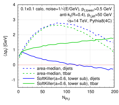
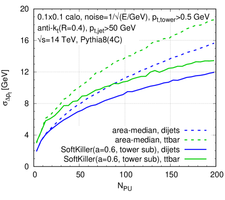
Results are shown in Fig. 12.12. The energy $E$ in each $0.1\times 0.1$ tower is taken to have Gaussian fluctuations with relative standard deviation $1/\sqrt{E/\!\,\mathrm{GeV}}$. A $p_{t}$ threshold of $0.5\,\mathrm{GeV}$ is applied to each tower after fluctuations. The SK grid spacing is set to $a=0.6$. Interestingly, with a calorimeter, the area–median method starts to have significant biases, of a couple of GeV, which can be attributed to the calorimeter’s non-linear response to soft energy. The SK biases are similar in magnitude to those in Fig. 12.5 at particle level (note, however, the need for a different choice of grid spacing $a$). The presence of a calorimeter worsens the resolution both for area–median subtraction and SK, however SK continues to perform better, even if the improvement relative to area–median subtraction is slightly smaller than for the particle-level results.

We have also investigated a direct application of the particle-level SoftKiller approach to calorimeter towers, i.e. without the subtraction in Eq. (12.3). We find that the biases were larger but still under some degree of control with an appropriate tuning of $a$, while the performance on dispersion tends to be intermediate between that of area–median subtraction and the version of SoftKiller with tower subtraction.

The above results are not intended to provide an exhaustive study of detector effects. For example, particle flow and CHS are affected by detector fluctuations, which we have ignored; purely calorimetric jet measurements are affected by the fact that calorimeter towers are of different sizes in different regions of the detector and furthermore may be combined non-trivially through topoclustering. Nevertheless, our results help illustrate that it is at least plausible that the SoftKiller approach could be adapted to a full detector environment while retaining much of its performance advantage relative to the area–median method.

12.4 Computing time

The computation time for the SoftKiller procedure has two components: the assignment of particles to patches, which is ${\cal O}\left(N\right)$, i.e. linear in the total number of particles $N$ and the determination of the median, which is ${\cal O}\left(P\ln P\right)$ where $P$ is the number of patches. The subsequent clustering is performed with a reduced number of particles, $M$, which, at high pileup is almost independent of the number of pileup particles in the original event. In this limit, the procedure is therefore expected to be dominated by the time to assign particles to patches, which is linear in $N$. This assignment is almost certainly amenable to being parallelised.

In studying the timing, we restrict our attention to particle-level events for simplicity. We believe that calorimeter-type extensions as described in section 12.3 can be coded in such a way as to obtain similar (or perhaps even better) performance.

Figure 12.13: Timings of the SoftKiller compared to standard clustering shown as a function of the number of particles in the event (left) or as a function of the number of pileup vertices (right). We compare the SoftKiller timings to the time to cluster the full event with (red) or without (green) jet area information. For the SoftKiller timings (in blue), we show individually the time spent to apply the SoftKiller to the event (dotted line), the time spent to cluster the resulting event (dashed line) and their sum (solid line). The orange dotted line corresponds to the SoftKiller timing when the particle’s rapidity and azimuth have been precomputed.

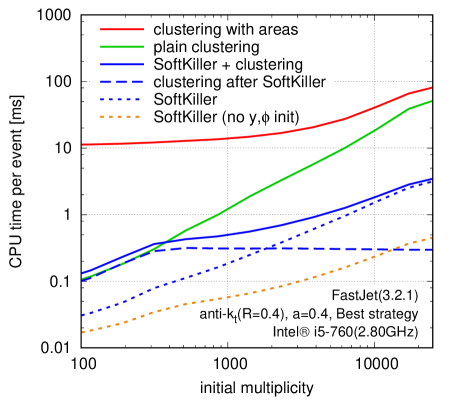
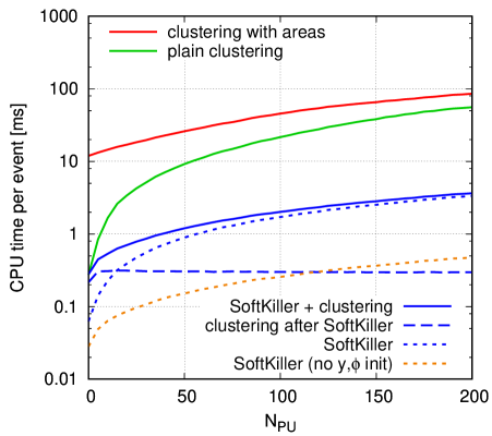
Timings are shown in Fig. 12.13 versus initial multiplicity (left) and versus the number of pileup vertices (right). Each plot shows the time needed to cluster the full event and the time to cluster the full event together with ghosts (as needed for area-based subtraction). It also shows the time to run the SoftKiller procedure, the time to cluster the resulting event, and the total time for SK plus clustering.

Overall, one sees more than one order of magnitude improvement in speed from the SK procedure, with run times per event ranging from $0.15$ to $4\,$ms as compared to $10$ to $90\,$ms for clustering with area information. At low multiplicities, the time to run SK is small compared to that needed for the subsequent clustering. As the event multiplicity increases, SK has the effect of limiting the event multiplicity to about $300$ particles, nearly independently of the level of pileup and so the clustering time saturates. However the time to run SK grows and comes to dominate over the clustering time. Asymptotically, the total event processing time then grows linearly with the level of pileup. A significant part of that time (about $130\,\text{ns}$ per particle, 75% of the run-time at high multiplicity) is taken by the determination of the particles’ rapidity and azimuth in order to assign them to a grid cell. If the particles’ rapidity and azimuth are known before applying the SoftKiller to an event (as it would be the case e.g. for calorimeter towers), the computing time to apply the SoftKiller and cluster the resulting event would be yet faster, staying below $0.5\,$ms, as indicated by the dotted orange line on Fig. 12.13.

Because of its large speed improvement, the SoftKiller method has significant potential for pileup removal at the trigger level. Since SoftKiller returns an event with fewer particles, it will have a speed performance edge also in situations where little or no time is spent in jet-area calculations (either because Voronoi areas or fast approximate implementations are used). This can be seen in Fig. 12.13 by comparing the green and the solid blue curves which stays well below $1\,\text{ms}$ even at high multiplicities.

12.5 Discussion and conclusions

The SoftKiller method appears to bring significant improvements in pileup mitigation performance, in particular as concerns the jet energy resolution, whose degradation due to pileup is reduced by $20-30\%$ relative to the area–median based methods. As an example, the performance that is obtained with area–median subtraction for 70 pileup events can be extended to 140 pileup events when using SoftKiller. This sometimes comes at the price of an increase in the biases on the jet $p_{t}$, however these biases still remain under control.

Since the method acts directly on an event’s particles, it automatically provides a correction for jet masses and jet shapes, and in all cases that we have studied brings a non-negligible improvement in resolution relative to the shape subtraction method, and also (albeit to a lesser extent) relative to the recently proposed Constituent Subtractor approach.

The method is also extremely fast, bringing nearly two orders of magnitude speed improvement over the area–median method for jet $p_{t}$’s. This can be advantageous both in time-critical applications, for example at trigger level, and in the context of fast detector simulations.

There remain a number of open questions. It would be of interest to understand, more quantitatively, why such a simple method works so well and what dictates the optimal choice of the underlying grid spacing. This might also bring insight into how to further improve the method. In particular, the method is known to have deficiencies when applied to large-$R$ ungroomed jets, which would benefit from additional study (see Section 13.2.1 for a possible solution). Finally, we have illustrated that in simple detector simulations it is possible to reproduce much of the performance improvement seen at particle level, albeit at the price of a slight adaption of the method to take into account the finite angular resolution of calorimeters. These simple studies should merely be taken as indicative, and we look forward to proper validation (and possible further adaptation) taking into account full detector effects. It would also be interesting to see a performance comparison of the SoftKiller with the recently-proposed PUPPI pileup mitigation technique [142]. We will come back to this point in our conclusions.

Chapter 13 A (rich) forest of ideas to explore

13.1 Alternative noise-reduction methods based on particle areas

Besides the SoftKiller, we have considered a series of alternative simple methods. These have only been put through a very minimal set of tests and should be considered as preliminary. Nonetheless, we find helpful to document our findings since some of the corresponding ideas can prove useful for future pileup mitigation techniques. Note that, since we were after a simple pileup-mitigation technique, all the methods presented in this Section have essentially a single free parameter. Introducing additional parameters could, at the expense of adding complexity, bring some extra flexibility and help finding improvements.

Since our goal is to provide potential alternatives for generic pileup-mitigation techniques, we shall focus mainly on the performance for the reconstruction of the jet transverse momentum. We will also consider briefly performance for the reconstruction of the jet mass. As we have already argued in the last two Chapters, jet properties like the jet mass or jet shapes are often used in the context of boosted jets, where one starts from a large-$R$ jets and applies a grooming technique. The study of the jet mass presented below should therefore merely be seen as a first basic check that our methods do not spoil critically measurements of the internal properties of jets. Additional studies like jet shapes (the equivalent of Fig. 12.9 in our SoftKiller studies) or boosted jet reconstruction (the equivalent of Fig. 12.8 in our SoftKiller studies) are left for future studies.

One avenue that we have investigated is to try to extend our area-based approach beyond jets and to apply it directly to the particles in the event. This first requires that we extend the concept of jet area to individual particles. The definition we have adopted can be seen as a particle Voronoi area: we build the Voronoi graph from all the particles in the event, withing a given rapidity acceptance, and the area associated to each particle is simply the area of its Voronoi cell, restricted to the particle’s rapidity acceptance so as to avoid infinite cells at the edges of the acceptance. The 4-vector area is then defined as a the massless 4-vector with transverse momentum given by the Voronoi (scalar) area, and rapidity and azimuthal angle of the particle.

With that definition at hand, there is an apparent straightforward way to apply the area–median subtraction directly at the level of the particles: if $A_{{\rm particle}}^{\mu}$ is the area of a given particle, one subtracts $\rho A_{{\rm particle}}^{\mu}$ from its momentum, discarding the particle altogether if its transverse momentum $p_{t}$ is smaller than $\rho A_{{\rm particle}}$. This is unfortunately over-simplified since many soft particles, corresponding to local downwards fluctuations of the pileup background would be discarded (i.e. set to a zero $p_{t}$ instead of a negative one), cutting the negative tail of pileup fluctuations while keeping the positive tail, ultimately leading to an under-subtraction of pileup.

In our preliminary studies, we have considered several particle-based pileup mitigation methods trying to avoid this under-subtraction issue. We have compared them to the area–median approach as well as to the SoftKiller approach presented in the previous Chapter.

13.1.1 List of methods

Here is the list of methods we shall discuss in this Section:

• The Area–median method serves as a robust unbiased baseline for comparison. Following our recommendations from Section 2.8 we have used a grid-based estimation of $\rho$ with a grid-size parameter of 0.55 and rapidity rescaling. We have imposed positivity constraints on the jet $p_{t}$ and mass.

• The SoftKiller method discussed at length in the previous Chapter, that removes the soft particles in the event until the estimated $\rho$ vanishes.

• A somewhat similar idea, that we shall call the Soft-Removal method in what follows, is to remove the soft particles in the event until the total (scalar) $p_{t}$ that has been eliminated reaches $f_{\text{SR}}\rho A_{\text{tot}}$, where $\rho$ is the pileup density (if rescaling is active, it is estimated at $y=0$), $A_{\text{tot}}$ is the total detector area and $f_{\text{SR}}$ an overall factor, taken as a free parameter. Taking $f_{\text{SR}}$ to 1, we should expect to over-subtract the transverse momentum of the hard jets since the unsubtracted pileup fluctuations left across the whole event would be partially compensated by the subtraction of particles from the hard jets. We shall therefore consider values of $f_{\text{SR}}$ smaller than 1 in what follows.

• A Voronoi Killer method which works, in a similar spirit as the SoftKiller, by removing the softest particles in the event until, a fraction $f_{\text{V}K}$ of the total event area, computed from the particle Voronoi area, is empty.

• Let us come back to the idea of subtracting $\rho A_{{\rm particle}}$ from each particle, setting to 0 the particles with $p_{t}<\rho A_{{\rm particle}}$. As argued above, this would leave a potentially large positive bias (i.e. an under-subtraction). This bias is expected to be proportional to the internal fluctuations of the pileup in the event, i.e. to $\sigma$. A possible solution would be to subtract, on top of $\rho A_{{\rm particle}}$ from each particle, an additional amount proportional to $\sigma\sqrt{A_{{\rm particle}}}$. We have tried 3 approaches based on this idea:

  • Voronoi Subtraction: we apply a subtraction to each of the original particle. For a particle with original transverse momentum $p_{t}$ and Voronoi area $A$, we set its subtracted transverse momentum to $\max(p_{t}-\rho A-f_{\text{VS}}\sigma\sqrt{A},0)$ where $f_{\text{VS}}$ is an adjustable parameter.

  • Voronoi Cut: the subtracted event is built by keeping the particles with $p_{t}>\rho A-f_{\text{VC}}\sigma\sqrt{A}$ (untouched) and discarding the others. $f_{\text{VC}}$ is again an adjustable parameter.

  • Voronoi Subtract&Cut: we first subtract $\rho\sqrt{A}$ from each particle in the event, discarding particles with $p_{t}<\rho\sqrt{A}$. We then remove all the particles for which the subtracted $p_{t}$ is below $f_{\text{VSC}}\sigma\sqrt{A}$, with $f_{\text{VSC}}$ an adjustable parameter. Note that this last option is somewhat reminiscent of the adaptation of the SoftKiller method to calorimeters — see Section 12.3 — and can therefore likely be applied straightforwardly in an experimental context.

There are also two other methods that we briefly investigated but were relatively rapidly abandoned since our initial findings did not give very promising results. For the sake of completeness, we introduce them here, discuss why we believe they are not efficient and quote possible options to improve them. Both methods subtract from the event a total transverse momentum of $\rho A_{\rm tot}$, with $A_{\rm tot}$ the total area of the detector. They both first subtract $\rho A_{{\rm particle}}$ from each particle, discarding the particles for which this would give a negative transverse momentum. Since we have put some of the particles to $0$ transverse momentum, the total subtracted scalar $p_{t}$ is less than $\rho A_{\rm tot}$ and an extra subtraction is needed. We then consider two possible options:

• the excess, between $\rho A_{\rm tot}$ and what has been subtracted from the initial step is subtracted uniformly over the remaining particles. We again subtract an amount proportional to their area, setting to 0 the particles for which this would give a negative $p_{t}$. The operation is repeated until a total of $\rho A_{\rm tot}$ has been subtracted. We dubbed this method Voronoi subtraction with Uniform Balance.

• alternatively, after the initial subtraction step, we successively remove the softest particle in the event until a total $p_{t}$ of $\rho A_{\rm tot}$ has been subtracted. We call this the Voronoi subtraction with Soft Balance.

In both cases, the idea here is to balance the negative part of the fluctuations, cut by the initial subtraction, with the positive part, hopefully discarded in subsequent subtractions or particle removal.

In both cases, this actually lead to a rather larger negative bias on the reconstruction of the jet $p_{t}$. We believe this is due to a reason similar to our argument in to use $f_{\text{SR}}<1$ for the Soft-Removal method. After the initial subtraction, we are essentially left with two kinds of objects: hard jets located around a few directions in the event and pileup upwards fluctuations distributed uniformly across the event. Ideally, only the pileup component need to be subtracted but in practice, both these components will be affected by the subsequent steps of the subtraction. This will lead to some upwards pileup fluctuations left uniformly across the event and an oversubtraction of the hard jets to compensate for that effect. Similarly to the Soft-Removal method, a tentative solution to that issue would be to adapt the method and only subtract a fraction $f$ of the total $\rho A_{\rm tot}$, with $f$ an adjustable parameter. We have not (yet) investigated that option.

Note also that we could have considered a third option where the amount left to subtract after the initial subtraction is balanced using the particle’s neighbours (there are actually several ways to achieve that). In practice, the hard particles in the jet would be used to compensate the negative fluctuations in the jet’s vicinity, yielding once more an over-subtraction, possibly even larger than with the other two approaches.

Finally, in a more complete study, it would be interesting to include a comparison to the ConstituentSubtractor, as well as other intra-jet methods, like an intrajet killer which would iteratively remove the softest particle in a given jet until a total $p_{t}$ of $\rho A_{\text{jet}}$ has been subtracted (see footnote 12 in Chapter 12). These methods are expected to give results very close to the area–median for the jet transverse momentum and a small improvement for the jet mass.

13.1.2 Monte-Carlo studies

Description.

As usual, we work by embedding hard events in a superposition of minimum bias events to simulate pileup. Both the signal events and the minimum bias events have been generated with Pythia 8186 with the 4C tune and, for simplicity, we have set the mass of the initial particles to zero, preserving their transverse momenta, rapidities and azimuthal angles. We keep particles up to $|y|=5$. We cluster the jets using the anti-$k_{t}$ algorithm with $R=0.4$. In the hard event, we select the jets passing a given $p_{t}$ cut that we shall vary to probe the robustness of the pileup mitigation methods, and with $|y|<4$.

We apply the various event-wide pileup subtraction techniques introduced in the previous Section to the full event — including the hard event and pileup — and for each of the original hard jets, find the most overlapping jet in that subtracted event. We then focus on the shift $\left\langle\Delta p_{t}\right\rangle$ and dispersion $\sigma_{\Delta p_{t}}$ quality figures already used several times so far, in order to assess the performance of the methods introduced above. As an additional check, we also look at the reconstruction of the jet mass by studying $\left\langle\Delta m\right\rangle$ and $\sigma_{\Delta m}$.

The parameters of our candidate pileup mitigation techniques are fixed/varied as follows. For the area–median subtraction, acting as our baseline. we use a grid-based estimation of $\rho$ with the grid-size parameter set to 0.55 and rescaling to handle the rapidity dependence. The SoftKiller size parameter is varied between 0.3 and 0.7. For the Soft Removal technique, we use the pileup density $\rho$ coming from the area–median method, calculated at $y=0$ and vary $f_{\text{SR}}$ between 0.66 and 0.76. Moving to the methods based on Voronoi areas, we calculate the particle areas up to $|y|=5$. For the Voronoi Killer, we vary $f_{\text{VK}}$ between 0.94 and 0.98. Finally, for the last three Voronoi-based methods, we compute $\rho$ and $\sigma$ independently for each particle, using the area–median technique, including the rapidity dependence. We vary $f_{\text{VC}}$ between 1.5 and 3.5, $f_{\text{VSC}}$ between 0.5 and 3, and $f_{\text{VS}}$ between 0.2 and 0.7.

Since a key element common to all these new techniques is their potentially uncontrolled biases, we want to study different processes and pileup conditions to assess the robustness of the methods. We do this by selecting a few working points. First, we work with fixed pileup conditions, taking $\mu=60$ as a default, and study a few representative cuts on the jet $p_{t}$, namely $20$, $100$ and $500$ GeV. Conversely, for a fixed jet $p_{t}$ cut of $50$ GeV, we vary the pileup conditions, choosing $\mu=30$, $60$ or $140$. This should be sufficient to give a first overview of the performance of our candidate methods when varying the two main scales in the problem: the scale of the hard jet and that of pileup.

Figure 13.1: Summary of the quality measures for various pileup mitigation methods. The average $p_{t}$ shift $\left\langle\Delta p_{t}\right\rangle$ (left panel) and the associated dispersion $\sigma_{\Delta p_{t}}$ (right panel) are plotted for $\mu=60$ and different jet $p_{t}$ cuts (20, 100 and 500 GeV respectively in red, blue and black). From bottom to top, we show the results for the area–median method, for the SoftKiller for various grid size $a$, for the SoftRemoval for different $f_{\text{SR}}$, for the Voronoi Cut, the Voronoi Subtract&Cut and the Voronoi Subtraction methods, for different $f_{\text{VC}}$, $f_{\text{VSC}}$ and $f_{\text{VS}}$, respectively. For the average shift, the dashed vertical line corresponds to the ideal situation of a zero bias. For the dispersion plot, the vertical lines correspond to the baseline obtained with the area–median subtraction method.

Figure 13.2: Same as Fig. 13.1 but this time for a sample of hard jets with $p_{t}\geq 50$ GeV and studying the sensitivity of our results w.r.t. to variations of the pileup multiplicity. Different curves correspond to $\mu=30$, $60$ and $140$ (respectively in red, blue and black).

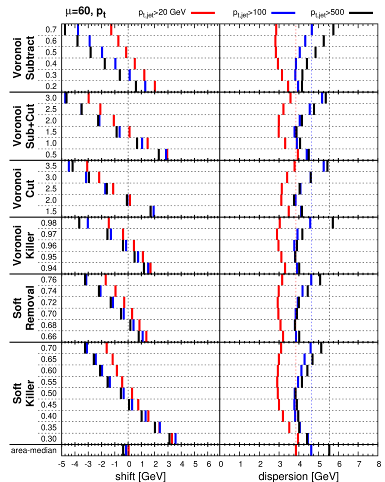
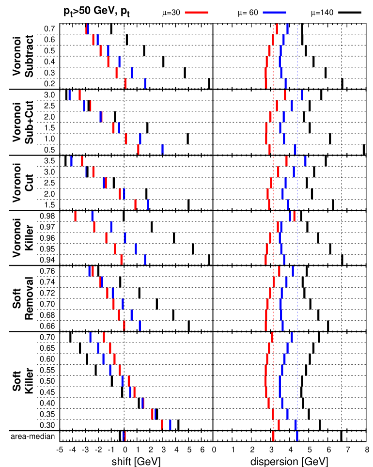
Results.

Summary plots are presented in Fig. 13.1 for the $p_{t}$ variations at fixed $\mu$ and in Fig. 13.2 for the $\mu$ dependence at fixed $p_{t}$. Overall, the message to take from these figures is that, as foreseen, one can obtain a much better resolution than with the area–median approach but at the expense of potentially large biases, strongly dependent on the adjustable parameter of the method. Below, we make more precise comments individually for each method.

Note that while the discussion focuses on the reconstruction of the most fundamental property of jets, their $p_{t}$, similar conclusions can be reached for the jet mass for which summary plots are presented in Figs. 13.3 and 13.4.

SoftKiller.

The SoftKiller with $a\approx 0.4-0.5$ shows a nice stability against both $p_{t}$ and $\mu$ variations, as well as a significant resolution improvement compared to the area–median approach. Here, we recover the results presented in details in the previous Chapter.

Soft Removal and Voronoi Killer.

These two methods show similar characteristics. For fixed pileup conditions, the subtraction bias is reasonably stable against changes in the jet $p_{t}$ with a region where it remains close to zero, but a fixed value of the adjustable parameter is unable to stay unbiased when varying the pileup conditions.

This could actually have been anticipated. If one takes, for example, the case of the Voronoi Killer, as pileup increases, the area occupied by pileup particles (resp. hard particles) increases (resp. decreases). Removing a fixed area from the event will then result in a bias increasing with pileup. A possible improvement of the method would be to adjust $f_{\text{SR}}$ or $f_{\text{VK}}$ with the pileup conditions.

It is also interesting to note that, while values of $f_{\text{VK}}$ are close to one, $f_{\text{SR}}$ is much smaller. This is likely due to the fact that we have used the value of $\rho$ estimated at $y=0$. If we take into account the rapidity profile of $\rho$, introduced in Chapter 3, we find that, for $\sqrt{s}=13$ TeV, the averaged $\rho$ for $|y|<5$ is about 83% of the $\rho(y=0)$, a value only slightly above our range for $f_{\text{SR}}$.

That said, if we consider a value of their parameter where the bias remains small, both the Soft Removal and the Voronoi Killer methods show a resolution similar to that obtained with the SoftKiller. This means that, modulo the dependence of $f_{\text{SR}}$ and $f_{\text{VK}}$ on the pileup multiplicity, which might likely be parametrised easily, these methods could give results similar to that of the SoftKiller.

Voronoi Cut, Subtract&Cut and Subtract.

Comparing the average bias observed with these three methods, one sees that, in the region where the bias is small, the Voronoi Subtract Method shows a larger dependence on $p_{t}$ and $\mu$ that the Voronoi Cut, with the mixed Voronoi Subtract&Cut method being intermediate. This indicates that a method that either keeps a particle untouched or discards it shows more stability than a method that applies a more democratic subtraction. The Voronoi Cut technique actually shows a behaviour comparable to the Soft Removal and Voronoi Killer methods discussed above with an even slightly smaller dependence on the jet $p_{t}$ and $\mu$. As long as we do not go to very large pileup multiplicities, the Voronoi Cut method with $f_{\text{VC}}\approx 2$ shows similar performance and robustness than the SoftKiller, both in terms of the average bias than in terms of dispersion, with a small advantage for the latter in terms of dispersion. Going to larger pileup multiplicities would probably necessitate a small increase of $f_{\text{VC}}$ to maintain a similar level of performance.

Figure 13.3: Same as Fig. 13.1 but this time for the jet mass rather than for the jet $p_{t}$. The left plot shows the average shift and the right plot shows the dispersion.

Figure 13.4: Same as Fig. 13.2 but this time for the jet mass rather than for the jet $p_{t}$. The left plot shows the average shift and the right plot shows the dispersion.

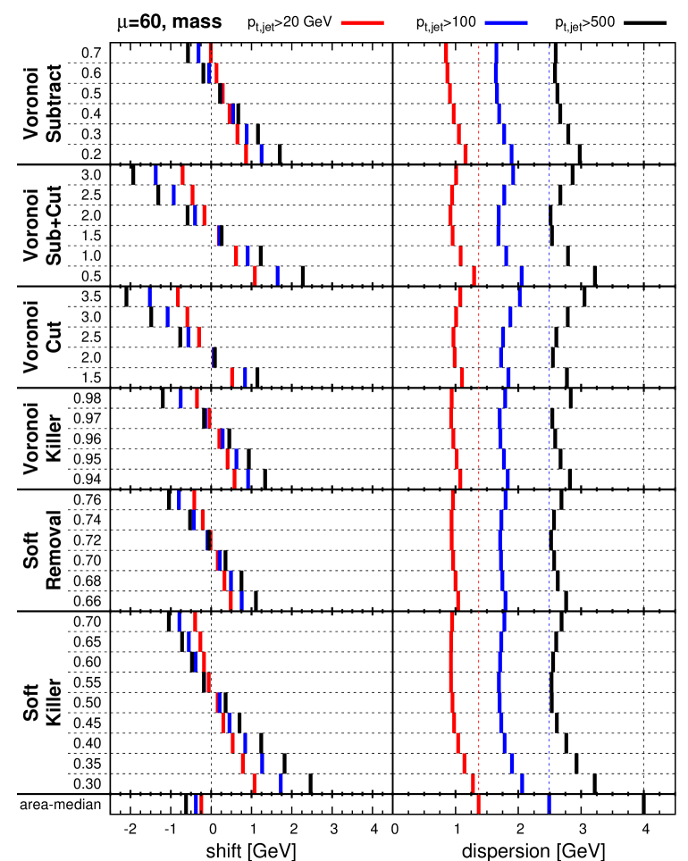
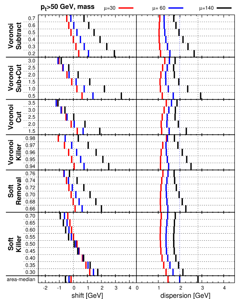
Conclusions.

In the end, all the methods show relatively similar potential resolution gains compared to the original area–median approach. Amongst the list of methods we have considered, the SoftKiller is the one showing the best stability when varying $p_{t}$ and $\mu$ and so is the one we ultimately decided to select for a deeper study. It is nevertheless interesting to notice that the Soft Removal, the Voronoi Killer and, especially, the Voronoi Cut methods, for fixed pileup conditions, all have a working point for which the average bias remains small independently of the jet $p_{t}$. Adjusting their respective free parameter with the pileup conditions would deserve further study and can potentially give performances similar to what is reached with the SoftKiller. Since the studies here remain fairly basic, e.g. they do not discuss CHS events or detector effects, the alternative approaches presented above, and the ideas they are based on, should be kept in mind for future pileup mitigation studies.

13.2 SoftKiller improvements

Studies in the previous Chapter and in the previous Section have shown that the SoftKiller is a very promising noise-reduction pileup mitigation technique. In this Section, we investigate possible improvements of the method. All the results presented here are to be considered as preliminary. We nevertheless believe that they carry useful information and might prove useful in the longer run.

In practice, we want to study two specific points. The first one is the question of the angular dependence: as we have seen in the previous Chapter, the parameter $a$ of the SoftKiller tends to depend on the jet radius $R$ used to cluster the final jets and we want to propose a possible workaround that would work independently of $R$. Note that fat jets are only one possible application of this study. The other application, potentially of broader impact, could be an improvement of the SoftKiller already at $R=0.4$ through an improved description of the angular dependence at smaller $R$.

The second question is related to our observation in Chapter 11 that “(protected) zeroing” can be useful in reducing the impact of pileup fluctuations at the expense of potentially biasing the reconstructed averaged jet properties. We want to see if zeroing can be combined with the SoftKiller for further performance gains.

13.2.1 Improved $R$ dependence

Motivation and description.

One piece of physical information that is not encoded in the SoftKiller technique is the fact that the QCD radiation from a hard jet is collinear to the jet, peaking at small angles, while pileup tends to be mostly uniform in rapidity and azimuthal angle.

In practice, this means that if one goes further away from the jet axis, particles (of a given $p_{t}$) are more likely to come from pileup. In the context of the SoftKiller, the consequence is that if we want to reconstruct jets with a larger radius, one has to increase the $p_{t}$ cut on the particles which is done in practice by increasing the size parameter $a$ of the SoftKiller.

In that context, it is natural to wonder if one can encode some form of angular dependence directly in the SoftKiller recipe to automatically allow for jet clustering with any radius. A side benefit of that approach might also be that we could also obtain a performance gain at $R=0.4$.

Implementing the physical idea that hard jets have collinear radiation while pileup is more uniform has one major difficulty: it requires some form of knowledge of where the hard jets are.

The approach we have tested is the following. For a given event, we first apply the SoftKiller with an initial grid-size parameter $a$. This corresponds to a $p_{t}$ cut $p_{t,0}$. We then cluster the event with a jet radius $R_{0}$ for which we expect the initial SoftKiller to give good performances. In our studies, we chose the anti-$k_{t}$ algorithm but this choice should not matter too much. We then keep the jets above a certain $p_{t,\rm cut}$ as our “reference hard jets”. Finally, for each particle in the event, we apply the following cut: we compute its distance to the nearest reference hard jet, $\Delta$, and discard that particle if its transverse momentum is below

$$p_{t,0}\left(\frac{{\rm max}(\Delta,R_{0})}{R_{0}}\right)^{\gamma},$$ (13.1)

where $\gamma$ is a parameter controlling the angular dependence of the cut.

Compared to the plain SoftKiller, this has three extra parameters: $R_{0}$ and $p_{t,\rm cut}$ defining the reference jets, and $\gamma$. Adding parameters allows for much more fine tuning but, at the same time, leads to a much larger phase-space to explore. A complete and thorough exploration of this phase-space goes beyond the reach of this preliminary analysis. In what follows, we shall just present a few results based on a first, very basic, exploration of the ideas we just introduced.

Testing framework.

In practice, we have used the same framework as for our SoftKiller studies. We have worked with full events (i.e. not assuming anything about charged track or neutral particles), and let the $\pi^{0}$ decay. As a first attempt to test a $R$-dependent version of the SoftKiller, we have focused on a single hard process. We have considered dijet events with a $p_{t}$ cut of 50 GeV. We have assumed $\mu=60$ in all our studies. In order to explore the parameter phasespace of the method, we have varied $a$ between 0.2 and 0.6 by steps of 0.1, $R_{0}$ between 0.1 and 0.4 by steps of 0.1, tested $\gamma=0.5,\>1$ or $2$, and $p_{t,\rm cut}=5,\>10$ or $20$ GeV. Since our main goal is to test the $R$ dependence of the method, we have studied independently $R=0.4,\>0.7$ and $1$. With no surprise, we have looked at the average shift $\Delta p_{t}$ and the associated dispersion $\sigma_{\Delta p_{t}}$ with the same matching procedure as the one used for our SoftKiller studies.

Figure 13.5: Summary of our results for the $R$-dependent extension of the SoftKiller. Each plot corresponds to different radius used to cluster jets: $R=0.4$ on the top left plot, $0.7$ on the top right plot and $R=1$ on the bottom plot. On each plot, we have plotted contours of equal shift and dispersion in the plane of the $a$ and $R_{0}$ parameters of the method. The top of the plot corresponds to the SoftKiller which only depends on $a$. The black lines indicate contours where the average bias $\Delta\equiv\left\langle\Delta p_{t}\right\rangle$ is $0,\pm 1$ or $\pm 2$ GeV. The other lines indicate contours of equal dispersion $\sigma_{\Delta p_{t}}$ where we have used the optimal dispersion for the plain SoftKiller (with $0.2\leq 1\leq 0.6$) as a reference.

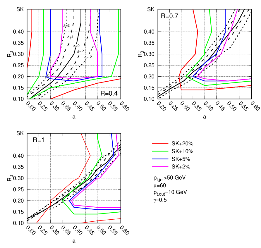
Results.

We present a summary of our findings in Fig. 13.5. For simplicity we show only results for $p_{t,\rm cut}=10$ GeV and $\gamma=0.5$. Smaller values of $p_{t,\rm cut}$ tend to give worse results and larger values only give a small improvement and could be risky for the reconstruction of jets of lower $p_{t}$. Larger $\gamma$ values show similar performance but a slightly larger dependence on the jet radius $R$.

In order to visualise the performance in a compact form, we have shown on each plot both the average shift and the dispersion, as a function of the remaining parameters, $a$ and $R_{0}$. The black lines indicate contours of equal $\left\langle\Delta p_{t}\right\rangle$ and we show them for $\left\langle\Delta p_{t}\right\rangle=0,\pm 1$ or $\pm 2$ GeV (respectively the solid, dashed and dotted lines). Ideally, we want to stay as close as possible to the solid black line which corresponds to an unbiased method. The other lines indicate contours of equal $\sigma_{\Delta p_{t}}$. For those we have first computed the optimal $\sigma_{\Delta p_{t}}$ for the plain SoftKiller (with $a$ kept within the values mentioned above, namely $0.2-0.6$) and show contours where the dispersion is larger than this minimum by $2,5,10$ or $20\%$. The results for the SoftKiller alone correspond to the values reported at the top of the plot, as a function of the parameter $a$ only.

In the end, it seems that a choice $a\approx 0.35$, $R_{0}\approx 0.2-0.25$ shows good performance across the whole range of $R$ values. However, this comes with a series of remarks and caveats.

First, we have only tested one process, one jet $p_{t}$ and one value of $\mu$. Checking the robustness of our findings for a range of processes and pileup conditions is mandatory before claiming any solid conclusion. In a similar spirit, it would be interesting to repeat the study with CHS events and, optionally, with (protected) zeroing (see the next Section). Performance for other observables like missing $E_{T}$ would also be interesting to study.

Moreover, it appears that the SoftKiller alone, with $a\approx R$ seems to give small biases and a dispersion comparable or even better than a fixed “$R$-dependent Killer”. Since larger values of $R$ are mostly used for specific purpose, one might therefore also consider applying the SoftKiller as described in Chapter 12, guaranteeing good performance for $R=0.4$ and then apply (or re-apply) the SoftKiller with a larger $a$ whenever one needs a larger $R$. In that context, it is important to note that the use of grooming techniques, inherent to the majority of the analyses involving larger $R$ values, are likely to affect the picture. This was already discussed in Section 12.2 where we noticed that a value of $a$ valid for $R=0.4$ gives good results for the groomed mass distribution of large-$R$ jets.

Finally, focusing on the results for $R=0.4$, there is a small region around $a\approx 0.35-0.4$, $R_{0}\approx 0.2-0.25$, where the bias is small and the dispersion marginally better than the SoftKiller alone. This means that this approach has a potential to bring a marginal improvement over the SoftKiller method for the standard $R=0.4$ use-case. A more definitive statement would involve a more complete study of the other parameters of the model and, in particular, an in-depth study of the robustness of the method across a range of pileup conditions and jet $p_{t}$.

Conclusions.

In the end, we find that the $R$-dependent extension of the SoftKiller method proposed here brings at best minor improvements compared to the SoftKiller alone. However, it indicates that there might be a region of our parameter space where a single working point could allow clustering with any jet radius, where a plain SoftKiller would require adapting the size parameter $a$.

There are also some signs indicating that a small improvement could be waiting around the corner, although this requires more systematic tests. In particular, we have found improvements of a few percents for $R=0.4$, compared to the SoftKiller alone. Further tests could also involve or suggest modifications of our simple central formula, Eq. (13.1). This points again to the need for studies with different processes and different pileup conditions as well as for performance tests with CHS events. Also, given similarities between the performance obtained with the SoftKiller and PUPPI (see also the summary study presented in our conclusions, Chapter 14), with the latter involving some form of angular dependence, one might wonder about the size of the gains that could be obtained from such an approach.

Finally, it would be interesting to investigate whether a toy-model approach like the one discussed in Section 5.2 could help understanding from an analytic perspective the angular dependence of the SoftKiller or its extensions.

13.2.2 Combination with (protected) zeroing

The next extension of the SoftKiller approach that we want to investigate is its combination with (protected) zeroing.

Description.

We have tested this using the following method: given a CHS event, we first apply the SoftKiller, with a size parameter $a$, on it; we then apply protected zeroing i.e. discard each of the remaining neutral particle which have no charged tracks coming from the leading vertex within a distance $R_{\rm zero}$, unless they have a transverse momentum larger than $p_{t,\rm prot}$.

We have followed the same testing scheme as for the SoftKiller in the previous Chapter and so refer to Section 12.2 for details of our simulations. The approach described above has three parameters: the grid size $a$ for the SoftKiller that we varied between 0.2 and 0.6, the zeroing radius $R_{\rm zero}$ that we varied between 0.1 and 0.3, and the protection cut $p_{t,\rm prot}$ that we fixed to 10 GeV.

Figure 13.6: Average shift, $\left\langle\Delta p_{t}\right\rangle$, obtained after applying the SoftKiller either alone (black line) or followed by a zeroing step. The shift is shown as a function of the number of pileup vertices for hard jets above 50 GeV on the left plot and as a function of the hard jet $p_{t}$ for $\mu=60$ Poisson-distributed pileup events on the right plot.

Figure 13.7: Dispersion $\sigma_{\Delta p_{t}}$ corresponding to the bias from Fig. 13.6.

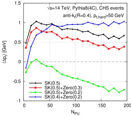
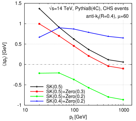
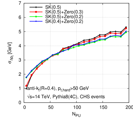
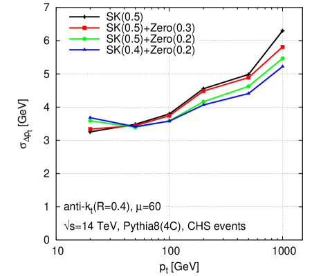
Results for the jet $p_{t}$.

On Figs. 13.6 and 13.7 we show the usual performance indicators: the average bias $\left\langle\Delta p_{t}\right\rangle$ of the reconstructed jets after pileup mitigation compared to the original hard jets, Fig. 13.6, and the associated dispersion $\sigma_{\Delta p_{t}}$, Fig. 13.7. In both cases, the results are shown as a function of the $p_{t}$ of the hard jet and as a function of the pileup multiplicity. We have selected a few representative values of $a$ and $R_{\rm zero}$ which show good performance. As expected, lowering the zeroing radius shifts the bias downwards and a first inspection seems to indicate that values of $R_{\rm zero}$ in the 0.2-0.3 range give the optimal performance. In terms of the average bias, all the combinations shown in the Figure give results of similar quality to, or marginally better than, the SoftKiller alone.

Let us now turn to the dispersion. We see that zeroing gives an improvement in extreme situations: for $a=0.4$ or $0.5$ and $R_{\rm zero}=0.2$, we gain about 15% in dispersion at large jet $p_{t}$ and around 8% at large pileup multiplicities. Unfortunately, this improvement is not present uniformly, especially at low $p_{t}$ or low pileup multiplicity where our results indicate a preference for a larger zeroing radius and only bring marginal improvement, if any, compared to the SoftKiller alone. A more careful tuning of the parameters is probably needed to reach a performance gain over the whole kinematic spectrum.

Figure 13.8: Same as Figs. 13.6 and 13.7 now for the jet mass instead of the jet $p_{t}$.

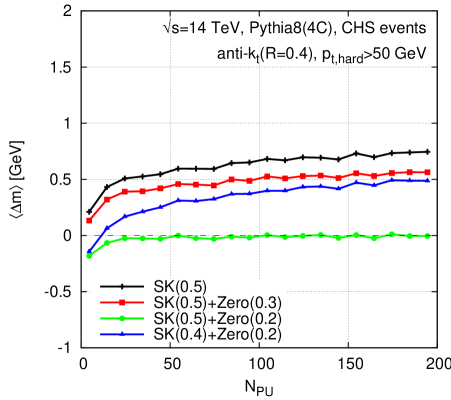
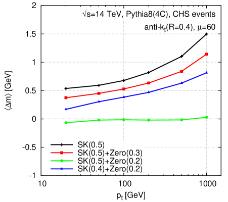
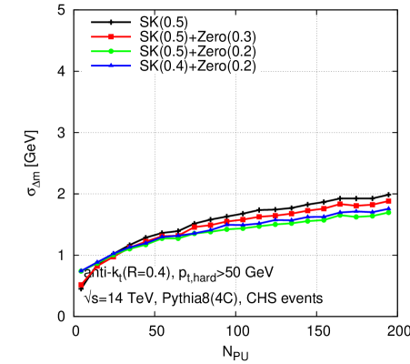
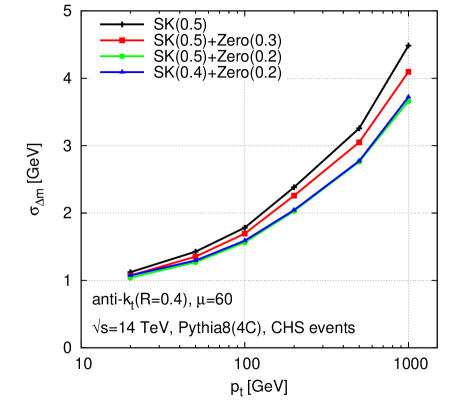
Results for the jet mass.

If one now considers the reconstruction of the jet mass instead of the jet transverse momentum, see Fig. 13.8, one sees a more interesting behaviour. First, the performance gain brought by the extra zeroing step is more manifest. Then, the combination of the SoftKiller with $a=0.5$ and zeroing with $R_{\rm zero}=0.2$ shows remarkable performance: on average the mass is reconstructed with very little bias over the whole kinematic range we have tested, and the dispersion comes out 15-20% lower than with the SoftKiller alone, without a sign of degradation at low $p_{t}$. This is coherent with our earlier observations from Chapter 11.

Conclusions.

In the end, this preliminary study indicates that (protected) zeroing can indeed improve the performance of the SoftKiller but that some degree of tuning is needed to fully optimise the method. For example, our studies show that a better performance would be obtained with a larger zeroing radius at low pileup multiplicity and low jet $p_{t}$. After that tuning is carefully done, one could expect a performance gain over the SoftKiller alone that reaches up to 15% in terms of dispersion with no significant impact on the average bias. Finally, if one focuses on the reconstruction of the jet mass instead of the jet transverse momentum, the combination of the SoftKiller with $a=0.5$ and zeroing with $R_{\rm zero}=0.2$ shows remarkable performance with nearly negligible bias and nice resolution gains. This would therefore certainly deserve more extensive studies, including tests with more busy environments like $t\bar{t}$ events and tests with a more realistic, experimental, setup.

Chapter 14 Conclusion and perspectives

Pileup, the superposition of simultaneous proton-proton collision, contaminates almost all measurements at the LHC. Being hadronic objects, jets are particularly affected by pileup and one needs to design procedures to subtract/mitigate pileup effects if one wants to reach optimal precise for measurements involving jets. This is the topic of this document. The main quantity of concerns is the widely used jet transverse momentum but we have also discussed other jet properties.

In this concluding Chapter, we will first give a brief overview of the methods that have been covered with their respective advantages and potential issues. To put that overview into perspective, we will provide a benchmark study comparing their performance in a couple of summary plots. We will then spend the last few paragraphs discussing future challenges and perspectives.

A significant fraction (the first part) of this review has concentrated on the area–median pileup subtraction method which has been used in Run I of the LHC and is still extensively in use during Run II. In Chapters 2-5, we have described how the method can be applied to a wide range of jet observables: the jet transverse momentum, the jet mass, jet shapes and even the collinear-unsafe jet fragmentation function; we have then tested its performance and studied some of its analytical properties. A summary of our recommendations for the usage of the area–median method at the LHC can be found in Section 2.8. The main benchmark of the area–median method is that it provides a robust pileup subtraction, with a very small residual bias — of order of a few 100 MeV — and a large reduction of the pileup resolution degradation effects. By “robust”, we mean that the method depends essentially on a single free parameter — the patch size used for the estimation of the pileup density — which can be chosen over a relatively wide range without affecting the overall performance of the method, independently of the process and transverse momentum scale under consideration.

One aspect that we have not discussed at all in this document is detector effects which will certainly require additional jet-calibration corrections. However, the stability of the area–median approach w.r.t. the process and kinematic dependence and w.r.t. the choice of its free parameter, indicates that the residual detector effects should also be small.

Furthermore, as we have shown in Chapter 11, the area–median method can be straightforwardly extended to Charged-Hadron-Subtracted (CHS) events, and is expected to perform slightly better than the Neutral-proportional-to-Charged (NpC) method which uses the (known) charged pileup contamination to the jet to infer their neutral contamination. This comparison could however be affected by several detector effects like the effectiveness of the CHS event reconstruction and out-of-time pileup.

In the end, the area–median pileup subtraction method can be seen as a robust and efficient reference method for pileup subtraction.

The main limitation of the area–median method is that it leaves some residual resolution degradation after the subtraction has been applied. This smearing remains small with current pileup conditions ($\mu\sim 30-50$) — see below for more quantitative information — but will increase significantly in future runs of the LHC ($\mu\sim 60-140$). This suggests that one investigates alternative pileup mitigation techniques which are less sensitive to pileup fluctuations between different points within an event. This has been investigated in the third part of our review. We have proposed a series of new methods following two main directions of though: jet grooming techniques and event-wide pileup subtraction.

Jet grooming techniques are substructure tools extensively used in the context of boosted fat jets at the LHC, and we have briefly studied this in the second part of this document. Our preliminary results for the use of jet grooming as a generic pileup mitigation tool have been presented in Chapter 10 and a discussion of the jet cleansing technique, which uses jet substructure as well, is included in Chapter 11. As far as event-wide techniques are concerned, we have made an extensive study of the SoftKiller in Chapter 13. We have also provided a brief Monte-Carlo study of a series of alternative (and still preliminary) event-wide pileup-mitigation methods, in Chapter 13, together with a few possible (also preliminary) extensions of the SoftKiller method.

These substructure-based or event-wide techniques all share similar generic patterns. As expected, they come with sometimes sizeable gains in jet resolution, especially at large pileup multiplicities. In particular, they often show a dependence on ${N_{\mathrm{PU}}}$ which grows slower that the naive $\sqrt{{N_{\mathrm{PU}}}}$ statistical behaviour. However, this gain in resolution does not come for free: in order to keep the average transverse momentum bias small, one usually needs to fine-tune the free parameters of the method, sometimes including variations of these parameters with the pileup conditions or jet energy. This contrasts with the robustness of the area–median method. Among the methods we have studies, the most stable is the SoftKiller for which a single value of the one free parameter gives acceptable biases independently of the pileup conditions, process and jet energy under consideration. The remaining average bias is around 1-2 GeV, larger than what we obtain from the area–median method but of the order of, or smaller than, the jet-energy-scale corrections applied in an experimental context.

To summarise our main findings and the many pileup mitigation techniques introduced throughout this document, we have selected a few representative methods (see below) and studied them with the framework developed for the “PileUp WorkShop” held at CERN in May 2014 [40]. Since the goal of the workshop was precisely to discuss and compare different pileup mitigation techniques using a common open-source software framework, this is perfectly suited for our summary. The code used to obtain the results presented hereafter is publicly available in the comparisons/review folder of the https://github.com/PileupWorkshop/2014PileupWorkshop GitHub [163] repository.

To avoid a proliferation of curves, we have limited the study presented here to the following representative methods:

• Area–median: this is the main method described in this review (see Part I) and should be considered as a baseline for comparisons.

• Filtering: this is meant to illustrate how jet grooming techniques can be used as generic pileup subtraction methods (see Chapter 10 for more details and other groomer options).

• Linear cleansing: this is the technique introduced in Ref. [11] and discussed in Chapter 11. It also illustrates the use of the Neutral-proportional-to-Charged method, combined with subjet techniques (and zeroing).

• SoftKiller: this method discussed in Chapter 12 is an event-wide, noise-reduction, pileup mitigation method.

• SoftKiller+Zeroing: this is the extension of the SoftKiller method proposed in Section 13.2.2, supplemented with (protected) zeroing.

• PUPPI: this is the recent method proposed in Ref. [142] and used by the CMS collaboration in Run II of the LHC.

The first 3 methods are applied individually on each jet in the full event, the last three methods are applied on the full event prior to the clustering. For all cases, we have assumed massless particles and perfect CHS events where the charged particles can be exactly reconstructed and associated either to the leading vertex or to a pileup vertex. Note that the software available from the GitHub repository includes additional options — typically, filtering with alternative parameters, area–trimming, the ConstituentSubtractor and the subtractions based on the Voronoi particle area introduced in Section 13.1 — which we will not discuss here.

The details of how the simulation and analysis are carried on are described in Appendix G, together with the parameters adopted for each of the pileup mitigation techniques. In the end, we study our usual quality measures: the average bias for the jet transverse momentum and the associated resolution. We also consider the jet mass but this should merely be considered as a cross-check that the pileup mitigation does not severely affects jet substructure measurements.

Results are plotted in Fig. 14.1 for the jet $p_{t}$ and in Fig. 14.2 for the jet mass. We have used the format advocated during the workshop which shows the dispersion versus the average bias. Each curve corresponds to a different method with the 4 points corresponding to the 4 pileup multiplicities, ${N_{\mathrm{PU}}}=30$, 60, 100 and 140 from bottom to top. Each panel of the plot corresponds to a different cut on the jet $p_{t}$ in the initial sample without pileup. We first discuss the case of the jet $p_{t}$ and move to the jet mass later on.

Figure 14.1: Performance summary for 6 representative pileup mitigation techniques. The $p_{t}$ resolution degradation due to pileup is plotted vs. the average $p_{t}$ bias for cuts on the jet $p_{t}$ ranging from 20 GeV (left panel) to 500 GeV (right panel). The 4 points on each curve corresponds to ${N_{\mathrm{PU}}}=30$, 60, 100 and 140 from bottom to top. All methods are applied on idealistic CHS events.

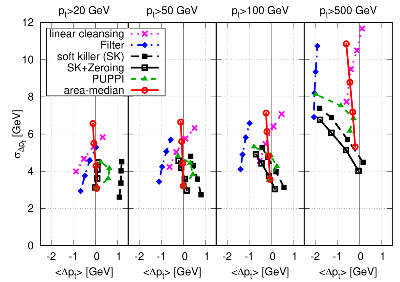
First and above all, we clearly see the stability of the area–median subtraction method (the solid red curves with empty circles): the $p_{t}$ bias remains well below 1 GeV over a wide range of pileup conditions and jet $p_{t}$. We also observe many of the other features highlighted in the first part of this document, namely that the dispersion increases like $\sqrt{{N_{\mathrm{PU}}}}$ (we have, roughly, $\sigma_{\Delta p_{t}}\approx 0.55\sqrt{{N_{\mathrm{PU}}}}$ GeV) and that the dispersion starts increasing at large $p_{t}$ (an effect associated with back-reaction).

Let us now examine to the two other jet-by-jet techniques: filtering, combined with the area–median subtraction for the subjets (the dot-dot-dashed blue line with diamond symbols), and jet cleansing, using the neutral-proportional-to-charged approach (the dotted magenta line with crosses). We see that they typically bring gains in resolution but come with a few caveats: the average bias increases and depends on either the pileup multiplicity (for cleansing) or the jet $p_{t}$ (for filtering). Furthermore, while the gain in resolution is clear at small transverse momentum and large pileup, arguably where it matters the most, the situation is less clear for large $p_{t}$ where the more robust area–median approach also gives a better resolution, or at smaller pileup multiplicity and small $p_{t}$, where only filtering shows a good performance. This illustrates the fact that, compared to the area–median method, these new techniques require an additional fine-tuning to keep the average bias under control. Some level of fine-tuning (e.g. of the subjet radius used in both filtering and jet cleansing) with ${N_{\mathrm{PU}}}$ and $p_{t}$ could also lead to a more systematic improvement in jet resolution. Note also that it would be interesting to study a combination of filtering with (protected) zeroing since this has shown performance gains with cleansing.

Finally, let us consider the 3 event-wide techniques we have included in our study: the SoftKiller alone (the long-dashed black line with filled squares) or supplemented with (protected) zeroing (the solid black line with empty squares) and PUPPI (the short-dashed green line with triangles). In terms of the average bias, we see the same trend as with the subjet techniques: a fine-tuning of the free parameters of the method is necessary to keep the bias under reasonable control, reasonable here meaning around 1-2 GeV with some residual dependence on the jet transverse momentum and the pileup conditions. Such a bias can be considered as acceptable since it remains comparable to jet energy scale corrections one would anyway have to apply in an experimental context. Furthermore, the three event-wide approaches show substantial resolution gains, especially at large pileup multiplicities, with only small differences between the methods. At low $p_{t}$, PUPPI and SoftKiller combined with zeroing behave very similarly with the SoftKiller alone showing a larger bias but a slightly better resolution for ${N_{\mathrm{PU}}}\sim 30-60$. Moving to intermediate and large $p_{t}$, the SoftKiller supplemented with zeroing seems to perform slightly better than the other two methods. It would be definitely interesting to see how this comparison behaves in a more realistic experimental context.

Note that it is worth comparing our numbers obtained for the resolution, to the CMS detector performance for the jet energy resolution [164] using particle flow [162] and CHS events. With almost no pileup ($\mu<10$), CMS reports a jet energy resolution around 3.2 GeV for 20 GeV jets, growing to $\sim 5.5$ GeV for 50 GeV jets and $\sim 10$ GeV for 100 GeV jets. This indicates, as expected, that pileup affects more low and intermediate-$p_{t}$ jets than high-$p_{t}$ jets. For 20 GeV jets, a pileup resolution degradation of 4 GeV would give about a 50% degradation in jet energy resolution, which is about what is obtained with current (end of 2016) pileup conditions. For larger pileup multiplicities, fig. 14.1 clearly points in the direction of using the new event-wide mitigation techniques, like the SoftKiller and its possible improvements, or PUPPI. For those techniques the resolution degradation is much less dramatic. Whether this can be further improved or not remains however an open question.

Turning briefly to the jet mass, Fig. 14.2, we see roughly the same pattern as for the jet $p_{t}$, although the resolution gain is larger in the case of the jet mass. In particular, it can already be seen for filtering and cleansing which use subjets, and the combination of SoftKiller and protected zeroing shows a very good performance in terms of resolution with a remarkably small average bias.

Figure 14.2: Same as Fig. 14.1, now for the jet mass instead of the jet $p_{t}$.

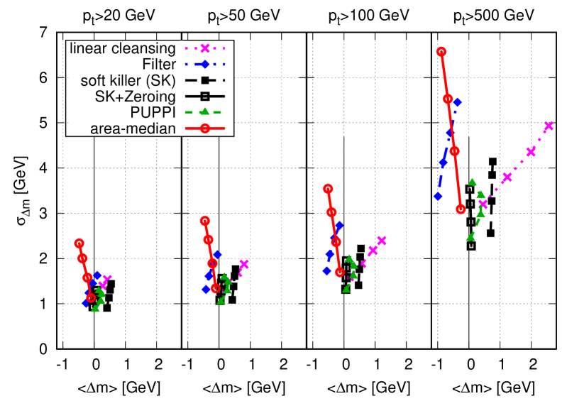
This summary study illustrates the main points developed in this document: we see that the area–median does an excellent job at providing a robust method with very small bias and process dependence, and new techniques, especially those based on event-wide subtractions, have a potential for significant resolution improvements in the coming runs of the LHC, at the expense of requiring a fine-tuning of their free parameters and a potentially more involved jet calibration.

We will now conclude with a few last generic remarks and open questions for future investigations.

First, a brief comment about speed: jet clustering (including pileup mitigation) is one of the most computer-expensive tasks in the reconstruction of an event, together with the reconstruction of charged tracks. The fast implementation of sequential algorithms provided by FastJet was clearly a step forwards in that context and recent releases of FastJet brought valuable additional gains in speed. With the increasing LHC luminosity, one might wonder if further gains can be found. In that context, one has to highlight that the SoftKiller can be implement so at to run extremely fast (see Section 12.4). Given the results of our summary study above, one might wonder if the extension of SoftKiller with protected zeroing is also amenable to such a fast implementation?

Additionally, the many discussions throughout this report has focused essentially on the impact of pileup on jets. This is the most common application but is far from the only one: pileup affects the reconstruction of all objects in a hadronic collider. The typical other examples are lepton/photon isolation and missing transverse energy (MET) reconstruction. These observables are however more dependent on the details of the detectors and hence more delicate to address using Monte Carlo studies. A few elements in this document point in the direction that a good reconstruction of MET should be more aggressive that what is used for jets. For example, in the case of an area–median-like approach, one should typically consider an extra pileup subtraction to remove the potentially large positive bias from positive fluctuations of the pileup density. Similarly, our SoftKiller studies require a larger grid-size parameter $a$ (and hence a larger associated $p_{t}$ cut) when the jet radius increases. However, other indices suggest a less aggressive pileup mitigation for MET reconstruction. For example, with an ideal, fully hermetic detector, energy-momentum conservation would guarantee a good reconstruction of MET even without any pileup mitigation.

More generally, we have (almost) not addressed detector effects and have instead tried to concentrate on more analytic aspects of pileup mitigation (see the remarks below). Most definitely, any pileup mitigation technique has to be validated in an experimental context but I believe that it is preferable to leave that delicate task directly to members of the experimental collaborations which are more aware of the associated subtle technical details. In that viewpoint, tests based on Monte Carlo simulations should serve as a solid indication that a method is worth of further investigations. Active discussions between the LHC phenomenologists and the experimental collaborations can only be beneficial to address potential issues or technical details and to ultimately aim at efficient pileup mitigation techniques.

Let me finish this final Chapter with a few remarks on how analytic insight and calculations have been, and can still be, useful in the context of pileup mitigation, a topic that might seem purely experimental at first sight. First, we have seen repeatedly in this document that simple analytic descriptions of the pileup energy deposit often allow one to understand the main features observed in Monte Carlo simulations. Already using a Gaussian approximation is sufficient to grasp many aspects of how pileup affects jets and how the area–median subtraction behaves. It is also interesting to point out that, as pileup multiplicity increases, the Gaussian approximation becomes valid over a increasingly wide range of scales. This fundamental understanding is key to gain confidence in a pileup mitigation method. Identifying physical properties of existing pileup mitigation techniques through a simple analytic understanding can also be of potential help towards developing new, more efficient, methods.

On a different level, analytic developments presented in this review are intimately connected to other aspects of perturbative QCD. The area–median method introduces a new property of jets, namely their area, and we have seen in Chapter 5 that many analytic results can be derived for that quantity. Our results show rich structures which can be of potential interest for tests of Monte Carlo event generators. Since jet areas are intrinsically non-perturbative quantities, sensitive to soft particles, this is naturally true for the tuning of non-perturbative models of the Underlying Event. Additionally, we have seen that the dependence of the jet area on the jet $p_{t}$ can be understood from perturbative QCD. This could provide constraints on parton showers, and we have indeed seen some differences between different generators and shower models included in our studies. Even on a more technical ground, jet areas show fundamental properties that are still to be understood. This includes for example the distribution of pure-ghost jets (see Fig. 5.4) or the appearance of fractal jet boundaries (see Section 5.1.2.4).

Another situation where analytic calculations are important is the case of jet grooming, discussed briefly in Chapter 8. This is intimately related to the understanding of jet substructure from first-principles in QCD, an area that is still fairly young and has received quite a lot of interest over the past couple of years.

More generally, I believe that a combination of perturbative QCD understanding of jets and modelling of the properties of pileup — either using a simple Gaussian approximation, more refined toy models like those described in Section 5.2, or directly measurements from data — is one of the most promising way towards developing and controlling new pileup mitigation techniques.

As for jet areas and jet substructure, a first-principles understanding comes with two advantages. First, it can provide a simple picture to explain the main features of a given pileup mitigation method. More importantly, it could help understanding from basic principles how the average bias and resolution behaves when varying pileup conditions, the jet transverse momentum, the jet radius, or the parameters of a given pileup mitigation technique. This is somehow similar to the calculation of the anomalous dimension for jet areas and to our analytic discussions of jet grooming, In a context where the tendency is to develop event-wide pileup mitigation methods with noise reduction, such a first-principles understanding might be the key to keep under control the potentially large biases inherent to these methods. It could therefore largely reduce the need for fine-tuning and improve both the effectiveness and the robustness of future pileup mitigation techniques.

Acknowledgements

The body of work presented here is the result of many scientific collaborations and human interactions. Elements of this document date back from the early days of 2007 when I started to be involved in jet physics. Trying to look back, it seems to me like the path between then and now has been paved with a pile of positive encounters which have left a trace on who I am today.

First and above all, a very special thanks goes to Matteo Cacciari and Gavin Salam for a decade worth of fruitful team work. I hardly see how any of this could have existed without them. It has been, and still is, a great adventure during which I have learned a lot about physics and human aspects of a longstanding collaboration. I can only look forwards to more of this.

There are many other scientists who contributed to various degrees in some of the results presented here. This includes direct collaborators like Jihun Kim, Paloma Quiroga-Arias, Juan Rojo, Jesse Thaler, Simone Marzani, Andrew Larkoski and Souvik Dutta. They each carry a part of my memories associated with the work detailed below.

This list can be extended to a long series of people I have interacted with and talked to over the same period. This obviously includes colleagues at the IPhT, LPTHE, BNL and CERN but also countless people met in conferences, seminars, visits and schools. This includes in particular Nestor Armesto, Mrinal Dasgupta, David Krohn, Matthew Low, Michelangelo Mangano, Guilherme Milhano, Carlos Salgado, Sebastian Sapeta, Matthew Schwartz, Liantao Wang and Urs Wiedemann.

Next, even though the title of this document might suggest otherwise, I have greatly benefited from many interactions with the experimental colleagues: Helen Caines, David d’Enterria, Guenther Dissertori, Phil Harris, Peter Jacobs, David Miller, Filip Moortgat, Matt Nguyen, Matteusz Ploskon, Sal Rappoccio, Guenther Roland, Christophe Royon, Sevil Salur, Ariel Schwartzman, and, last but not least, Peter Loch from whom I have learned a great deal of experimental details in lively discussions during the Les-Houches workshop series and beyond.

There are 6 other scientists who deserve a special thanks, namely Fawzi Boudjema, Jon Butterworth, Abdelhak Djouadi, Marumi Kado, Samuel Wallon and Bryan Webber, who have accepted to review this document, initially written as a French habilitation thesis, as members of the jury. I know it is a heavy task and I hope they nevertheless managed to get something out of this lengthy document. In a similar spirit, I wish to thank the anonymous Physics Reports referee for the careful reading of the manuscript and the helpful comments.

As I said above this is both a scientific and a human story. All this work has been built on a firm ground of family and friends. Their continuous presence is the crucial part which has allowed me to enjoy life at least as much as I have enjoyed the science. This includes a special thought for a few close family members who have sadly passed away during the past ten (or fifteen) years. On a much brighter side, I am infinitely grateful (and many of you should probably be as well) to Emilie who has lived with me through all of this journey, for example supporting my work at odd times and in odd places. My final thanks go to Thiago, Neil and Alana, together with apologies for having more than once traded playing games with them for research. I have no doubt that the years to come will bring many moments of great fun with all of them.

Over the years, this work has been supported by many institutions (the LPTHE at the University Pierre et Marie Curie, the Brookhaven National Laboratory, CERN, the French CNRS and the IPhT at the CEA Saclay) and several grants (Contract No. DE-AC02-98CH10886 with the U.S. Department of Energy, the French ANR grant Jets4LHC under number ANR-10-CEXC-009-01, the ERC advanced grant Higgs@LHC and the French ANR grant OptimalJets under number ANR-15-CE31-0016). I thank them all for their support.

Appendix A Jet algorithms and definitions

Throughout this document we have mostly considered four jet algorithms: anti-$k_{t}$ [41], $k_{t}$ [45, 46], Cambridge/Aachen [49, 50] and SISCone [122]. We provide here a very brief description of how they work.

A.1 Recombination algorithms

The anti-$k_{t}$, $k_{t}$, and Cambridge/Aachen algorithms cluster the jets via successive recombinations. Then can all be seen as special cases of the generalised-$k_{t}$ algorithm [41].

One first introduces a distance $d_{ij}$ between each pair of particles and a beam distance $d_{iB}$ for each particle:

$$d_{ij}=\text{min}(k_{ti}^{2p},k_{tj}^{2p})\frac{\Delta y_{ij}^{2}+\Delta\phi_{ij}^{2}}{R^{2}}\,,\qquad d_{iB}=k_{ti}^{2p}\,.$$ (A.1)

The free parameters are $R$, the jet radius, and $p$. The anti-$k_{t}$, $k_{t}$, and Cambridge/Aachen algorithms respectively correspond to $p=-1$, $1$ and $0$.

One then iteratively repeat the following procedure until no particles are left: at each step, the smallest distance is computed. If it involves a pair of particles, they are recombined using a $E$-scheme sum of four-momenta (i.e. direct addition of the four-momenta), otherwise the particle is “clustered with the beam”, i.e. called a jet.

A.2 The SISCone algorithm

The SISCone jet algorithm is an infrared- and collinear-safe implementation of a modern cone algorithm. It first finds all stable cones of radius $R$, a stable cone being a circle in the $(y,\phi)$ plane such that the $E$-scheme sum of the momenta inside the cone points in the same direction as the centre of the cone. It then runs a Tevatron run II type [123] split–merge procedure to deal with overlapping stable cones. The stable cones are ordered in $\tilde{p}_{t}$, the scalar sum of the $p_{t}$ of a cone’s constituents, to produce the initial list of protojets. One takes the hardest protojet and finds the next hardest one that overlaps with it (its scaled transverse momentum being $\tilde{p}_{t,j}$). If the shared $\tilde{p}_{t}$ is larger than $f\tilde{p}_{t,j}$ ($f$ is the split–merge overlap threshold parameter for the algorithm), they are merged, otherwise, the common particles are attributed to the protojet with the closer centre. If no overlaps are found, the protojet is added to the list of jets and removed from the list of protojets. This is repeated until no protojets remain.

Appendix B Representations of the jet fragmentation

A jet fragmentation function can be defined as the distribution $dN_{h}/dz$ of the momentum fraction $z=p_{t,h}/(\sum_{i\in\text{jet}}p_{t,i})$, of hadrons in the jet, where $p_{t,h}$ is the transverse momentum of the hadron.

Figure B.1: Jet fragmentation functions (versus $z$ and $\xi$) and moments (versus $N$) in $pp$ collisions at the LHC ($\sqrt{s_{NN}}=2.76$ TeV), obtained without quenching (Pythia 6), and with quenching (Pyquen).

The left-most plot of Figure B.1 shows the typical shape of the $z$ distribution (normalised to the total number of jets $N_{\text{jet}}$), given for anti-$k_{t}$ ($R=0.4$) jets with $p_{t}>100\,\mathrm{GeV}$ in $pp$ with $\sqrt{s}=2.76\,\mathrm{TeV}$. The middle plot shows identical information, represented as a differential distribution in $\xi=\ln 1/z$. The $z$ representation helps visualise the hard region of the FF, while $\xi$ devotes more space to the soft part. Two curves are shown: the solid blue, labelled “Pythia 6”, is a $pp$ reference curve obtained from Pythia 6.425 with its virtuality-ordered shower; the dashed green was obtained with the Pyquen program [81, 94], which modifies Pythia showering so as to simulate quenching. We have used it with settings corresponding to $0-10\%$ centrality. Its effect on the FF is of the same order of magnitude as the effects seen experimentally [165, 166]. Independently of any question of whether it correctly models the underlying physics, Pyquen provides therefore a useful reference when establishing whether FFs are being reconstructed with sufficient accuracy by some given procedure.

The right-most plot of Fig. B.1 shows moments of the fragmentation functions. The $N^{\text{th}}$ moment, $M_{N}$, of the fragmentation function is given by the integral

$$M_{N}=\frac{1}{N_{\text{jet}}}\int_{0}^{1}z^{N}\,\frac{dN_{h}}{dz}\,dz=\frac{1}{N_{\text{jet}}}\int_{0}^{\infty}e^{-N\xi}\,\frac{dN_{h}}{d\xi}\,d\xi\,.$$ (B.1)

In practice, the moments for a single jet can be calculated as

$$M_{N}^{\text{jet}}=\frac{\sum_{i\in{\text{jet}}}p_{t,i}^{N}}{(\sum_{i\in\text{jet}}p_{t,i})^{N}}\,,$$ (B.2)

where the sum runs over all the jet’s constituents. The results can then be averaged over many jets, so that $M_{N}=\left\langle\smash{M_{N}^{\text{jet}}}\right\rangle_{\text{jets}}$. Obviously, $M_{0}$ represents the average particle multiplicity in a jet, and $M_{1}$ is equal to one by virtue of momentum conservation, provided one measures all hadrons, as we assume here (taking $\pi_{0}$’s to be stable). If instead only charged tracks are used in the numerator, then it is clear that $M_{1}$ will be significantly below $1$. There is another value of $N$ that is of special interest: given a jet spectrum $d\sigma_{\text{jet}}/dp_{t}$ that falls as $p_{t}^{-n}$, the ratio of the inclusive hadron spectrum and inclusive jet spectrum is given by $M_{n-1}$. Thus, $M_{n-1}^{\text{AA}}/M_{n-1}^{\text{pp}}$ corresponds to the ratio of (charged-)hadron and jet $R_{\text{AA}}$ values (in the approximation that $n$ is exactly independent of $p_{t}$),

$$\frac{M_{n-1}^{\text{AA}}}{M_{n-1}^{\text{pp}}}=\frac{R_{\text{AA}}^{\text{h}}}{R_{\text{AA}}^{\text{jet}}}\,.$$ (B.3)

For $p_{t}$ in the range $100-200\,\mathrm{GeV}$, at $\sqrt{s}_{NN}=2.76\,\mathrm{TeV}$, the relevant $n$ value has some dependence on $p_{t}$ and is in the range $n=6-7$, corresponding to $N=5-6$.

Figure B.2: Representation of the $\xi$ values that contribute dominantly to the $M_{N}$ integral for a given $N$, shown as a function of $N$. Shown for the Pythia 6 results and cuts of Fig. B.1.

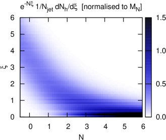
In representing the moments in figure B.1(right), we include a factor $((N+1)/2)^{4}$, which allows a broad range of $N$ values to be shown on a linear vertical scale. The same features visible in the plots versus $z$ and $\xi$ are visible versus $N$ too, for example that Pyquen leads to higher multiplicities than Pythia at small $N$ (corresponding to $z<0.05$ or $\xi>3$) and large $N$ ($z>0.5$, $\xi<0.7$), and a slightly reduced multiplicity at intermediate $N$ ($z\sim 0.2$, $\xi\sim 1.5$).

To help understand the quantitative relationship between $N$ and $\xi$, one may examine figure B.2, a colour-map that shows as a function of $N$ the contribution to the $M_{N}$ moment from each $\xi$ value. It shows clearly how large $\xi$ values dominate for low $N$ (and vice-versa). This $\xi,N$ relationship depends to some extent on the shape of the fragmentation function and it is given for the same Pythia 6 fragmentation function that was used in Fig. B.1.

Appendix C The correlation coefficient as a quality measure

In this appendix, we discuss some characteristics of correlation coefficients that affect their appropriateness as generic quality measures for pileup studies.

Suppose we have an observable $v$. Define

$$\Delta v=v^{\text{sub}}-v^{\text{hard}}\,,$$ (C.1)

to be the difference, in a given event, between the pileup-subtracted observable and the original “hard” value without pileup. Two widely used quality measures for the performance of pileup subtraction are the average offset of $v$, $\langle\Delta v\rangle$ and the standard deviation of $\Delta v$, which we write as $\sigma_{\Delta v}$. One might think there is a drawback in keeping track of two measures, in part because it is not clear which of the two is more important. It is our view that the two measures provide complementary information: if one aims to reduce systematic errors in a precision measurement then a near-zero average offset may be the most important requirement, so as not to be plagued by issues related to the systematic error on the offset. In a search for a resonance peak, then one aims for the narrowest peak, and so the smallest possible standard deviation.

Another quality measure, advocated for example in [11], is the correlation coefficient between $v^{\text{sub}}$ and $v^{\text{hard}}$. This has the apparent simplifying advantage of providing just a single quality measure. However, it comes at the expense of masking potentially important information: for example, a method with a large offset and one with no offset will give identical correlation coefficients, because the correlation coefficient is simply insensitive to (constant) offsets.

Figure C.1: Left: scatter plot of the dijet mass after addition of an average of $100$ pileup events and area–median subtraction (in CHS events) versus the dijet mass in the original hard event. The hard dijet sample and the analysis are as described in appendix E, with a jet radius of $R=1$. The right-hand plot is identical except for the following additional condition on the hard event: $450<m_{jj}<550\,\mathrm{GeV}$. Note the lower correlation coefficient, even though the lower $\sigma_{\Delta m_{jj}}$ suggests better typical subtraction in this specific mass bin.

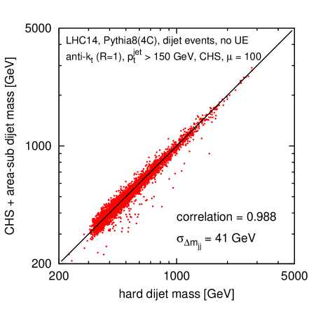
The correlation coefficient has a second, more fundamental flaw, as illustrated in Fig. C.1. On the left, one has a scatter plot of the dijet mass in PU-subtracted events versus the dijet mass in the corresponding hard events, as obtained in an inclusive jet sample. There is a broad spread of dijet masses, much wider than the standard deviation of $\Delta m_{jj}$, and so the correlation coefficient comes out very high, $c=0.988$. Now suppose we are interested in reconstructing resonances with a mass near $500\,\mathrm{GeV}$, and so consider only hard events in which $450<m_{jj}<550\,\mathrm{GeV}$ (right-hand plot). Now the correlation coefficient is $0.59$, i.e. much worse. This does not reflect a much worse subtraction: actually, $\sigma_{\Delta m_{jj}}$ is better (lower) in the sample with a limited $m_{jj}$ window, $\sigma_{\Delta m_{jj}}=34\,\mathrm{GeV}$, than in the full sample, $\sigma_{\Delta m_{jj}}=41\,\mathrm{GeV}$. The reason for the puzzling decrease in the correlation coefficient is that the dispersion of $m_{jj}$ is much smaller than before, and so the dispersion of $\Delta m_{jj}$ is now comparable to that of $m_{jj}$: it is this, and not an actual degradation of performance, that leads to a small correlation.

This can be understood quantitatively in a simple model with two variables: let $v^{\text{hard}}$ have a standard deviation of $\sigma_{v,\text{hard}}$, and for a given $v^{\text{hard}}$ let $v^{\text{sub}}$ be distributed with a mean value equal to $v^{\text{hard}}$ (plus an optional constant offset) and a standard deviation of $\sigma_{\Delta v}$ (independent of $v^{\text{hard}}$). Then the correlation coefficient of $v^{\text{hard}}$ and $v^{\text{sub}}$ is

$$c=\frac{\sigma_{v,\text{hard}}}{\sqrt{(\sigma_{v,\text{hard}})^{2}+\sigma_{\Delta v}^{2}}}\,,$$ (C.2)

i.e. it tends to zero for $\sigma_{v,\text{hard}}\ll\sigma_{\Delta v}$ and to $1$ for large $\sigma_{v,\text{hard}}\gg\sigma_{\Delta v}$, in accord with the qualitative behaviour seen in Fig. C.1. The discussion becomes more involved if $\langle v^{\text{sub}}\rangle$ has a more complicated dependence on $v^{\text{hard}}$ or if $\sigma_{\Delta v}$ itself depends on $v^{\text{hard}}$ (as is actually the case for several practical applications, like dijet mass studies).

The main conclusion from this appendix is that correlation coefficients mix together information about the quality of pileup mitigation and information about the hard event sample being studied. It is then highly non-trivial to extract just the information about the pileup subtraction. This can lead to considerable confusion, for example, when evaluating the robustness of a method against the choice of hard sample. Overall therefore, it is our recommendation that one consider direct measures of the dispersion introduced by the pileup and subtraction and not correlation coefficients. In cases with severely non-Gaussian tails in the $\Delta v$ distributions it can additionally be useful to consider quality measures more directly related to the peak structure of the $\Delta v$ distribution.

Appendix D More analytics results for jet areas

D.1 Transition from one-particle jet to soft jet.

Having observed in Chapter 5 the different properties of the area of pure ghost jets and jets containing a hard particle, one may wonder what happens to the area of a jet containing a “trigger” particle whose transverse momentum $p_{t}$ is progressively reduced, until it becomes much smaller (ultrasoft) than the momentum scale of a soft background, $\pi R^{2}\rho$.

Figure D.1: Area of the jet containing a trigger particle when it is immersed in a bath of soft particles with transverse momentum momentum density $\rho$; shown as a function of the trigger particle transverse momentum.

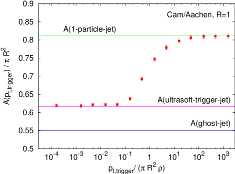
Figure D.1 show our findings for the areas obtained with the Cambridge/Aachen algorithm. As one expects, that there are two asymptotic regions. At large $p_{t}$, the area tends to that of a jet with an infinitely hard particle, Eq. (5.22). At small $p_{t}$, it tends not to the pure ghost jet area, Eq. (5.25), as one might naively expect, but rather to a value which can be predicted as

$$A(\text{ultrasoft-trigger-jet})={{\int dA\,A^{2}\,dN/dA}\over{\int dA\,A\,dN/dA}}\,,$$ (D.1)

where $dN/dA$ is the distribution of the number of pure ghost jets with a given area, and corresponds to the solid curves depicted in figure 5.4. This equation can be understood in the following way: when the momentum of the trigger particle becomes negligible compared to that of the soft background, it does not influence the size of its own jet. However, the likelihood of the trigger particle being found in a soft-background jet is proportional to that soft-background jet’s area and one gets an extra factor of $A$ in the integrand of the numerator of Eq. (D.1). One is able to use the pure-ghost-jet area distribution in Eq. (D.1), because it coincides with that of soft background jets.

Figure D.1 helps to illustrate the point that a diffuse background of particles such as pileup (represented here by the ghosts) provides an effective cutoff scale, below which a particle will not have any effect on the jet’s area. Numerically, the effective cutoff does indeed coincide with the soft-transverse momentum scale $\pi R^{2}\rho$.

D.2 Fluctuations of the active area

Finally, we derive the results Eqs. (5.37)–(5.39) for the fluctuation coefficient $S^{2}_{\text{JA},R}$ in the case of active areas. This is slightly more technical than for passive areas as we also have to deal with averages over ghosts distributions. Let us briefly recall our notation: $\left\langle\cdots\right\rangle$ represents an average over perturbative emission, while $\left\langle\cdots\right\rangle_{g}$ is an average over ghosts ensembles. When a quantity is evaluated for a specific ghost ensemble $\{g_{i}\}$, we will explicitly state so with notation of the form $A_{\text{JA},R}(\cdots\!\,|\,\{g_{i}\})$. Otherwise, we have the implicit notation that a quantity specified without any mention of ghosts, such as $A_{\text{JA},R}(0)$ is already averaged over ghost ensembles.

At order $\alpha_{s}$, the mean active area can then be written (using $A_{\text{JA},R}(\Delta=0)=A_{\text{JA},R}(\text{one particle})$)

$$\left\langle A_{\text{JA},R}\right\rangle \equiv \left\langle\left\langle A_{\text{JA},R}(\cdots\!\,|\,\{g_{i}\})\right\rangle\right\rangle_{g}$$ (D.2)

$$\simeq \left\langle A_{\text{JA},R}(0\,|\,\{g_{i}\})+\int dP\,[A_{\text{JA},R}(\Delta\,|\,\{g_{i}\})-A_{\text{JA},R}(0\,|\,\{g_{i}\})]\right\rangle_{\!g}$$ (D.3)

$$\simeq A_{\text{JA},R}(0)+D_{\text{JA},R}\frac{C_{1}}{\pi b_{0}}\log\left(\frac{\alpha_{s}(Q_{0})}{\alpha_{s}(Rp_{t,1})}\right),$$ (D.4)

with

$$D_{\text{JA},R}=\int\frac{d\Delta}{\Delta}\,(\left\langle A_{\text{JA},R}(\Delta\,|\,\{g_{i}\})\right\rangle_{g}-\left\langle A_{\text{JA},R}(0\,|\,\{g_{i}\})\right\rangle_{g}).$$ (D.5)

Here, we have taken into account both the corrections due to the radiation of a soft particle and the average over the distribution of the ghosts. Note that we have used the shorthand $dP$ to represent Eq. (5.9), $dP/(dp_{t2}d\Delta)$, times $dp_{t2}d\Delta$, and that “$\cdots$” in Eq. (D.2) represents all possible perturbative states.

For the corresponding fluctuations, the derivation goes along the same line

$$\left\langle\Sigma^{2}_{\text{JA},R}\right\rangle = \left\langle\left\langle A^{2}_{\text{JA},R}(\cdots\!\,|\,\{g_{i}\})\right\rangle\right\rangle_{g}-\left\langle A_{\text{JA},R}\right\rangle^{2}$$ (D.7)

$$= \left\langle A^{2}_{\text{JA},R}(0\,|\,\{g_{i}\})+\int dP\,[A^{2}_{\text{JA},R}(\Delta\,|\,\{g_{i}\})-A^{2}_{\text{JA},R}(0\,|\,\{g_{i}\})]\right\rangle_{\!g}$$

$$-\left\langle A_{\text{JA},R}(0\,|\,\{g_{i}\})+\int dP\,[A_{\text{JA},R}(\Delta\,|\,\{g_{i}\})-A_{\text{JA},R}(0\,|\,\{g_{i}\})]\right\rangle_{\!g}^{\!2}.$$

Neglecting the terms proportional to $\alpha_{s}^{2}$, we can write $\left\langle\Sigma^{2}_{\text{JA},R}\right\rangle=\Sigma^{2}_{\text{JA},R}(0)+\left\langle\Delta\Sigma^{2}_{\text{JA},R}\right\rangle$, where

$$\Sigma^{2}_{\text{JA},R}(\Delta)=\left\langle A^{2}_{\text{JA},R}(\Delta\,|\,\{g_{i}\})\right\rangle_{g}-\left\langle A_{\text{JA},R}(\Delta\,|\,\{g_{i}\})\right\rangle_{g}^{2}\,,$$ (D.8)

which for $\Delta=0$ is the leading order result. We can also write

$$\left\langle\Delta\Sigma^{2}_{\text{JA},R}\right\rangle=S^{2}_{\text{JA},R}\frac{C_{1}}{\pi b_{0}}\log\left(\frac{\alpha_{s}(Q_{0})}{\alpha_{s}(Rp_{t,1})}\right).$$ (D.9)

Using straightforward algebra one obtains

$$S^{2}_{\text{JA},R} = \int\frac{d\Delta}{\Delta}\,\left\{\left\langle[A^{2}_{\text{JA},R}(\Delta\,|\,\{g_{i}\})-A^{2}_{\text{JA},R}(0\,|\,\{g_{i}\})]\right\rangle_{g}\right.$$ (D.10)

$$\qquad\qquad\qquad\left.-2\left\langle A_{\text{JA},R}(0\,|\,\{g_{i}\})\right\rangle_{g}\left\langle[A_{\text{JA},R}(\Delta\,|\,\{g_{i}\})-A_{\text{JA},R}(0\,|\,\{g_{i}\})]\right\rangle_{g}\right\}$$

$$= \int\frac{d\Delta}{\Delta}\,\left\langle[A^{2}_{\text{JA},R}(\Delta\,|\,\{g_{i}\})-A^{2}_{\text{JA},R}(0\,|\,\{g_{i}\})]\right\rangle_{g}-2\left\langle A_{\text{JA},R}(0\,|\,\{g_{i}\})\right\rangle_{g}D_{\text{JA},R}$$ (D.11)

$$= \int\frac{d\Delta}{\Delta}\,\left[\left\langle A_{\text{JA},R}(\Delta\,|\,\{g_{i}\})-A_{\text{JA},R}(0\,|\,\{g_{i}\})\right\rangle_{g}^{2}+\Sigma^{2}_{\text{JA},R}(\Delta)-\Sigma^{2}_{\text{JA},R}(0)\right].$$ (D.12)

The second equality is a direct rewriting of the first. One gets to the last line by rearranging the different terms of the first one. The last two lines correspond exactly to Eqs. (5.39) and (5.38), respectively.

Appendix E Details of our NpC and cleansing study

Let us first fully specify what we have done in our study and then comment on (possible) differences relative to the KLSW study from Ref. [11].

Our hard event sample consists of dijet events from $pp$ collisions at $\sqrt{s}=14\,\mathrm{TeV}$, simulated with Pythia 8.176 [55], tune 4C, with a minimum $p_{t}$ in the $2\to 2$ scattering of $135\,\mathrm{GeV}$ and with the underlying event turned off, except for the plots presented in Figs. 11.4 and 11.5, where we use $Z^{\prime}$ events with $m_{Z^{\prime}}=500\,\mathrm{GeV}$. Jets are reconstructed with the anti-$k_{t}$ algorithm [41] after making all particles massless (preserving their rapidity) and keeping only particles with $|y|<4$. We have $R=0.4$, except for the some of the results presented in Section 11.2.2, where we use $R=1$ as in Ref. [11].

Given a hard event, we select all the jets with $p_{t}>150\,\mathrm{GeV}$ and $|y|<2.5$. We then add pileup and cluster the resulting full event without imposing any $p_{t}$ or rapidity cut on the resulting jets. For each jet selected in the hard event, we find the jet in the full event that overlaps the most with it. Here, the overlap is defined as the scalar $p_{t}$ sum of all the common jet constituents. Given a pair of jets, one in the hard event and the matching one in the full event, we can apply subtraction/grooming/cleansing to the latter and study the quality of the jet $p_{t}$ or jet mass reconstruction. For studies involving the dijet mass (cf. Fig. 11.4) we require that at least two jets pass the jet selection in the hard event and use those two hardest jets, and the corresponding matched ones in the full event, to reconstruct the dijet mass. This approach avoids having to additionally consider the impact of pileup on the efficiency for jet selection, which cannot straightforwardly be folded into our quality measures.

Most of the studies shown in this paper use idealised particle-level CHS events. In these events, we scale all charged pileup hadrons by a factor $\epsilon=10^{-60}$ before clustering, to ensure that they do not induce any backreaction (see Section 5.1.3). The jet selection and matching procedures are independent of the use of CHS or full events. As throughout this document, results plotted as a function of ${N_{\mathrm{PU}}}$ use a fixed number of zero-bias events, while results shown for a fixed value of $\mu$ use Poisson-distributed zero-bias events with an average $\mu$. Clustering and area determination are performed with a development version of FastJet 3.1 and with FastJet 3.1.0 and 3.1.1 for the results in section 11.2.2. They all behave identically to the current 3.2 series for the features used here.

Details of how the area–median subtraction is performed could conceivably matter. Jet areas are obtained using active area with explicit ghosts placed up to $|y|=4$ and with a default ghost area of 0.01. We use FastJet’s GridMedianBackgroundEstimator with a grid spacing of 0.55 to estimate the event background density $\rho$, using the particles (up to $|y|=4$) from the full or the CHS event as appropriate. When subtracting pileup from jets, we account for the rapidity dependence of $\rho$ using a rescaling as discussed in Section 2.4.2. We carry out 4-vector subtraction, Eq. (2.24).

We additionally avoid unphysical situations as described in Sections 2.4.4, 2.4.5 and 2.7.2.4, with known selectors specified to identify the charged particles and their vertex of origin. In particular, we enabled the safe_mass option for both the area–median and NpC subtractions.

One difference between our study and KLSW’s is that we carry out a particle-level study, whereas they project their event onto a toy detector with a $0.1\times 0.1$ tower granularity, removing charged particles with $p_{t}<0.5\,\mathrm{GeV}$ and placing a $1\,\mathrm{GeV}$ threshold on towers. In our original (v1) studies with $f_{\text{cut}}=0.05$ we tried including a simple detector simulation along these lines and did not find any significant modification to the pattern of our results, though CHS+area subtraction is marginally closer to the cleansing curves in this case.

Cleansing has two options: one can give it jets clustered from the full event, and then it uses an analogue of Eq. (11.1): this effectively subtracts the exact charged part and the NpC estimate of the neutrals. Or one can give it jets clustered from CHS events, and it then applies the analogue of Eq. (11.3), which assumes that there is no charged pileup left in the jet and uses just the knowledge of the actual charged pileup to estimate (and subtract) the neutral pileup. These two approaches differ by contributions related to back-reaction. Our understanding is that KLSW took the former approach, while we used the latter. Specifically, our charged-pileup hadrons, which are scaled down in the CHS event, are scaled back up to their original $p_{t}$ before passing them to the cleansing code, in its input_nc_separate mode. If we use cleansing with full events, we find that its performance worsens, as is to be expected given the additional backreaction induced when clustering the full event. Were it not for backreaction, cleansing applied to full or CHS events should essentially be identical.

Regarding the NpC and cleansing parameters, our value of $\gamma_{0}=0.612$ differs slightly from that of KLSW’s $\gamma_{0}=0.55$, and corresponds to the actual fraction of charged pileup in our simulated events. In our tests with a detector simulation, we adjusted $\gamma_{0}$ to its appropriate (slightly lower) value.

Finally, for trimming we use $R_{\rm trim}=0.3$ and the reference $p_{t}$ is taken unsubtracted, while the subjets are subtracted before performing the trimming cut, which removes subjets with $p_{t}$ below a fraction $f_{\text{cut}}$ times the reference $p_{t}$. Compared to using the subtracted $p_{t}$ as the reference for trimming, this effectively places a somewhat harder cut as pileup is increased. For comparisons with cleansing we generally use $f_{\text{cut}}=0$ unless explicitly indicated otherwise.

Appendix F SoftKiller collinear safety issued

Collinear safety is normally essential in order to get reliable results from perturbation theory. One reaction to the SoftKiller proposal is that it is not collinear safe, because it relies only on information about individual particles’ transverse momenta. There are at least two perspectives on why this is not a severe issue.

The first relates to the intrinsic low-$p_{t}$ nature of the $p_{t}^{\text{cut}}$, which is typically of order $1-2\,\mathrm{GeV}$. At these scales, non-perturbative dynamics effectively regulates the collinear divergence. Consider one element of the hadronisation process, namely resonance decay, specifically $\rho\to\pi\pi$: if the $\rho$ has a $p_{t}$ of order $2\,\mathrm{GeV}$, the rapidity–azimuth separation of the two pions is of the order of $0.7-1$ (see e.g. Section 11.2.1). Alternatively, consider the emission from a high-energy parton of a gluon with a $p_{t}$ of the order of $1\,\mathrm{GeV}$: this gluon can only be considered perturbative if its transverse momentum relative to the emitter is at least of order a GeV, i.e. if it has an angle relative to the emitted of order $1$. Both these examples illustrate that the collinear divergence that is of concern at parton level is smeared by non-perturbative effects when considering low-$p_{t}$ particles. Furthermore, the impact of these effects on the jet $p_{t}$ will remain of the order of $p_{t}^{\text{cut}}$, i.e. power-suppressed with respect to the scale of hard physics.

The second perspective is from the strict point of view of perturbative calculations. One would not normally apply a pileup reduction mechanism in such a context. But it is conceivable that one might wish to define the final state such that it always includes a pileup and underlying event (UE) removal procedure. Then one should understand the consequences of applying the method at parton level. Considering patches of size $0.5\times\pi/6$ and particles with $|y|<2.5$, there are a total of 120 patches; only when the perturbative calculation has at least $60$ particles, i.e. attains order $\alpha_{s}^{60}$, can $p_{t}^{\text{cut}}$ be non-zero; so the collinear safety issue would enter at an inconceivably high order, and all practical fixed-order parton-level calculations would give results that are unaffected by the procedure.

Collinear safety, as well as being important from a theoretical point of view, also has experimental relevance: for example, depending on its exact position, a particle may shower predominantly into one calorimeter tower or into two. Collinear safety helps ensure that results are independent of these details. While we carried out basic detector simulations in section 12.3, a complete study of the impact of this type of effect would require full simulation and actual experimental reconstruction methods (e.g. particle flow or topoclustering).

Appendix G Details of the summary simulations

We give here the details of the analysis presented as a summary study in Chapter 14.

Framework.

All studies have been preformed using the framework developed for the Pileup Workshop [40] held at CERN in May 2014. The framework is publicly available from the GitHub repository

https://github.com/PileupWorkshop/2014PileupWorkshop

which includes the code used to obtain the results presented in this document in the comparisons/review folder (as of December 15 2016).

Hard event samples.

We have used the “dijetsel” set of event samples available from

http://puws2014.web.cern.ch/puws2014/events,

corresponding to dijet events with at least one reconstructed anti-$k_{t}$($R=0.4$) jet satisfying $p_{t}\geq 20,\>50,\>100$ or $500$ GeV. Each event sample contains 100 000 events. The events have been simulated with Pythia 8 (v8.185) with tune 4C. $B$ hadrons have been kept stable and the Underlying Event has been switched off. The last point avoids bringing into the discussion extra complications related to the subtraction of the Underlying Event.

Pileup simulation.

Pileup is simulated here as the superposition of a fixed number ${N_{\mathrm{PU}}}$ of minimum bias events simulated using the Pythia 8 event generator (v8.185) with tune 4C, at $\sqrt{s}=14$ TeV. In practice, we have used the sample of 10 million zero-bias events also available from

http://puws2014.web.cern.ch/puws2014/events.

We have studied four pileup multiplicities: ${N_{\mathrm{PU}}}=30$, 60, 100 or 140, ranging between conditions obtained at the end of Run I and the beginning of Run II, to multiplicities expected for HL-LHC.

Event and jet selections.

To avoid potential difficulties related to the inclusion of the $\rho_{m}$ term, we take particles to be massless, preserving rapidity and azimuthal angle, We also work with idealised CHS events, where charged tracks can be exactly reconstructed and their vertex of origin exactly identified. Charged tracks from pileup vertices are kept in the analysed event, with their transverse momentum scaled down by a factor $10^{-60}$. We consider the hard event alone, as well as “full” events which include both the hard event and pileup. In both cases, we keep particles with $|y|<4$.

We then build a set of reference jets by clustering the hard event using the anti-$k_{t}$ algorithm with $R=0.4$ and selecting jets with $p_{t}\geq p_{t,\rm min}$ and $|y|<2.5$. The $p_{t,\rm min}$ cut is taken to match that of the initial jet sample being studied, i.e. 20, 50, 100 or 500 GeV. For each pileup mitigation technique, we then reconstruct and subtract the jets: for methods which work on each individual jets, we first cluster the jets and then subtract each jet individually, while for event-wide techniques, we first subtract the whole event and then cluster the resulting subtracted event. In both cases, the clustering is also done using the anti-$k_{t}$ algorithm with $R=0.4$ and no selection cuts are applied.

For each jet in the full event, we then search for the closest selected jet in the hard event, requiring that both are separated by $\Delta R=\sqrt{\Delta y^{2}+\Delta\phi^{2}}<0.3$. We have checked that the resulting matching efficiencies are close to one, generally well above 99.9%, with some methods showing a small decrease to $\sim$99.5% for $p_{t,\min}=20$ GeV and ${N_{\mathrm{PU}}}=140$. For matching pairs of jets, $(j_{\text{hard}},j_{\text{full,sub}})$, we measure the bias in transverse momentum, $\Delta p_{t}=p_{t,\text{full,sub}}-p_{t,\text{hard}}$ and mass, $\Delta m=p_{t,\text{full,sub}}-p_{t,\text{hard}}$. We study the our usual quality measures, namely the average bias, $\left\langle\Delta p_{t}\right\rangle$ and the associated dispersion, $\sigma_{\Delta p_{t}}$, computed over the full jets sample.

Finally, unless explicitly mentioned otherwise, all jet manipulations are done using FastJet (v3.2.1).

Pileup mitigation methods.

For the methods under consideration in this study, we use the following configurations and parameters:

• Area–median: we use a grid-based estimation of $\rho$ with a grid-size parameter of 0.55 and rapidity rescaling according to the profile $f(y)=0.9084412-0.0189777\,y^{2}+4.05981\,10^{-5}\,y^{4}$. We have enabled the protection against negative masses after subtraction. We use the full CHS event for the estimation of $\rho$. For the computation of the jet area, the ghosts are placed up to the edge of the particle rapidity acceptance, $|y|<4$, with a ghost area of 0.01.

• Filtering: for each jet in the full event, we recluster the jet constituents into subjets using the Cambridge/Aachen algorithm with $R_{\rm filt}=0.2$. We then apply the area–median subtraction described above and keep the $n_{\rm filt}=3$ hardest resulting subjets.

• Linear cleansing: we use the linear cleansing variant with the input_nc_separate mode. We take $\gamma_{0}=0.612$ and applied trimming with $R_{\text{trim}}=0.2$ and $f_{\text{trim}}=0$, as suggested by the authors of Ref. [11] during the PileUp WorkShop [40].

• SoftKiller: we have used a grid-size parameter of 0.5, with the grid extending to the particle acceptance, $|y|<4$. We apply the SoftKiller only on the neutral particles in the event, leaving the charged particles from the leading vertex untouched.

• SoftKiller+Zeroing: here, we first apply a SoftKiller (as described above but now with a grid-size parameter of 0.45) to the neutral particles in the event. We then apply protected zeroing: we remove neutral particles with $p_{t}<10$ GeV for which there are no charged tracks within a radius $R_{\rm zero}=0.2$ of the neutral particle.

• PUPPI: we have used the implementation provided by the PUPPI authors in the context of the PileUp WorkShop [40]. The code has initially been taken from revision 158 of the GitHub repository (puppiContainer from the example-puppi directory) with the following adaptation meant to retain the user-defined information of the jet constituents without affecting any of the PUPPI results: for a particle PseudoJet p with 4-momentum $(p_{x},p_{y},p_{z},E)$ and PUPPI weight $w$, we set the resulting subtracted PseudoJet to $w$*p instead of $(wp_{x},wp_{y},wp_{z},wE)$.

Bibliography

- [1] See e.g. https://twiki.cern.ch/twiki/bin/view/CMSPublic/LumiPublicResults.
- [2] O. Brüning and L. Rossi, The High Luminosity Large Hadron Collider, Adv. Ser. Direct. High Energy Phys. 24 (2015) pp.1–393.
- [3] L. Rossi and O. Brüning, Introduction to the HL-LHC Project, Adv. Ser. Direct. High Energy Phys. 24 (2015) 1–17.
- [4] G. P. Salam, Towards Jetography, Eur. Phys. J. C67 (2010) 637–686, [0906.1833].
- [5] M. Cacciari and G. P. Salam, Pileup subtraction using jet areas, Phys. Lett. B659 (2008) 119–126, [0707.1378].
- [6] M. Cacciari, J. Rojo, G. P. Salam and G. Soyez, Jet Reconstruction in Heavy Ion Collisions, Eur. Phys. J. C71 (2011) 1539, [1010.1759].
- [7] SM MC Working Group, SM and NLO MULTILEG Working Group collaboration, J. Alcaraz Maestre et al., The SM and NLO Multileg and SM MC Working Groups: Summary Report, in Proceedings, 7th Les Houches Workshop on Physics at TeV Colliders: Les Houches, France, May 30-June 17, 2011, pp. 1–220, 2012. 1203.6803.
- [8] M. Cacciari, P. Quiroga-Arias, G. P. Salam and G. Soyez, Jet Fragmentation Function Moments in Heavy Ion Collisions, Eur. Phys. J. C73 (2013) 2319, [1209.6086].
- [9] G. Soyez, G. P. Salam, J. Kim, S. Dutta and M. Cacciari, Pileup subtraction for jet shapes, Phys. Rev. Lett. 110 (2013) 162001, [1211.2811].
- [10] M. Cacciari, G. P. Salam and G. Soyez, Use of charged-track information to subtract neutral pileup, Phys. Rev. D92 (2015) 014003, [1404.7353].
- [11] D. Krohn, M. D. Schwartz, M. Low and L.-T. Wang, Jet Cleansing: Pileup Removal at High Luminosity, Phys. Rev. D90 (2014) 065020, [1309.4777].
- [12] M. Cacciari, G. P. Salam and G. Soyez, SoftKiller, a particle-level pileup removal method, Eur. Phys. J. C75 (2015) 59, [1407.0408].
- [13] D. Bertolini, P. Harris, M. Low and N. Tran, Pileup Per Particle Identification, JHEP 10 (2014) 059, [1407.6013].
- [14] P. Hansen, J. W. Monk and C. Wiglesworth, A Wavelet Based Pile-Up Mitigation Method for the LHC Upgrade, 1812.07412.
- [15] P. T. Komiske, E. M. Metodiev, B. Nachman and M. D. Schwartz, Learning to Remove Pileup at the LHC with Jet Images, J. Phys. Conf. Ser. 1085 (2018) 042010.
- [16] J. Arjona Martínez, O. Cerri, M. Pierini, M. Spiropulu and J.-R. Vlimant, Pileup mitigation at the Large Hadron Collider with Graph Neural Networks, 1810.07988.
- [17] M. Cacciari and G. P. Salam, Dispelling the myth for the jet-finder, Phys. Lett. B641 (2006) 57–61, [hep-ph/0512210].
- [18] M. Cacciari, G. P. Salam and G. Soyez, FastJet User Manual, Eur. Phys. J. C72 (2012) 1896, [1111.6097].
- [19] J.-Y. Ollitrault, Anisotropy as a signature of transverse collective flow, Phys. Rev. D46 (1992) 229–245.
- [20] A. M. Poskanzer and S. A. Voloshin, Methods for analyzing anisotropic flow in relativistic nuclear collisions, Phys. Rev. C58 (1998) 1671–1678, [nucl-ex/9805001].
- [21] PHENIX collaboration, S. S. Adler et al., Elliptic flow of identified hadrons in Au+Au collisions at s(NN)**(1/2) = 200-GeV, Phys. Rev. Lett. 91 (2003) 182301, [nucl-ex/0305013].
- [22] STAR collaboration, J. Adams et al., Particle type dependence of azimuthal anisotropy and nuclear modification of particle production in Au + Au collisions at s(NN)**(1/2) = 200-GeV, Phys. Rev. Lett. 92 (2004) 052302, [nucl-ex/0306007].
- [23] NA49 collaboration, C. Alt et al., Directed and elliptic flow of charged pions and protons in Pb + Pb collisions at 40-A-GeV and 158-A-GeV, Phys. Rev. C68 (2003) 034903, [nucl-ex/0303001].
- [24] PHOBOS collaboration, B. B. Back et al., Centrality and pseudorapidity dependence of elliptic flow for charged hadrons in Au+Au collisions at s(NN)**(1/2) = 200-GeV, Phys. Rev. C72 (2005) 051901, [nucl-ex/0407012].
- [25] ALICE collaboration, K. Aamodt et al., Centrality dependence of the charged-particle multiplicity density at mid-rapidity in Pb-Pb collisions at TeV, Phys. Rev. Lett. 106 (2011) 032301, [1012.1657].
- [26] CMS collaboration, S. Chatrchyan et al., Centrality dependence of dihadron correlations and azimuthal anisotropy harmonics in PbPb collisions at TeV, Eur. Phys. J. C72 (2012) 2012, [1201.3158].
- [27] ATLAS collaboration, G. Aad et al., Measurement of the pseudorapidity and transverse momentum dependence of the elliptic flow of charged particles in lead-lead collisions at TeV with the ATLAS detector, Phys. Lett. B707 (2012) 330–348, [1108.6018].
- [28] P. Berta, M. Spousta, D. W. Miller and R. Leitner, Particle-level pileup subtraction for jets and jet shapes, JHEP 06 (2014) 092, [1403.3108].
- [29] M. Cacciari, G. P. Salam and G. Soyez, The Catchment Area of Jets, JHEP 04 (2008) 005, [0802.1188].
- [30] C. Frye, A. J. Larkoski, M. D. Schwartz and K. Yan, Factorization for groomed jet substructure beyond the next-to-leading logarithm, JHEP 07 (2016) 064, [1603.09338].
- [31] S. Marzani, L. Schunk and G. Soyez, A study of jet mass distributions with grooming, JHEP 07 (2017) 132, [1704.02210].
- [32] S. Marzani, L. Schunk and G. Soyez, The jet mass distribution after Soft Drop, Eur. Phys. J. C78 (2018) 96, [1712.05105].
- [33] CMS collaboration, A. M. Sirunyan et al., Measurements of the differential jet cross section as a function of the jet mass in dijet events from proton-proton collisions at TeV, JHEP 11 (2018) 113, [1807.05974].
- [34] ATLAS collaboration, M. Aaboud et al., Measurement of the Soft-Drop Jet Mass in pp Collisions at TeV with the ATLAS Detector, Phys. Rev. Lett. 121 (2018) 092001, [1711.08341].
- [35] ATLAS collaboration, G. Aad et al., Performance of pile-up mitigation techniques for jets in collisions at TeV using the ATLAS detector, Eur. Phys. J. C76 (2016) 581, [1510.03823].
- [36] CMS collaboration, S. Chatrchyan et al., Determination of Jet Energy Calibration and Transverse Momentum Resolution in CMS, JINST 6 (2011) P11002, [1107.4277].
- [37] M. Cacciari, G. P. Salam and S. Sapeta, On the characterisation of the underlying event, JHEP 04 (2010) 065, [0912.4926].
- [38] A. Altheimer et al., Boosted objects and jet substructure at the LHC. Report of BOOST2012, held at IFIC Valencia, 23rd-27th of July 2012, Eur. Phys. J. C74 (2014) 2792, [1311.2708].
- [39] A. J. Larkoski, S. Marzani, G. Soyez and J. Thaler, Soft Drop, JHEP 05 (2014) 146, [1402.2657].
- [40] “Mitigation of pileup effects at the lhc.” https://indico.cern.ch/event/306155/.
- [41] M. Cacciari, G. P. Salam and G. Soyez, The anti- jet clustering algorithm, JHEP 04 (2008) 063, [0802.1189].
- [42] D. Yu. Grigoriev, E. Jankowski and F. V. Tkachov, Towards a standard jet definition, Phys. Rev. Lett. 91 (2003) 061801, [hep-ph/0301185].
- [43] D. Yu. Grigoriev, E. Jankowski and F. V. Tkachov, Optimal jet finder, Comput. Phys. Commun. 155 (2003) 42–64, [hep-ph/0301226].
- [44] L. Lonnblad, ARCLUS: A New jet clustering algorithm inspired by the color dipole model, Z. Phys. C58 (1993) 471–478.
- [45] S. Catani, Y. L. Dokshitzer, M. H. Seymour and B. R. Webber, Longitudinally invariant clustering algorithms for hadron hadron collisions, Nucl. Phys. B406 (1993) 187–224.
- [46] S. D. Ellis and D. E. Soper, Successive combination jet algorithm for hadron collisions, Phys. Rev. D48 (1993) 3160–3166, [hep-ph/9305266].
- [47] S. J. Fortune, A sweepline algorithm for voronoi diagrams, Algorithmica 2 (1987) 153–174.
- [48] ATLAS collaboration, G. Aad et al., Observation of a Centrality-Dependent Dijet Asymmetry in Lead-Lead Collisions at TeV with the ATLAS Detector at the LHC, Phys. Rev. Lett. 105 (2010) 252303, [1011.6182].
- [49] Y. L. Dokshitzer, G. D. Leder, S. Moretti and B. R. Webber, Better jet clustering algorithms, JHEP 08 (1997) 001, [hep-ph/9707323].
- [50] M. Wobisch and T. Wengler, Hadronization corrections to jet cross-sections in deep inelastic scattering, in Monte Carlo generators for HERA physics. Proceedings, Workshop, Hamburg, Germany, 1998-1999, pp. 270–279, 1998. hep-ph/9907280.
- [51] CMS collaboration, Measurement of the Underlying Event Activity with the Jet Area/Median Approach at 0.9 TeV, CMS-PAS-QCD-10-005.
- [52] CMS collaboration, S. Chatrchyan et al., Measurement of jet fragmentation into charged particles in and PbPb collisions at TeV, JHEP 10 (2012) 087, [1205.5872].
- [53] ATLAS collaboration, G. Aad et al., Measurement of inclusive jet charged-particle fragmentation functions in Pb+Pb collisions at TeV with the ATLAS detector, Phys. Lett. B739 (2014) 320–342, [1406.2979].
- [54] CMS collaboration, S. Chatrchyan et al., Observation and studies of jet quenching in PbPb collisions at nucleon-nucleon center-of-mass energy = 2.76 TeV, Phys. Rev. C84 (2011) 024906, [1102.1957].
- [55] T. Sjostrand, S. Mrenna and P. Z. Skands, A Brief Introduction to PYTHIA 8.1, Comput. Phys. Commun. 178 (2008) 852–867, [0710.3820].
- [56] R. Corke and T. Sjostrand, Interleaved Parton Showers and Tuning Prospects, JHEP 03 (2011) 032, [1011.1759].
- [57] A. Karneyeu, L. Mijovic, S. Prestel and P. Z. Skands, MCPLOTS: a particle physics resource based on volunteer computing, Eur. Phys. J. C74 (2014) 2714, [1306.3436].
- [58] STAR collaboration, P. M. Jacobs, Background Fluctuations in Heavy Ion Jet Reconstruction, Nucl. Phys. A855 (2011) 299, [1012.2406].
- [59] P. Z. Skands, Tuning Monte Carlo Generators: The Perugia Tunes, Phys. Rev. D82 (2010) 074018, [1005.3457].
- [60] G. Corcella, I. G. Knowles, G. Marchesini, S. Moretti, K. Odagiri, P. Richardson et al., HERWIG 6: An Event generator for hadron emission reactions with interfering gluons (including supersymmetric processes), JHEP 01 (2001) 010, [hep-ph/0011363].
- [61] G. Corcella, I. G. Knowles, G. Marchesini, S. Moretti, K. Odagiri, P. Richardson et al., HERWIG 6.5 release note, hep-ph/0210213.
- [62] S. Gieseke et al., Herwig++ 2.5 Release Note, 1102.1672.
- [63] For the ATLAS collaboration, the jet resolution can be extracted from the first plot from http://twiki.cern.ch/twiki/pub/AtlasPublic/JetResolutionPreliminaryResults, as extracted on 13 April 2011.
- [64] CMS collaboration, Jet Energy Resolution in CMS at sqrt(s)=7 TeV, CMS-PAS-JME-10-014.
- [65] C. F. Berger, T. Kucs and G. F. Sterman, Event shape / energy flow correlations, Phys. Rev. D68 (2003) 014012, [hep-ph/0303051].
- [66] L. G. Almeida, S. J. Lee, G. Perez, G. F. Sterman, I. Sung and J. Virzi, Substructure of high- Jets at the LHC, Phys. Rev. D79 (2009) 074017, [0807.0234].
- [67] J. Gallicchio and M. D. Schwartz, Quark and Gluon Tagging at the LHC, Phys. Rev. Lett. 107 (2011) 172001, [1106.3076].
- [68] ATLAS collaboration, M. L. Gonzalez Silva, “Double b-hadron and quark/gluon jet tagging at atlas.”.
- [69] A. Banfi, G. P. Salam and G. Zanderighi, Principles of general final-state resummation and automated implementation, JHEP 03 (2005) 073, [hep-ph/0407286].
- [70] M. Jankowiak and A. J. Larkoski, Jet Substructure Without Trees, JHEP 06 (2011) 057, [1104.1646].
- [71] A. J. Larkoski, G. P. Salam and J. Thaler, Energy Correlation Functions for Jet Substructure, JHEP 06 (2013) 108, [1305.0007].
- [72] M. Dasgupta, L. Schunk and G. Soyez, Jet shapes for boosted jet two-prong decays from first-principles, JHEP 04 (2016) 166, [1512.00516].
- [73] J.-H. Kim, Rest Frame Subjet Algorithm With SISCone Jet For Fully Hadronic Decaying Higgs Search, Phys. Rev. D83 (2011) 011502, [1011.1493].
- [74] J. Thaler and K. Van Tilburg, Identifying Boosted Objects with N-subjettiness, JHEP 03 (2011) 015, [1011.2268].
- [75] J. Thaler and K. Van Tilburg, Maximizing Boosted Top Identification by Minimizing N-subjettiness, JHEP 02 (2012) 093, [1108.2701].
- [76] ATLAS collaboration, G. Aad et al., Search for pair production of massive particles decaying into three quarks with the ATLAS detector in TeV collisions at the LHC, JHEP 12 (2012) 086, [1210.4813].
- [77] J. Thaler and L.-T. Wang, Strategies to Identify Boosted Tops, JHEP 07 (2008) 092, [0806.0023].
- [78] A. J. Larkoski and J. Thaler, Unsafe but Calculable: Ratios of Angularities in Perturbative QCD, JHEP 09 (2013) 137, [1307.1699].
- [79] J. M. Butterworth, A. R. Davison, M. Rubin and G. P. Salam, Jet substructure as a new Higgs search channel at the LHC, Phys. Rev. Lett. 100 (2008) 242001, [0802.2470].
- [80] M. Cacciari, G. P. Salam and G. Soyez, Fluctuations and asymmetric jet events in PbPb collisions at the LHC, Eur. Phys. J. C71 (2011) 1692, [1101.2878].
- [81] I. P. Lokhtin and A. M. Snigirev, A Model of jet quenching in ultrarelativistic heavy ion collisions and high-p(T) hadron spectra at RHIC, Eur. Phys. J. C45 (2006) 211–217, [hep-ph/0506189].
- [82] I. P. Lokhtin, L. V. Malinina, S. V. Petrushanko, A. M. Snigirev, I. Arsene and K. Tywoniuk, Heavy ion event generator HYDJET++ (HYDrodynamics plus JETs), Comput. Phys. Commun. 180 (2009) 779–799, [0809.2708].
- [83] R. Baier, Y. L. Dokshitzer, A. H. Mueller, S. Peigne and D. Schiff, Radiative energy loss and p(T) broadening of high-energy partons in nuclei, Nucl. Phys. B484 (1997) 265–282, [hep-ph/9608322].
- [84] B. G. Zakharov, Radiative energy loss of high-energy quarks in finite size nuclear matter and quark - gluon plasma, JETP Lett. 65 (1997) 615–620, [hep-ph/9704255].
- [85] J. Casalderrey-Solana and C. A. Salgado, Introductory lectures on jet quenching in heavy ion collisions, Acta Phys. Polon. B38 (2007) 3731–3794, [0712.3443].
- [86] D. d’Enterria, Jet quenching, Landolt-Bornstein 23 (2010) 471, [0902.2011].
- [87] U. A. Wiedemann, Jet Quenching in Heavy Ion Collisions, 0908.2306.
- [88] D. d’Enterria and B. Betz, High-p(T) hadron suppression and jet quenching, Lect. Notes Phys. 785 (2010) 285–339.
- [89] T. Sjostrand, P. Eden, C. Friberg, L. Lonnblad, G. Miu, S. Mrenna et al., High-energy physics event generation with PYTHIA 6.1, Comput. Phys. Commun. 135 (2001) 238–259, [hep-ph/0010017].
- [90] T. Sjostrand, L. Lonnblad, S. Mrenna and P. Z. Skands, Pythia 6.3 physics and manual, hep-ph/0308153.
- [91] T. Sjostrand, S. Mrenna and P. Z. Skands, PYTHIA 6.4 Physics and Manual, JHEP 05 (2006) 026, [hep-ph/0603175].
- [92] N. Armesto, L. Cunqueiro and C. A. Salgado, Q-PYTHIA: A Medium-modified implementation of final state radiation, Eur. Phys. J. C63 (2009) 679–690, [0907.1014].
- [93] N. Armesto, L. Cunqueiro, C. A. Salgado and W.-C. Xiang, Medium-evolved fragmentation functions, JHEP 02 (2008) 048, [0710.3073].
- [94] I. P. Lokhtin, A. V. Belyaev, L. V. Malinina, S. V. Petrushanko, E. P. Rogochaya and A. M. Snigirev, Hadron spectra, flow and correlations in PbPb collisions at the LHC: interplay between soft and hard physics, Eur. Phys. J. C72 (2012) 2045, [1204.4820].
- [95] Y.-S. Lai and B. A. Cole, Jet reconstruction in hadronic collisions by Gaussian filtering, 0806.1499.
- [96] S. Salur, Full Jet Reconstruction in Heavy Ion Collisions, Nucl. Phys. A830 (2009) 139C–146C, [0907.4536].
- [97] STAR collaboration, M. Ploskon, Inclusive cross section and correlations of fully reconstructed jets in s(NN)**(1/2) = 200-GEV Au+Au and p+p collisions, Nucl. Phys. A830 (2009) 255C–258C, [0908.1799].
- [98] STAR collaboration, J. Adams et al., Measurements of transverse energy distributions in Au + Au collisions at s(NN)**(1/2) = 200-GeV, Phys. Rev. C70 (2004) 054907, [nucl-ex/0407003].
- [99] PHENIX collaboration, S. S. Adler et al., Systematic studies of the centrality and s(NN)**(1/2) dependence of the d E(T) / d eta and d (N(ch) / d eta in heavy ion collisions at mid-rapidity, Phys. Rev. C71 (2005) 034908, [nucl-ex/0409015].
- [100] B. B. Back et al., The Significance of the fragmentation region in ultrarelativistic heavy ion collisions, Phys. Rev. Lett. 91 (2003) 052303, [nucl-ex/0210015].
- [101] PHOBOS collaboration, B. B. Back et al., Charged hadron transverse momentum distributions in au + au collisions at (S(NN))**(1/2) = 200-GeV, Phys. Lett. B578 (2004) 297–303, [nucl-ex/0302015].
- [102] PHENIX collaboration, A. Adare et al., Suppression pattern of neutral pions at high transverse momentum in Au + Au collisions at s(NN)**(1/2) = 200-GeV and constraints on medium transport coefficients, Phys. Rev. Lett. 101 (2008) 232301, [0801.4020].
- [103] N. Armesto, Predictions for the heavy-ion programme at the Large Hadron Collider, in Quark-gluon plasma 4 (R. C. Hwa and X.-N. Wang, eds.), pp. 375–437. 2010. 0903.1330. DOI.
- [104] ALICE collaboration, K. Aamodt et al., Charged-particle multiplicity density at mid-rapidity in central Pb-Pb collisions at TeV, Phys. Rev. Lett. 105 (2010) 252301, [1011.3916].
- [105] S.-L. Blyth et al., A Cone jet-finding algorithm for heavy-ion collisions at LHC energies, J. Phys. G34 (2007) 271–281, [nucl-ex/0609023].
- [106] ALICE collaboration, M. Estienne, Jet reconstruction in heavy ion collisions: Emphasis on Underlying Event background subtraction, in Proceedings, 1st International Workshop on Multiple Partonic Interactions at the LHC (MPI08): Perugia, Italy, October 27-31, 2008, pp. 323–332, 2009. 0910.2482.
- [107] I. P. Lokhtin and A. M. Snigirev, Fast simulation of flow effects in central and semicentral heavy ion collisions at LHC, hep-ph/0312204.
- [108] K. Zapp, G. Ingelman, J. Rathsman, J. Stachel and U. A. Wiedemann, A Monte Carlo Model for ’Jet Quenching’, Eur. Phys. J. C60 (2009) 617–632, [0804.3568].
- [109] B. Schenke, C. Gale and S. Jeon, MARTINI: An Event generator for relativistic heavy-ion collisions, Phys. Rev. C80 (2009) 054913, [0909.2037].
- [110] P. Jacobs, “presentation at “jets in p+p and heavy-ion collisions”, prague, august 12-14, 2010.”.
- [111] ATLAS collaboration, N. Grau, B. A. Cole, W. G. Holzmann, M. Spousta and P. Steinberg, Identification and Rejection of Fake Reconstructed Jets From a Fluctuating Heavy Ion Background in ATLAS, Eur. Phys. J. C62 (2009) 191–196, [0810.1219].
- [112] PHENIX collaboration, Y.-S. Lai, Direct jet reconstruction in p + p and Cu + Cu at PHENIX, in Particles and fields. Proceedings, Meeting of the Division of the American Physical Society, DPF 2009, Detroit, USA, July 26-31, 2009, 2009. 0911.3399.
- [113] E. Bruna, “presentation at “jets in p+p and heavy-ion collisions”, prague, august 12-14, 2010.”.
- [114] N. Borghini and U. A. Wiedemann, Distorting the hump-backed plateau of jets with dense QCD matter, hep-ph/0506218.
- [115] X.-f. Guo and X.-N. Wang, Multiple scattering, parton energy loss and modified fragmentation functions in deeply inelastic e A scattering, Phys. Rev. Lett. 85 (2000) 3591–3594, [hep-ph/0005044].
- [116] F. Arleo, (Medium-modified) Fragmentation Functions, Eur. Phys. J. C61 (2009) 603–627, [0810.1193].
- [117] S. Sapeta and U. A. Wiedemann, Jet hadrochemistry as a characteristics of jet quenching, Eur. Phys. J. C55 (2008) 293–302, [0707.3494].
- [118] A. Majumder, The In-medium scale evolution in jet modification, 0901.4516.
- [119] A. Beraudo, J. G. Milhano and U. A. Wiedemann, Medium-induced color flow softens hadronization, Phys. Rev. C85 (2012) 031901, [1109.5025].
- [120] TeV4LHC QCD Working Group collaboration, M. G. Albrow et al., Tevatron-for-LHC Report of the QCD Working Group, 2006. hep-ph/0610012.
- [121] ALICE collaboration, B. Abelev et al., Measurement of Event Background Fluctuations for Charged Particle Jet Reconstruction in Pb-Pb collisions at TeV, JHEP 03 (2012) 053, [1201.2423].
- [122] G. P. Salam and G. Soyez, A Practical Seedless Infrared-Safe Cone jet algorithm, JHEP 05 (2007) 086, [0704.0292].
- [123] G. C. Blazey et al., Run II jet physics, in QCD and weak boson physics in Run II. Proceedings, Batavia, USA, March 4-6, June 3-4, November 4-6, 1999, pp. 47–77, 2000. hep-ex/0005012.
- [124] D. de Florian and W. Vogelsang, Resummed cross-section for jet production at hadron colliders, Phys. Rev. D76 (2007) 074031, [0704.1677].
- [125] M. Dasgupta, L. Magnea and G. P. Salam, Non-perturbative QCD effects in jets at hadron colliders, JHEP 02 (2008) 055, [0712.3014].
- [126] M. Dasgupta and G. P. Salam, Resummation of nonglobal QCD observables, Phys. Lett. B512 (2001) 323–330, [hep-ph/0104277].
- [127] A. Banfi, G. Marchesini and G. Smye, Away from jet energy flow, JHEP 08 (2002) 006, [hep-ph/0206076].
- [128] R. B. Appleby and M. H. Seymour, Nonglobal logarithms in interjet energy flow with kt clustering requirement, JHEP 12 (2002) 063, [hep-ph/0211426].
- [129] R. B. Appleby and M. H. Seymour, The Resummation of interjet energy flow for gaps between jets processes at HERA, JHEP 09 (2003) 056, [hep-ph/0308086].
- [130] A. Banfi and M. Dasgupta, Problems in resumming interjet energy flows with clustering, Phys. Lett. B628 (2005) 49–56, [hep-ph/0508159].
- [131] CDF collaboration, A. Bhatti et al., Determination of the jet energy scale at the collider detector at Fermilab, Nucl. Instrum. Meth. A566 (2006) 375–412, [hep-ex/0510047].
- [132] G. P. Salam and D. Wicke, Hadron masses and power corrections to event shapes, JHEP 05 (2001) 061, [hep-ph/0102343].
- [133] A. Banfi, G. Corcella and M. Dasgupta, Angular ordering and parton showers for non-global QCD observables, JHEP 03 (2007) 050, [hep-ph/0612282].
- [134] T. Sjostrand and P. Z. Skands, Transverse-momentum-ordered showers and interleaved multiple interactions, Eur. Phys. J. C39 (2005) 129–154, [hep-ph/0408302].
- [135] M. Dasgupta, A. Fregoso, S. Marzani and G. P. Salam, Towards an understanding of jet substructure, JHEP 09 (2013) 029, [1307.0007].
- [136] D. Krohn, J. Thaler and L.-T. Wang, Jet Trimming, JHEP 02 (2010) 084, [0912.1342].
- [137] S. D. Ellis, C. K. Vermilion and J. R. Walsh, Techniques for improved heavy particle searches with jet substructure, Phys. Rev. D80 (2009) 051501, [0903.5081].
- [138] F. A. Dreyer, L. Necib, G. Soyez and J. Thaler, Recursive Soft Drop, JHEP 06 (2018) 093, [1804.03657].
- [139] M. Dasgupta, A. Fregoso, S. Marzani and A. Powling, Jet substructure with analytical methods, Eur. Phys. J. C73 (2013) 2623, [1307.0013].
- [140] S. Catani, B. R. Webber and G. Marchesini, QCD coherent branching and semiinclusive processes at large x, Nucl. Phys. B349 (1991) 635–654.
- [141] S. Sapeta and Q. C. Zhang, The mass area of jets, JHEP 06 (2011) 038, [1009.1143].
- [142] D. Bertolini, P. Harris, M. Low and N. Tran, Pileup Per Particle Identification, JHEP 10 (2014) 059, [1407.6013].
- [143] M. Cacciari, G. Salam and G. Soyez, “unpublished, presented at cms week, cern, geneva, switzerland, march 2011.”.
- [144] ATLAS collaboration, T. A. collaboration, Pile-up subtraction and suppression for jets in ATLAS, ATLAS-CONF-2013-083.
- [145] CMS collaboration, Jet Energy Scale performance in 2011, CMS-DP-2012-006, CERN-CMS-DP-2012-006.
- [146] M. H. Seymour, Searches for new particles using cone and cluster jet algorithms: A Comparative study, Z. Phys. C62 (1994) 127–138.
- [147] CMS collaboration, C. Collaboration, Pileup Jet Identification, CMS-PAS-JME-13-005.
- [148] Tagging and suppression of pileup jets, Tech. Rep. ATL-PHYS-PUB-2014-001, CERN, Geneva, Jan, 2014.
- [149] M. Cacciari, J. Rojo, G. P. Salam and G. Soyez, Quantifying the performance of jet definitions for kinematic reconstruction at the LHC, JHEP 12 (2008) 032, [0810.1304].
- [150] CMS collaboration, C. Collaboration, Pileup Removal Algorithms, CMS-PAS-JME-14-001.
- [151] O. Kodolova, I. Lokhtin, A. Nikitenko, L. Sarycheva, A. Snigirev and I. N. Vardanian, Study of Gamma+Jet Channel in Heavy ion Collisions with CMS, CMS-NOTE-1998-063, CERN-CMS-NOTE-1998-063.
- [152] V. Gavrilov, O. Kodolova, A. Oulianov and I. N. Vardanian, Jet Reconstruction with Pileup Subtraction, CMS-RN-2003-004, CERN-CMS-RN-2003-004.
- [153] O. Kodolova, I. Vardanyan, A. Nikitenko and A. Oulianov, The performance of the jet identification and reconstruction in heavy ions collisions with CMS detector, Eur. Phys. J. C50 (2007) 117–123.
- [154] M. Cacciari, G. Salam and G. Soyez. public code for validation of a subset of the results in this paper, available at https://github.com/npctests/1404.7353-validation.
- [155] R. Field, Min-Bias and the Underlying Event at the LHC, Acta Phys. Polon. B42 (2011) 2631–2656, [1110.5530].
- [156] V. A. Khoze, S. Lupia and W. Ochs, Perturbative universality in soft particle production, Eur. Phys. J. C5 (1998) 77–90, [hep-ph/9711392].
- [157] CMS collaboration, H. Kirschenmann, Determination of the jet energy scale in CMS, J. Phys. Conf. Ser. 404 (2012) 012013.
- [158] ATLAS collaboration, G. Aad et al., Jet energy measurement and its systematic uncertainty in proton-proton collisions at TeV with the ATLAS detector, Eur. Phys. J. C75 (2015) 17, [1406.0076].
- [159] M. Cacciari, G. Salam and G. Soyez, “Fastjet contrib.”.
- [160] S. Catani, G. Turnock and B. R. Webber, Jet broadening measures in annihilation, Phys. Lett. B295 (1992) 269–276.
- [161] P. Skands, S. Carrazza and J. Rojo, Tuning PYTHIA 8.1: the Monash 2013 Tune, Eur. Phys. J. C74 (2014) 3024, [1404.5630].
- [162] CMS collaboration, Particle-Flow Event Reconstruction in CMS and Performance for Jets, Taus, and MET, CMS-PAS-PFT-09-001.
- [163] https://github.com.
- [164] Jet energy scale and resolution performances with 13TeV data, CMS-DP-2016-020.
- [165] CMS collaboration, C. Collaboration, Detailed Characterization of Jets in Heavy Ion Collisions Using Jet Shapes and Jet Fragmentation Functions, CMS-PAS-HIN-12-013.
- [166] ATLAS collaboration, Measurement of inclusive jet charged particle fragmentation functions in Pb+Pb collisions at sqrt(s(nn)) = 2.76 TeV with the ATLAS detector, ATLAS-CONF-2012-115.
- [167] ATLAS collaboration, Search for New Phenomena in the Dijet Mass Distribution updated using 13.0 fb-1 of Collisions at TeV collected by the ATLAS Detector, ATLAS-CONF-2012-148.
- [168] CMS collaboration, Search for Narrow Resonances using the Dijet Mass Spectrum with 19.6fb-1 of pp Collisions at sqrts=8 TeV, CMS-PAS-EXO-12-059.