Fast Penalized Regression and Cross Validation for Tall Data with the oem Package

lasso, mcp, optimization, expectation maximization, C++, OpenMP, parallel computing, out-of-memory computing A large body of research has focused on theory and computation for variable selection techniques for high dimensional data. There has been substantially less work in the big “tall” data paradigm, where the number of variables may be large, but the number of observations is much larger. The orthogonalizing expectation maximization (OEM) algorithm is one approach for computation of penalized models which excels in the big tall data regime. The oem package is an efficient implementation of the OEM algorithm which provides a multitude of computation routines with a focus on big tall data, such as a function for out-of-memory computation, for large-scale parallel computation of penalized regression models. Furthermore, in this paper we propose a specialized implementation of the OEM algorithm for cross validation, dramatically reducing the computing time for cross validation over a naive implementation. Jared Huling, Peter Z.G. Qian Fast Penalized Regression and Cross Validation for Tall Data with the oem Package oem: A Package for Fast Penalized Regression lasso, mcp, optimization, expectation maximization, C++, OpenMP, parallel computing, out-of-memory computing Jared Huling
Department of Statistics
University of Wisconsin-Madison
Wisconsin 53706, United States of America
E-mail: huling@wisc.edu
URL: http://www.stat.wisc.edu/~huling/
 

1 Introduction

Penalized regression has been a widely used technique for variable selection for many decades. Computation for such models has been a challenge due to the non-smooth properties of penalties such as the lasso (Tibshirani, 1996). A plethora of algorithms now exist such as the Least Angle Regression (LARS) algorithm (Efron et al., 2004) and coordinate descent (Tseng, 2001; Friedman et al., 2010), among many others. There exist for these algorithms even more packages for various penalized regression routines such as glmnet (Friedman et al., 2016), lars (Hastie and Efron, 2013), ncvreg (Breheny and Lee, 2016), grpreg (Breheny, 2016), and gglasso (Yang and Zou, 2014), among countless others. Each of the above packages focuses on a narrow class of penalties, such as group regularization, non-convex penalties, or the lasso. The existence of many options often makes it hard to choose between packages, and furthermore difficult to develop a consistent workflow when it is not clear which type of penalty is suitable for a given problem. There has been much focus on algorithms for scenarios where the number of variables $p$ is much larger than the number of observations $n$, such as the LARS algorithm, yet many applications of “internet scale” typically involve an extraordinarily large number of observations and a moderate number of variables. In these applications, speed is crucial. The oem package is intended to provide a highly efficient framework for penalized regression in these tall data settings. It provides computation for a comprehensive selection of penalties, including the lasso and elastic net, group-wise penalties, and non-convex penalties and allows for simultaneous computation of these penalties. Most of the algorithms and packages listed above, however, are more efficient than the oem package for scenarios when the number of variables is larger than the number of observations. Roughly speaking, oem package is most effective when the ratio of the number of variables to the number of observations is less than $1/10$. This is ideal for data settings, such as in internet applications, where a large number of variables are available, but the number of observations grows rapidly over time.

Centered around the orthogonalizing expectation maximization (OEM) algorithm of Xiong et al. (2016), the oem package provides a unified framework for computation for penalized regression problems with a focus on big tall data scenarios. The OEM algorithm is particularly useful for regression scenarios when the number of observations is significantly larger than the number of variables. It is efficient even when the number of variables is large (in the thousands) as long as the number of observations is yet larger (hundreds of thousands or more). The OEM algorithm is particularly well-suited for penalized linear regression scenarios when the practitioner must choose between a large number of potential penalties, as the OEM algorithm can compute full tuning parameter paths for multiple penalties nearly as efficiently as for just one penalty.

The oem package also places an explicit emphasis on practical aspects of penalized regression model fitting, such as tuning parameter selection, in contrast to the vast majority of penalized regression packages. The most common approach for tuning parameter selection for penalized regression is cross validation. Cross validation is computationally demanding, yet there has been little focus on efficient implementations of cross validation. Here we present a modification of the OEM algorithm to dramatically reduce the computational load for cross validation. Additionally, the oem package provides some extra unique features for very large-scale problems. The oem package provides functionality for out-of-memory computation, allowing for fitting penalized regression models on data which are too large to fit into memory. Feasibly, one could use these routines to fit models on datasets hundreds of gigabytes in size on just a laptop. The biglasso package (Zeng and Breheny, 2016) also provides functionality for out-of-memory computation, however its emphasis is on ultrahigh-dimensional data scenarios and is limited to the lasso, elastic-net, and ridge penalties. Also provided are OEM routines based off of the quantities $\mathbf{X}^{\top}\mathbf{X}$ and $\mathbf{X}^{\top}\mathbf{y}$ that may already be available to researchers from exploratory analyses. This can be especially useful for scenarios when data are stored across a large cluster, yet the sufficient quantities can be computed easily on the cluster, making penalized regression computation very simple and quick for datasets with an arbitrarily large number of observations.

The core computation for the oem package is in C++ using the Eigen numerical linear algebra library (Guennebaud et al., 2010) with an R interface via the RcppEigen (Bates et al., 2016) package. Out-of-memory computation capability is provided by interfacing to special C++ objects for referencing objects stored on disk using the bigmemory package (Kane et al., 2016).

In Section 2, we provide a review of the OEM algorithm. In Section 3 we present a new efficient approach for cross validation based on the OEM algorithm. In Section 4 we show how the OEM algorithm can be extended to logistic regression using a proximal Newton algorithm. Section 5 provides an introduction to the package, highlighting useful features. Finally, Section 6 demonstrates the computational efficiency of the package with some numerical examples.

2 The orthogonalizing EM algorithm

2.1 Review of the OEM algorithm

The OEM algorithm is centered around the linear regression model:

$$\mathbf{y}=\mathbf{X}\bm{\beta}+\bm{\varepsilon},$$ (1)

where $\mathbf{X}=(x_{ij})$ is an $n\times p$ design matrix, $\mathbf{y}\in\mathbbm{R}^{n}$ is a vector of responses, $\bm{\beta}=(\beta_{1},\ldots,\beta_{p})^{\top}$ is a vector of regression coefficients, and $\bm{\varepsilon}$ is a vector of random error terms with mean zero. When the number of covariates is large, researchers often want or need to perform variable selection to reduce variability or to select important covariates. A sparse estimate $\hat{\bm{\beta}}$ with some estimated components exactly zero can be obtained by minimizing a penalized least squares criterion:

$$\hat{\bm{\beta}}=\operatornamewithlimits{argmin}_{\bm{\beta}}\|\mathbf{y}-\mathbf{X}\bm{\beta}\|^{2}+P_{\lambda}(\bm{\beta}),$$ (2)

where the penalty term $P_{\lambda}$ has a singularity at the zero point of its argument. Widely used examples of penalties include the lasso (Tibshirani, 1996), the group lasso (Yuan and Lin, 2006), the smoothly clipped absolute deviation (SCAD) penalty (Fan and Li, 2001), and the minimax concave penalty (MCP) (Zhang, 2010), among many others.

The OEM algorithm can solve (2) under a broad class of penalties, including all of those previously mentioned. The basic motivation of the OEM algorithm is the triviality of minimizing this loss when the design matrix $\mathbf{X}$ is orthogonal. However, the majority of design matrices from observational data are not orthogonal. Instead, we seek to augment the design matrix with extra rows such that the augmented matrix is orthogonal. If the non-existent responses of the augmented rows are treated as missing, then we can embed our original minimizaton problem inside a missing data problem and use the EM algorithm. Let $\bm{\Delta}$ be a matrix of pseudo observations whose response values $\mathbf{z}$ are missing. If $\bm{\Delta}$ is designed such that the augmented regression matrix

$$\mathbf{X}_{c}=\begin{pmatrix}\mathbf{X}\\ {\bf\Delta}\end{pmatrix}$$

is column orthogonal, an EM algorithm can be used to solve the augmented problem efficiently similar to Healy and Westmacott (1956). The OEM algorithm achieves this with two steps:

Step 1.

Construct an augmentation matrix ${\bf\Delta}$.

Step 2.

Iteratively solve the orthogonal design with missing data by EM algorithm.

Step 2.1.

E-step: impute the missing responses $\mathbf{z}$ by $\mathbf{z}=\bm{\Delta}\bm{\beta}^{(t)}$, where $\bm{\beta}^{(t)}$ is the current estimate.

Step 2.2.

M-step: solve

$$\bm{\beta}^{(t+1)}=\operatornamewithlimits{argmin}_{\bm{\beta}}\frac{1}{2}\|\mathbf{y}-\mathbf{X}\bm{\beta}\|^{2}+\frac{1}{2}\|\mathbf{z}-\bm{\Delta}\bm{\beta}\|^{2}+P_{\lambda}(\bm{\beta}).$$ (3)

An augmentation matrix ${\bf\Delta}$ can be constructed using the active orthogonalization procedure. The procedure starts with any positive definite diagonal matrix $\bm{S}$ and ${\bf\Delta}$ can be constructed conceptually by ensuring that ${\bf\Delta}^{\top}{\bf\Delta}=d\bm{S}^{2}-\mathbf{X}^{\top}\mathbf{X}$ is positive semidefinite for some constant $d\geq\lambda_{1}(\bm{S}^{-1}\mathbf{X}^{\top}\mathbf{X}\bm{S}^{-1})$, where $\lambda_{1}(\cdot)$ is the largest eigenvalue. The term ${\bf\Delta}$ need not be explicitly computed, as the EM iterations in the second step result in closed-form solutions which only depend on ${\bf\Delta}^{\top}{\bf\Delta}$. To be more specific, let ${\bf A}={\bf\Delta}^{\top}{\bm{\Delta}}$ and ${\bf u}=\mathbf{X}^{\top}\mathbf{y}+{\bf A}\bm{\beta}^{(t)}$. Furthermore, assume the regression matrix $\bm{X}$ is standardized so that

$$\sum_{i=1}^{n}x_{ij}^{2}=1,\;\mbox{for}\;j=1,\ldots,p.$$

Then the update for the regression coefficients when $P_{\lambda}(\bm{\beta})=0$ has the form $\beta_{j}^{(t+1)}=u_{j}/d_{j}$. When $P_{\lambda}(\bm{\beta})$ is the $\ell_{1}$ norm, corresponding to the lasso penalty,

$$\beta_{j}^{(t+1)}={\mathrm{sign}}(u_{j})\left(\frac{|u_{j}|-\lambda}{d_{j}}\right)_{+},$$

where $(a)_{+}$ denotes $\max\{a,0\}$.

Xiong et al. (2016) used a scalar value for $d$ and for simplicity chose $S$ to be the diagonal matrix. Furthermore, they showed that while the above algorithm converges for all $d\geq\lambda_{1}(\mathbf{X}^{\top}\mathbf{X})$, using $d=\lambda_{1}(\mathbf{X}^{\top}\mathbf{X})$ results in the fastest convergence. Such a $d$ can be computed efficiently using the Lanczos algorithm (Lanczos, 1950).

2.2 Penalties

The oem package uses the OEM algorithm to solve penalized least squares problems with the penalties outlined in Table 1. For a vector ${\bm{u}}$ of length $k$ and an index set $g\subseteq\{1,\dots,k\}$ we define the length $|g|$ subvector ${\bm{u}}_{g}$ of a vector ${\bm{u}}$ as the elements of ${\bm{u}}$ indexed by $g$. Furthermore, for a vector $\bm{u}$ of length $k$ let $||\bm{u}||=\sqrt{\sum_{j=1}^{k}{\bm{u}}_{j}^{2}}$.

Penalty	Penalty form
Lasso	$\lambda\sum_{j=1}^{p}w_{j}|\beta_{j}|$
Elastic Net	$\alpha\lambda\sum_{j=1}^{p}w_{j}|\beta_{j}|+\frac{1}{2}(1-\alpha)\lambda\sum_{j=1}^{p}w_{j}\beta_{j}^{2}$
MCP	$\sum_{j=1}^{p}P^{MCP}_{\lambda w_{j},\gamma}(\beta_{j})$
SCAD	$\sum_{j=1}^{p}P^{SCAD}_{\lambda w_{j},\gamma}(\beta_{j})$
Group Lasso	$\lambda\sum_{k=1}^{G}c_{k}||\bm{\beta}_{g_{k}}||$
Group MCP	$\lambda\sum_{k=1}^{G}P^{MCP}_{\lambda c_{k},\gamma}(||\bm{\beta}_{g_{k}}||)$
Group SCAD	$\lambda\sum_{k=1}^{G}P^{SCAD}_{\lambda c_{k},\gamma}(||\bm{\beta}_{g_{k}}||)$
Sparse Group Lasso	$\lambda(1-\tau)\sum_{k=1}^{G}c_{k}||\bm{\beta}_{g_{k}}||+\lambda\tau\sum_{j=1}^{p}w_{j}|\beta_{j}|$

Table 1: Listed above are the penalties available in the oem package. In the group lasso, ${g_{k}}$ refers to the index set of the $k$th group. The vector $\bm{w}\in\mathbbm{R}^{p}$ is a set of variable-specific penalty weights and the vector $\bm{c}\in\mathbbm{R}^{G}$ is a set of group-specific penalty weights.

For $\lambda>0$ let:

$$P_{\lambda,\gamma}^{SCAD}(\beta)=\left\{\begin{array}[]{ll}\lambda|\beta|&|\beta|\leq\lambda;\\ -\frac{|\beta|^{2}-2\gamma\lambda|\beta|+\lambda^{2}}{2(\gamma-1)}&\lambda<|\beta|\leq\gamma\lambda;\\ \frac{(\gamma+1)\lambda^{2}}{2}&|\beta|>\gamma\lambda\\ \end{array}\right.$$

for $\gamma>2$ and

$$P_{\lambda,\gamma}^{MCP}(\beta)=\left\{\begin{array}[]{ll}\lambda|\beta|-\frac{\beta^{2}}{2\gamma}&|\beta|\leq\gamma\lambda;\\ \frac{\gamma\lambda^{2}}{2}&|\beta|>\gamma\lambda\\ \end{array}\right.$$

for $\gamma>1$. The updates for the above penalties are given below:

1. Lasso

$$\beta_{j}^{(t+1)}=S(u_{j},w_{j}\lambda,d)={\mathrm{sign}}(u_{j})\left(\frac{|u_{j}|-w_{j}\lambda}{d}\right)_{+}.$$ (4)

2. Elastic Net

$$\beta_{j}^{(t+1)}={\mathrm{sign}}(u_{j})\left(\frac{|u_{j}|-w_{j}\alpha\lambda}{d+w_{j}(1-\alpha)\lambda}\right)_{+}.$$ (5)

3. MCP

$$\beta_{j}^{(t+1)}=M(u_{j},w_{j}\lambda,\gamma,d)=\left\{\begin{array}[]{ll}{\mathrm{sign}}(u_{j})\frac{\gamma\big{(}|u_{j}|-w_{j}\lambda\big{)}_{+}}{(\gamma d-1)},&\text{if}\ |u_{j}|\leq w_{j}\gamma\lambda d,\\ u_{j}/d,&\text{if}\ |u_{j}|>w_{j}\gamma\lambda d.\end{array}\right.$$ (6)

where $\gamma>1$

4. SCAD

$$\beta_{j}^{(t+1)}=C(u_{j},w_{j}\lambda,\gamma,d)=\left\{\begin{array}[]{ll}{\mathrm{sign}}(u_{j})\big{(}|u_{j}|-w_{j}\lambda\big{)}_{+}/d,&\text{if}\ |u_{j}|\leq(d+1)w_{j}\lambda,\\ {\mathrm{sign}}(u_{j})\frac{\big{[}(\gamma-1)|u_{j}|-w_{j}\gamma\lambda\big{]}}{\big{[}(\gamma-1)d-1\big{]}},&\text{if}\ (d+1)w_{j}\lambda<|u_{j}|\leq w_{j}\gamma\lambda d,\\ u_{j}/d,&\text{if}\ |u_{j}|>w_{j}\gamma\lambda d.\end{array}\right.$$ (7)

where $\gamma>2$.

5. Group Lasso

The update for the $k$th group is

$$\bm{\beta}_{g_{k}}^{(t+1)}=G(\mathbf{u}_{g_{k}},c_{k}\lambda,d)=\frac{\mathbf{u}_{g_{k}}}{d}\left(1-\frac{c_{k}\lambda}{||\mathbf{u}_{g_{k}}||_{2}}\right)_{+}.$$ (8)

6. Group MCP

The update for the $k$th group is

$$\bm{\beta}_{g_{k}}^{(t+1)}=M(||\mathbf{u}_{g_{k}}||,c_{k}\lambda,\gamma,d)\frac{\mathbf{u}_{g_{k}}}{||\mathbf{u}_{g_{k}}||}.$$ (9)

7. Group SCAD

The update for the $k$th group is

$$\bm{\beta}_{g_{k}}^{(t+1)}=C(||\mathbf{u}_{g_{k}}||,c_{k}\lambda,\gamma,d)\frac{\mathbf{u}_{g_{k}}}{||\mathbf{u}_{g_{k}}||}.$$ (10)

8. Sparse Group Lasso

The update for the $k$th group is

$$\bm{\beta}_{g_{k}}^{(t+1)}=G(\mathbf{v}_{g_{k}},c_{k}\lambda(1-\tau),1),$$ (11)

where the $j$th element of $\mathbf{v}$ is $S(u_{j},w_{j}\lambda\tau,d)$. This is true because the thresholding operator of two nested penalties is the composition of the thresholding operators where innermost nested penalty’s thresholding operator is evaluated first. For more details and theoretical justification of the composition of proximal operators for nested penalties, see Jenatton et al. (2010).

3 Parallelization and fast cross validation

The OEM algorithm lends itself naturally to efficient computation for cross validation for penalized linear regression models. When the number of variables is not too large (ideally $n>>p$) relative to the number of observations, computation for cross validation using the OEM algorithm is on a similar order of computational complexity as fitting one model for the full data. To see why this is the case, note that the key computational step in OEM is in forming the matrix $\bf A$. Recall that $\bf A=d\mathbf{I}_{p}-\mathbf{X}^{\top}\mathbf{X}$. In $K$-fold cross validation, the design matrix is randomly partitioned into $K$ submatrices as

$$\mathbf{X}=\begin{pmatrix}\mathbf{X}_{1}\\ \vdots\\ \mathbf{X}_{K}\end{pmatrix}.$$

Then for the $k^{th}$ cross validation model, the oem algorithm requires the quantities $\bf A_{(k)}=d_{(k)}\mathbf{I}_{p}-\mathbf{X}_{-k}^{\top}\mathbf{X}_{-k}$ and $\mathbf{X}_{-k}^{\top}\mathbf{y}_{-k}$, where $\mathbf{X}_{-k}$ is the design matrix $X$ with the $k^{th}$ submatrix $\mathbf{X}_{k}$ removed and $\mathbf{y}_{-k}$ is the response vector with the elements from the $k^{th}$ fold removed. Then trivially, we have that $\bf A=d\mathbf{I}_{p}-\sum_{k=1}^{K}\mathbf{X}_{k}^{\top}\mathbf{X}_{k}$, $\bf A_{(k)}=d\mathbf{I}_{p}-\sum_{c=1,\dots,K,c\neq k}\mathbf{X}_{c}^{\top}\mathbf{X}_{c}$, and $\mathbf{X}_{-k}^{\top}\mathbf{y}_{-k}=\sum_{c=1,\dots,K,c\neq k}\mathbf{X}_{c}^{\top}\mathbf{y}_{c}$. Then the main computational tasks for fitting a model on the entire training data and for fitting $k$ models for cross validation is in computing $\mathbf{X}_{k}^{\top}\mathbf{X}_{k}$ and $\mathbf{X}_{k}^{\top}\mathbf{y}_{k}$ for each $k$, which has a total computational complexity of $O(np^{2}+np)$ for any $k$. Hence, we can precompute these quantities and the computation time for the entire cross validation procedure can be dramatically reduced from the naive procedure of fitting models for each cross validation fold individually. It is clear that $\mathbf{X}_{k}^{\top}\mathbf{X}_{k}$ and $\mathbf{X}_{k}^{\top}\mathbf{y}_{k}$ can be computed independently across all $k$ and hence we can reduce the computational load even further by computing them in parallel. The techniques presented here are not applicable to models beyond the linear model, such as logistic regression.

4 Extension to logistic regression

The logistic regression model is often used when the response of interest is a binary outcome. The OEM algorithm can be extended to handle logistic regression models by using a proximal Newton algorithm similar to that used in the glmnet package and described in Friedman et al. (2010). OEM can act as a replacement for coordinate descent in the inner loop in the algorithm described in Section 3 of Friedman et al. (2010). While we do not present any new algorithmic results here, for the sake of clarity we will outline the proximal Newton algorithm of Friedman et al. (2010) that we use.

The response variable $Y$ takes values in $\{0,1\}$. The logistic regression model posits the following model for the probability of an event conditional on predictors:

$$\mu(x)=\mbox{Pr}(Y=1|x)=\frac{1}{1+\exp{-(x^{\top}\bm{\beta})}}.$$

Under this model, we compute penalized regression estimates by maximizing the following penalized log-likelihood with respect to $\bm{\beta}$:

$$\frac{1}{n}\sum_{i=1}^{n}\left\{y_{i}x_{i}^{\top}\bm{\beta}+\log(1+\exp(x_{i}^{\top}\bm{\beta}))\right\}-P_{\lambda}(\bm{\beta}).$$ (12)

Then, given a current estimate $\hat{\bm{\beta}}$, we approximate (12) with the following weighted penalized linear regression:

$$-\frac{1}{2n}\sum_{i=1}^{n}w_{i}\{z_{i}-x_{i}^{\top}\bm{\beta}\}-P_{\lambda}(\bm{\beta}),$$ (13)

where

$$z_{i}={} x_{i}^{\top}\hat{\bm{\beta}}+\frac{y_{i}-\hat{\mu}(x_{i})}{\hat{\mu}(x_{i})(1-\hat{\mu}(x_{i}))}$$

$$w_{i}={} \hat{\mu}(x_{i})(1-\hat{\mu}(x_{i}))$$

and $\hat{\mu}(x_{i})$ is evaluated at $\hat{\bm{\beta}}$. Here, $z_{i}$ are the working responses and $w_{i}$ are the weights. For each iteration of the proximal Newton algorithm, we maximize (13) using the OEM algorithm. Similar to Krishnapuram et al. (2005); Friedman et al. (2010), we optionally employ an approximation to the Hessian using an upper-bound of $w_{i}=0.25$ for all $i$. This upper bound is often quite efficient for big tall data settings.

5 The oem package

5.1 The oem() function

The function oem() is the main workhorse of the oem package.

nobs <- 1e4 nvars <- 25 rho <- 0.25 sigma <- matrix(rho, ncol = nvars, nrow = nvars) diag(sigma) <- 1 x <- mvrnorm(n = nobs, mu = numeric(nvars), Sigma = sigma) y <- drop(x rnorm(nobs, sd = 3)

The group membership indices for each covariate must be specified for the group lasso via the argument groups. The argument gamma specifies the $\gamma$ value for MCP. The function plot.oemfit() allows the user to plot the estimated coefficient paths. Its argument which.model allows the user to select model to be plotted.

fit <- oem(x = x, y = y, penalty = c("lasso", "mcp", "grp.lasso"), gamma = 2, groups = rep(1:5, each = 5), lambda.min.ratio = 1e-3)

par(mar=c(5, 5, 5, 3) + 0.1) layout(matrix(1:3, ncol = 3)) plot(fit, which.model = 1, xvar = "lambda", cex.main = 3, cex.axis = 1.25, cex.lab = 2) plot(fit, which.model = 2, xvar = "lambda", cex.main = 3, cex.axis = 1.25, cex.lab = 2) plot(fit, which.model = 3, xvar = "lambda", cex.main = 3, cex.axis = 1.25, cex.lab = 2)

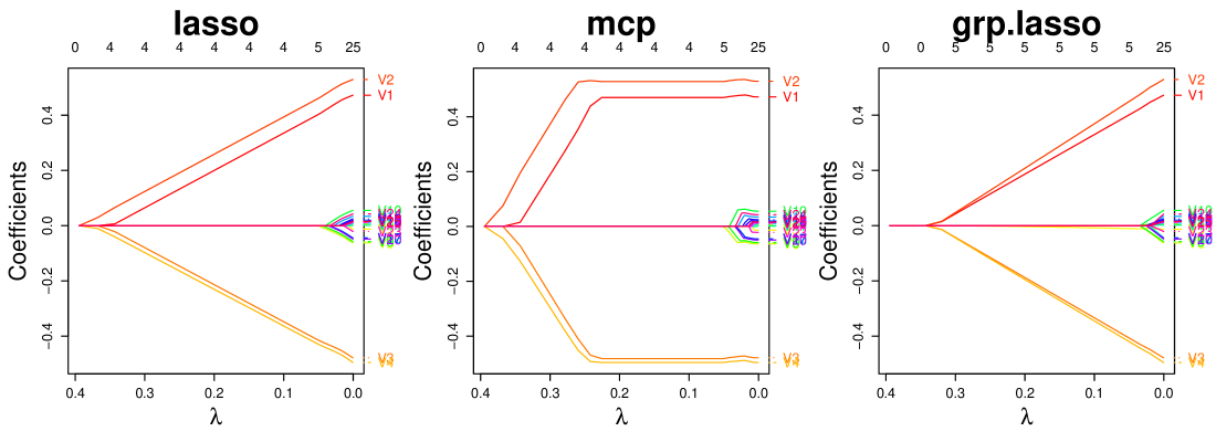
Figure 1: The plots above depict estimated coefficient paths for the lasso, MCP, and group lasso.

To compute the loss function in addition to the estimated coefficients, the argument compute.loss must be set to TRUE like the following:

fit <- oem(x = x, y = y, penalty = c("lasso", "mcp", "grp.lasso"), gamma = 2, groups = rep(1:5, each = 5), lambda.min.ratio = 1e-3, compute.loss = TRUE)

By default, compute.loss is set to FALSE because it adds a large computational burden, especially when many penalties are input. The function logLik.oemfit() can be used in complement with fitted with oem() objects with compute.loss = TRUE with the model specified using the which.model argument like the following:

logLik(fit, which.model = 2)[c(1, 25, 50, 100)] [1] -14189.39 -13804.72 -13795.76 -13795.11

5.2 Fitting multiple penalties

The OEM algorithm is well-suited to quickly estimate a solution path for multiple penalties simultaneously for the linear model if the number of variables is not too large, often when the number of variables is several thousand or fewer, provided the number of observations is larger than the number of variables. Ideally the number of observations should be at least ten times larger than the number of variables for best performance. Once the quantities $\bf A$ and $\mathbf{X}^{\top}\mathbf{y}$ are computed initially, then the remaining computational complexity for OEM for a given model and tuning parameter is just $O(p^{2})$ per iteration. To demonstrate the efficiency, consider the following simulated example:

nobs <- 1e6 nvars <- 100 rho <- 0.25 sigma <- matrix(rho, ncol = nvars, nrow = nvars) diag(sigma) <- 1 x2 <- mvrnorm(n = nobs, mu = numeric(nvars), Sigma = sigma) y2 <- drop(x2 rnorm(nobs, sd = 5)

mb <- microbenchmark( "oem[lasso]" = oem(x = x2, y = y2, penalty = c("lasso"), gamma = 3, groups = rep(1:20, each = 5)), "oem[all]" = oem(x = x2, y = y2, penalty = c("lasso", "mcp", "grp.lasso", "scad"), gamma = 3, groups = rep(1:20, each = 5)), times = 10L) print(mb, digits = 3) Unit: seconds expr min lq mean median uq max neval cld oem[lasso] 2.38 2.39 2.41 2.42 2.44 2.46 10 a oem[all] 2.88 2.89 2.92 2.91 2.93 3.00 10 b

5.3 Parallel support via OpenMP

As noted in Section 3, the key quantities necessary for the OEM algorithm can be computed in parallel. By specifying ncores to be a value greater than 1, the oem() function automatically employs OpenMP (OpenMP Architecture Review Board, 2015) to compute $\bf A$ and $\mathbf{X}^{\top}\mathbf{y}$ in parallel. Due to memory access inefficiencies in breaking up the computation of $\bf A$ into pieces, using multiple cores does not speed up computation linearly. It is typical for OpenMP not to result in linear speedups, especially on Windows machines, due to its overhead costs. Furthermore, if a user does not have OpenMP on their machine, the oem package will still run normally on one core. In the following example, we can see a slight benefit from invoking the use of extra cores.

nobs <- 1e5 nvars <- 500 rho <- 0.25 sigma <- rho ** abs(outer(1:nvars, 1:nvars, FUN = "-")) x2 <- mvrnorm(n = nobs, mu = numeric(nvars), Sigma = sigma) y2 <- drop(x2 rnorm(nobs, sd = 5) mb <- microbenchmark( "oem" = oem(x = x2, y = y2, penalty = c("lasso", "mcp", "grp.lasso", "scad"), gamma = 3, groups = rep(1:20, each = 25)), "oem[parallel]" = oem(x = x2, y = y2, ncores = 2, penalty = c("lasso", "mcp", "grp.lasso", "scad"), gamma = 3, groups = rep(1:20, each = 25)), times = 10L) print(mb, digits = 3) Unit: seconds expr min lq mean median uq max neval cld oem 4.80 4.85 4.93 4.93 5.00 5.07 10 b oem[parallel] 3.72 3.84 3.98 3.95 4.11 4.31 10 a

5.4 The cv.oem() function

The cv.oem() function is used for cross validation of penalized models fitted by the oem() function. It does not use the method described in Section 3 and hence can be used for models beyond the linear model. It can also benefit from parallelization using either OpenMP or the foreach package. For the former, one only need specify the ncores argument of cv.oem() and computation of the key quantities for OEM are computed in parallel for each cross validation fold. With the foreach package (Calaway et al., 2015b), cores must be “registered” in advance using doParallel (Calaway et al., 2015c), doMC (Calaway et al., 2015a), or otherwise. Each cross validation fold is computed on a separate core, which may be more efficient depending on the user’s hardware.

cvfit <- cv.oem(x = x, y = y, penalty = c("lasso", "mcp", "grp.lasso"), gamma = 2, groups = rep(1:5, each = 5), nfolds = 10)

The best performing model and its corresponding best tuning parameter can be accessed via:

cvfit$best.model\CodeOutput[1]"mcp"\CodeInput cvfit$lambda.min\CodeOutput[1]0.0739055\par Asummarymethodisavailableas\code{summary.cv.oem()},similartothesummaryfunctionof\code{cv.ncvreg()}ofthe\pkg{ncvreg}package,whichprintsoutputfromallofthecrossvalidatedmodels.Itcanbeusedlikethefollowing:\par\CodeChunk\CodeInput summary(cvfit)\CodeOutput lasso-penalizedlinearregressionwithn=10000,p=25Atminimumcross-validationerror(lambda=0.0242):-------------------------------------------------Nonzerocoefficients:13Cross-validationerror(Mean-SquaredError):9.11Scaleestimate(sigma):3.018\par<===============================================>\par mcp-penalizedlinearregressionwithn=10000,p=25Atminimumcross-validationerror(lambda=0.0739):-------------------------------------------------Nonzerocoefficients:5Cross-validationerror(Mean-SquaredError):9.10Scaleestimate(sigma):3.016\par<===============================================>\par grp.lasso-penalizedlinearregressionwithn=10000,p=25Atminimumcross-validationerror(lambda=0.0242):-------------------------------------------------Nonzerocoefficients:16Cross-validationerror(Mean-SquaredError):9.10Scaleestimate(sigma):3.017\par Predictionsfromanymodel(\code{which.model=2})orthebestofallmodels(\code{which.model="best.model"})using\code{cv.oem}objects.Thetuningparameterisspecifiedviatheargument\code{s},whichcantakenumericvaluesor\code{"lambda.min"}forthebesttuningparameteror\code{"lambda.1se"}foragoodbutmoreconservativetuningparameter.\par\CodeChunk\CodeInput predict(cvfit,newx=x[1:3,],which.model="best.model",s="lambda.min")\CodeOutput[,1][1,]-0.2233264[2,]0.2211386[3,]0.4760399\par$

5.5 The xval.oem() function

The xval.oem() function is much like cv.oem() but is limited to use for linear models only. It is significantly faster than cv.oem(), as it uses the method described in Section 3. Whereas cv.oem() functions by repeated calls to oem(), all of the primary computation in xval.oem() is carried out in C++. We chose to keep the xval.oem() function separate from the cv.oem() because the underlying code between the two methods is vastly different and furthermore because xval.oem() is not available for logistic regression models.

xvalfit <- xval.oem(x = x, y = y, penalty = c("lasso", "mcp", "grp.lasso"), gamma = 2, groups = rep(1:5, each = 5), nfolds = 10)

yrng <- range(c(unlist(xvalfit$cvup),unlist(xvalfit$cvlo))) layout(matrix(1:3, ncol = 3)) par(mar=c(5, 5, 5, 3) + 0.1) plot(xvalfit, which.model = 1, ylim = yrng, cex.main = 3, cex.axis = 1.25, cex.lab = 2) plot(xvalfit, which.model = 2, ylim = yrng, cex.main = 3, cex.axis = 1.25, cex.lab = 2) plot(xvalfit, which.model = 3, ylim = yrng, cex.main = 3, cex.axis = 1.25, cex.lab = 2)

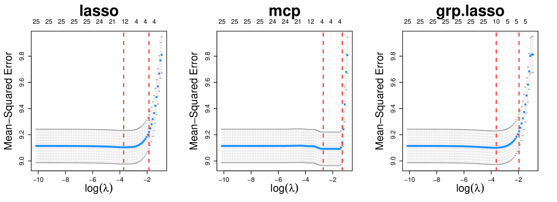
Figure 2: Depicted above are the cross validated mean squared prediction errors for paths of tuning parameters for the lasso, MCP, and group lasso.

5.6 OEM with precomputation for linear models with the oem.xtx() function

The key quantities, $\mathbf{X}^{\top}\mathbf{X}$ and $\mathbf{X}^{\top}\mathbf{y}$ can be computed in parallel, and when data are stored across a large cluster, their computation can be performed in a straightforward manner. When they are available, the oem.xtx() function can be used to carry out the OEM algorithm based on these quantities instead of on the full design matrix $\mathbf{X}$ and the full response vector $\mathbf{y}$. All methods available to objects fitted by oem() are also available to objects fitted by oem.xtx().

xtx <- crossprod(x) / nrow(x) xty <- crossprod(x, y) / nrow(x)

fitxtx <- oem.xtx(xtx, xty, penalty = c("lasso", "mcp", "grp.lasso"), gamma = 2, groups = rep(1:5, each = 5))

5.7 Out-of-Memory computation with the big.oem() function

Standard R objects are stored in memory and thus, when a design matrix is too large for memory it cannot be used for computation in the standard way. The bigmemory package offers objects which point to data stored on disk and thus allows users to bypass memory limitations. It also provides access to C++ objects which do the same. These objects are highly efficient due to memory mapping, which is a method of mapping a data file to virtual memory and allows for efficient moving of data in and out of memory from disk. For further details on memory mapping, we refer readers to Bovet and Cesati (2005); Kane et al. (2013). The big.oem() function allows for out-of-memory computation by linking Eigen matrix objects to data stored on disk via bigmemory.

The standard approach for loading the data from SEXP objects (X_ in the example below) to Eigen matrix objects (X in the example below) in C++ looks like:

using Eigen::Map; using Eigen::MatrixXd; const Map<MatrixXd> X(as<Map<MatrixXd> >(X_));

To instead map from an object which is a pointer to data on disk, we first need to load the bigmemory headers:

#include <bigmemory/MatrixAccessor.hpp> #include <bigmemory/BigMatrix.h>

Then we link the pointer (passed from R to C++ as X_ and set as bigPtr below) to data to an Eigen matrix object via:

XPtr<BigMatrix> bigPtr(X_); const Map<MatrixXd> X = Map<MatrixXd> ((double *)bigPtr->matrix(), bigPtr->nrow(), bigPtr->ncol() );

The remaining computation for OEM is carried out similarly as for oem(), yet here the object X is not stored in memory.

To test out big.oem() and demonstrate its memory usage profile we simulate a large dataset and save it as a “filebacked” big.matrix object from the bigmemory package.

nobs <- 1e6 nvars <- 250 bkFile <- "big_matrix.bk" descFile <- "big_matrix.desc" big_mat <- filebacked.big.matrix(nrow = nobs, ncol = nvars, type = "double", backingfile = bkFile, backingpath = ".", descriptorfile = descFile, dimnames = c(NULL, NULL))

for (i in 1:nvars) big_mat[, i] = rnorm(nobs)

yb <- rnorm(nobs, sd = 5)

Using the profvis() function of the profvis package (Chang et al., 2016), we can see that no copies of the design matrix are made at any point. Furthermore, a maximum of 173 Megabytes are used by the R session during this simulation, whereas the size of the design matrix is 1.9 Gigabytes. The following code generates an interactive html visualization of the memory usage of big.oem() line-by-line:

profvis::profvis( bigfit <- big.oem(x = big_mat, y = yb, penalty = c("lasso", "grp.lasso", "mcp", "scad"), gamma = 3, groups = rep(1:50, each = 5)) )

Here we save a copy of the design matrix in memory for use by oem():

xb <- big_mat[,]

print(object.size(xb), units = "Mb") 1907.3 Mb print(object.size(big_mat), units = "Mb") 0 Mb

The following benchmark for on-disk computation is on a system with a hard drive with 7200 RPM, 16MB Cache, and SATA 3.0 Gigabytes per second (a quite modest setup compared with a system with a solid state drive). Even without a solid state drive we pay little time penalty for computing on disk over computing in memory.

mb <- microbenchmark( "big.oem" = big.oem(x = big_mat, y = yb, penalty = c("lasso", "grp.lasso", "mcp", "scad"), gamma = 3, groups = rep(1:50, each = 5)), "oem" = oem(x = xb, y = yb, penalty = c("lasso", "grp.lasso", "mcp", "scad"), gamma = 3, groups = rep(1:50, each = 5)), times = 10L)

print(mb, digits = 3) Unit: seconds expr min lq mean median uq max neval cld big.oem 8.46 8.51 8.73 8.57 8.69 9.73 10 a oem 9.81 9.85 10.36 10.08 10.65 12.03 10 b

5.8 Sparse matrix support

The oem() and cv.oem() functions can accept sparse design matrices as provided by the CsparseMatrix class of objects of the Matrix package (Bates and Maechler, 2016). If the design matrix provided has a high degree of sparsity, using a CsparseMatrix object can result in a substantial computational speedup and reduction in memory usage.

library(Matrix) n.obs <- 1e5 n.vars <- 200 true.beta <- c(runif(15, -0.25, 0.25), rep(0, n.vars - 15)) xs <- rsparsematrix(n.obs, n.vars, density = 0.01) ys <- rnorm(n.obs, sd = 3) + as.vector(xs x.dense <- as.matrix(xs)

mb <- microbenchmark(fit = oem(x = x.dense, y = ys, penalty = c("lasso", "grp.lasso"), groups = rep(1:40, each = 5)), fit.s = oem(x = xs, y = ys, penalty = c("lasso", "grp.lasso"), groups = rep(1:40, each = 5)), times = 10L)

print(mb, digits = 3) Unit: milliseconds expr min lq mean median uq max neval cld fit 669.9 672.5 679.3 680.3 682.2 690.6 10 b fit.s 63.2 64.1 65.5 65.3 66.8 68.2 10 a

5.9 API comparison with glmnet

The application program interface (API) of the oem package was designed to be familiar to users of the glmnet package. Data ready for use by glmnet() can be used directly by oem(). Most of the arguments are the same, except the penalty argument and other arguments relevant to the various penalties available in oem().

Here we fit linear models with a lasso penalty using oem() and glmnet():

oem.fit <- oem(x = x, y = y, penalty = "lasso") glmnet.fit <- glmnet(x = x, y = y)

Here we fit linear models with a lasso penalty using oem() and glmnet() with sparse design matrices:

oem.fit.sp <- oem(x = xs, y = ys, penalty = "lasso") glmnet.fit.sp <- glmnet(x = xs, y = ys)

Now we make predictions using the fitted model objects from both packages:

preds.oem <- predict(oem.fit, newx = x) preds.glmnet <- predict(glmnet.fit, newx = x)

We now plot the coefficient paths using both fitted model objects:

plot(oem.fit, xvar = "norm") plot(glmnet.fit, xvar = "norm")

We now fit linear models with a lasso penalty and select the tuning parameter with cross validation using cv.oem(), xval.oem(), and cv.glmnet():

oem.cv.fit <- cv.oem(x = x, y = y, penalty = "lasso") oem.xv.fit <- xval.oem(x = x, y = y, penalty = "lasso") glmnet.cv.fit <- cv.glmnet(x = x, y = y)

We now plot the cross validation errors using all fitted cross validation model objects:

plot(oem.cv.fit) plot(oem.xv.fit) plot(glmnet.cv.fit)

We now make predictions using the best tuning parameter according to cross validation error using all fitted cross validation model objects:

preds.cv.oem <- predict(oem.cv.fit, newx = x, s = "lambda.min") preds.xv.oem <- predict(oem.xv.fit, newx = x, s = "lambda.min") preds.cv.glmnet <- predict(glmnet.cv.fit, newx = x, s = "lambda.min")

6 Timings

Extensive numerical studies are conducted in Xiong et al. (2016) regarding the OEM algorithm for computation time for paths of tuning parameters for various penalties, so in the following simulation studies, we will focus on computation time for the special features of the oem package such as cross validation and sparse matrix support. All simulations are run on a 64-bit machine with an Intel Xeon E5-2470 2.30 GHz CPU and 128 Gigabytes of main memory and a Linux operating system.

6.1 Cross validation

In this section we will compare the computation time of the cv.oem() and xval.oem() for various penalties, both individually and simultanously, with the cross validation functions from other various packages, including glmnet, ncvreg, grpreg, gglasso, and the Python package sklearn (Pedregosa et al., 2011). The model class we use from sklearn is LassoCV, which performs cross validation for lasso linear models. In particular, we focus on the comparison with glmnet, as it has been carefully developed with computation time in mind and has long been the gold standard for computational performance.

In the simulation setup, we generate the design matrix from a multivariate normal distribution with covariance matrix $(\sigma_{ij})=0.5^{|i-j|}$. Responses are generated from the following model:

$$\mathbf{y}=\mathbf{X}\bm{\beta}+\bm{\epsilon}$$

where the first five elements of $\bm{\beta}$ are $(-0.5,-0.5,0.5,0.5,1)$ and the remaining are zero and $\bm{\epsilon}$ is an independent mean zero normal random variable with standard deviation 2. The total number of observations $n$ is set to $10^{5}$ and $10^{6}$, the number of variables $p$ is varied from 50 to 500, and the number of folds for cross validation is set to 10. For grouped regularization, groups of variables of size 25 are chosen contiguously. For the MCP regularization, the tuning parameter $\gamma$ is chosen to be 3. Each method is fit using the same sequence of 100 values of the tuning parameter $\lambda$ and convergence is specified to be the same level of precision for each method. The computation times for the glmnet and oem functions without cross validation are given as a reference point.

From the results in Figure 3, both the xval.oem() and cv.oem() functions are competitive with all other cross validation alternatives. Surprisingly, the xval.oem() function for the lasso penalty only is competitive with and in many scenarios is even faster than glmnet, which does not perform cross validation. The xval.oem() is clearly faster than cv.oem() in all scenarios. In many scenarios cv.oem() takes at least 6 times longer than xval.oem(). Both cross validation functions from the oem package are nearly as fast in computing for three penalties simultaneously as they are for just one. We have found in general that for any scenario where $n>>p$ and cross validation is required, it is worth considering oem as a fast alternative to other packages. In particular, a rough rule of thumb is that oem is advantageous when $n>10p$, however, oem may be advantageous with fewer observations than this for penalties other than the lasso, such as MCP, SCAD, and group lasso.

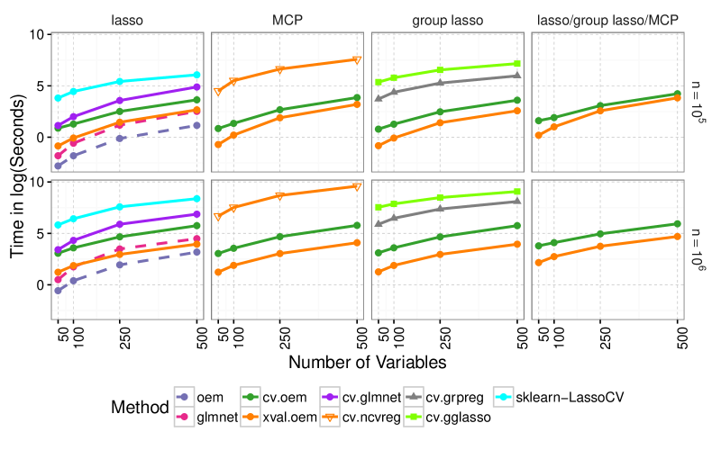
Figure 3: Depicted above is the average computing time over ten runs in log(Seconds) for the functions that perform cross validation for selection of the tuning parameter for various penalized regression methods.

Now we test the impact of parallelization on the computation time of xval.oem() using the same simulation setup as above except now we additionally vary the number of cores used. From the results in Figure 4, we can see that using parallelization through OpenMP helps to some degree. However, it is important to note that using more cores than the number of cross validation folds will unlikely result in better computation time than the same number of cores as the number of folds due to how parallelization is implemented.

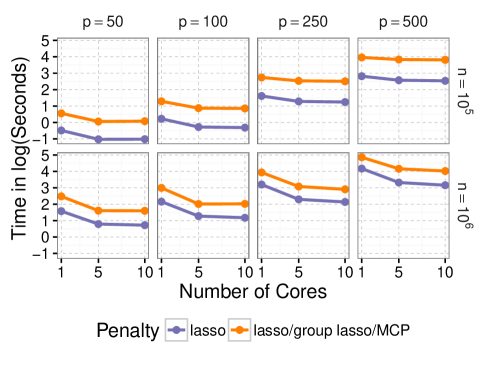
Figure 4: Depicted above is the average computing time over ten runs in log(Seconds) for the xval.oem() function with a varying number of cores. Results are shown for just one penalty (lasso) and three penalties fit simultaneously (lasso, group lasso, and MCP) with 100 values for the tuning parameter $\lambda$ for each penalty.

6.2 Sparse matrices

In the following simulated example, sparse design matrices are generated using the function rsparsematrix() of the Matrix package with nonzero entries generated from an independent standard normal distribution. The proportion of zero entries in the design matrix is set to 0.99, 0.95, and 0.9. The total number of observations $n$ is set to $10^{5}$ and $10^{6}$ and the number of variables $p$ is varied from 250 to 1000. Responses are generated from the same model as in Section 6.1. Each method is fit using the same sequence of 100 values of the tuning parameter $\lambda$ and convergence is specified to be the same level of precision for each method. The authors are not aware of penalized regression packages other than glmnet that provide support for sparse matrices, so we just compare oem with glmnet. From the results in Figure 5, it can be seen that oem() is superior in computation time for very tall data settings with a high degree of sparsity of the design matrix.

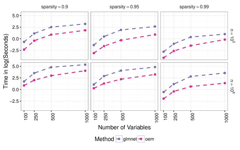
Figure 5: Depicted above is the average computing time over ten runs in log(Seconds) for computation of lasso linear regression models using sparse matrices.

6.3 Penalized logistic regression

In this simulation, we generate the design matrix from a multivariate normal distribution with covariance matrix $(\sigma_{ij})=0.5^{|i-j|}$. Responses are generated from the following model:

$$\mbox{Pr}(Y_{i}=\bm{1}|x_{i})=\frac{1}{1+\exp{(-x_{i}^{\top}\bm{\beta})}},\mbox{ for }i=1,\dots,n$$

where the first five elements of $\bm{\beta}$ are $(-0.5,-0.5,0.5,0.5,1)$ and the remaining are zero. The total number of observations $n$ is set to $10^{4}$ and $10^{5}$, the number of variables $p$ is varied from 50 to 500. For grouped regularization, groups of variables of size 25 are chosen contiguously. For the MCP regularization, the tuning parameter $\gamma$ is chosen to be 3. Each method is fit using the same sequence of 25 values of the tuning parameter $\lambda$. Both glmnet() and oem() allow for a Hessian upper-bound approximation for logistic regression models, so in this simulation we compare both the vanilla versions of each in addition to the Hessian upper-bound versions. For logistic regression models, unlike linear regression, the various functions compared use vastly different convergence criterion, so care was taken to set the convergence thresholds for the different methods to achieve a similar level of precision.

The average computing times over 10 runs are displayed in Figure 6. The Hessian upper-bound versions of glmnet() and oem() are given by the dashed lines. The glmnet() function is the fastest for lasso-penalized logistic regression, but oem() with an without the use of a Hessian upper-bound is nearly as fast as glmnet() when the sample size gets larger. For the MCP and group lasso, oem() with the Hessian upper-bound option is the fastest across the vast majority of simulation settings. In general, the Hessian upper-bound is most advantageous when the number of variables is moderately large.

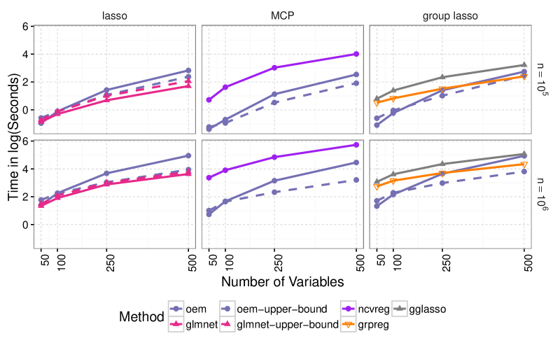
Figure 6: Depicted above is the average computing time over ten runs in log(Seconds) for the functions that penalized estimates for binomial regression models.

6.4 Quality of solutions

In this section we present information about the quality of solutions provided by each of the compared packages. Using the same simulation setup and precisions for convergence as the cross validation and binomial simulations, we investigate the numerical precision of the methods by presenting the objective function values corresponding to the given solutions. Specifically, we look at the difference in the objective function values between oem() and the comparative functions. A Negative value here indicates that the oem() function results in solutions with a smaller value of the objective function. Since each simulation is run on a sequence of tuning parameter values we present the differences in objective functions averaged over the tuning parameters. Since the objective function values across the different tuning parameter values are on the same scale, this comparison is reasonable. While the grpreg() function from the grpreg package provides solutions for the group lasso, it minimizes a slightly modified objective function, wherein the covariates are orthonormalized within groups as described in Section 2.1 of Breheny and Huang (2015). Due to this fact we do not compare the objective function values assocated with results returned by grpreg().

The objective function value differences for the linear model simulations are presented in Table 2. We can see that the solutions provided by oem() are generally more precise than those of other functions except ncvreg() for the MCP. However, the differences between the solutions provided by oem() and ncvreg() for the MCP are close to machine precision. The objective function value differences for the logistic model simulations are presented in Tables 3 and 4. Table 3 refers to comparisons between oem() using the full Hessian and other methods and Table 4 refers to comparisons between oem() using the Hessian upper-bound. We can see that oem() in both cases results in solutions which are generally more precise than other methods. Interestingly, for the logistic regression simulations unlike the linear regression simulations, we see that oem() provides solutions which are dramatically more precise than ncvreg() for the MCP. These results indicate that the nonconvexity of the MCP has more serious consequences for logistic regression in terms of algorithmic choices.

$n$	$p$	glmnet	gglasso	ncvreg
$10^{5}$	50	$-4.50^{-09}$	$-3.46^{-06}$	$\hphantom{-}2.47^{-11}$
	100	$-5.38^{-09}$	$-3.38^{-06}$	$-1.46^{-12}$
	250	$-1.93^{-08}$	$-3.37^{-06}$	$-1.15^{-12}$
	500	$-3.58^{-08}$	$-3.29^{-06}$	$\hphantom{-}7.11^{-12}$
$10^{6}$	50	$-2.00^{-09}$	$-3.32^{-06}$	$\hphantom{-}7.00^{-14}$
	100	$-4.34^{-09}$	$-3.30^{-06}$	$-1.39^{-14}$
	250	$-8.82^{-09}$	$-3.36^{-06}$	$\hphantom{-}6.76^{-12}$
	500	$-1.75^{-08}$	$-3.34^{-06}$	$\hphantom{-}1.69^{-14}$

Table 2: The results above are the averages differences between the oem() function and other methods in objective function values averaged over all of the values of the tuning parameter for the linear regression simulations. Negative here means the oem() function results in estimates with a lower objective function value.

$n$	$p$	glmnet	glmnet (ub)	gglasso	ncvreg
$10^{4}$	50	$-2.79^{-13}$	$-4.30^{-12}$	$-4.33^{-07}$	$-5.31^{-03}$
	100	$-1.82^{-13}$	$-4.74^{-12}$	$-4.95^{-07}$	$-4.90^{-03}$
	250	$-6.52^{-13}$	$-3.87^{-12}$	$-5.06^{-07}$	$-5.03^{-03}$
	500	$-4.80^{-13}$	$-6.90^{-12}$	$-5.30^{-07}$	$-5.48^{-03}$
$10^{5}$	50	$-1.48^{-13}$	$-2.72^{-12}$	$-4.79^{-07}$	$-3.05^{-03}$
	100	$-1.30^{-13}$	$-2.17^{-12}$	$-4.78^{-07}$	$-4.55^{-03}$
	250	$-9.30^{-14}$	$-2.78^{-12}$	$-4.78^{-07}$	$-4.47^{-03}$
	500	$-2.07^{-13}$	$-4.49^{-12}$	$-4.51^{-07}$	$-3.07^{-03}$

Table 3: The results above are the averages differences between the full Hessian version of oem() and other methods in objective function values averaged over all of the values of the tuning parameter for the logistic regression simulations. Negative here means the oem() function results in estimates with a lower objective function value. The heading “glmnet (ub)” corresponds to glmnet() with the Hessian upper bound option.

$n$	$p$	glmnet	glmnet (ub)	gglasso	ncvreg
$10^{4}$	50	$-7.01^{-14}$	$-4.09^{-12}$	$-4.20^{-07}$	$-5.31^{-03}$
	100	$\hphantom{-}6.74^{-13}$	$-3.88^{-12}$	$-4.76^{-07}$	$-4.90^{-03}$
	250	$-3.88^{-14}$	$-3.25^{-12}$	$-4.97^{-07}$	$-5.03^{-03}$
	500	$-4.06^{-13}$	$-6.82^{-12}$	$-5.16^{-07}$	$-5.47^{-03}$
$10^{5}$	50	$\hphantom{-}3.16^{-12}$	$\hphantom{-}5.87^{-13}$	$-4.71^{-07}$	$-3.05^{-03}$
	100	$\hphantom{-}3.06^{-12}$	$\hphantom{-}1.02^{-12}$	$-4.61^{-07}$	$-4.55^{-03}$
	250	$\hphantom{-}2.72^{-12}$	$\hphantom{-}3.40^{-14}$	$-4.71^{-07}$	$-4.47^{-03}$
	500	$\hphantom{-}1.09^{-12}$	$-3.19^{-12}$	$-4.31^{-07}$	$-3.07^{-03}$

Table 4: The results above are the averages differences between the upper bound version of oem() and other methods in objective function values averaged over all of the values of the tuning parameter for the logistic regression simulations. Negative here means the oem() function results in estimates with a lower objective function value. The heading “glmnet (ub)” corresponds to glmnet() with the Hessian upper bound option.

7 Acknowledgments

This material is based upon work supported by, or in part by, the U. S. Army Research Laboratory and the U. S. Army Research Office under contract/grant number W911NF1510156, NSF Grants DMS 1055214 and DMS 1564376, and NIH grant T32HL083806.

References

- Bates et al. (2016) Bates D, Eddelbuettel D, Francois R, Qiu Y, the authors of \pkgEigen for the included version of \pkgEigen (2016). \pkgRcppEigen: ‘\pkgRcpp’ Integration for the ‘\pkgEigen’ Templated Linear Algebra Library. \proglangR package version 0.3.2.9.0, URL https://CRAN.R-project.org/package=RcppEigen.
- Bates and Maechler (2016) Bates D, Maechler M (2016). \pkgMatrix: Sparse and Dense Matrix Classes and Methods. \proglangR package version 1.2-7.1, URL https://CRAN.R-project.org/package=Matrix.
- Bovet and Cesati (2005) Bovet D, Cesati M (2005). Understanding the Linux Kernel. O’Reilly Media, Inc.
- Breheny (2016) Breheny P (2016). \pkggrpreg: Regularization Paths for Regression Models with Grouped Covariates. \proglangR package version 3.0-2, URL https://CRAN.R-project.org/package=grpreg.
- Breheny and Huang (2015) Breheny P, Huang J (2015). “Group descent algorithms for nonconvex penalized linear and logistic regression models with grouped predictors.” Statistics and Computing, 25(2), 173–187.
- Breheny and Lee (2016) Breheny P, Lee S (2016). \pkgncvreg: Regularization Paths for SCAD and MCP Penalized Regression Models. \proglangR package version 3.6-0, URL https://CRAN.R-project.org/package=ncvreg.
- Calaway et al. (2015a) Calaway R, Revolution Analytics, Weston S (2015a). \pkgdoMC: \pkgForeach Parallel Adaptor for ‘\pkgparallel’. \proglangR package version 1.3.4, URL https://CRAN.R-project.org/package=doMC.
- Calaway et al. (2015b) Calaway R, Revolution Analytics, Weston S (2015b). \pkgforeach: Sparse and Dense Matrix Classes and Methods. \proglangR package version 1.4.3, URL https://CRAN.R-project.org/package=foreach.
- Calaway et al. (2015c) Calaway R, Revolution Analytics, Weston S, Tenenbaum D (2015c). \pkgdoParallel: \pkgForeach Parallel Adaptor for the ‘\pkgparallel’ Package. \proglangR package version 1.0.10, URL https://CRAN.R-project.org/package=doParallel.
- Chang et al. (2016) Chang W, Luraschi J, RStudio, jQuery Foundation, jQuery contributors, Mike Bostock, D3 contributors, Ivan Sagalaev (2016). \pkgprofvis: Interactive Visualizations for Profiling R Code. \proglangR package version 0.3.2, URL https://CRAN.R-project.org/package=profvis.
- Efron et al. (2004) Efron B, Hastie T, Johnstone I, Tibshirani R (2004). “Least Angle Regression.” The Annals of Statistics, 32(2), 407–499.
- Fan and Li (2001) Fan J, Li R (2001). “Variable Selection via Nonconcave Penalized Likelihood and Its Oracle Properties.” Journal of the American Statistical Association, 96(456), 1348–1360.
- Friedman et al. (2016) Friedman J, Hastie T, Simon N, Tibshirani R (2016). \pkgglmnet: Lasso and Elastic-Net Regularized Generalized Linear Models. \proglangR package version 2.0-5, URL https://CRAN.R-project.org/package=glmnet.
- Friedman et al. (2010) Friedman JH, Hastie T, Tibshirani R (2010). “Regularization Paths for Generalized Linear Models via Coordinate Descent.” Journal of Statistical Software, 33(1), 1–22. ISSN 1548-7660.
- Guennebaud et al. (2010) Guennebaud G, Jacob B, et al. (2010). “\pkgEigen v3.” http://eigen.tuxfamily.org.
- Hastie and Efron (2013) Hastie T, Efron B (2013). \pkglars: Least Angle Regression, Lasso and Forward Stagewise. \proglangR package version 1.2, URL https://CRAN.R-project.org/package=lars.
- Healy and Westmacott (1956) Healy, Westmacott (1956). “Missing Values in Experiments Analysed on Automatic Computers.” Applied Statistics, 5, 203–206. ISSN 0885-7474.
- Jenatton et al. (2010) Jenatton R, Mairal J, Bach FR, Obozinski GR (2010). “Proximal methods for sparse hierarchical dictionary learning.” In Proceedings of the 27th international conference on machine learning, pp. 487–494.
- Kane et al. (2016) Kane MJ, Emerson JW, Haverty P, Jr CD (2016). \pkgbigmemory: Manage Massive Matrices with Shared Memory and Memory-Mapped Files. \proglangR package version 4.5.19, URL https://CRAN.R-project.org/package=bigmemory.
- Kane et al. (2013) Kane MJ, Emerson JW, Weston S (2013). “Scalable Strategies for Computing with Massive Data.” Journal of Statistical Software, 55(1), 1–19. 10.18637/jss.v055.i14. URL https://www.jstatsoft.org/index.php/jss/article/view/v055i14.
- Krishnapuram et al. (2005) Krishnapuram B, Carin L, Figueiredo MA, Hartemink AJ (2005). “Sparse multinomial logistic regression: Fast algorithms and generalization bounds.” IEEE transactions on Pattern Analysis and Machine Intelligence, 27(6), 957–968.
- Lanczos (1950) Lanczos C (1950). “An Iteration Method for the Solution of the Eigenvalue Problem of Linear Differential and Integral Operators.” Journal of Research of the National Bureau of Standards, 45, 255–282.
- \pkgOpenMP Architecture Review Board (2015) \pkgOpenMP Architecture Review Board (2015). \pkgOpenMP Application Program Interface Version 4.5. URL http://www.openmp.org/wp-content/uploads/openmp-4.5.pdf.
- Pedregosa et al. (2011) Pedregosa F, Varoquaux G, Gramfort A, Michel V, Thirion B, Grisel O, Blondel M, Prettenhofer P, Weiss R, Dubourg V, Vanderplas J, Passos A, Cournapeau D, Brucher M, Perrot M, Édouard Duchesnay (2011). “Scikit-learn: Machine Learning in Python.” Journal of Machine Learning Research, 12, 2825–2830. \proglangPython package version 0.18.1, URL http://dl.acm.org/citation.cfm?id=1953048.2078195.
- Tibshirani (1996) Tibshirani R (1996). “Regression Shrinkage and Selection via the Lasso.” Journal of the Royal Statistical Society B, pp. 267–288.
- Tseng (2001) Tseng P (2001). “Convergence of a Block Coordinate Descent Method for Nondifferentiable Minimization.” Journal of Optimization Theory and Applications, 109(3), 475–494.
- Xiong et al. (2016) Xiong S, Dai B, Huling J, Qian PZG (2016). “Orthogonalizing EM: A Design-Based Least Squares Algorithm.” Technometrics, 58(3), 285–293.
- Yang and Zou (2014) Yang Y, Zou H (2014). \pkggglasso: Group Lasso Penalized Learning Using a Unified BMD Algorithm. \proglangR package version 1.3, URL https://CRAN.R-project.org/package=gglasso.
- Yuan and Lin (2006) Yuan M, Lin Y (2006). “Model Selection and Estimation in Regression with Grouped Variables.” Journal of the Royal Statistical Society B, 68(1), 49–67.
- Zeng and Breheny (2016) Zeng Y, Breheny P (2016). \pkgbiglasso: Big Lasso: Extending Lasso Model Fitting to Big Data in \pkgR. \proglangR package version 1.2-3, URL https://CRAN.R-project.org/package=biglasso.
- Zhang (2010) Zhang CH (2010). “Nearly Unbiased Variable Selection Under Minimax Concave Penalty.” The Annals of Statistics, 38(2), 894–942.