Emergent Dark Energy from Dark Matter

Abstract

We consider the cosmological dynamics of a scalar field in a potential with multiple troughs and peaks. We show that the dynamics of the scalar field will evolve from light dark matter-like behaviour (such as that of a light axion) to a combination of heavy dark matter-like and dark energy-like behaviour. We discuss the phenomenology of such a model, explaining how it can give rise to the cosmological constant, as well as how it can decouple the dark sector densities between the time of recombination and today, for both the homogeneous background and perturbations. The final form of the dark matter is axion-like, but with abundance and primordial isocurvature modes taking very different values from traditional, axionic, dark matter.

Introduction: Scalar fields have played an important role in modern theoretical cosmology. They have been at the heart of inflationary cosmology, driving the accelerated expansion at early times Martin:2013tda . They have been invoked as a plausible candidate for dark matter, in the form of an axion or axion-like particles Arvanitaki:2009fg ; Ringwald:2012hr ; Marsh:2015xka ; Hui:2016ltb . And they are the leading candidate for dark energy, replacing the cosmological constant as the dominant energy source at late times Copeland:2006wr ; Clifton:2011jh .

The standard approach has been to consider models which have some fundamental underpinning. Typically this involves choosing a potential $V(\phi)$ for the scalar field, $\phi$, with a simple analytic form, with one or a few minima, or with a certain degree of periodicity. The resulting dynamics is often relatively simple: the dynamics of the scalar field is either monotonic (used for inflation and dark energy) or oscillatory (used for dark matter). It would make sense, however, to countenance the possibility that $V(\phi)$ is rich, structured, with many different scales and minima. Such a complex potential can easily arise if one considers multiple scalar fields, or in higher-dimensional universe, with many extra dimensions and highly intricate topologies Sloan:2016kbc . A particularly interesting analogy that can be considered is with spin-glasses where multiple minima can lead to rich dynamics and complex phenomena Soljacic:1999im . In this paper we will explore the possibility that, at late times, a cosmological scalar field is embedded in a theory which has a high degree of complexity and show that novel dynamics can emerge.

We will consider a scenario with one degree of freedom, i.e. one scalar field, that resides in an effective potential with structures on different scales. Its origin may be in a multi-dimensional field space, such as the string landscape or axiverse Douglas:2006es ; Arvanitaki:2009fg , but for the purpose of this paper, we will model it as $V(\phi)$. This can be viewed as focusing on the lightest direction in the multi-field space. It is also known that, under certain symmetries, a multi-scalar field theory can relax to lower dimensional dynamics (for an interesting example involving scale symmetry, see Ferreira:2016vsc ; Ferreira:2016wem ). An example of the type of potential we are envisaging can be seen in Figure 1 where successive “zoom ins” of the potential close to what looks like the global minimum reveals a rich structure of local minima. This “zoom in” naturally occurs for a cosmological scalar field oscillating along the potential, since the expansion of the universe forces the oscillation to damp. As a consequence, the oscillating scalar eventually gets trapped in one of the local minima of the substructure. We will show that this picture corresponds to a universe with dark matter occasionally splitting into a mixture of dark matter plus dark energy, and explore its phenomenological and cosmological consequences.

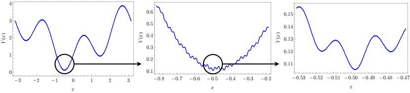
Figure 1: Cartoon of a scalar field potential with structure. As the universe expands and the scalar oscillation is damped, the scalar field ‘discovers’ more local minima of the potential.

Two-cosine model: Let us consider a minimally coupled real scalar field with an action

$$S=\int d^{4}x\sqrt{-g}\left[\frac{M^{2}_{\rm Pl}}{2}R-\frac{1}{2}g^{\mu\nu}\partial_{\mu}\phi\partial_{\nu}\phi-V(\phi)+L_{\mathrm{m}}\right],$$ (1)

where $L_{\mathrm{m}}$ is the Lagrangian for other matter fields. If we restrict ourselves to a homogeneous and isotropic space-time, with $ds^{2}=-dt^{2}+a^{2}(t)(d\vec{r})^{2}$, we arrive at the Klein-Gordon equation ${\ddot{\phi}}+3H{\dot{\phi}}=-V^{\prime}$ and the Friedmann equation $3M^{2}_{\rm Pl}H^{2}=\rho_{\phi}+\rho_{\mathrm{m}}$. Here overdot is derivative with regards to $t$, $H={\dot{a}}/a$, $V^{\prime}=dV/d\phi$, and $\rho_{\phi}=V+\dot{\phi}^{2}/2$ is the scalar field energy density. Two salient regimes should be highlighted. If $V\simeq m^{2}\phi^{2}/2$ and $m\gg H$, then $\phi$ will be oscillatory and $\rho_{\phi}\propto 1/a^{3}$; the scalar field will evolve as a cold dark matter component. If $V\simeq V_{0}$ and $V_{0}\gg{\dot{\phi}}^{2}$, then $\rho_{\phi}$ will play the role of a cosmological constant and, if further $\rho_{\mathrm{m}}\ll\rho_{\phi}$ we have $H\simeq$ constant.

As the simplest potential that exhibits structures on different scales, let us consider a potential consisting of two cosines:

$$V(\phi)=V_{0}+m^{2}f^{2}\left\{1-\cos\left(\frac{\phi}{f}\right)+c\left[1-\cos\left(n\frac{\phi}{f}+\delta\right)\right]\right\}.$$ (2)

Here $V_{0}$ is an offset with mass dimension four, $m$ and $f$ are mass scales, and $c$, $n$, and $\delta$ are dimensionless. We choose $m,f,c>0$ and $n>1$. The $\cos(\phi/f)$ sets the global structure while $\cos(n\phi/f+\delta)$ sets the substructure of the potential. One can easily check that when $cn^{2}\ll 1$, the extrema of the potential are mainly set by $\cos(\phi/f)$ and thus appear only around $\phi/f=0,\pm\pi,\pm 2\pi,\cdots$. In such a case the potential is effectively a single cosine. If, on the other hand, $cn\gg 1$, the positions of the extrema are determined by $\cos(n\phi/f+\delta)$. Once the scalar starts oscillating along this potential, it will quickly get trapped in one of the local minima of the substructure.

The case of interest for our purpose is

$$cn\ll 1\ll cn^{2},$$ (3)

which implies $c\ll 1$ and $n\gg 1$. In such a case the $\cos(n\phi/f+\delta)$ term in the potential produces extrema, but only within the distance of $\Delta\phi/f\sim cn$ from the extrema of $\cos(\phi/f)$. Let us focus on this case and consider the dynamics of a homogeneous scalar field along the two-cosine potential.

Assuming that the initial position of the scalar field $\phi_{*}$ is located in the region $cn<\lvert\phi_{*}\rvert/f\lesssim 1$, then its dynamics at the beginning is set by the $\cos(\phi/f)$ term in the potential, giving the scalar an effective mass of $m$. Hence the field is initially frozen at $\phi_{*}$ due to the Hubble friction while $H>m$, and then starts to oscillate when $H\sim m$ foot1 .

After the onset of the oscillation, it is useful to split the scalar density as $\rho_{\phi}=\rho_{\mathrm{vac}}+\rho_{\mathrm{osc}}$, where the first term denotes the vacuum energy $\rho_{\mathrm{vac}}=V(\phi_{\mathrm{gl}})$ at the global minimum $\phi_{\mathrm{gl}}$ of the potential, and the rest we refer to as the oscillation energy $\rho_{\mathrm{osc}}$. The potential is well approximated by a quadratic except for the tiny region within $|\phi|/f\lesssim cn$, hence the oscillation is approximately harmonic and damped by the expansion of the universe, so that $\rho_{\mathrm{osc}}\propto 1/a^{3}$.

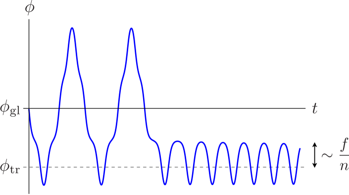
Figure 2: An example trajectory of a scalar field being trapped in a local minimum of the two-cosine potential (2).

When the oscillation amplitude $\bar{\phi}$ becomes sufficiently small, $\bar{\phi}/f\sim cn$, the finer structure of the potential becomes relevant and the scalar field eventually becomes trapped in one of the local minima created by the $\cos(n\phi/f+\delta)$. (It is also possible that the field gets trapped in the potential well around the global minimum, however we do not consider such a case.) The trapping minimum, which we represent by $\phi_{\mathrm{tr}}$, lies within the range of

$$\frac{2\pi}{n}\lesssim\frac{\lvert\phi_{\mathrm{tr}}\rvert}{f}\lesssim cn.$$ (4)

Here the lower bound comes from the fact that each minimum is separated from their adjacent ones by $\Delta\phi/f\sim 2\pi/n$, and the assumption of $\phi_{\mathrm{tr}}\neq\phi_{\mathrm{gl}}$. It is not an easy task to obtain a general prediction of the value of $\phi_{\mathrm{tr}}$ within the above range. One may expect the field to be trapped at a minimum near the upper end $\lvert\phi_{\mathrm{tr}}\rvert/f\sim cn$, however there the potential well is shallow and thus the trapping probability is not necessarily high. Furthermore, $\phi_{\mathrm{tr}}$ is determined not just by the initial condition $\phi_{*}$, but also by the Hubble rate during trapping. In the following discussions we treat $\phi_{\mathrm{tr}}$ as a free parameter within the range (4). An example of the scalar field trajectory upon trapping for a case with $\lvert\phi_{\mathrm{tr}}\rvert/f\sim 2\pi/n$ is shown in Figure 2, which we have obtained by numerically computing the equations of motion.

After the trapping, the scalar’s effective mass has increased to $m_{0}=\sqrt{V^{\prime\prime}(\phi_{\mathrm{tr}})}\sim c^{1/2}n\,m$, while the field bound has decreased to $f_{0}=f/n$. Hence the oscillation energy right after the trapping can be estimated as

$$\rho_{\mathrm{osc}}^{+}\equiv\left.\rho_{\mathrm{osc}}\right|_{t=t_{\mathrm{tr}}+\epsilon}\sim m_{0}^{2}f_{0}^{2}\sim cm^{2}f^{2}.$$ (5)

Moreover, the trapping increases the vacuum energy by

$$\Delta\rho_{\mathrm{vac}}=V(\phi_{\mathrm{tr}})-V(\phi_{\mathrm{gl}})\sim\frac{1}{2}m^{2}\phi_{\mathrm{tr}}^{2}.$$ (6)

By energy conservation the oscillation energy right before the trapping is $\rho_{\mathrm{osc}}^{-}\equiv\left.\rho_{\mathrm{osc}}\right|_{t=t_{\mathrm{tr}}-\epsilon}=\rho_{\mathrm{osc}}^{+}+\Delta\rho_{\mathrm{vac}}$, hence the branching ratio of the oscillation energy into the vacuum energy is $\Delta\rho_{\mathrm{vac}}/\rho_{\mathrm{osc}}^{-}\sim\phi_{\mathrm{tr}}^{2}/(\phi_{\mathrm{tr}}^{2}+2cf^{2}).$ One sees that if $\lvert\phi_{\mathrm{tr}}\rvert/f\sim 2\pi/n$, then only a tiny fraction of the oscillation energy is converted into vacuum energy. On the other hand if $\lvert\phi_{\mathrm{tr}}\rvert/f\sim cn$, most of the oscillation energy goes into the vacuum foot2 .

Viewing the oscillation energy $\rho_{\mathrm{osc}}$ as the dark matter of our universe, and the vacuum energy $\rho_{\mathrm{vac}}$ as dark energy, the above analyses suggest that the trapping happens when the dark matter density redshifts down to $\rho_{\mathrm{DM}}=\rho_{\mathrm{osc}}^{-}$. Upon this ‘phase transition’, dark matter splits into a mixture of dark energy and heavier dark matter, thus leading to an increase in dark energy and a decrease in dark matter energy density.

Effective description of dark sector: For a scalar field that undergoes a trapping, the time evolution of its energy density can be approximately described as,

$$\rho_{\phi}(a)=V(\phi_{\mathrm{gl}})+\Delta\rho_{\mathrm{vac}}\left(\frac{a+a_{\mathrm{tr}}}{a}\right)^{3}+\rho_{\mathrm{osc}}^{+}\left(\frac{a_{\mathrm{tr}}}{a}\right)^{3},$$ (7)

where $a_{\mathrm{tr}}$ is the scale factor at trapping, $V(\phi_{\mathrm{gl}})$ is the vacuum energy (dark energy density) before the trapping, $\Delta\rho_{\mathrm{vac}}$ is the increase in the vacuum energy upon trapping, and $\rho_{\mathrm{osc}}^{+}$ is the oscillation energy (dark matter density) right after trapping.

For the two-cosine model (2), we have derived $\Delta\rho_{\mathrm{vac}}$ and $\rho_{\mathrm{osc}}^{+}$ in (6) and (5). Supposing the trapping to have happened before today, and the dark sector to consist entirely of the scalar field, then the present-day dark energy and dark matter densities are

$$\rho_{\mathrm{DE}0}\sim V(\phi_{\mathrm{g}})+\frac{m^{2}f^{2}}{2}\left(\frac{\phi_{\mathrm{tr}}}{f}\right)^{2},\quad\rho_{\mathrm{DM}0}\sim c\,m^{2}f^{2}\left(\frac{a_{\mathrm{tr}}}{a_{0}}\right)^{3},$$ (8)

where $a_{0}$ denotes the scale factor today. Let us further estimate the trapping redshift by assuming the initial field value as $\lvert\phi_{*}\rvert\sim f$, and the oscillation amplitude right before the trapping as $\bar{\phi}\sim\lvert\phi_{\mathrm{tr}}\rvert$; then considering the oscillation prior to trapping to be mostly harmonic gives $(\phi_{\mathrm{tr}}/f)^{2}\sim(a_{m}/a_{\mathrm{tr}})^{3}$, with $a_{m}$ being the scale factor at the onset of the oscillation when $H\sim m$. Here, $a_{m}$ can be computed by assuming the universe then to be radiation-dominated, and also the entropy of the universe to be conserved thereafter. Hence from the present-day entropy density, one can obtain the trapping redshift as $a_{0}/a_{\mathrm{tr}}\sim 10^{17}(m/\mathrm{eV})^{1/2}(\lvert\phi_{\mathrm{tr}}\rvert/f)^{2/3}$. (This result also depends on the number of relativistic degrees of freedom at $a_{m}$, however this dependence is weak and so it can be ignored.)

Parameter space: Let us now assume that the dark energy before trapping is zero, i.e. $V(\phi_{\mathrm{g}})=0$, and see whether the present-day dark sector can be explained by the two-cosine model. There are effectively five free parameters $(c,n,m,f,\phi_{\mathrm{tr}})$, out of which two are fixed by normalizing the dark sector densities (8) to their observed values: $\rho_{\mathrm{DE}0}\approx 3\times 10^{-11}\,\mathrm{eV}^{4}$, $\rho_{\mathrm{DM}0}\approx 1\times 10^{-11}\,\mathrm{eV}^{4}$ Ade:2015xua . We also remind the reader of the consistency conditions regarding the trapping: (3), (4), and $a_{\mathrm{tr}}<a_{0}$. In addition, the initial mass should be at least as large as $m>10^{-28}\,\mathrm{eV}$, otherwise the scalar oscillation would not start by the matter-radiation equality of the standard Big Bang cosmology. Note also that the initial field value should be sub-Planckian, $\lvert\phi_{*}\rvert\sim f<M_{\rm Pl}$, otherwise the scalar would drive (a secondary) inflation and dominate the universe before staring its oscillation.

In Figure 3 we show the allowed parameter window for a fixed $f=10^{16}\,\mathrm{GeV}$, where the two-dimensional parameter space is displayed in terms of $m$ and $m_{0}$. Here the most restrictive constraints are the first inequality of (3), the lower bound of (4), and $a_{\mathrm{tr}}<a_{0}$. These conditions exclude the parameter regions shown in green, red, and blue, respectively. The remaining window capable of explaining the observed dark matter and dark energy densities is shown as the white region. For fixed values of the dark sector densities and $f$, the trapping redshift can be written as a function only of $m$; hence we also display $z_{\mathrm{tr}}=(a_{0}/a_{\mathrm{tr}})-1$ on the right edge of the plot. If we further restrict ourselves to cases with trapping at $\lvert\phi_{\mathrm{tr}}\rvert/f\sim 2\pi/n$, then we are on the boundary between the red and white regions. Here the dark sector of our current universe can arise, for instance, if the dark matter mass increases from $m\sim 10^{-21}\,\mathrm{eV}$ to $m_{0}\sim 10^{-20}\,\mathrm{eV}$ upon trapping at $z_{\mathrm{tr}}\sim 5$; the other parameters in this case are fixed to $c\sim 10^{-17}$, $n\sim 10^{10}$, $f\sim 10^{16}\,\mathrm{GeV}$, and $f_{0}\sim 10^{6}\,\mathrm{GeV}$. Trapping always happens after the matter-radiation equality for $f=10^{16}\,\mathrm{GeV}$; however with decreasing $f$, the allowed regions for the dark matter masses as well as the trapping redshift $z_{\mathrm{tr}}$ tend to shift towards larger values. In particular if $f\lesssim 10^{10}\,\mathrm{GeV}$, the trapping can happen at times before the equality. We should also remark that recent studies of the Lyman-$\alpha$ forest have constrained the mass of scalar dark matter to be larger than about $10^{-21}\,\mathrm{eV}$ Irsic:2017yje ; Armengaud:2017nkf ; Kobayashi:2017jcf . However this bound does not directly apply to our $m$, since the Lyman-$\alpha$ analyses assume the dark matter mass to be time-independent after the equality.

We have also checked the stability of the trapped minimum against quantum tunneling, focusing on cases where the scalar is trapped in a local minimum (false vacuum) adjacent to the global minimum (true vacuum) and computing the Coleman-De Luccia tunneling rate Coleman:1980aw . For the parameters in Figure 3, the lifetime of the trapped vacuum is much longer than the age of the universe, which is basically due to the energy density difference between the false and true vacua being normalized to the dark energy, and therefore tiny.

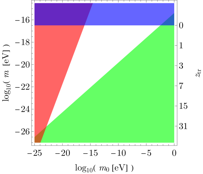
Figure 3: Dark matter mass before trapping ($m$) and after ($m_{0}$) that can explain the dark matter and dark energy of our universe, for the case of $f=10^{16}\,\mathrm{GeV}$. The allowed region is shown in white, while the colored regions are excluded from the consistency conditions of $cn<1$ (green), $\lvert\phi_{\mathrm{tr}}\rvert/f>2\pi/n$ (red), and $z_{\mathrm{tr}}>0$ (blue). The right edge of the plot shows the redshift of the trapping. For a smaller $f$, the allowed region shift towards larger values of the masses and redshift.

‘Axion’ abundance: After the trapping, the oscillating scalar can be interpreted as a collection of axion-like particles with mass $m_{0}$ and “axion decay constant” $f_{0}$ (although this is an abuse of language as in the toy model under study we do not consider any direct couplings between $\phi$ and other matter fields.) Using these quantities, the ratio of the oscillation energy to the critical density today can be written as

$$\Omega_{\mathrm{osc}}h^{2}\sim 10^{-1}\left(\frac{m_{0}}{10^{-22}\,\mathrm{eV}}\right)^{1/2}\left(\frac{f_{0}}{10^{17}\,\mathrm{GeV}}\right)^{2}\\ \times\frac{(cn^{2})^{11/4}}{(cn)^{2}}\left(\frac{\phi_{\mathrm{tr}}}{f_{0}}\right)^{-2}.$$ (9)

If the second line is ignored, this expression is exactly the same as for the traditional axion-like particles with initial field displacement $\lvert\phi_{*}\rvert\sim f_{0}$ (see, e.g., Eq. (3.10) of Kobayashi:2017jcf ). However the trapping gives rise to the second line, which is guaranteed to be larger than unity from (3) and (4). This enhancement is understood by noting that the traditional axion density starts to redshift from its initial value $m_{0}^{2}f_{0}^{2}$ when the axion begins to oscillate at $H\sim m_{0}$. On the other hand, the two-cosine scalar begins to oscillate at a later time when $H\sim m(<m_{0})$, and then after a while it gets trapped; it is at this trapping time that the oscillation energy becomes of $m_{0}^{2}f_{0}^{2}$, cf. (5). (See DAmico:2016jbm ; Jaeckel:2016qjp for related discussions in the context of monodromy dark matter.)

Inhomogeneities: Thus far we have focused on the scalar dynamics of the homogeneous background. However it is also important to consider the inhomogeneities, particularly because inflation produces scalar field fluctuations on super-horizon scales given that the scalar existed during inflation and the inflationary Hubble rate $H_{\mathrm{inf}}$ was greater than $m$. The field fluctuations give rise to isocurvature perturbations in the dark sector Linde:1985yf ; Seckel:1985tj ; Lyth:1989pb ; Kobayashi:2013nva . However we note that the existing limits on isocurvature are mainly from measurements of the cosmic microwave background (CMB), which constrains dark matter isocurvature at recombination. Hence if the trapping happens at a later time, the dark matter isocurvature at recombination was $\delta\rho_{\mathrm{DM}}/\rho_{\mathrm{DM}}\sim H_{\mathrm{inf}}/(2\pi f)$, and thus the isocurvature measured by CMB would be much smaller than what one would naively guess from the present-day decay constant $f_{0}$. This feature of the trapping, together with the enhancement of the axion abundance (9), allows axion-like particles to evade the various standard cosmological consistency relations.

We should also remark that upon trapping, the inhomogeneities may grow as the scalar oscillates along the potential with substructure Jaeckel:2016qjp , which may even lead to formation of oscillons Amin:2011hj . Moreover, the initial field fluctuation may induce the scalar to be trapped in different local minima in different patches of the universe. This would lead to formation of domain walls, which are likely to annihilate each other due to the energy density difference between the various vacua. These walls may not disappear by today, but they do not necessarily dominate the universe if the trapping happened at a low redshift. Moreover, inhomogeneous trapping gives rise to inhomogeneous dark energy. We also mention that in regions of the universe where the dark matter density is high, such as inside galaxies, the scalar may be untrapped and oscillate along the global potential, leading to dark matter properties different from those in the intergalactic space. All these features can provide smoking-gun signals of the scenario.

Conclusions: Let us then recap and summarize the broad features of this model. If we first focus on the dark matter associated with the emergent dark energy, we can see that it was lighter in the past, with density larger compared to a naive extrapolation from its present-day value. In particular if the trapping happened between recombination and today, this would give rise to apparent discrepancies between cosmological measurements using the CMB and low-redshift probes. From this point of view, it would be very interesting to study the implications of our scenario for the recent tensions in the measurements of $\sigma_{8}$ and $H_{0}$ Battye:2014qga ; Freedman:2017yms . We also note that if the initial dark matter mass was ultralight, this will have an effect on structure formation with a greater suppression of small scale structure in the past as compared to today. Dark matter becoming heavier can also shorten its lifetime, and thus may lead to enhanced signals in indirect searches. Furthermore, when viewing the dark matter as a collection of axion-like particles, we showed that naive estimates of the abundance and isocurvature modes based on the axion’s current mass and decay constant will most likely be wrong—we expect a larger abundance today, as well as a far smaller isocurvature mode arising at early times.

With regards to the dark energy, we find that it was smaller in the past. There are two possibilities that should be considered. The first is that the true, global, minimum (or minima) of the potential are exactly zero. Then, the fact that trapping minima generically occur near the global minima would naturally lead to a small cosmological constant, in the sense that the field would be accidentally caught in a wrinkle close to where $V\simeq 0$. In this picture, the question of why the dark matter and dark energy densities are of the same order today, can be rephrased as, why did the trapping happen at the right time? From this point of view, it would be important to explore microscopic realizations of the trapping to see how the trapping time is constrained in explicit models. (A multi-cosine model may be constructed using the clockwork mechanism Choi:2015fiu ; Kaplan:2015fuy .) Another possibility is that the global minima are negative and so the global vacuum structure is anti-DeSitter space. In this case, the complexity of the potential would be one way of explaining why we could live in such a universe with what is effectively a positive cosmological constant. We also note that the increasing dark energy, when averaged over time, gives rise to an equation of state $w<-1$; such a behaviour is preferred by some recent observations Shafer:2013pxa .

In this letter we have presented an intriguing possibility, that complex potential might lead to a small cosmological constant from an energy difference between its global and local minima, and that dark energy and dark matter might be intertwined. A more thorough analysis is required to check if this is truly viable, i.e. if it leads to the distances and growth rates which are consistent with current observations. We leave this for future work.

- (1) J. Martin, C. Ringeval and V. Vennin, Phys. Dark Univ. 5-6, 75 (2014) [arXiv:1303.3787 [astro-ph.CO]].
- (2) A. Arvanitaki, S. Dimopoulos, S. Dubovsky, N. Kaloper and J. March-Russell, Phys. Rev. D 81, 123530 (2010) [arXiv:0905.4720 [hep-th]].
- (3) A. Ringwald, Phys. Dark Univ. 1, 116 (2012) [arXiv:1210.5081 [hep-ph]].
- (4) D. J. E. Marsh, Phys. Rept. 643, 1 (2016) [arXiv:1510.07633 [astro-ph.CO]].
- (5) L. Hui, J. P. Ostriker, S. Tremaine and E. Witten, Phys. Rev. D 95, no. 4, 043541 (2017) [arXiv:1610.08297 [astro-ph.CO]].
- (6) E. J. Copeland, M. Sami and S. Tsujikawa, Int. J. Mod. Phys. D 15, 1753 (2006) [hep-th/0603057].
- (7) T. Clifton, P. G. Ferreira, A. Padilla and C. Skordis, Phys. Rept. 513, 1 (2012) [arXiv:1106.2476 [astro-ph.CO]].
- (8) D. Sloan and P. Ferreira, Phys. Rev. D 96, no. 4, 043527 (2017) [arXiv:1612.02853 [gr-qc]].
- (9) M. Soljacic and F. Wilczek, Phys. Rev. Lett. 84, 2285 (2000) [cond-mat/9904190].
- (10) M. R. Douglas and S. Kachru, Rev. Mod. Phys. 79, 733 (2007) [hep-th/0610102].
- (11) P. G. Ferreira, C. T. Hill and G. G. Ross, Phys. Lett. B 763, 174 (2016) [arXiv:1603.05983 [hep-th]].
- (12) P. G. Ferreira, C. T. Hill and G. G. Ross, Phys. Rev. D 95, no. 4, 043507 (2017) [arXiv:1610.09243 [hep-th]].
- (13) The second derivative of the potential is dominated by the term, i.e., . However, even during the ‘frozen’ phase, the scalar is actually slowly rolling. Therefore the time-averaged second derivative from around the onset of the oscillation is .
- (14) We should comment on the special cases where the calculations break down. If the scalar is trapped very close to the edge of the region with minima, , then the potential well is very shallow and hence becomes much smaller than the estimate of (5). On the other hand if , and further if the scalar is trapped in a local minimum that is almost degenerate with the global one, then becomes much smaller than the estimate of (6).
- (15) P. A. R. Ade et al. [Planck Collaboration], Astron. Astrophys. 594, A13 (2016) [arXiv:1502.01589 [astro-ph.CO]].
- (16) V. Iršič, M. Viel, M. G. Haehnelt, J. S. Bolton and G. D. Becker, Phys. Rev. Lett. 119, no. 3, 031302 (2017) [arXiv:1703.04683 [astro-ph.CO]].
- (17) E. Armengaud, N. Palanque-Delabrouille, C. Yèche, D. J. E. Marsh and J. Baur, Mon. Not. Roy. Astron. Soc. 471, no. 4, 4606 (2017) [arXiv:1703.09126 [astro-ph.CO]].
- (18) T. Kobayashi, R. Murgia, A. De Simone, V. Iršič and M. Viel, Phys. Rev. D 96, no. 12, 123514 (2017) [arXiv:1708.00015 [astro-ph.CO]].
- (19) S. R. Coleman and F. De Luccia, Phys. Rev. D 21, 3305 (1980).
- (20) G. D’Amico, T. Hamill and N. Kaloper, Phys. Rev. D 94, no. 10, 103526 (2016) [arXiv:1605.00996 [hep-th]].
- (21) J. Jaeckel, V. M. Mehta and L. T. Witkowski, JCAP 1701, no. 01, 036 (2017) [arXiv:1605.01367 [hep-ph]].
- (22) A. D. Linde, Phys. Lett. 158B, 375 (1985).
- (23) D. Seckel and M. S. Turner, Phys. Rev. D 32, 3178 (1985).
- (24) D. H. Lyth, Phys. Lett. B 236, 408 (1990).
- (25) T. Kobayashi, R. Kurematsu and F. Takahashi, JCAP 1309, 032 (2013) [arXiv:1304.0922 [hep-ph]].
- (26) M. A. Amin, R. Easther, H. Finkel, R. Flauger and M. P. Hertzberg, Phys. Rev. Lett. 108, 241302 (2012) [arXiv:1106.3335 [astro-ph.CO]].
- (27) R. A. Battye, T. Charnock and A. Moss, Phys. Rev. D 91, no. 10, 103508 (2015) [arXiv:1409.2769 [astro-ph.CO]].
- (28) W. L. Freedman, Nat. Astron. 1, 0169 (2017) [arXiv:1706.02739 [astro-ph.CO]].
- (29) K. Choi and S. H. Im, JHEP 1601, 149 (2016) [arXiv:1511.00132 [hep-ph]].
- (30) D. E. Kaplan and R. Rattazzi, Phys. Rev. D 93, no. 8, 085007 (2016) [arXiv:1511.01827 [hep-ph]].
- (31) D. L. Shafer and D. Huterer, Phys. Rev. D 89, no. 6, 063510 (2014) [arXiv:1312.1688 [astro-ph.CO]].