Real space mapping of topological invariants using artificial neural networks

Abstract

Topological invariants allow to characterize Hamiltonians, predicting the existence of topologically protected in-gap modes. Those invariants can be computed by tracing the evolution of the occupied wavefunctions under twisted boundary conditions. However, those procedures do not allow to calculate a topological invariant by evaluating the system locally, and thus require information about the wavefunctions in the whole system. Here we show that artificial neural networks can be trained to identify the topological order by evaluating a local projection of the density matrix. We demonstrate this for two different models, a 1-D topological superconductor and a 2-D quantum anomalous Hall state, both with spatially modulated parameters. Our neural network correctly identifies the different topological domains in real space, predicting the location of in-gap states. By combining a neural network with a calculation of the electronic states that uses the Kernel Polynomial Method, we show that the local evaluation of the invariant can be carried out by evaluating a local quantity, in particular for systems without translational symmetry consisting of tens of thousands of atoms. Our results show that supervised learning is an efficient methodology to characterize the local topology of a system.

I Introduction

The study of topological electronic phases is one of the central topics in modern Condensed Matter Physics. Depending on the symmetry class different topological states exist, with the paradigmatic examples of time reversal topological insulators,Hasan and Kane (2010) topological superconductors,Qi and Zhang (2011) topological crystal insulators,Fu (2011) topological Kondo insulatorsDzero et al. (2010) and topological Mott insulatorsRaghu et al. (2008) among others. The most fundamental quantity to characterize these states is the so called topological invariant, whose value determines the topological class of the system. In particular, interfaces between systems with different topological invariants show topologically protected excitations, resilient towards perturbations respecting the symmetry class of the system. Computationally, the calculation of the topological invariant usually requires the explicit knowledge of the wavefunctions of the entire system.Soluyanov and Vanderbilt (2011); Gresch et al. (2017); Wu et al. (2017) In particular, topological invariants can be calculated as the winding number of the occupied wave functions under twisted boundary conditions.Soluyanov and Vanderbilt (2011); Gresch et al. (2017); Wu et al. (2017) In that way, these methods generically require computing the full wavefunctions, that becomes a cumbersome task for systems without translational symmetry consisting on thousands of atoms.

In several situations of experimental relevance, translational symmetry is broken and systems are able to show different phases in real space due to the spatial modulation of the effective parameters. This situation might lead to protected modes between different regions of the system, dramatically changing the low energy properties of the whole material. This is the natural scenario in van der Waals heterostructures, where Moire patternsSan-Jose et al. (2014); Jung et al. (2017); Wang et al. (2016) could coexist with any topological state.Sanchez-Yamagishi et al. (2017); Young et al. (2014) A more controlled situation is the proposals for topological superconductivity involving nanowires, where the topological state is controlled locally by electric gates.Alicea et al. (2011); Zhang et al. (2016) Even though real space formulations for the topological invariant do exist,Bianco and Resta (2011); Marrazzo and Resta (2017); Loring (2015); Mitchell et al. (2018); Fulga et al. (2016) their computation requires an integration over the whole space. Thus, there is not a simple methodology to obtain a topological invariant in inhomogeneus systems by evaluating solely their local properties.

Application of Machine learning methods in Condensed Matter Physics is a growing area. A significant advantage of these techniques is that they are capable of finding the important degrees of freedom of a dataset without needing a profound insight of the treated problem. The identification of phase transitionsvan Nieuwenburg et al. (2017); Ch’ng et al. (2017); Ohtsuki and Ohtsuki (2016); Hu et al. (2017); Broecker et al. (2017); Koch-Janusz and Ringel (2017) and the study of the ground state and correlations in different quantum many body problemsCarleo and Troyer (2017); Deng et al. (2016, 2017); Zhang and Kim (2017); Nagai et al. (2017); Ch’ng et al. (2018) are just some of the problems that Machine Learning has helped tackle in the past few years. Even some techniques have been used in combination with ab initio calculations allowing a broader and more accurate understanding of materials.Rupp et al. (2012); Bartok et al. (2017); Gao et al. (2016) Within the language of machine learning, the calculation of topological invariants is understood as a simple classification algorithm,Zhang et al. (2018); Yoshioka et al. (2017) that could be efficiently tackled with the so called artificial neural networks. Krizhevsky et al. (2012); Dede and Sazlı (2010); Lecun et al. (1998); Goldberg (2015); Bengio et al. (2003); Schaul et al. (2010)

In this manuscript we show that artificial neural networks (ANN) are capable of characterizing the local topology of a system using as input a restricted amount of real space information. In particular, we show that a trained ANN identifies correctly the local topological character in spatially varying Hamiltonians that create topologically different regions in space. Importantly, we show that this technique, used in conjunction with the kernel polynomial method, allows to compute local topological invariants with an algorithm whose computational cost scales just linearly with the size of the system.

The rest of the paper is organized as follows. In section II we review the basics of artificial neural networks (Sec. II.1) and summarize the use of the kernel polynomial method to efficiently compute density matrices (Sec. II.2). In section III we apply the combined ANN-KPM technique both to a model Hamiltonian for a 1-D topological superconductor (Sec. III.1) and a 2-D anomalous Hall insulator (Sec. III.2). Finally, in section IV we present our conclusions.

II Method

II.1 Artificial Neural Networks

Machine Learning (ML) is a broad field that includes many different approaches, goals and methods.Solomonoff (1957) The defining property of ML algorithms is that they allow computers to perform specific tasks without being explicitly programmed for each one of them.Samuel (1959) Within the vast variety of ML algorithms, we will focus on supervised learning algorithms, which require a training dataset to fit the parameters in the model. One of the most common models of supervised learning are Artificial Neural Networks (ANN) which have been proven very useful to model patterns and correlations of complex problems that cannot be modeled analytically such as image or sound recognition,Krizhevsky et al. (2012); Dede and Sazlı (2010); Lecun et al. (1998) and even natural language processing.Goldberg (2015); Bengio et al. (2003) In our case, we aim to use an artificial neural network to characterize locally the topological state of a one (Fig. 1 (a)) or two (Fig. 1 (b)) dimensional system. The objective of the procedure is to have a neural network that, given local information about the system, returns the topological invariant as sketched in Fig. 1 (c). The local information that will be provided is a local block of the density matrix of the system, as we will discuss later.

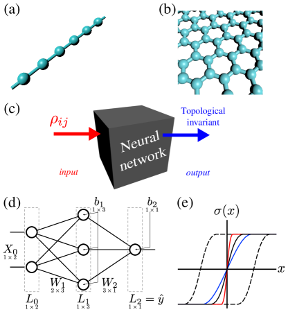
Figure 1: Panels (a,b) show a cartoon of the two different geometries of the model Hamiltonians considered below, a one dimensional topological superconductor (a) and a two dimensional quantum anomalous Hall insulator (b). Panel (c) shows a schematic sketch of our procedure: a trained neural network will take as input a local density matrix, and it will return the topological invariant of the system. Panel (d) shows a sketch for an artificial neural network as described in the text, whereas in (e) we sketch the standard behavior of an activation function of a neuron, $\sigma(x)$, for different weights (colors) and bias (dashed lines).

ANN are loosely based on parts of the brain, consisting of neurons, modeled as perceptronsRosenblatt (1958), and synapses as shown in Fig. 1 (a). The neurons in an ANN do not attempt to model the actual structure or behavior of the biological cellsHodgkin and Huxley (1952). Instead, they mimic one of their main features, the activation function. This activation function, $\sigma$, sketched in Fig. 1 (b) provides the output of each neuron based on the received inputs and an external parameter (bias). For computational convenience, $\sigma$ should be any smooth and differentiable function defined over $\mathbb{R}$ but with its range restricted to a closed interval, namely $\sigma\in[-1,1]$, as depicted in Fig. 1 (e). Usually, these functions are either the $\tanh$ or the sigmoid function, but others might be used without loss of generality or functionality since these models are only weakly sensitive to these details.Hopfield (1982)

The inputs $X$ entering each neuron are weighted by the synapses $W$ and shifted by the bias $b$. The synapses’ weights are parameters to be tuned and they can be arranged as rectangular matrices, $W^{\alpha}$, so the output $L$ of the layer $\alpha$ can be obtained simply as: $L_{\alpha}=\sigma(X_{\alpha}\cdot W_{\alpha}+b_{\alpha})$, where $X_{\alpha}$ is the input of the layer $\alpha$ (note that for the hidden layers $X_{\alpha}=L_{\alpha-1}$). As a formative example the outputs of every layer of the toy model sketched in Fig. 1 (d) can be calculated as follows:

$$\begin{split}L_{0}&=\sigma(X_{0})\quad\text{or just}\quad L_{0}=X_{0}\\ L_{1}&=\sigma\left(L_{0}\cdot W_{1}+b_{1}\right)\\ L_{2}&=\sigma\left(L_{1}\cdot W_{2}+b_{2}\right)=\hat{y}\end{split}$$ (1)

where $X_{0}$ is the input fed to the ANN. The matrices $W_{\alpha}$ and the arrays $b_{\alpha}$ are the parameters to be fitted during the training process in order to modify the activation functions of each of the neurons in the ways showed in Fig. 1 (e). Note that the number of parameters in ANN models grows very quickly with the size (number of neurons per layer) and depth (number of layers) of the network.

Artificial neural network, as every supervised learning algorithm, consist in three phases. First, the architecture of the model (i.e. the number of layers and neurons per layer) is decided depending on the complexity of the problem addressed. Second, the model is trained. In this process, several input-output pairs are provided to the model whose parameters are fitted to mimic the correlations present in the user-provided data. Finally, when the training is completed, the model can be used to evaluate new (unseen) input data.

Supervised learning algorithms require a training dataset to optimize the parameters of the models. The training is performed by minimizing a cost function, $\mathcal{E}$, usually proportional to the squared difference between the expected output, $y$, and the actual output of the network, $\hat{y}$.

$$\mathcal{E}=\tfrac{1}{2}(y-\hat{y})^{2}$$ (2)

Notice that $y$ is a constant defined by the (user-provided) training dataset while $\hat{y}$ depends on all the parameters of the network (weights and bias). The minimization of $\mathcal{E}$ is, then, performed by iteratively modifying the values of all the weights and bias in the network until the desired output is obtained. This is a computationally complex and expensive process since the number of parameters can range from a few tens to millions. In fact, it was not until 1986 that an efficient method was developed for such a purpose.Rumelhart et al. (1986) We use the gradient descent with the back-propagation algorithm to train the ANN, which is the most common approach nowadays. We used the open source library PyBrain,Schaul et al. (2010) to create, train and evaluate the ANN.

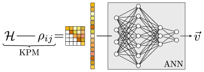
Figure 2: Sketch of the process to evaluate the topological character of a local region of space. The density matrix corresponding to a certain area in space is calculated using the KPM, after removing the redundant elements the matrix is rearranged in a 1D array that is used as input for neural network that will provide the corresponding topological invariant as output.

II.2 Correlation functions with the Kernel Polynomial method

In this section we review how real space correlation functions can be efficiently calculated using the Kernel polynomial method (KPM).Weiße et al. (2006) We will focus the discussion in the case of a normal electronic system, since the case of a superconductor can be treated in an analogous way. The main task that we have to perform is to obtain the density matrix, evaluated in a restricted area of real space, of a certain (very large) Hamiltonian. In terms of the eigenfunctions $|\Psi_{k}\rangle$ of the Hamiltonian $H$, the elements of the density matrix can be written as

$$\rho_{ij}=\int_{-\infty}^{E_{F}}\langle i|\Psi_{k}\rangle\langle\Psi_{k}|j\rangle\delta(E_{k}-\omega)d\omega$$ (3)

where $|i\rangle$ and $|j\rangle$ are the elements of the basis for the Hamiltonian $H$ and $E_{F}$ is the Fermi energy. The diagonal elements of the matrix, $\rho_{ii}$, are the integrated local density of states. In the gapped state, the off-diagonal elements are expected to decay exponentially with distance. So, when the Fermi energy $E_{F}$ lies in the gap, the density matrix is properly described by restricting the calculation to a set of neighboring sites. Generically, calculating the previous matrix requires diagonalizing the full Hamiltonian to obtain the occupied wavefunctions, a task that scales with $\mathcal{O}(N^{3})$, with $N$ the system size of the system. The Kernel Polynomial Method allows the computation of $\rho_{ij}$, for a restricted set of neighboring sites, with a computational cost that scales only as $\mathcal{O}(N)$.

The KPM allows to compute the quantity

$$g_{ij}(\omega)=\sum_{k}\langle i|\Psi_{k}\rangle\langle\Psi_{k}|j\rangle\delta(E_{k}-\omega)$$ (4)

which can easily be integrated to obtain the density matrix (3). The central idea is that $g_{ij}$ can be expressed in matrix form as

$$g_{ij}(\omega)=\langle i|\delta(H-\omega)|j\rangle$$ (5)

The KPM consists on expanding equation (5) in terms of Chebyshev polynomials $T_{n}(\omega)$. To do so, the Hamiltonian is first rescaled so that all the eigenenergies lie in the interval $\mathcal{E}_{k}\in(-1,1)$. The rescaled Hamiltonian is denoted as $\mathcal{H}$. The corresponding spectral function is calculated as

$$g_{ij}({\omega})=\frac{1}{\pi\sqrt{1-\omega^{2}}}\left(\bar{\mu}_{n}+2\sum^{N}_{n=1}\tilde{\mu}_{n}T_{n}(\bar{\omega})\right)$$ (6)

The coefficients $\tilde{\mu}_{n}$ determine the expansion of a certain element $g_{ij}$, and are calculated as

$$\tilde{\mu}_{n}=g^{N}_{n}\mu_{n}$$ (7)

where $\mu_{n}$ are the coefficients calculated from the Hamiltonian $\mathcal{H}$ and $g_{n}^{N}$ denotes the Jackson Kernel that improves the convergence of the seriesWeiße et al. (2006)

$$g_{n}^{N}=\frac{(N-n-1)\cos\frac{\pi n}{N+1}+\sin\frac{\pi n}{N+1}\cot\frac{\pi}{N+1}}{N+1}$$ (8)

Given two sites $i$ and $j$, we define two vectors located in those sites $v_{i}$ and $v_{j}$. The coefficients $\mu_{n}$ would be calculated as a conventional functional expansion

$$\mu_{n}=\langle v_{i}|\int_{-1}^{1}\delta(\mathcal{H}-\omega)T_{n}(\mathcal{H})d\omega|v_{j}\rangle$$ (9)

which in the diagonal basis reads

$$\mu_{n}=\int_{-1}^{1}\langle v_{i}|\Psi_{k}\rangle\delta(\mathcal{E}_{k}-\omega)\langle\Psi_{k}|v_{j}\rangle T_{n}(\omega)d\omega$$ (10)

Performing the integration over $\omega$ we get

$$\mu_{n}=\langle v_{i}|\Psi_{k}\rangle T_{n}(\mathcal{E}_{k})\langle\Psi_{k}|v_{j}\rangle=\langle v_{i}|T_{n}(\mathcal{H})|v_{j}\rangle$$ (11)

Therefore, the coefficients $\mu_{n}$ can be calculated as the overlap of two vectors

$$\mu_{n}=\langle v_{j}|\alpha_{n}\rangle$$ (12)

where $\alpha_{n}$ is calculated with the recursion relations associated to the Chebyshev polynomials

$$|\alpha_{0}\rangle=|v_{i}\rangle$$ (13)

$$|\alpha_{1}\rangle=\mathcal{H}|\alpha_{0}\rangle$$

$$|\alpha_{n+1}\rangle=2\mathcal{H}|\alpha_{n}\rangle-|\alpha_{n-1}\rangle$$

This procedure thus involves matrix vector products to calculate the coefficients. For a sparse matrix, as it is the case of a tight binding Hamiltonian, the number of non-zero elements scales linearly with the system size, so the computational cost of calculating the density matrix for a fixed number of sites also scales linearly. This method allows to compute $g_{ij}$ at every energy simultaneously, so that $\rho_{ij}$ can be calculated by integration up to the Fermi energy.

For small systems, the density matrix can be calculated also by exact diagonalization of the full Hamiltonian. In principle, that procedure allows to calculate the correlation function of relatively large one dimensional systems. However, for a two dimensional system, the dimension of the matrix will be too large in general. It is in that situation when the kernel polynomial method is specially suitable.

III Topological invariants with supervised learning

We now describe the procedure to characterize the local topological character of a system using ANN. We choose as input the elements of the density matrix that involve one site and its closest neighbors. This procedure allows to naturally treat systems without translation symmetry and with disorder, as the calculation of the density matrices is not more computationally expensive in those situations using the previous procedure. The process to calculate the density matrix was discussed in Sec. II.2 but in order to use the density matrix as input for our ANN some processing is required. The density matrix is, in general, a complex Hermitian matrix, so we will remove the redundant elements (namely the lower triangle) and arrange the remaining elements in a 1D array, concatenating the real and imaginary parts. Furthermore, we included the eigenvalues of the density matrix as part of the input. Strictly, the inclusion of the eigenvalues is a redundant operation that could be avoided by increasing the size and/or depth of the ANN, yet we found that it helped the optimization of the model with a negligible computational overhead. The output of the NN will be the topological invariant of the system. The calculation of the corresponding output is done by constructing a translational invariant Hamiltonian in which the corresponding topological invariant is well defined and can be calculated in a standard way. Finally, since we are using the ANN as a classifier, it is convenient to encode the possible outputs as linearly independent vectors, $\vec{v}$, rather than use a single scalar. The use of vectors allows the discrimination between wrong answers and false positives. This whole architecture is sketched in Fig. 2.

In order to train of the ANN we generate a large number of realizations of a family of Hamiltonians, exploring their parameter space. For a given choice of parameters, we compute the topological invariant of the corresponding pristine case and its local density matrix. These procedure allows us to generate a set of inputs and outputs, which are used to train the NN. Once the ANN is trained, the model is ready to be evaluated with new data that the network has never tried to test the accuracy of the network. The last step is to create a new Hamiltonian with spatially dependent parameters, and evaluate the NN with the local density matrix corresponding to a neighborhood of every lattice site. In this way, we have a procedure to locally evaluate the topological invariant of a systems lacking translational symmetry.

III.1 One dimensional topological superconductor

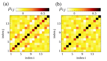
Figure 3: Image representation of the density matrix for two particular different states for the superconducting 1D system, trivial (a) and topological (b). In terms of the matrices shown, the task of the neural network can be understood as an image recognition algorithm capable of distinguishing an input (a) from (b), for different parameters of the Hamiltonian chosen randomly. The different indexes in x and y axis run over spin and electron/hole sectors in the closest sites.

In the following, we will consider a lattice model Hamiltonian for a one dimensional electron gas that is able to host both trivial and topological superconducting states. The corresponding topological invariant is a $Z_{2}$ number that can be calculated as a Berry phase.Budich and Ardonne (2013) Such effective one dimensional system, in particular the superconducting topological phase, is realized in semiconducting nanowires deposited on top of a s-wave superconductor.Lutchyn et al. (2010); Oreg et al. (2010); Mourik et al. (2012); Stanescu et al. (2011); Lutchyn et al. (2011, 2017); Aguado (2017) The model describes electrons in a 1D chain, in the presence of Zeeman field, Rashba spin-orbit coupling, superconducting proximity effect and a sublattice imbalance term. Thus, the model has six different parameters: a spin-conserving hopping $t$, chemical potential $\mu$, Rashba spin orbit $t_{R}$, external Zeeman field $B_{z}$, on-site pairing term $\Delta$ and a trivial mass $m$. Moreover, we also include the possibility of having finite Anderson disorder $W_{i}$, so that the full Hamiltonian reads

$$\begin{split}\mathcal{H}=&-t\sum_{\langle ij\rangle_{\alpha}}c^{\dagger}_{i\alpha}c_{j\alpha}+it_{R}\sum_{\langle ij\rangle_{\alpha\beta}}\hat{e}_{z}\cdot(\vec{\sigma}_{\alpha\beta}\times\vec{d}_{ij})c^{\dagger}_{i\alpha}c_{j\beta}\\ &+B_{z}\sum_{i\alpha}c^{\dagger}_{i\alpha}\sigma_{z}c_{i\alpha}+\Delta\sum_{i}[c_{i\uparrow}c_{i\downarrow}+c^{\dagger}_{i\downarrow}c^{\dagger}_{i\uparrow}]\\ &+\mu\sum_{i,\alpha}c^{\dagger}_{i\alpha}c_{i\alpha}+m\sum_{i}\tau_{i}c^{\dagger}_{i}c_{i}+\sum_{i,\alpha}W_{i}c^{\dagger}_{i\alpha}c_{i\alpha}\end{split}$$ (14)

The previous Hamiltonian can have topological and trivial phases. In a nutshell, a topological phase may arise when the Zeeman term $B_{z}$ is such that the chemical potential $\mu$ crosses only one of the spin channels, so that a small pairing $\Delta$ and Rashba field $t_{R}$ gives rise to a spinless p-wave superconductor.Lutchyn et al. (2011) In the absence of both Zeeman and Rashba couplings, the induced superconducting gap is trivial.

The Hamiltonian (14) is solved in the Nambu representation by defining a spinor wavefunction as $\Psi^{\dagger}=\begin{pmatrix}c^{\dagger}_{\uparrow},&c^{\dagger}_{\downarrow},&c_{\downarrow},&-c_{\uparrow}\end{pmatrix}$ which gives rise to a Bogoliuvov-de-Gennes Hamiltonian $\mathcal{H}=\frac{1}{2}\Psi^{\dagger}H\Psi$. The matrix $H$ is used to calculate the correlation functions $\langle c_{i,s}c_{j,s^{\prime}}\rangle$ and $\langle c^{\dagger}_{i,s}c_{j,s^{\prime}}\rangle$, as introduced in section II.2, by integrating the different $g_{ij}(\omega)$ from $\omega=-\infty$ up to $\omega=0$. In Fig. 3 we show an example of two different input data from the training dataset, for a topological (a) and a trivial (b) state computed for an open chain with $N=400$ sites using the KPM. It is evident that simple inspection is not enough to distinguish between the two of them.

In order to generate the training dataset we considered different Hamiltonians for a bipartite chain with 400 sites by varying the different values for the off-plane Zeeman field $B_{z}$, Rashba $\lambda_{R}$, chemical potential $\mu$, superconducting pairing $\Delta$ and sublattice imbalance $m$. In order to prove the robustness of our procedure, we also switch on the Anderson on-site disorder ($W\in(0.0,0.4t)$), with a magnitude comparable to the other energy scales. For the training dataset we generated 1000 different Hamiltonians with parameters randomly chosen in the following ranges: $t_{R}\in[-0.3t,0]$, $B_{z}\in[0.2t,0.8t]$, $\mu\in[t,2t]$, $\Delta\in[0.1t,0.3t]$, $m\in[-0.2t,0.2t]$, yielding a five dimensional phase space. Using the generated Hamiltonians we calculate the density matrix of the central atom in the nanowire, $\rho_{ij}$, and its three closest neighbors. Since the Hamiltonian in eq. (14) only involves two Pauli matrices for a linear chain, the Hamiltonian in real space can be chosen to be purely real, so that its density matrix will be also real. For each example the $Z_{2}$ topological invariant is calculated for the pristine system ($W_{i}=0$) defined by that particular set of parameters, which is used as expected output. Since this topological invariant only has two possibilities, we encode the $Z_{2}$ invariant as a two dimensional vector $v$, so that the topological case corresponds to $v=(1,0)$ and the trivial case to $v=(0,1)$. With this methodology a single element of the training dataset has a 152-dimensional input and a 2-dimensional output. We took two hidden layers with 101 and 21 neurons. After training, a validation set with 200 new samples is generated to test the accuracy of the ANN yielding an accuracy of $\sim 97\%$. In order to gain some insight on the ANN capabilities, we run a simple test by freezing all the parameters in the Hamiltonian (14) but the chemical potential and comparing the actual $Z_{2}$ with the output provided by the ANN. In Fig 4 (a) we see that even for unseen data the NN is able to provide the correct topological invariant.

Once the network is trained, it is ready to be used in the case of an inhomogeneus system. We now generate a one dimensional system following equation (14) with spatially varying couplings. In particular, we modulate the chemical potential along the chain as shown in Fig. 4 (b). Such modulation is feasible by means of local gates in the experimental realizations involving semiconducting nanowires.Zhang et al. (2016) With such modulation, we observe the emergence of zero energy modes in the local density of states 4 (c), which are expected to be a signature of a boundary between a trivial and topological phase. The evaluation of the topological invariant on every atomic position of the chain can be carried out by feeding the local density matrix to the trained neural network. Our network shows that the different regions of the space have different topological invariants as shown in Fig. 4 (d). It is observed that the points of space where the topological invariant changes in Fig. 4 (d) correspond to the location of the zero energy Majorana modes, as seen in Fig. 4 (c), validating the performance of our neural network.

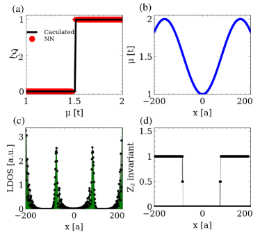
Figure 4: (a) Comparison of the topological invariant computed exactly with the one predicted by the trained neural network in a pristine system, showing that the ANN perfectly captures the phase transitions in the homogeneus system. Afterwards, we create a inhomogeneus system with modulated chemical potential as shown in panel (b). Such modulation creates trivial and topological zones, with Majorana modes pinned at the transition points (c). The neural network is then evaluated in every point of the space, yielding a site-dependent topological invariant shown in (d). The topological transitions shown in (d) mark the existence of zero Majorana modes obtained in (c). The parameters used are $\lambda_{R}=-0.3t$ $B_{z}=0.5t$, $m=0$, and $\Delta=0.1t$.

The success of the neural network in describing the topological order of the different phases implies that, locally, the density matrix carries enough information to distinguish between the two cases. In particular, the elements of $\rho_{ij}$ involving $\langle c_{i,s}c_{j,s^{\prime}}\rangle$ encode information about the induced superconducting order parameter, both in the $s$ and $p$-wave channels, which physically is expected to determine the topological phase. If, in comparison, only the diagonal part of the density matrix was used as input for the neural network, it would not be possible to distinguish between trivial and topological states. This is easily understood taking into account that the diagonal part of $\rho_{ij}$ accounts for the total occupation numbers and two topologically inequivalent band-structures can have arbitrarily similar density of states.

III.2 Two dimensional Chern insulator

In this section we will use an analogous methodology to study a topological two dimensional state. In particular, we consider a model Hamiltonian for electrons moving in a honeycomb lattice with Rashba spin orbit coupling $t_{R}$, off-plane exchange $B_{z}$, that is known to result in a two dimensional Quantum Anomalous Hall state (QAH)Qiao et al. (2010):

$$\begin{array}[]{c@{}l}H=-t\sum_{\langle ij\rangle_{\alpha}}c^{\dagger}_{i\alpha}c_{j\alpha}+it_{R}\sum_{\langle ij\rangle_{\alpha\beta}}\hat{e}_{z}\cdot(\vec{\sigma}_{\alpha\beta}\times\vec{d}_{ij})c^{\dagger}_{i\alpha}c_{j\beta}\\ +B_{z}\sum_{i\alpha}c^{\dagger}_{i\alpha}\sigma_{z}c_{i\alpha}+m\sum_{i,\alpha}\tau_{i}c^{\dagger}_{i\alpha}c_{i\alpha}\\ +\sum_{i,\alpha}W_{i}c^{\dagger}_{i\alpha}c_{i\alpha}\end{array}$$ (15)

where $t_{R}$ is the Rashba coupling, $\vec{\sigma}$ are the spin Pauli matrices, $B_{z}$ is the external Zeeman field and $\tau_{i}=\pm 1$ is the sublattice operator. The first term is the usual tight-binding hopping term, the second one describes the Rashba interaction Qiao et al. (2010); Min et al. (2006) and the third term is the so-called exchange or Zeeman term which couples to the spin degree of freedom. The fourth term is a trivial mass term that assigns an opposite on-site energy for the atoms in each of the sublattices, that we introduce in order to have a trivial insulator phase in the model. Finally, the last term is an Anderson disorder term that we introduce to prove the robustness of the procedure. For $m=0$, and $B_{z}\neq 0$ and $t_{R}\neq 0$, the model has a topological gap with a with Chern number $\mathcal{C}=\pm 2$. For $m\neq 0$ and $B_{z}=0$. the model has a trivial ($\mathcal{C}=0$) gap.

Each of these Hamiltonian terms can effectively describe different experimental situations. The sublattice imbalance could arise for a graphene monolayer deposited on boron nitride in a commensurate fashion.Wang et al. (2016); Lado et al. (2013) The Rashba and exchange fields naturally arise for a graphene monolayer deposited over a ferromagnetic insulator, such as YIG,Tang et al. (2017); Wang et al. (2015) EuOSu et al. (2017) or CrI₃.Huang et al. (2017); Zhang et al. (2017) Furthermore, the non commensuration of graphene with the substrate creates Moire patterns, resulting in an effective spatial modulation of the different contributions.San-Jose et al. (2014); Jung et al. (2017); Wang et al. (2016)

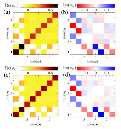
Figure 5: Real and imaginary parts of the density matrix for a trivial $\mathcal{C}=0$ (a,b) and a topological $\mathcal{C}=2$ (c,d) two dimensional system. In this case, the neural network will implement an image recognition algorithm, where the input are the two images representing the real and imaginary parts.

It is worth mentioning two important differences with respect to the model presented in Sec. III.1. On one hand, now the Hamiltonian involves the three Pauli matrices, so in general it will be complex. This implies that the calculated density matrices will also be complex, so that the neural network will receive as input both the real and imaginary components. On the other hand, since we are dealing now with a two dimensional system, a finite island will have $L^{2}$ sites, with $L$ the typical size of the island. In particular, the calculation of a the density matrix with the wavefunctions of an island with side $L\approx 300$ would require the diagonalization of matrix of dimension $L^{2}\approx 90000$, whose computational complexity is $L^{6}$. It is in this situation where the KPM will be specially useful, as it allows us to calculate the density matrix with a computational complexity of the number of sites, $L^{2}$.

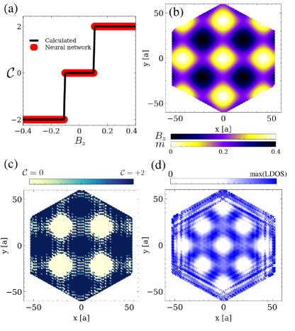
Figure 6: (a) Comparison between the exact Chern number (black) and the prediction of the trained neural network (red) using as input the local density matrix. Once the accuracy of the network has been checked, we created a big graphene island with modulated mass and exchange term as shown in (b). The neural network is used to evaluate the topological invariant in each atom, yielding the result shown in (c). The boundary between different topological phases is expected to give rise to in-gap states, which is confirmed by calculating the in-gap spectral function as shown in (d).

We now move to apply our methodology to the system defined by eq. (15). First, to train the neural network, we generate different spatially uniform Hamiltonians by choosing randomly each of the coupling parameters. The Zeeman and Rashba were randomly generated in the interval $t_{R}\in[-0.4t,0.4t]$ and the mass between $m\in[0,0.4t]$. Again, random Anderson-like disorder comparable to the other interactions are introduced all across the system $W_{i}\in[0.0,0.4t]$. The training dataset consisted in 564 samples. For every set of parameters, we built the Hamiltonian as in eq. (15) and calculated the local density matrix for the central atom and its three first neighbors which are used as input of the network, in this case a 128-dimensional array. Again we chose having two hidden layers with 101 and 21 neurons. It is worth considering again the challenging task of distinguishing between different inputs as those shown in Fig. 5, which highlights that the classification of topological and trivial phases based only in local properties is far from being a trivial task.

The output for each input was obtained by calculating the Chern number of the ground state of the system integrating the Berry curvature in the Brillouin zone of a translational invariant ($W_{i}=0$) Hamiltonian with the same parameters. Once the network was trained, we tested its accuracy on a validation dataset with 586 samples randomly generated, showing an accuracy of $\sim 92\%$. The comparison of the result predicted by the network and the one calculated exactly in a system with translational invariance is shown in Fig. 6 (a) for the different topological phases.

After the training, we generated a graphene nano-island with 7400 atoms. In this island, we choose a spatially modulated exchange field of the form $B_{z}(x,y)=0.1t[\cos(0.15x)+\cos(0.15y)+2]$, a modulated mass term of the form $m(x,y)=0.1t[\sin(0.15x)+\sin(0.15y)+2]$ (shown in Fig. 6 (b)), and a constant Rashba coupling $\lambda_{R}=0.2$. The previous modulations are expected to create neighboring trivial and topological areas depending on which is the dominant contribution, mass or exchange and Rashba couplings. With such a Hamiltonian, we calculated the local density matrix using the Kernel polynomial method, that was used as input of the neural network. The result of the evaluation of the neural network across the sample is shown in Fig. 6 (c). It can be seen that different regions with different Chern number appear according to the spatial modulation of the Hamiltonian parameters. The significance of the different regions becomes clear once the in-gap density of states is calculated in Fig. 6 (d). This shows both in-gap modes precisely at the boundary between different regions, as expected form the bulk-boundary correspondence, as well as edge states all around the sample.

This result highlights that the artificial neural network faithfully distinguishes between the different phases based solely in local information, providing an useful method to calculate the topological invariant in systems without translational symmetry.

IV Conclusions

We have shown that an artificial neural network is capable of predicting the topological nature of different model Hamiltonians using as an input a local sector of the density matrix, i.e., evaluating solely local properties. Our procedure consisted on training an artificial neural network using as input the subspace of the density matrix corresponding to a local area of the sample, and as output the topological invariant that an analogous (pristine and translational invariant) Hamiltonian with the same effective parameters would have.

We applied this procedure to two well known models, a 1D topological superconductor and 2D topological insulator. In both cases we considered finite systems with a space dependent Hamiltonian that create regions with both topological and trivial character. By evaluating the network with local quantities for each Hamiltonian we showed that the different topological domains are accurately identified by the network, even when the inhomogeneus systems have Anderson-like disorder, proving that this methodology can be applied for disordered systems.

It is worth remarking that the training procedure is carried out for a specific model, and tested in that same model for different parameters, including local modulations in space. An open question is whether this methodology can be extended to cases with the same topological classes but different geometries. Finally, it is interesting to note that an analogous methodology could be applied to interacting systems, so that similar procedures could be exploited to identify quantum spin liquid states in two dimensional spin systems.

References

- Hasan and Kane (2010) M. Z. Hasan and C. L. Kane, Rev. Mod. Phys. 82, 3045 (2010).
- Qi and Zhang (2011) X.-L. Qi and S.-C. Zhang, Rev. Mod. Phys. 83, 1057 (2011).
- Fu (2011) L. Fu, Phys. Rev. Lett. 106, 106802 (2011).
- Dzero et al. (2010) M. Dzero, K. Sun, V. Galitski, and P. Coleman, Phys. Rev. Lett. 104, 106408 (2010).
- Raghu et al. (2008) S. Raghu, X.-L. Qi, C. Honerkamp, and S.-C. Zhang, Phys. Rev. Lett. 100, 156401 (2008).
- Soluyanov and Vanderbilt (2011) A. A. Soluyanov and D. Vanderbilt, Phys. Rev. B 83, 235401 (2011).
- Gresch et al. (2017) D. Gresch, G. Autès, O. V. Yazyev, M. Troyer, D. Vanderbilt, B. A. Bernevig, and A. A. Soluyanov, Phys. Rev. B 95, 075146 (2017).
- Wu et al. (2017) Q. Wu, S. Zhang, H.-F. Song, M. Troyer, and A. A. Soluyanov, arXiv preprint arXiv:1703.07789 (2017).
- San-Jose et al. (2014) P. San-Jose, A. Gutiérrez-Rubio, M. Sturla, and F. Guinea, Phys. Rev. B 90, 075428 (2014).
- Jung et al. (2017) J. Jung, E. Laksono, A. M. DaSilva, A. H. MacDonald, M. Mucha-Kruczyński, and S. Adam, Phys. Rev. B 96, 085442 (2017).
- Wang et al. (2016) E. Wang, X. Lu, S. Ding, W. Yao, M. Yan, G. Wan, K. Deng, S. Wang, G. Chen, L. Ma, et al., Nature Physics 12, 1111 (2016).
- Sanchez-Yamagishi et al. (2017) J. D. Sanchez-Yamagishi, J. Y. Luo, A. F. Young, B. M. Hunt, K. Watanabe, T. Taniguchi, R. C. Ashoori, and P. Jarillo-Herrero, Nature nanotechnology 12, 118 (2017).
- Young et al. (2014) A. F. Young, J. D. Sanchez-Yamagishi, B. Hunt, S. H. Choi, K. Watanabe, T. Taniguchi, R. C. Ashoori, and P. Jarillo-Herrero, Nature 505, 528 (2014), letter.
- Alicea et al. (2011) J. Alicea, Y. Oreg, G. Refael, F. von Oppen, and M. P. A. Fisher, 7, 412 EP (2011), article.
- Zhang et al. (2016) H. Zhang, Ö. Gül, S. Conesa-Boj, K. Zuo, V. Mourik, F. K. de Vries, J. van Veen, D. J. van Woerkom, M. P. Nowak, M. Wimmer, et al., arXiv preprint arXiv:1603.04069 (2016).
- Bianco and Resta (2011) R. Bianco and R. Resta, Phys. Rev. B 84, 241106 (2011).
- Marrazzo and Resta (2017) A. Marrazzo and R. Resta, Phys. Rev. B 95, 121114 (2017).
- Loring (2015) T. A. Loring, Annals of Physics 356, 383 (2015).
- Mitchell et al. (2018) N. P. Mitchell, L. M. Nash, D. Hexner, A. M. Turner, and W. T. Irvine, Nature Physics , 1 (2018).
- Fulga et al. (2016) I. C. Fulga, D. I. Pikulin, and T. A. Loring, Physical review letters 116, 257002 (2016).
- van Nieuwenburg et al. (2017) E. van Nieuwenburg, Y.-H. Liu, and S. Huber, Nature Physics 13, 435 (2017), arXiv:1610.02048 .
- Ch’ng et al. (2017) K. Ch’ng, J. Carrasquilla, R. G. Melko, and E. Khatami, Phys. Rev. X 7, 031038 (2017).
- Ohtsuki and Ohtsuki (2016) T. Ohtsuki and T. Ohtsuki, Journal of the Physical Society of Japan 85, 123706 (2016).
- Hu et al. (2017) W. Hu, R. R. P. Singh, and R. T. Scalettar, Phys. Rev. E 95, 062122 (2017).
- Broecker et al. (2017) P. Broecker, F. F. Assaad, and S. Trebst, arXiv preprint arXiv:1707.00663 (2017).
- Koch-Janusz and Ringel (2017) M. Koch-Janusz and Z. Ringel, arXiv preprint arXiv:1704.06279 (2017).
- Carleo and Troyer (2017) G. Carleo and M. Troyer, Science 355, 602 (2017).
- Deng et al. (2016) D.-L. Deng, X. Li, and S. D. Sarma, arXiv preprint arXiv:1609.09060 (2016).
- Deng et al. (2017) D.-L. Deng, X. Li, and S. Das Sarma, Phys. Rev. X 7, 021021 (2017).
- Zhang and Kim (2017) Y. Zhang and E.-A. Kim, Phys. Rev. Lett. 118, 216401 (2017).
- Nagai et al. (2017) Y. Nagai, H. Shen, Y. Qi, J. Liu, and L. Fu, Phys. Rev. B 96, 161102 (2017).
- Ch’ng et al. (2018) K. Ch’ng, N. Vazquez, and E. Khatami, Phys. Rev. E 97, 013306 (2018).
- Rupp et al. (2012) M. Rupp, A. Tkatchenko, K.-R. Müller, and O. A. von Lilienfeld, Phys. Rev. Lett. 108, 058301 (2012).
- Bartok et al. (2017) A. P. Bartok, S. De, C. Poelking, N. Bernstein, J. Kermode, G. Csanyi, and M. Ceriotti, arXiv preprint arXiv:1706.00179 (2017).
- Gao et al. (2016) T. Gao, H. Li, W. Li, L. Li, C. Fang, H. Li, L. Hu, Y. Lu, and Z.-M. Su, Journal of cheminformatics 8, 24 (2016).
- Zhang et al. (2018) P. Zhang, H. Shen, and H. Zhai, Phys. Rev. Lett. 120, 066401 (2018).
- Yoshioka et al. (2017) N. Yoshioka, Y. Akagi, and H. Katsura, arXiv preprint arXiv:1709.05790 (2017).
- Krizhevsky et al. (2012) A. Krizhevsky, I. Sutskever, and G. E. Hinton, in Advances in Neural Information Processing Systems 25 (2012) pp. 1097–1105.
- Dede and Sazlı (2010) G. Dede and M. H. Sazlı, Digital Signal Processing 20, 763 (2010).
- Lecun et al. (1998) Y. Lecun, L. Bottou, Y. Bengio, and P. Haffner, Proc. IEEE 86, 2278 (1998).
- Goldberg (2015) Y. Goldberg, arXiv (2015), arXiv:1510.00726v1 .
- Bengio et al. (2003) Y. Bengio, R. Ducharme, P. Vincent, and C. Janvin, J. Mach. Learn. Res. 3, 1137 (2003).
- Schaul et al. (2010) T. Schaul, J. Bayer, D. Wierstra, Y. Sun, M. Felder, F. Sehnke, T. Rückstieß, and J. Schmidhuber, Journal of Machine Learning Research 11, 743 (2010).
- Solomonoff (1957) R. Solomonoff, IRE Convention Record 2, 56 (1957).
- Samuel (1959) A. L. Samuel, IBM Journal of Research and Development 3, 206 (1959).
- Rosenblatt (1958) F. Rosenblatt, Psychological Review 65, 386 (1958).
- Hodgkin and Huxley (1952) A. L. Hodgkin and A. F. Huxley, J. Physiol. 117, 500 (1952).
- Hopfield (1982) J. J. Hopfield, PNAS 79, 2554 (1982).
- Rumelhart et al. (1986) D. E. Rumelhart, G. E. Hinton, and R. J. Williams, Nature 323, 533 (1986).
- Weiße et al. (2006) A. Weiße, G. Wellein, A. Alvermann, and H. Fehske, Rev. Mod. Phys. 78, 275 (2006).
- Budich and Ardonne (2013) J. C. Budich and E. Ardonne, Phys. Rev. B 88, 075419 (2013).
- Lutchyn et al. (2010) R. M. Lutchyn, J. D. Sau, and S. Das Sarma, Phys. Rev. Lett. 105, 077001 (2010).
- Oreg et al. (2010) Y. Oreg, G. Refael, and F. von Oppen, Phys. Rev. Lett. 105, 177002 (2010).
- Mourik et al. (2012) V. Mourik, K. Zuo, S. M. Frolov, S. Plissard, E. Bakkers, and L. P. Kouwenhoven, Science 336, 1003 (2012).
- Stanescu et al. (2011) T. D. Stanescu, R. M. Lutchyn, and S. Das Sarma, Phys. Rev. B 84, 144522 (2011).
- Lutchyn et al. (2011) R. M. Lutchyn, T. D. Stanescu, and S. Das Sarma, Phys. Rev. Lett. 106, 127001 (2011).
- Lutchyn et al. (2017) R. Lutchyn, E. Bakkers, L. Kouwenhoven, P. Krogstrup, C. Marcus, and Y. Oreg, arXiv preprint arXiv:1707.04899 (2017).
- Aguado (2017) R. Aguado, arXiv preprint arXiv:1711.00011 (2017).
- Qiao et al. (2010) Z. Qiao, S. A. Yang, W. Feng, W.-K. Tse, J. Ding, Y. Yao, J. Wang, and Q. Niu, Phys. Rev. B 82, 161414 (2010), arXiv:arXiv:1005.1672 .
- Min et al. (2006) H. Min, J. E. Hill, N. A. Sinitsyn, B. R. Sahu, L. Kleinman, and A. H. MacDonald, Physical Review B 74, 165310 (2006), arXiv:0606504 .
- Lado et al. (2013) J. L. Lado, J. W. González, and J. Fernández-Rossier, Phys. Rev. B 88, 035448 (2013).
- Tang et al. (2017) C. Tang, B. Cheng, M. Aldosary, Z. Wang, Z. Jiang, K. Watanabe, T. Taniguchi, M. Bockrath, and J. Shi, arXiv preprint arXiv:1710.04179 (2017).
- Wang et al. (2015) Z. Wang, C. Tang, R. Sachs, Y. Barlas, and J. Shi, Phys. Rev. Lett. 114, 016603 (2015).
- Su et al. (2017) S. Su, Y. Barlas, J. Li, J. Shi, and R. K. Lake, Phys. Rev. B 95, 075418 (2017).
- Huang et al. (2017) B. Huang, G. Clark, E. Navarro-Moratalla, D. R. Klein, R. Cheng, K. L. Seyler, D. Zhong, E. Schmidgall, M. A. McGuire, D. H. Cobden, et al., Nature 546, 270 (2017).
- Zhang et al. (2017) J. Zhang, B. Zhao, T. Zhou, Y. Xue, C. Ma, and Z. Yang, arXiv preprint arXiv:1710.06324 (2017).