Statistical inference in two-sample summary-data Mendelian randomization using robust adjusted profile score

Abstract

Mendelian randomization (MR) is a method of exploiting genetic variation to unbiasedly estimate a causal effect in presence of unmeasured confounding. MR is being widely used in epidemiology and other related areas of population science. In this paper, we study statistical inference in the increasingly popular two-sample summary-data MR design. We show a linear model for the observed associations approximately holds in a wide variety of settings when all the genetic variants satisfy the exclusion restriction assumption, or in genetic terms, when there is no pleiotropy. In this scenario, we derive a maximum profile likelihood estimator with provable consistency and asymptotic normality. However, through analyzing real datasets, we find strong evidence of both systematic and idiosyncratic pleiotropy in MR, echoing the omnigenic model of complex traits that is recently proposed in genetics. We model the systematic pleiotropy by a random effects model, where no genetic variant satisfies the exclusion restriction condition exactly. In this case we propose a consistent and asymptotically normal estimator by adjusting the profile score. We then tackle the idiosyncratic pleiotropy by robustifying the adjusted profile score. We demonstrate the robustness and efficiency of the proposed methods using several simulated and real datasets.

, , , , and

1 Introduction

A common goal in epidemiology is to understand the causal mechanisms of disease. If it was known that a risk factor causally influenced an adverse health outcome, effort could be focused to develop an intervention (e.g., a drug or public health intervention) to reduce the risk factor and improve the population’s health. In settings where evidence from a randomized controlled trial is lacking, inferences about causality are made using observational data. The most common design of observational study is to control for confounding variables between the exposure and the outcome. However, this strategy can easily lead to biased estimates and false conclusions when one or several important confounding variables are overlooked.

Mendelian randomization (MR) is an alternative study design that leverages genetic variation to produce an unbiased estimate of the causal effect even when there is unmeasured confounding. MR is both old and new. It is a special case of the instrumental variable (IV) methods [21], which date back to the 1920s [54] and have a long and rich history in econometrics and statistics. The first MR design was proposed by Katan [33] over 3 decades ago and later popularized in genetic epidemiology by Davey Smith and Ebrahim [18]. As a public health study design, MR is rapidly gaining popularity from just $5$ publications in 2003 to over $380$ publications in the year 2016 [1]. However, due to the inherent complexity of genetics (the understanding of which is rapidly evolving) and the make-up of large international disease databases being utilized in the analysis, MR has many unique challenges compared to classical IV analyses in econometrics and health studies. Therefore, MR does not merely involve plugging genetic instruments in existing IV methods. In fact, the unique problem structure has sparked many recent methodological advancements [7, 8, 23, 32, 34, 50, 51, 52].

Much of the latest developments in Mendelian randomization has been propelled by the increasing availability and scale of genome-wide association studies (GWAS) and other high-throughput genomic data. A particularly attractive proposal is to automate the causal inference by using published GWAS data [14], and a large database and software platform is currently being developed [28]. Many existing IV and MR methods [e.g. 23, 40, 50], though theoretically sound and robust to different kinds of biases, require having individual-level data. Unfortunately, due to privacy concerns, the access to individual-level genetic data is almost always restricted and usually only the GWAS summary statistics are publicly available. This data structure has sparked a number of new statistical methods anchored within the framework of meta-analysis [e.g. 7, 8, 26]. They are intuitively simple and can be conveniently used with GWAS summary data, thus are quickly gaining popularity in practice. However, the existing summary-data MR methods often make unrealistic simplifying assumptions and generally lack theoretical support such as statistical consistency and asymptotic sampling distribution results.

This paper aims to resolve this shortcoming by developing statistical methods that can be used with summary data, have good theoretical properties, and are robust to deviations of the usual IV assumptions. In the rest of the Introduction, we will introduce a statistical model for GWAS summary data and demonstrate the MR problem using a real data example. This example will be repeatedly used in subsequent sections to motivate and illustrate the statistical methods. We will conclude the Introduction by discussing the methodological challenges in MR and outlining our solution.

1.1 Two-sample MR with summary data

We are interested in estimating the causal effect of an exposure variable $X$ on an outcome variable $Y$. The causal effect is confounded by unobserved variables, but we have $p$ genetic variants (single nucleotide polymorphisms, SNPs), $Z_{1},Z_{2},\dotsc,Z_{p}$, that are approximately valid instrumental variables (validity of an IV is defined in Section 2.1). These IVs can help us to obtain unbiased estimate of the causal effect even when there is unmeasured confounding. The precise problem considered in this paper is two-sample Mendelian randomization with summary data, where we observe, for SNP $j=1,\dotsc,p$, two associational effects: the SNP-exposure effect $\hat{\gamma}_{j}$ and the SNP-outcome effect $\hat{\Gamma}_{j}$. These estimated effects are usually computed from two different samples using a simple linear regression or logistic regression and are or are becoming available in public domain.

Throughout the paper we assume

Assumption 1.

For every $j\in\{1,\dotsc,p\}:=[p]$, $\hat{\gamma}_{j}\sim\mathrm{N}(\gamma_{j},\sigma_{Xj}^{2})$, $\hat{\Gamma}_{j}\sim\mathrm{N}(\Gamma_{j},\sigma_{Yj}^{2})$, and the variances $(\sigma_{Xj}^{2},\sigma_{Yj}^{2})_{j\in[p]}$ are known. Furthermore, the $2p$ random variables $(\hat{\gamma}_{j})_{j\in[p]}$ and $(\hat{\Gamma}_{j})_{j\in[p]}$ are mutually independent.

The first assumption is quite reasonable as typically there are hundreds of thousands of samples in modern GWAS, making the normal approximation very accurate. We assume the variances of the GWAS marginal coefficients are computed very accurately using the individual data (as they are typically based on tens of thousands of samples), but the methods developed in this paper do not utilize individual data for statistical inference. The independence between $(\hat{\gamma}_{j})_{j\in[p]}$ and $(\hat{\Gamma}_{j})_{j\in[p]}$ is guaranteed because the effects are computed from independent samples. The independence across SNPs is reasonable if we only use uncorrelated SNPs by using a tool called linkage disequilibrium (LD) clumping [28, 43, 44]. See Section 2 for more justifications of the last assumption.

Our key modeling assumption for summary-data MR is

Model for GWAS summary data.

There exists a real number $\beta_{0}$ such that

$$\Gamma_{j}\approx\beta_{0}\gamma_{j}~{}\text{for almost all}~{}j\in[p].$$ (1.1)

In Sections 2 and A, we will explain why this model likely holds for a variety of situations and why the parameter $\beta_{0}$ may be interpreted as the causal effect of $X$ on $Y$. However, by investigating a real data example, we will demonstrate in Section 3.5 that it is very likely that the strict equality $\Gamma_{j}=\beta_{0}\gamma_{j}$ is not true for some if not most $j$. For now we will proceed with the loose statement in (1.1), but it will be soon made precise in several ways.

Assumption 1 and model (1.1) suggest two different strategies of estimating $\beta_{0}$:

1. Use the Wald ratio $\hat{\beta}_{j}=\hat{\Gamma}_{j}/\hat{\gamma}_{j}$ [53] as each SNP’s individual estimate of $\beta_{0}$, then aggregate the estimates using a robust meta-analysis method. Most existing methods for summary-data MR follow this line [7, 8, 26], however the Wald estimator $\hat{\beta}_{j}$ is heavily biased when $\gamma_{j}$ is small, a phenomenon known as “weak instrument bias”. See Bound, Jaeger and Baker [6] and Section 1.3 below.

2. Treat equation (1.1) as an errors-in-variables regression problem [15], where we are regressing $\hat{\Gamma}_{j}$, whose expectation is $\Gamma_{j}$, on $\hat{\gamma}_{j}$, which can be regarded as a noisy observation of the actual regressor $\gamma_{j}$. Then we directly estimate $\beta_{0}$ in a robust way. This is the novel approach taken in this paper and will be described and tested in detail.

1.2 A motivating example

Next we introduce a real data example that will be repeatedly used in the development of this paper. In this example we are interested in estimating the causal effect of a person’s Body Mass Index (BMI) on Systolic Blood Pressure (SBP). We obtained publicly available summary data from three GWAS with non-overlapping samples:

BMI-FEM:

BMI in females by the Genetic Investigation of ANthropometric Traits (GIANT) consortium [35] (sample size: 171977, unit: $\mathrm{k}\mathrm{g}\mathrm{/}\mathrm{m}^{2}$).

BMI-MAL:

BMI in males in the same study by the GIANT consortium (sample size: 152893, unit: $\mathrm{k}\mathrm{g}\mathrm{/}\mathrm{m}^{2}$).

SBP-UKBB:

SBP using the United Kingdom BioBank (UKBB) data (sample size: 317754, unit: $\mathrm{m}\mathrm{m}\mathrm{H}\mathrm{g}$).

Using the BMI-FEM dataset and LD clumping, we selected $25$ SNPs that are genome-wide significant ($p$-value $\leq 5\times 10^{-8}$) and uncorrelated ($10000$ kilo base pairs apart and $R^{2}\leq 0.001$). We then obtained the $25$ SNP-exposure effects $(\hat{\gamma}_{j})_{j=1}^{25}$ and the corresponding standard errors from BMI-MAL and the SNP-outcome effects $(\hat{\Gamma}_{j})_{j=1}^{25}$ and the corresponding standard errors from SBP-UKBB. Later on in the paper we will consider an expanded set of $160$ SNPs using the selection threshold $p$-value $\leq 10^{-4}$.

Figure 1 shows the scatter plot of the $25$ pairs of genetic effects. Since they are measured with error, we added error bars of one standard error to every point on both sides. The goal of summary-data MR is to find a straight line through the origin that best fits these points. The statistical method should also be robust to violations of model (1.1) since not all SNPs satisfy the relation $\Gamma_{j}=\beta_{0}\gamma_{j}$ exactly. We will come back to this example in Sections 3.5, 4.4 and 5.3 to illustrate our methods.

Figure 1: Scatter plot of $\hat{\Gamma}_{j}$ versus $\hat{\gamma}_{j}$ in the BMI-SBP example. Each point is augmented by the standard error of $\hat{\Gamma}_{j}$ and $\hat{\gamma}_{j}$ on the vertical and horizontal sides. For presentation purposes only, we chose the allele codings so that all $\hat{\gamma}_{j}$ are positive. Solid lines are the regression slope fitted by two of our methods. Dashed lines are the $95\%$ confidence interval of the slopes. The simple method using unadjusted profile score (PS, described in Section 3) has smaller standard error than the more robust method using robust adjusted profile score (RAPS, described in Section 5), because the simple method does not consider genetic pleiotropy. See also Section 3.5.

1.3 Statistical Challenges and organization of the paper

Compared to classical IV analyses in econometrics and health studies, there are many unique challenges in two-sample MR with summary data:

1. Measurement error: Both the SNP-exposure and SNP-outcome effects are clearly measured with error, but most of the existing methods applicable to summary data assume that the sampling error of $\hat{\gamma}_{j}$ is negligible so a weighted linear regression can be directly used [13].

2. Invalid instruments due to pleiotropy (the phenomenon that one SNP can affect seemingly unrelated traits): A SNP $Z_{j}$ may causally affect the outcome $Y$ through other pathways not involving the exposure $X$. In this case, the approximate linear model $\Gamma_{j}\approx\beta_{0}\gamma_{j}$ might be entirely wrong for some SNPs.

3. Weak instruments: Including a SNP $j$ with very small $\gamma_{j}$ can bias the causal effect estimates (especially when the meta-analysis strategy is used). It can also increase the variance of the estimator $\hat{\beta}$. See Section 3.4.2.

4. Selection bias: To avoid the weak instrument bias, the standard practice in MR is to only use the genome-wide significant SNPs as instruments (for example, as implemented in the TwoSampleMR R package [28]). However, in many studies the same dataset is used for both selecting SNPs and estimating $\gamma_{j}$, resulting in substantial selection bias even if the selection threshold is very stringent.

Many previous works have considered one or some of these challenges. Bowden et al. [9] proposed a modified Cochran’s $Q$ statistic to detect the heterogeneity due to pleiotropy instead of measurement error in $\hat{\gamma}_{j}$. Addressing the issue of bias due to pleiotropy has attracted lots of attention in the summary-data MR literature [7, 8, 26, 34, 51, 52], but no solid statistical underpinning has yet been given. Other methods with more rigorous statistical theory require individual-level data [23, 40, 50]. The weak instrument problem has been thoroughly studied in the econometrics literature [e.g. 6, 25, 49], but all of this work operates in the individual-level data setting. Finally, the selection bias has largely been overlooked in practice; common wisdom has been that the selection biases the causal effects towards the null (so it might be less serious) [27] and the bias is perhaps small when a stringent selection criterion is used (in Section 7 we show this is not necessarily the case).

In this paper we develop a novel approach to overcome all the aforementioned challenges by adjusting the profile likelihood of the summary data. The measurement errors of $\hat{\gamma}_{j}$ and $\hat{\Gamma}_{j}$ (challenge 1) are naturally incorporated in computing the profile score. To tackle invalid IVs (challenge 2), we will consider three models for the GWAS summary data with increasing complexity:

Model 1 (No pleiotropy).

The linear model $\Gamma_{j}=\beta_{0}\gamma_{j}$ is true for every $j\in[p]$.

Model 2 (Systematic pleiotropy).

Assume $\alpha_{j}=\Gamma_{j}-\beta_{0}\gamma_{j}\overset{i.i.d.}{\sim}\mathrm{N}(0,\tau_{0}^{2})$ for $j\in[p]$ and some small $\tau_{0}^{2}$.

Model 3 (Systematic and idiosyncratic pleitropy).

Assume $\alpha_{j},~{}j\in[p]$ are from a contaminated normal distribution: most $\alpha_{j}$ are distributed as $\mathrm{N}(0,\tau_{0}^{2})$ but some $|\alpha_{j}|$ may be much larger.

The consideration of these three models is motivated by not only the theoretical models in Section 2 but also characteristics observed in real data (Sections 3.5, 4.4 and 5.3) and recent empirical evidence in genetics [12, 46].

The three models are considered in Sections 3, 4 and 5, respectively. We will propose estimators that are provably consistent and asymptotically normal in Models 1 and 2. We will then derive an estimator that is robust to a small proportion of outliers in Model 3. We believe Model 3 best explains the real data and the corresponding Robust Adjusted Profile Score (RAPS) estimator is the clear winner in all the empirical examples.

Although weak IVs may bias the individual Wald’s ratio estimator (challenge 3), we will show, both theoretically and empirically, that including additional weak IVs is usually helpful for our new estimators when there are already strong IVs or many weak IVs. Finally, the selection bias (challenge 4) is handled by requiring use of an independent dataset for IV selection as we have done in Section 1.2. This might not be possible in all practical problems, but failing to use a separate dataset for IV selection can lead to severe selection bias as illustrated by an empirical example in Section 7.

The rest of the paper is organized as follows. In Section 2 we give theoretical justifications of the model (1.1) for GWAS summary data. Then in Sections 3, 4 and 5 we describe an adjusted profile score approach of statistical inference in Models 1, 2 and 3, respectively. The paper is concluded with simulation examples in Section 6, another real data example in Section 7 and more discussion in Section 8.

2 Statistical model for MR

In this Section we explain why the approximate linear model (1.1) for GWAS summary data may hold in many MR problems. We will put structural assumptions on the original data and show that (1.1) holds in a variety of scenarios. Owing to this heuristic and the wide availability of GWAS summary datasets, we will focus on statistical inference for summary-data MR after Section 2.

2.1 Validity of instrumental variables

In order to study the origin of the linear model (1.1) for summary data and give a causal interpretation to the parameter $\beta_{0}$, we must specify how the original data $(X,Y,Z_{1},\dotsc,Z_{p})$ are generated and how the summary statistics are computed. Consider the following structural equation model [42] for the random variables:

$$\begin{split}X&=g(Z_{1},\dotsc,Z_{p},U,E_{X}),~{}\text{and}\\ Y&=f(X,Z_{1},\dotsc,Z_{p},U,E_{Y}),\\ \end{split}$$ (2.1)

where $U$ is the unmeasured confounder, $E_{X}$ and $E_{Y}$ are independent random noises, $(E_{X},E_{Y})\mathchoice{\mathrel{\hbox to0.0pt{$\displaystyle\perp$\hss}\mkern 2.0mu{\displaystyle\perp}}}{\mathrel{\hbox to0.0pt{$\textstyle\perp$\hss}\mkern 2.0mu{\textstyle\perp}}}{\mathrel{\hbox to0.0pt{$\scriptstyle\perp$\hss}\mkern 2.0mu{\scriptstyle\perp}}}{\mathrel{\hbox to0.0pt{$\scriptscriptstyle\perp$\hss}\mkern 2.0mu{\scriptscriptstyle\perp}}}(Z_{1},\cdots,Z_{p},U)$ and $E_{X}\mathchoice{\mathrel{\hbox to0.0pt{$\displaystyle\perp$\hss}\mkern 2.0mu{\displaystyle\perp}}}{\mathrel{\hbox to0.0pt{$\textstyle\perp$\hss}\mkern 2.0mu{\textstyle\perp}}}{\mathrel{\hbox to0.0pt{$\scriptstyle\perp$\hss}\mkern 2.0mu{\scriptstyle\perp}}}{\mathrel{\hbox to0.0pt{$\scriptscriptstyle\perp$\hss}\mkern 2.0mu{\scriptscriptstyle\perp}}}E_{Y}$. In two-sample MR, we observe $n_{X}$ i.i.d. realizations of $(X,Z_{1},\dotsc,Z_{p})$ and independently $n_{Y}$ i.i.d. realizations of $(Y,Z_{1},\dotsc,Z_{p})$. We shall also assume that the SNPs $Z_{1},Z_{2},\dotsc,Z_{p}$ are discrete random variables supported on $\{0,1,2\}$ and are mutually independent. To ensure the independence, in practice we only include SNPs with low pairwise LD score in our model by using standard genetics software like LD clumping [43].

A variable $Z_{j}$ is called a valid IV if it satisfies the following three criteria:

1. Relevance: $Z_{j}$ is associated with the exposure $X$. Notice that a SNP that is correlated (in genetics terminology, in LD) with the actual causal variant is also considered relevant and does not affect the statistical analysis below.

2. Effective random assignment: $Z_{j}$ is independent of the unmeasured confounder $U$.

3. Exclusion restriction: $Z_{j}$ only affects the outcome $Y$ through the exposure $X$. In other words, the function $f$ does not depend on $Z_{j}$.

The causal model and the IV conditions are illustrated by a directed acyclic graph (DAG) with a single instrument $Z_{1}$ in Figure 2. Readers who are unfamiliar with this language may find the tutorial by Baiocchi, Cheng and Small [3] helpful.

Figure 2: Causal DAG and the three criteria for valid IV. The proposed IV $Z_{1}$ can either be a causal variant for $X$ or correlated with a causal variant ($\tilde{Z}_{1}$ in the figure). $Z_{1}$ must be independent of any unmeasured confounder $U$ and cannot have any direct effect on $Y$ or be correlated with another variant that has direct effect on $Y$.

In Mendelian randomization, the first criterion—relevance—is easily satisfied by selecting SNPs that are significantly associated with $X$. Notice that the genetic instrument does not need to be a causal SNP for the exposure. The first criterion is considered satisfied if the SNP is correlated with the actual causal SNP [29]. For example, in Figure 2, $Z_{1}$ would be considered “relevant” even if it is not causal for $X$ but it is correlated with $\tilde{Z}_{1}$. Aside from the effects of population stratification, the second independence to unmeasured confounder assumption is usually easy to justify because most of the common confounders in epidemiology are postnatal, which are independent of genetic variants governed by Mendel’s Second Law of independent assortment [18, 20]. Empirically, there is generally a lack of confounding of genetic variants with factors that confound exposures in conventional observational epidemiological studies [19].

The main concern for Mendelian randomization is the possible violation of the third exclusion restriction criterion, due to a genetic phenomenon called pleiotropy [18, 47], a.k.a. the multi-function of genes. The exclusion restriction assumption does not hold if a SNP $Z_{j}$ affects the outcome $Y$ through multiple causal pathways and some do not involve the exposure $X$. It is also violated if $Z_{j}$ is correlated with other variants (such as $\tilde{Z}_{1}$ in Figure 2) that affect $Y$ through pathways that does not involve $X$. Pleiotropy is widely prevalent for complex traits [48]. In fact, a “universal pleiotropy hypothesis” developed by Fisher [22] and Wright [55] theorizes that every genetic mutation is capable of affecting essentially all traits. Recent genetics studies have found strong evidence that there is an extremely large number of causal variants with tiny effect sizes on many complex traits, which in part motivates our random effects Model 2.

Another important concept is the strength of an IV, defined as its association with the exposure $X$ and usually measured by the $F$-statistic of an instrument-exposure regression. Since we assume all the genetic instruments are independent, the strength of SNP $j$ can be assessed by comparing the statistic $\hat{\gamma}_{j}^{2}/\sigma_{Xj}^{2}$ with the quantiles of $\chi^{2}_{1}$ (or equivalently $F_{1,\infty}$). When only a few weak instruments are available (e.g. $F$-statistic less than $10$), the usual asymptotic inference is quite problematic [6]. In this paper, we primarily consider the setting where there is at least one strong IV or many weak IVs.

2.2 Linear structural model

We are now ready to derive the linear model (1.1) for GWAS summary data. Assuming all the IVs are valid, we start with the linear structural model where functions $f$ and $g$ in (2.1) are linear in their arguments (see also Bowden et al. [10]):

$$X=\sum_{j=1}^{p}\gamma_{j}Z_{j}+\eta_{X}U+E_{X},~{}Y=\beta X+\eta_{Y}U+E_{Y}.$$ (2.2)

In this case, the GWAS summary statistics $(\hat{\gamma}_{j})_{j\in[p]}$ and $(\hat{\Gamma}_{j})_{j\in[p]}$ are usually computed from simple linear regressions:

$$\hat{\gamma}_{j}=\frac{\widehat{\mathrm{Cov}}_{n_{X}}(X,Z_{j})}{\widehat{\mathrm{Cov}}_{n_{X}}(Z_{j},Z_{j})},~{}\hat{\Gamma}_{j}=\frac{\widehat{\mathrm{Cov}}_{n_{Y}}(Y,Z_{j})}{\widehat{\mathrm{Cov}}_{n_{Y}}(Z_{j},Z_{j})}.$$

Here $\widehat{\mathrm{Cov}}_{n}$ is the sample covariance operator with $n$ i.i.d. samples. Using (2.2), it is easy to show that $\hat{\gamma}_{j}$ and $\hat{\Gamma}_{j}$ converge to normal distributions centered at $\gamma_{j}$ and $\Gamma_{j}=\beta\gamma_{j}$.

However, $\hat{\gamma}_{j}$ and $\hat{\gamma}_{k}$ are not exactly uncorrelated when $j\neq k$ (same for $\hat{\Gamma}_{j}$ and $\hat{\Gamma}_{k}$), even if $Z_{j}$ and $Z_{k}$ are independent. After some simple algebra, one can show that

$$\mathrm{Cor}^{2}(\hat{\gamma}_{j},\hat{\gamma}_{k})=4\cdot\frac{\gamma_{j}^{2}\mathrm{Var}(Z_{j})}{\mathrm{Var}(X)-\gamma_{j}^{2}\mathrm{Var}(Z_{j})}\frac{\gamma_{k}^{2}\mathrm{Var}(Z_{k})}{\mathrm{Var}(X)-\gamma_{k}^{2}\mathrm{Var}(Z_{k})}.$$

Notice that $\gamma_{j}^{2}\mathrm{Var}(Z_{j})/\mathrm{Var}(X)$ is the proportion of variance of $X$ explained by $Z_{j}$. In the genetic context, a single SNP usually has very small predictability of a complex trait [12, 31, 41, 46]. Therefore the correlation between $\hat{\gamma}_{j}$ and $\hat{\gamma}_{k}$ (similarly $\hat{\Gamma}_{j}$ and $\hat{\Gamma}_{k}$) is almost negligible. In conclusion, the linear model (1.1) is approximately true when the phenotypes are believed to be generated from a linear structural model.

To stick to the main statistical methodology, we postpone additional justifications of (1.1) in nonlinear structural models to Appendix A. In Section A.1, we will investigate the case where $Y$ is binary and $\hat{\Gamma}_{j}$ is obtained via logistic regression, as is very often the case in applied MR investigations. In Section A.2, we will show the linearity between $X$ and $\bm{Z}$ is also not necessary.

2.3 Violations of exclusion restriction

Equation 2.2 assumes that all the instruments are valid. In reality, the exclusion restriction assumption is likely violated for many if not most of the SNPs. To investigate its impact in the model for summary data, we consider the following modification of the linear structural model (2.2):

$$X=\sum_{j=1}^{p}\gamma_{j}Z_{j}+\eta_{X}U+E_{X},~{}Y=\beta X+\sum_{j=1}^{p}\alpha_{j}Z_{j}+\eta_{Y}U+E_{Y}.$$ (2.3)

The difference between (2.2) and (2.3) is that the SNPs are now allowed to directly affect $Y$ and the effect size of SNP $Z_{j}$ is $\alpha_{j}$. In this case, it is not difficult to see that the regression coefficient $\hat{\Gamma}_{j}$ estimates $\Gamma_{j}=\alpha_{j}+\gamma_{j}\beta$. This inspires our Models 2 and 3. In Model 2, we assume the direct effects $\alpha_{j}$ are normally distributed random effects. In Model 3, we further require the statistical procedure to be robust against any extraordinarily large direct effects $\alpha_{j}$. See Section 8 for more discussion on the assumptions on the pleiotropy effects.

3 No pleiotropy: A profile likelihood approach

We now consider Model 1, the case with no pleiotropy effects.

3.1 Derivation of the profile likelihood

A good place to start is writing down the likelihood of GWAS summary data. Up to some additive constant, the log-likelihood function is given by

$$l(\beta,\gamma_{1},\dotsc,\gamma_{p})=-\frac{1}{2}\bigg{[}\sum_{j=1}^{p}\frac{(\hat{\gamma}_{j}-\gamma_{j})^{2}}{\sigma_{Xj}^{2}}+\sum_{j=1}^{p}\frac{(\hat{\Gamma}_{j}-\gamma_{j}\beta)^{2}}{\sigma_{Yj}^{2}}\bigg{]}.$$ (3.1)

Since we are only interested in estimating $\beta_{0}$, the other parameters, namely $\bm{\gamma}:=(\gamma_{1},\cdots,\gamma_{p})$, are considered nuisance parameters. There are two ways to proceed from here. One is to view $\bm{\gamma}$ as incidental parameters [39] and try to eliminate them from the likelihood. The other approach is to assume the sequence $\gamma_{1},\gamma_{2},\cdots$ is generated from a fixed unknown distribution. When $p$ is large, it is possible to estimate the distribution of $\bm{\gamma}$ to improve the efficiency using the second approach [38]. In this paper we aim to develop a general method for summary-data MR that can be used regardless of the number of SNPs being used, so we will take the first approach.

The profile log-likelihood of $\beta$ is given by profiling out $\bm{\gamma}$ in (3.1):

$$l(\beta)=\max_{\bm{\gamma}}l(\beta,\bm{\gamma})=-\frac{1}{2}\sum_{j=1}^{p}\frac{(\hat{\Gamma}_{j}-\beta\hat{\gamma}_{j})^{2}}{\sigma_{Xj}^{2}\beta^{2}+\sigma_{Yj}^{2}}.$$ (3.2)

The maximum likelihood estimator of $\beta$ is given by $\hat{\beta}=\operatorname*{arg\,max}_{\beta}l(\beta)$. It is also called a Limited Information Maximum Likelihood (LIML) estimator in the IV literature, a method due to Anderson and Rubin [2] with good consistency and efficiency properties. See also Pacini and Windmeijer [40].

Equation (3.2) can be interpreted as a linear regression of $\hat{\Gamma}$ on $\hat{\gamma}$, with the intercept of the regression fixed to zero and the variance of each observation equaling to $\sigma_{Xj}^{2}\beta^{2}+\sigma_{Yj}^{2}$. There is another meta-analysis interpretation. Let $\hat{\beta}_{j}=\hat{\Gamma}_{j}/\hat{\gamma}_{j}$ be the individual Wald’s ratio, then (3.2) can be rewritten as

$$l(\beta)=-\frac{1}{2}\sum_{j=1}^{p}\frac{(\hat{\beta}_{j}-\beta)^{2}}{\sigma_{Xj}^{2}\beta^{2}/\hat{\gamma}_{j}^{2}+\sigma_{Yj}^{2}/\hat{\gamma}_{j}^{2}}.$$ (3.3)

This expression is also derived by Bowden et al. [9] by defining a generalized version of Cochran’s Q statistic to test for the presence of pleiotropy that takes into account uncertainty in $\hat{\gamma}_{j}$.

3.2 Consistency and asymptotic normality

It is well known that the maximum likelihood estimator can be inconsistent when there are many nuisance parameters in the problem [e.g. 39]. Nevertheless, due to the connection with LIML, we expect and will prove below that $\hat{\beta}$ is consistent and asymptotically normal. However, we will also show that the profile likelihood (3.2) can be information biased [37], meaning the profile likelihood ratio test does not generally have a $\chi^{2}_{1}$ limiting distribution under the null.

A major distinction between our asymptotic setting and the classical errors-in-variables regression setting is that our “predictors” $\hat{\gamma}_{j},\,j\in[p]$ can be individually weak. This can be seen, for example, from the linear structural model (2.2) that

$$\mathrm{Var}(X)=\sum_{j=1}^{p}\gamma_{j}^{2}\mathrm{Var}(Z_{j})+\eta_{X}^{2}\mathrm{Var}(U)+\mathrm{Var}(E_{X}).$$ (3.4)

Note that $Z_{j}$ takes on the value $0,1,2$ with probability $p_{j}^{2}$, $2p_{j}(1-p_{j})$, $(1-p_{j})^{2}$ where $p_{j}$ is the allele frequency of SNP $j$. For simplicity, we assume $p_{j}$ is bounded away from $0$ and $1$. In other words, only common genetic variants are used as IVs. Together with (3.4), this implies that, if $\mathrm{Var}(X)$ exists, $\|\bm{\gamma}\|_{2}$ is bounded.

Assumption 2 (Collective IV strength is bounded).

$\|\bm{\gamma}\|_{2}^{2}=O(1)$.

As a consequence, the average effect size is decreasing to $0$,

$$\frac{1}{p}\sum_{j=1}^{p}|\gamma_{j}|\leq\|\bm{\gamma}\|_{2}/\sqrt{p}\to 0,~{}\text{when}~{}p\to\infty.$$

This is clearly different from the usual linear regression setting where the “predictors” $\hat{\gamma}_{j}$ are viewed as random samples from a population. In the one-sample IV literature, this many weak IV setting ($p\to\infty$) has been considered by Bekker [5], Stock and Yogo [49], Hansen, Hausman and Newey [25] among many others in econometrics.

Another difference between our asymptotic setting and the errors-in-variables regression is that our measurement errors also converge to $0$ as the sample size converges to infinity. Recall that $n_{X}$ is the sample size of $(X,Z_{1},\dotsc,Z_{p})$ and $n_{Y}$ is the sample size of $(Y,Z_{1},\dotsc,Z_{p})$. We assume

Assumption 3 (Variance of measurement error).

Let $n=\min(n_{X},n_{Y})$. There exist constants $c_{\sigma},c_{\sigma}^{\prime}$ such that $c_{\sigma}/n\leq\sigma_{Xj}^{2}\leq c^{\prime}_{\sigma}/n$ and $c_{\sigma}/n\leq\sigma_{Yj}^{2}\leq c^{\prime}_{\sigma}/n$ for all $j\in[p]$.

We write $a=O(b)$ if there exists a constant $c>0$ such that $|a|\leq cb$, and $a=\Theta(b)$ if there exists $c>0$ such that $c^{-1}b\leq|a|\leq cb$. In this notation, Assumption 3 assumes the known variances $\sigma_{Xj}^{2}$ and $\sigma_{Yj}^{2}$ are $\Theta(1/n)$.

In the linear structural model (2.2), $\mathrm{Var}(\hat{\gamma}_{j})\leq\mathrm{Var}(X)/[\mathrm{Var}(Z_{j})/n_{X}]$. Thus Assumption 3 is satisfied when only common variants are used.

We are ready to state our first theoretical result.

Theorem 3.1.

In Model 1 and under Assumptions 1, 2 and 3, if $p/(n^{2}\|\bm{\gamma}\|_{2}^{4})\to 0$, the maximum likelihood estimator $\hat{\beta}$ is statistically consistent, i.e. $\hat{\beta}\overset{p}{\to}\beta_{0}$.

A crucial quantity in Theorem 3.1 and the analysis below is the average strength of the IVs, defined as

$$\kappa=\frac{1}{p}\sum_{j=1}^{p}\frac{\gamma_{j}^{2}}{\sigma_{Xj}^{2}}=\Theta(n\|\bm{\gamma}\|_{2}^{2}/p).$$

An unbiased estimator of $\kappa$ is the average $F$-statistic minus $1$,

$$\hat{\kappa}=\frac{1}{p}\sum_{j=1}^{p}\frac{\hat{\gamma}_{j}^{2}}{\sigma_{Xj}^{2}}-1.$$

In practice, we require the average $F$-statistic to be large (say $>100$) when $p$ is small, or not too small (say $>3$) when $p$ is large. Thus the condition $p/(n^{2}\|\bm{\gamma}\|_{2}^{4})=\Theta\big{(}1/(p\kappa^{2})\big{)}\to 0$ in Theorem 3.1 is usually quite reasonable. In particular, since this condition only depends on the average instrument strength $\kappa$, the estimator $\hat{\beta}$ remains consistent even if a substantial proportion of $\gamma_{j}=0$ (for example, if the selection step in Section 1.2 using BMI-FEM with less stringent $p$-value threshold finds many false positives).

Next we study the asymptotic normality of $\hat{\beta}$. Define the profile score to be the derivative of the profile log-likelihood:

$$\psi(\beta):=-l^{\prime}(\beta)=\sum_{j=1}^{p}\frac{(\hat{\Gamma}_{j}-\beta\hat{\gamma}_{j})(\hat{\Gamma}_{j}\sigma_{Xj}^{2}\beta+\hat{\gamma}_{j}\sigma_{Yj}^{2})}{(\sigma_{Xj}^{2}\beta^{2}+\sigma_{Yj}^{2})^{2}}.$$ (3.5)

The maximum likelihood estimator $\hat{\beta}$ solves the estimating equation $\psi(\hat{\beta})=0$, and we consider the Taylor expansion around the truth $\beta_{0}$:

$$0=\psi(\hat{\beta})=\psi(\beta_{0})+\psi^{\prime}(\beta_{0})(\hat{\beta}-\beta_{0})+\frac{1}{2}\psi^{\prime\prime}(\tilde{\beta})(\hat{\beta}-\beta_{0})^{2},$$ (3.6)

where $\tilde{\beta}$ is between $\hat{\beta}$ and $\beta_{0}$. Since $\hat{\beta}$ is statistically consistent, the last term on the right hand side of (3.6) can be proved to be negligible, and the asymptotic normality of $\hat{\beta}$ can be established by showing, for some appropriate $V_{1}$ and $V_{2}$, $\psi(\beta_{0})\overset{d}{\to}\mathrm{N}(0,V_{1})$ and $\psi^{\prime}(\beta_{0})\overset{p}{\to}-V_{2}$. When $V_{1}=V_{2}$, the profile likelihood/score is called information unbiased [37].

Theorem 3.2.

Under the assumptions in Theorem 3.1 and if at least one of the following two conditions are true: (1) $p\to\infty$ and $\|\bm{\gamma}\|_{3}/\|\bm{\gamma}\|_{2}\to 0$; (2) $\kappa\to\infty$; then we have

$$\frac{V_{2}}{\sqrt{V_{1}}}(\hat{\beta}-\beta_{0})\overset{d}{\to}\mathrm{N}(0,1),$$ (3.7)

where

$$\begin{split}V_{1}&=\sum_{j=1}^{p}\frac{\gamma_{j}^{2}\sigma_{Yj}^{2}+\Gamma_{j}^{2}\sigma_{Xj}^{2}+\sigma_{Xj}^{2}\sigma_{Yj}^{2}}{(\sigma_{Xj}^{2}\beta_{0}^{2}+\sigma_{Yj}^{2})^{2}},~{}V_{2}=\sum_{j=1}^{p}\frac{\gamma_{j}^{2}\sigma_{Yj}^{2}+\Gamma_{j}^{2}\sigma_{Xj}^{2}}{(\sigma_{Xj}^{2}\beta_{0}^{2}+\sigma_{Yj}^{2})^{2}}.\end{split}$$ (3.8)

Notice that Theorem 3.2 is very general. It can be applied even in the extreme situation $p$ is fixed and $\kappa\to\infty$ (a few strong IVs) or $p\to\infty$ and $\kappa\to 0$ (many very weak IVs). The assumption $\|\bm{\gamma}\|_{3}/\|\bm{\gamma}\|_{2}\to 0$ is used to verify a Lyapunov’s condition for a central limit theorem. It essentially says the distribution of IV strengths is not too uneven and this assumption can be further relaxed.

Using our rate assumption for the variances (Assumption 3), $V_{2}=\Theta(n\|\bm{\gamma}\|_{2}^{2})=\Theta(p\kappa)$ and $V_{1}=V_{2}+\Theta(p)$. This suggests that the profile likelihood is information unbiased if and only if $\kappa\to\infty$. In general, the amount of information bias depends on the instrument strength $\kappa$. As an example, suppose $\beta_{0}=0$ and $\sigma_{Yj}^{2}\equiv\sigma_{Y1}^{2}$. Then by (3.7) and (3.8), $\mathrm{Var}(\hat{\beta})\approx V_{1}/V_{2}^{2}=(1+{\kappa^{-1}})/V_{2}$. Alternatively, if we make the simplifying assumption that $\sigma_{Yj}^{2}/\sigma_{Xj}^{2}$ does not depend on $j$, it is straightforward to show that

$$\mathrm{Var}(\hat{\beta})\propto\frac{1+\kappa^{-1}}{p\kappa}.$$

This approximation can be used as a rule of thumb to select the optimal number of IVs.

In order to obtain standard error of $\hat{\beta}$, we must estimate $V_{1}$ and $V_{2}$ using the GWAS summary data. We propose to replace $\gamma_{j}^{2}$ and $\Gamma_{j}^{2}$ in (3.8) by their unbiased sample estimates, $\hat{\gamma}_{j}^{2}-\sigma_{Xj}^{2}$ and $\hat{\Gamma}_{j}^{2}-\sigma_{Yj}^{2}$:

$$\begin{split}\hat{V}_{1}&=\sum_{j=1}^{p}\frac{(\hat{\gamma}_{j}^{2}-\sigma_{Xj}^{2})\sigma_{Yj}^{2}+(\hat{\Gamma}_{j}^{2}-\sigma_{Yj}^{2})\sigma_{Xj}^{2}+\sigma_{Xj}^{2}\sigma_{Yj}^{2}}{(\sigma_{Xj}^{2}\hat{\beta}^{2}+\sigma_{Yj}^{2})^{2}},\\ \hat{V}_{2}&=\sum_{j=1}^{p}\frac{(\hat{\gamma}_{j}^{2}-\sigma_{Xj}^{2})\sigma_{Yj}^{2}+(\hat{\Gamma}_{j}^{2}-\sigma_{Yj}^{2})\sigma_{Xj}^{2}}{(\sigma_{Xj}^{2}\hat{\beta}^{2}+\sigma_{Yj}^{2})^{2}}.\\ \end{split}$$

Theorem 3.3.

Under the same assumptions in Theorem 3.2, we have $\hat{V}_{1}=V_{1}(1+o_{p}(1))$, $\hat{V}_{2}=V_{2}(1+o_{p}(1))$, and

$$\frac{\hat{V}_{2}}{\sqrt{\hat{V}_{1}}}(\hat{\beta}-\beta_{0})\overset{d}{\to}\mathrm{N}(0,1)~{}\mathrm{as}~{}n\to\infty.$$ (3.9)

3.3 Weak IV bias

As mentioned in Section 1.3, many existing statistical methods for summary-data MR ignore the measurement error in $\hat{\gamma}_{j}$. We briefly describe the amount of bias this may incur for the inverse variance weighted (IVW) estimator [13]. The IVW estimator is equivalent to the maximum likelihood estimator (3.2) assuming $\sigma_{Xj}^{2}=0$, which has an explicit expression and can be approximated by:

$$\hat{\beta}_{\mathrm{IVW}}=\frac{\sum_{j=1}^{p}\hat{\Gamma}_{j}\hat{\gamma}_{j}}{\sum_{j=1}^{p}\hat{\gamma}_{j}^{2}}\approx\frac{\mathbb{E}\big{[}\sum_{j=1}^{p}\hat{\Gamma}_{j}\hat{\gamma}_{j}\big{]}}{\mathbb{E}\big{[}\sum_{j=1}^{p}\hat{\gamma}_{j}^{2}\big{]}}=\frac{\beta\|\bm{\gamma}\|^{2}}{\|\bm{\gamma}\|^{2}+\sum_{j=1}^{p}\sigma_{Xj}^{2}}\approx\frac{\beta}{1+(1/\kappa)}.$$ (3.10)

Thus the amount of bias for the IVW estimator crucially depends on the average IV strength $\kappa$. In comparison, our consistency result (Theorem 3.1) only requires $\kappa\gg 1/\sqrt{p}$.

3.4 Practical issues

Next we discuss several practical implications of the theoretical results above.

3.4.1 Influence of a single IV

Under the assumptions in Theorem 3.2, (3.6) and (3.5) lead to the following asymptotically linear form of $\hat{\beta}$:

$$\hat{\beta}=\frac{1+o_{p}(1)}{V_{2}}\sum_{j=1}^{p}\frac{(\hat{\Gamma}_{j}-\beta_{0}\hat{\gamma}_{j})(\hat{\Gamma}_{j}\sigma_{Xj}^{2}\beta_{0}+\hat{\gamma}_{j}\sigma_{Yj}^{2})}{(\sigma_{Xj}^{2}\beta_{0}^{2}+\sigma_{Yj}^{2})^{2}}.$$

The above equation characterizes the influence of a single IV on the estimator $\hat{\beta}$ [24]. Intuitively, the IV $Z_{j}$ has large influence if it is strong or it has large residual $\hat{\Gamma}_{j}-\beta_{0}\hat{\gamma}_{j}$. Alternatively, we can measure the influence of a single IV by computing the leave-one-out estimator $\hat{\beta}_{-j}$ that maximizes the profile likelihood with all the SNPs except $Z_{j}$. In practice, it is desirable to limit the influence of each SNP to make the estimator robust against idiosyncratic pleiotropy (Model 3). This problem will be considered in Section 5.

3.4.2 Selecting IVs

The formulas (3.7) and (3.8) suggest that using extremely weak instruments may deteriorate the efficiency. Consider the following example in which we have a new instrument $Z_{p+1}$ that is independent of $X$, so $\gamma_{p+1}=0$. When adding $Z_{p+1}$ to the analysis, $V_{1}$ increases but $V_{2}$ remains the same, thus the variance of $\hat{\beta}$ becomes larger. Generally, this suggests that we should screen out extremely weak IVs to improve efficiency. To avoid selection bias, we recommend to use two independent GWAS datasets in practice, one to screen out weak IVs and perform LD clumping and one to estimate the SNP-exposure effects $\gamma_{j}$ unbiasedly.

3.4.3 Residual quantile-quantile plot

One way to check the modeling assumptions in Assumptions 1 and 1 is the residual Quantile-Quantile (Q-Q) plot, which plots the quantiles of standardized residuals

$$\hat{t}_{j}=\frac{\hat{\Gamma}_{j}-\hat{\beta}\hat{\gamma}_{j}}{\sqrt{\hat{\beta}^{2}\sigma_{Xj}^{2}+\sigma_{Yj}^{2}}}$$

against the quantiles of the standard normal distribution. This is reasonable because when $\hat{\beta}=\beta_{0}$, $\hat{t}_{j}\sim\mathrm{N}(0,1)$ under Assumptions 1 and 1. The Q-Q plot is helpful at identifying IVs that do not satisfy the linear relation $\Gamma_{j}=\beta_{0}\gamma_{j}$, most likely due to genetic pleiotropy.

Besides the residual Q-Q plot, other diagnostic tools can be found in related works. Bowden et al. [9] considered using each SNP’s contribution to the generalized Q statistic to assess whether it is an outlier. Bowden et al. [11] proposed a radial plot $\hat{\beta}_{j}\sqrt{w}_{j}$ versus $\sqrt{w}_{j}$, where $w_{j}$ is the “weight” of the $j$-th SNP in (3.3). Since these diagnostic methods are based on the Wald ratio estimates $\hat{\beta}_{j}$, they can suffer from the weak instrument bias.

3.5 Example (continued)

We conclude this Section by applying the profile likelihood or Profile Score (PS) estimator in the BMI-SBP example in Section 1.2. Here we used $160$ SNPs that have $p$-values $\leq 10^{-4}$ in the BMI-FEM dataset. The PS point estimate is $0.601$ with standard error $0.054$.

Figure 3 shows the Q-Q plot and the leave-one-out estimates discussed in Section 3.4. The Q-Q plot clearly indicates the linear model Model 1 is not appropriate to describe the summary data. Although the standardized residuals are roughly normally distributed, their standard deviations are apparently larger than $1$. This motivates the random pleiotropy effects assumption in Model 2 which will be considered next.

Figure 3: Diagnostic plots of the Profile Score (PS) estimator. Left panel is a Q-Q plot of the standardized residuals against standard normal. Right panel is the leave-one-out estimates against instrument strength.

4 Systematic pleiotropy: Adjusted profile score

4.1 Failure of the profile likelihood

Next we consider Model 2, where the deviation from the linear relation $\Gamma_{j}=\beta_{0}\gamma_{j}$ is described by a random effects model $\alpha_{j}=\Gamma_{j}-\beta_{0}\gamma_{j}\sim\mathrm{N}(0,\tau_{0}^{2})$. The normality assumption is motivated by Figure 3 and does not appear to be very consequential in the simulation studies. In this model, the variance of $\hat{\Gamma}$ is essentially inflated by an unknown additive constant $\tau_{0}^{2}$:

$$\hat{\gamma}_{j}\sim\mathrm{N}(\gamma_{j},\sigma_{Xj}^{2}),~{}\hat{\Gamma}_{j}\sim\mathrm{N}(\gamma_{j}\beta_{0},\sigma_{Yj}^{2}+\tau_{0}^{2}),~{}j\in[p].$$

Similar to Section 3.1, the profile log-likelihood of $(\beta,\tau^{2})$ is given by

$$l(\beta,\tau^{2})=-\frac{1}{2}\sum_{j=1}^{p}\frac{(\hat{\Gamma}_{j}-\beta\hat{\gamma}_{j})^{2}}{\sigma_{Xj}^{2}\beta^{2}+\sigma_{Yj}^{2}+\tau^{2}}+\log(\sigma_{Yj}^{2}+\tau^{2}),$$

and the corresponding profile score equations are

$$\frac{\partial}{\partial\beta}l(\beta,\tau^{2})=0,~{}\frac{\partial}{\partial\tau^{2}}l(\beta,\tau^{2})=0.$$

It is straightforward to verify that the first estimating equation is unbiased, i.e. it has expectation $0$ at $(\beta_{0},\tau_{0}^{2})$. However, the other profile score is

$$\frac{\partial}{\partial\tau^{2}}l(\beta,\tau^{2})=\frac{1}{2}\sum_{j=1}^{p}\frac{(\hat{\Gamma}_{j}-\beta\hat{\gamma}_{j})^{2}}{(\sigma_{Xj}^{2}\beta^{2}+\sigma_{Yj}^{2}+\tau^{2})^{2}}-\frac{1}{\sigma_{Yj}^{2}+\tau^{2}}.$$ (4.1)

It is easy to see that its expectation is not equal to $0$ at the true value $(\beta,\tau^{2})=(\beta_{0},\tau_{0}^{2})$. This means the profile score is biased in Model 2, thus the corresponding maximum likelihood estimator is not statistically consistent.

4.2 Adjusted profile score

The failure of maximizing the profile likelihood should not be surprising, because it is well known that maximum likelihood estimator can be biased when there are many nuisance parameters [39]. There are many proposals to modify the profile likelihood, see, for example, Barndorff-Nielsen [4], Cox and Reid [17]. Here we take the approach of McCullagh and Tibshirani [37] that directly modifies the profile score so it has mean $0$ at the true value. The Adjusted Profile Score (APS) is given by $\bm{\psi}(\beta,\tau^{2})=(\psi_{1}(\beta,\tau^{2}),\psi_{2}(\beta,\tau^{2}))$, where

$$\psi_{1}(\beta,\tau^{2}) =-\frac{\partial}{\partial\beta}l(\beta,\tau^{2})=\sum_{j=1}^{p}\frac{(\hat{\Gamma}_{j}-\beta\hat{\gamma}_{j})(\hat{\Gamma}_{j}\sigma_{Xj}^{2}\beta+\hat{\gamma}_{j}(\sigma_{Yj}^{2}+\tau^{2}))}{(\sigma_{Xj}^{2}\beta^{2}+\sigma_{Yj}^{2}+\tau^{2})^{2}},$$ (4.2)

$$\psi_{2}(\beta,\tau^{2}) =\sum_{j=1}^{p}\sigma_{Xj}^{2}\frac{(\hat{\Gamma}_{j}-\beta\hat{\gamma}_{j})^{2}-(\sigma_{Xj}^{2}\beta^{2}+\sigma_{Yj}^{2}+\tau^{2})}{(\sigma_{Xj}^{2}\beta^{2}+\sigma_{Yj}^{2}+\tau^{2})^{2}}.$$ (4.3)

Compared to (4.1), we replaced $(\sigma_{Yj}^{2}+\tau^{2})^{-1}$ by $(\sigma_{Xj}^{2}\beta^{2}+\sigma_{Yj}^{2}+\tau^{2})^{-1}$, so each summand in (4.3) has mean $0$ at $(\beta_{0},\tau_{0}^{2})$. We also weighted the IVs by $\sigma_{Xj}^{2}$ in (4.3), which is useful in the proof of statistical consistency.

Notice that both the denominators and numerators in $\psi_{1}$ and $\psi_{2}$ are polynomials of $\beta$ and $\tau^{2}$. However, the denominators are of higher degrees. This implies that the APS estimating equations always have diverging solutions: $\bm{\psi}(\beta,\tau^{2})\to\bm{0}$ if $\beta\to\pm\infty$ or $\tau^{2}\to\infty$. We define the APS estimator $(\hat{\beta},\hat{\tau}^{2})$ to be the non-trivial finite solution to $\bm{\psi}(\beta,\tau^{2})=\bm{0}$ if it exists.

4.3 Consistency and asymptotic normality

Because of the diverging solutions of the APS equations, we need to impose some compactness constraints on the parameter space to study the asymptotic property of $(\hat{\beta},\hat{\tau}^{2})$:

Assumption 4.

$(\beta_{0},p\tau_{0}^{2})$ is in the interior of a bounded set $\mathcal{B}\subset\mathbb{R}\times\mathbb{R}^{+}$.

The overdispersion parameter $\tau_{0}^{2}$ is scaled up in Assumption 4 by $p$. This is motivated by the linear structural model (2.3), where $\sum_{j=1}^{2}\tau_{0}^{2}\mathrm{Var}(Z_{j})=\Theta(p\tau_{0}^{2})$ is the variance of $Y$ explained by the direct effects of $\bm{Z}$. Thus it is reasonable to treat $p\tau_{0}^{2}$ as a constant.

We also assume, in addition to Assumption 2, that the variance of $X$ explained by the IVs is non-diminishing:

Assumption 5.

$\|\bm{\gamma}\|_{2}=\Theta(1)$.

Theorem 4.1.

In Model 2 and suppose Assumptions 1, 5, 3 and 4 hold, $p\to\infty$ and $p/n^{2}\to 0$. Then with probability going to $1$ there exists a solution of the APS equation such that $(\hat{\beta},p\hat{\tau}^{2})$ is in $\mathcal{B}$. Furthermore, all solutions in $\mathcal{B}$ are statistically consistent, i.e. $\hat{\beta}\overset{p}{\to}\beta_{0}$ and $p\hat{\tau}^{2}-p\tau_{0}^{2}\overset{p}{\to}0$.

Next we consider the asymptotic distribution of the APS estimator.

Theorem 4.2.

In Model 2 and under the assumptions in Theorem 4.1, if additionally $p=\Theta(n)$ and $\|\bm{\gamma}\|_{3}/\|\bm{\gamma}\|_{2}\to 0$, then

$$\big{(}\tilde{\bm{V}}_{2}^{-1}\tilde{\bm{V}}_{1}\tilde{\bm{V}}_{2}^{-T}\big{)}^{1/2}\begin{pmatrix}\hat{\beta}-\beta_{0}\\ \hat{\tau}^{2}-\tau_{0}^{2}\end{pmatrix}\overset{d}{\to}\mathrm{N}(\bm{0},\bm{I}_{2}),$$ (4.4)

where

$$\tilde{\bm{V}}_{1}=\sum_{j=1}^{p}\frac{1}{(\sigma_{Xj}^{2}\beta_{0}^{2}+\sigma_{Yj}^{2}+\tau_{0}^{2})^{2}}\begin{pmatrix}(\gamma_{j}^{2}+\sigma_{Xj}^{2})(\sigma_{Yj}^{2}+\tau_{0}^{2})+\Gamma_{j}^{2}\sigma_{Xj}^{2}&0\\ 0&2(\sigma_{Xj}^{2})^{2}\\ \end{pmatrix},$$

$$\tilde{\bm{V}}_{2}=\sum_{j=1}^{p}\frac{1}{(\sigma_{Xj}^{2}\beta_{0}^{2}+\sigma_{Yj}^{2}+\tau_{0}^{2})^{2}}\begin{pmatrix}\gamma_{j}^{2}(\sigma_{Yj}^{2}+\tau_{0}^{2})+\Gamma_{j}^{2}\sigma_{Xj}^{2}&\sigma_{Xj}^{2}\beta_{0}\\ 0&\sigma_{Xj}^{2}\\ \end{pmatrix}.$$

Similar to Theorem 3.3, the information matrices $\tilde{\bm{V}}_{1}$ and $\tilde{\bm{V}}_{2}$ can be estimated by substituting $\gamma_{j}^{2}$ by $\hat{\gamma}_{j}^{2}-\sigma_{Xj}^{2}$ and $\Gamma_{j}^{2}$ by $\hat{\Gamma}_{j}^{2}-\sigma_{Yj}^{2}-\hat{\tau}^{2}$. We omit the details for brevity.

4.4 Example (continued)

We apply the APS estimator to the BMI-SBP example. Using the same 160 SNPs in Section 3.5, the APS point estimate is $\hat{\beta}=0.301$ (standard error $0.158$) and $\hat{\tau}^{2}=9.2\times 10^{-4}$ (standard error $1.7\times 10^{-4}$). Notice that the APS point estimate of $\beta$ is much smaller than the PS point estimate. One possible explanation of this phenomenon is that the PS estimator tends to use a larger $\beta$ to compensate for the overdispersion in Model 2 (the variance of $\hat{\Gamma}_{j}-\beta\hat{\gamma}_{j}$ is $\beta^{2}\sigma_{Xj}^{2}+\sigma_{Yj}^{2}$ in Model 1 and $\beta^{2}\sigma_{Xj}^{2}+\sigma_{Yj}^{2}+\tau_{0}^{2}$ in Model 2).

Figure 4 shows the diagnostic plots of the APS estimator. Compared to the PS estimator in Section 3.5, the overdispersion issue is much more benign. However, there is an outlier which corresponds to the SNP rs11191593. It heavily biases the APS estimate too: when excluding this SNP, the APS point estimate changes from $0.301$ to almost $0.4$ in the right panel of Figure 4. The outlier might also inflate $\hat{\tau}^{2}$ so the Q-Q plot looks a little underdispersed. These observations motivate the consideration of a robust modification of the APS in the next Section.

Figure 4: Diagnostic plots of the Adjusted Profile Score (APS) estimator. Left panel is a Q-Q plot of the standardized residuals against standard normal. Right panel is the leave-one-out estimates against instrument strength.

5 Idiosyncratic pleiotropy: Robustness to outliers

Next we consider Model 3 with idiosyncratic pleiotropy. As mentioned in Section 3.4.1, a single IV can have unbounded influence on the PS (and APS) estimators. When the IV $Z_{j}$ has other strong causal pathways, its pleiotropy parameter $\alpha_{j}$ can be much larger than what is predicted by the random effects model $\alpha_{j}\sim\mathrm{N}(0,\tau_{0}^{2})$, leading to a biased estimate of the causal effect as illustrated in Section 4.4. In this Section, we propose a general method to robustify the APS to limit the influence of outliers such as SNP rs11191593 in the example.

5.1 Robustify the adjusted profile score

Our approach is an application of the robust regression techniques pioneered by Huber [30]. As mentioned in Section 3.1, the profile likelihood (3.2) can be viewed as a linear regression of $\hat{\Gamma}_{j}$ on $\hat{\gamma}_{j}$ using the $l_{2}$-loss. To limit the influence of a single IV, we consider changing the $l_{2}$-loss to a robust loss function. Two celebrated examples are the Huber loss

$$\rho_{\mathrm{huber}}(r;k)=\begin{cases}r^{2}/2,&\mathrm{if}~{}|r|\leq k,\\ k(|r|-k/2),&\mathrm{otherwise},\\ \end{cases}$$

and Tukey’s biweight loss

$$\rho_{\mathrm{tukey}}(r;k)=\begin{cases}1-(1-(r/k)^{2})^{3},&\mathrm{if}~{}|r|\leq k,\\ 1,&\mathrm{otherwise}.\\ \end{cases}$$

This heuristic motivates the following modification of the profile log-likelihood when $\tau_{0}^{2}=0$:

$$l_{\rho}(\beta):=-\sum_{j=1}^{p}\rho\bigg{(}\frac{\hat{\Gamma}_{j}-\beta\hat{\gamma}_{j}}{\sqrt{\sigma_{Xj}^{2}\beta^{2}+\sigma_{Yj}^{2}}}\bigg{)}$$ (5.1)

It is easy to see that $l_{\rho}(\beta)$ reduces to the regular profile log-likelihood (3.2) if $\rho(r)=r^{2}/2$.

When $\tau_{0}^{2}>0$, we cannot directly use the profile score $(\partial/\partial\tau^{2})l(\beta,\tau^{2})$ as discussed in Section 4.1. This issue can be resolved using the APS approach in Section 4.2 by using $\psi_{2}$ in (4.3). However, a single IV can still have unbounded influence in $\psi_{2}$. We must further robustify $\psi_{2}$, which is analogous to estimating a scale parameter robustly.

Next we briefly review the robust M-estimation of scale parameter. Consider repeated measurements of a scale family with density $f_{0}(r/\sigma)/\sigma$. Then a general way of robust estimation of $\sigma$ is to solve the following estimating equation [36, Section 2.5]

$$\hat{\mathbb{E}}[(R/\sigma)\cdot\rho^{\prime}(R/\sigma)]=\delta,$$

where $\hat{\mathbb{E}}$ stands for the empirical average and $\delta=\mathbb{E}[R\cdot\rho^{\prime}(R)]$ for $R\sim f_{0}$.

Based on the above discussion, we propose the following Robust Adjusted Profile Score (RAPS) estimator of $\beta$. Denote

$$t_{j}(\beta,\tau^{2})=\frac{\hat{\Gamma}_{j}-\beta\hat{\gamma}_{j}}{\sqrt{\sigma_{Xj}^{2}\beta^{2}+\sigma_{Yj}^{2}+\tau^{2}}}.$$

Then the RAPS $\bm{\psi}^{(\rho)}=(\psi_{1}^{(\rho)},\psi_{2}^{(\rho)})$ is given by

$$\psi_{1}^{(\rho)}(\beta,\tau^{2}) =\sum_{j=1}^{p}\rho^{\prime}(t_{j}(\beta,\tau^{2}))u_{j}(\beta,\tau^{2}),$$ (5.2)

$$\psi_{2}^{(\rho)}(\beta,\tau^{2}) =\sum_{j=1}^{p}\sigma_{Xj}^{2}\frac{t_{j}(\beta,\tau^{2})\cdot\rho^{\prime}(t_{j}(\beta,\tau^{2}))-\delta}{\sigma_{Xj}^{2}\beta^{2}+\sigma_{Yj}^{2}+\tau^{2}},$$ (5.3)

where $\rho^{\prime}(\cdot)$ is the derivative of $\rho(\cdot)$, $u_{j}(\beta,\tau^{2})=-(\partial/\partial\beta)t_{j}(\beta,\tau^{2})$ and $\delta=\mathbb{E}[R\cdot\rho^{\prime}(R)]$ for $R\sim\mathrm{N}(0,1)$. Notice that $\bm{\psi}^{(\rho)}$ reduces to the non-robust APS $\bm{\psi}$ in (4.2) and (4.3) when $\rho(r)=r^{2}/2$ is the squared error loss. Finally, the RAPS estimator $(\hat{\beta},\hat{\tau}^{2})$ is given by the non-trivial finite solution of $\bm{\psi}^{(\rho)}(\beta,\tau^{2})=\bm{0}$.

5.2 Asymptotics

Because the RAPS estimator is the solution of a system of nonlinear equations, its asymptotic behavior is very difficult to analyze. For instance, it is difficult to establish statistical consistency because there could be multiple roots for the RAPS equations in the population level. Thus $\beta$ might not be globally identified. We can, nevertheless, verify the local identifiability [45]:

Theorem 5.1 (Local identification of RAPS).

In Model 2, $\mathbb{E}[\bm{\psi}^{(\rho)}(\beta_{0},\tau_{0}^{2})]=\bm{0}$ and $\mathrm{E}[\nabla\bm{\psi}^{(\rho)}]$ has full rank.

In practice, we find that the RAPS estimating equation usually only has one finite solution. To study the asymptotic normality of the RAPS estimator, we will assume $(\hat{\beta},p\hat{\tau}^{2})$ is consistent under Model 2. We further impose the following smoothness condition on the robust loss function $\rho$:

Assumption 6.

The first three derivatives of $\rho(\cdot)$ exist and are bounded.

Theorem 5.2.

In Model 2 and under the assumptions in Theorem 4.2, if additionally we assume

1. the RAPS estimator is consistent: $\hat{\beta}-\beta_{0}\overset{p}{\to}0$, $p(\hat{\tau}^{2}-\tau_{0}^{2})\overset{p}{\to}0$,

2. Assumption 6 holds, and

3. $\|\bm{\gamma}\|_{3}^{3}/\|\bm{\gamma}\|_{2}^{3}=O(p^{-1/2})$,

then

$$\big{(}(\tilde{\bm{V}}^{(\rho)}_{2})^{-1}\tilde{\bm{V}}_{1}^{(\rho)}(\tilde{\bm{V}}_{2}^{(\rho)})^{-T}\big{)}^{1/2}\begin{pmatrix}\hat{\beta}-\beta_{0}\\ \hat{\tau}^{2}-\tau_{0}^{2}\end{pmatrix}\overset{d}{\to}\mathrm{N}(\bm{0},\bm{I}_{2}),$$ (5.4)

where

$$\begin{split}\tilde{\bm{V}}_{1}^{(\rho)}&=\begin{pmatrix}c_{1}(\tilde{\bm{V}}_{1})_{11}&0\\ 0&c_{2}(\tilde{\bm{V}}_{1})_{22}\\ \end{pmatrix},\\ \tilde{\bm{V}}_{2}^{(\rho)}&=\begin{pmatrix}\delta(\tilde{\bm{V}}_{2})_{11}&\delta(\tilde{\bm{V}}_{2})_{12}\\ 0&[(\delta+c_{3})/2](\tilde{\bm{V}}_{2})_{22}\\ \end{pmatrix},\end{split}$$

and the constants are: for $R\sim\mathrm{N}(0,1)$, $c_{1}=\mathbb{E}[\rho^{\prime}(R)^{2}]$, $c_{2}=\mathrm{Var}(R\rho^{\prime}(R))/2$, $c_{3}=\mathbb{E}[R^{2}\rho^{\prime\prime}(R)]$.

It is easy to verify that when $\rho(r)=r^{2}/2$, $\delta=c_{1}=c_{2}=c_{3}=1$, so $\tilde{\bm{V}}_{1}^{(\rho)}$ and $\tilde{\bm{V}}_{2}^{(\rho)}$ reduce to $\tilde{\bm{V}}_{1}$ and $\tilde{\bm{V}}_{2}$. In other words, the asymptotic variance formula in Theorem 5.2 is consistent with the one in Theorem 4.2. However, additional technical assumptions are needed in Theorem 5.2 to bound the higher-order terms in the Taylor expansion.

5.3 Example (continued)

As before, we illustrate the RAPS estimator using the BMI-SBP example. Using the Huber loss with $k=1.345$ (corresponding to 95% asymptotic efficiency in the simple location problem), the point estimate is $\hat{\beta}=0.378$ (standard error $0.121$), $\hat{\tau}^{2}=4.7\times 10^{-4}$ (standard error $1.0\times 10^{-4}$). Using the Tukey loss with $k=4.685$ (also corresponding to 95% asymptotic efficiency in the simple location problem), the point estimate is $\hat{\beta}=0.402$ (standard error $0.106$), $\hat{\tau}^{2}=3.4\times 10^{-4}$ (standard error $7.8\times 10^{-5}$).

Figure 5 shows the diagnostic plots of the two RAPS estimators. Compared to Figure 4, the robust loss functions limit the influence of the outlier (SNP rs11191593), and the resulting $\hat{\beta}$ becomes larger. In Figure 5(b), the outlier’s influence is essentially zero because the Tukey loss function is redescending. This shows the robustness of our RAPS estimator to the idiosyncratic pleiotropy.

(a) RAPS using the Huber loss.

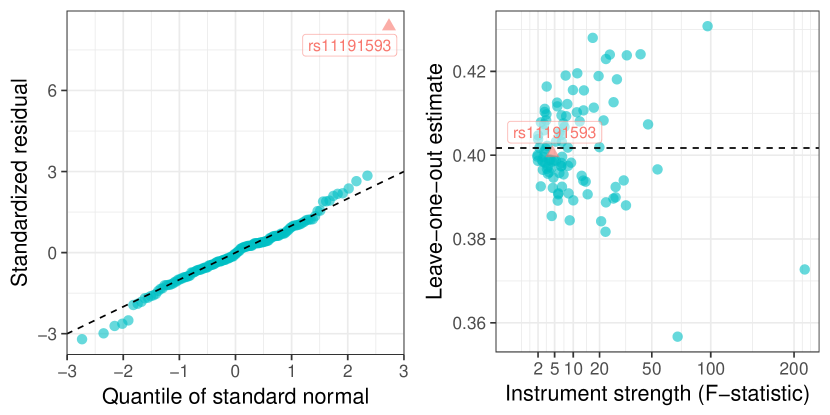
(b) RAPS using the Tukey loss.

Figure 5: Diagnostic plots of the Robust Adjusted Profile Score (RAPS) estimator. Left panels are Q-Q plots of the standardized residuals against standard normal. Right panels are the leave-one-out estimates against instrument strength.

6 Simulation

Throughout the paper all of our theoretical results are asymptotic. We usually require both the sample size $n$ and the number of IVs $p$ to go to infinity (except for Theorem 3.2 where finite $p$ is allowed). We now assess if the asymptotic approximations are reasonably accurate in practical situations, where $p$ may range from tens to hundreds.

6.1 Simulating summary data directly from Assumption 1

To this end, we first created simulated summary-data MR datasets that mimic the BMI-SBP example in Section 1.2. In particular, we considered two scenarios: $p=25$, which corresponds to using the selection threshold $5\times 10^{-8}$ as described in Section 1.2, and $p=160$, which corresponds to using the threshold $1\times 10^{-4}$ as in Sections 3.5, 4.4 and 5.3. The model parameters are chosen as follows: the variances of the measurement error, $\{(\sigma_{Xj}^{2},\sigma_{Yj}^{2})\}_{j\in[p]}$, are the same as those in the BMI-SBP dataset. The true marginal IV-exposure effects, $\{\gamma_{j}\}_{j\in[p]}$, are chosen to be the observed effects in the BMI-SBP dataset, and $\hat{\gamma}_{j}$ is generated according to Assumption 1 by $\hat{\gamma}_{j}\overset{ind.}{\sim}\mathrm{N}(\gamma_{j},\sigma_{Xj}^{2})$. The true marginal IV-outcome effects, $\{\Gamma_{j}\}_{j\in[p]}$, are generated in six different ways with $\beta_{0}=0.4$:

1. $\Gamma_{j}=\gamma_{j}\beta_{0}$;

2. $\Gamma_{j}=\gamma_{j}\beta_{0}+\alpha_{j}$, $\alpha_{j}\overset{i.i.d.}{\sim}\mathrm{N}(0,\tau_{0}^{2})$, where $\tau_{0}=2\cdot(1/p)\sum_{j=1}^{p}\sigma_{Yj}$;

3. $\Gamma_{j}$ is generated according to setup $2$ above, except that $\alpha_{1}$ has mean $5\cdot\tau_{0}$ (the IVs are sorted so that the first IV has the largest $|\gamma_{j}|/\sigma_{Xj}$).

4. $\Gamma_{j}=\gamma_{j}\beta_{0}+\alpha_{j}$, $\alpha_{j}\overset{i.i.d.}{\sim}\tau_{0}\cdot\mathrm{Lap}(1)$, where $\mathrm{Lap}(1)$ is the Laplace (double exponential) distribution with rate $1$.

5. $\Gamma_{j}=\gamma_{j}\beta_{0}+\alpha_{j}$, $\alpha_{j}=|\gamma_{j}|/(p^{-1}\sum_{j=1}^{p}|\gamma_{j}|)\cdot\mathrm{N}(0,\tau_{0}^{2})$.

6. $\Gamma_{j}$ is generated according to setup $2$ above, except that for 10% randomly selected IVs, their direct effects $\alpha_{j}$ have mean $5\cdot\tau_{0}$.

The first three setups correspond to Models 1, 2 and 3, respectively, and the last three setups violate our modeling assumptions and are used to assess the robustness of the procedures. Finally, $\hat{\Gamma}_{j}$ is generated according to Assumption 1 by $\hat{\Gamma}_{j}\overset{ind.}{\sim}\mathrm{N}(\Gamma_{j},\sigma_{Yj}^{2})$.

We applied six methods to the simulated data (10,000 replications in each setting). The first three are existing methods to benchmark our performance: the inverse variance weighting (IVW) estimator [13], MR-Egger regression [7], and the weighted median estimator [8]. The next three methods are proposed in this paper: the profile score (PS) estimator in Section 3, the adjusted profile score (APS) estimator in Section 4, and the robust adjusted profile score (RAPS) estimator in Section 5 with Tukey’s loss function ($k=4.685$).

Table 1: Simulation results for $p=25$. The summary statistics reported are: bias divided by $\beta_{0}$, root-median-square error (RMSE) divided by $\beta_{0}$, length of the confidence interval (CI) divided by $\beta_{0}$, and the coverage rate of the CI (nominal rate is 95%), all in %.

Setup	Method	Bias %	RMSE %	CI Len. %	Cover. %
1	IVW	$\phantom{00}-2.9$	$\phantom{0}12.7$	$\phantom{0}73.8$	$95.4$
	Egger	$\phantom{00}-7.4$	$\phantom{0}24.4$	$142.3$	$95.3$
	W. Median	$\phantom{00}-5.2$	$\phantom{0}17.0$	$105.5$	$96.5$
	PS	$\phantom{00}-0.1$	$\phantom{0}12.7$	$\phantom{0}74.9$	$95.1$
	APS	$\phantom{00}-0.4$	$\phantom{0}12.7$	$\phantom{0}76.8$	$96.0$
	RAPS	$\phantom{00}-0.4$	$\phantom{0}13.0$	$\phantom{0}79.0$	$96.1$
2	IVW	$\phantom{00}-3.0$	$\phantom{0}29.3$	$167.9$	$93.3$
	Egger	$\phantom{00}-8.2$	$\phantom{0}59.7$	$319.2$	$92.1$
	W. Median	$\phantom{0}-12.8$	$\phantom{0}39.9$	$121.4$	$70.6$
	PS	$\phantom{0}\phantom{-}14.7$	$\phantom{0}36.1$	$\phantom{0}71.4$	$49.2$
	APS	$\phantom{00}-0.2$	$\phantom{0}28.8$	$165.4$	$93.4$
	RAPS	$\phantom{00}-0.1$	$\phantom{0}30.1$	$170.2$	$93.1$
3	IVW	$-115.5$	$115.2$	$225.6$	$48.1$
	Egger	$-264.2$	$262.8$	$409.1$	$25.5$
	W. Median	$\phantom{0}-80.7$	$\phantom{0}79.5$	$151.4$	$47.3$
	PS	$-122.3$	$121.3$	$\phantom{0}66.1$	$\phantom{0}6.9$
	APS	$\phantom{0}-86.2$	$\phantom{0}85.6$	$207.0$	$65.0$
	RAPS	$\phantom{0}-11.6$	$\phantom{0}40.6$	$168.7$	$84.3$
4	IVW	$\phantom{00}-5.1$	$\phantom{0}25.1$	$159.5$	$96.0$
	Egger	$\phantom{0}-54.5$	$\phantom{0}58.8$	$300.9$	$90.0$
	W. Median	$\phantom{0}-22.5$	$\phantom{0}26.0$	$113.2$	$83.8$
	PS	$\phantom{0}\phantom{-}13.4$	$\phantom{0}31.2$	$\phantom{0}71.7$	$55.9$
	APS	$\phantom{00}\phantom{-}4.0$	$\phantom{0}25.6$	$158.4$	$96.1$
	RAPS	$\phantom{00}\phantom{-}2.6$	$\phantom{0}20.3$	$117.5$	$93.3$
5	IVW	$\phantom{00}-2.4$	$\phantom{0}48.2$	$169.7$	$76.3$
	Egger	$\phantom{00}-8.2$	$\phantom{0}98.0$	$321.0$	$72.9$
	W. Median	$\phantom{0}-24.4$	$\phantom{0}60.4$	$136.7$	$56.0$
	PS	$\phantom{0}\phantom{-}15.8$	$\phantom{0}57.2$	$\phantom{0}71.6$	$33.0$
	APS	$\phantom{00}\phantom{-}0.9$	$\phantom{0}46.8$	$183.0$	$81.1$
	RAPS	$\phantom{00}\phantom{-}1.5$	$\phantom{0}44.9$	$169.0$	$78.3$
6	IVW	$\phantom{00}-8.1$	$\phantom{0}64.2$	$382.8$	$94.8$
	Egger	$-102.2$	$134.8$	$723.7$	$90.7$
	W. Median	$\phantom{0}-30.8$	$\phantom{0}50.3$	$130.6$	$63.1$
	PS	$\phantom{-}200.2$	$309.6$	$\phantom{0}82.1$	$\phantom{0}4.1$
	APS	$\phantom{0}\phantom{-}13.7$	$\phantom{0}62.1$	$327.1$	$92.8$
	RAPS	$\phantom{0}\phantom{-}12.3$	$\phantom{0}50.3$	$298.2$	$85.4$

Table 2: Simulation results for $p=160$. The summary statistics reported are: bias divided by $\beta_{0}$, root-median-square error (RMSE) divided by $\beta_{0}$, length of the confidence interval (CI) divided by $\beta_{0}$, and the coverage rate of the CI (nominal rate is 95%), all in %.

Setup	Method	Bias %	RMSE %	CI Len. %	Cover. %
1	IVW	$\phantom{000}-11.1$	$\phantom{00}12.2$	$\phantom{00}51.0$	$87.0$
	Egger	$\phantom{000}-10.1$	$\phantom{00}15.2$	$\phantom{00}79.9$	$92.6$
	W. Median	$\phantom{000}-12.6$	$\phantom{00}15.6$	$\phantom{00}84.3$	$93.9$
	PS	$\phantom{0000}\phantom{-}0.1$	$\phantom{000}9.6$	$\phantom{00}57.0$	$95.2$
	APS	$\phantom{0000}-0.4$	$\phantom{000}9.5$	$\phantom{00}58.3$	$95.8$
	RAPS	$\phantom{0000}-0.5$	$\phantom{000}9.8$	$\phantom{00}59.9$	$95.8$
2	IVW	$\phantom{000}-11.6$	$\phantom{00}23.2$	$\phantom{0}122.5$	$92.6$
	Egger	$\phantom{000}-10.8$	$\phantom{00}34.9$	$\phantom{0}191.5$	$93.6$
	W. Median	$\phantom{000}-25.7$	$\phantom{00}34.3$	$\phantom{0}105.5$	$68.9$
	PS	$\phantom{00}\phantom{-}119.2$	$\phantom{0}119.8$	$\phantom{00}51.0$	$\phantom{0}6.2$
	APS	$\phantom{0000}-0.4$	$\phantom{00}23.0$	$\phantom{0}134.8$	$95.1$
	RAPS	$\phantom{0000}-0.4$	$\phantom{00}23.8$	$\phantom{0}138.7$	$95.1$
3	IVW	$\phantom{000}-70.1$	$\phantom{00}69.9$	$\phantom{0}131.3$	$44.7$
	Egger	$\phantom{00}-125.5$	$\phantom{0}125.6$	$\phantom{0}203.8$	$32.3$
	W. Median	$\phantom{000}-65.0$	$\phantom{00}65.0$	$\phantom{0}111.5$	$41.5$
	PS	$\phantom{0000}\phantom{-}4.1$	$\phantom{00}77.9$	$\phantom{00}44.6$	$15.5$
	APS	$\phantom{000}-47.9$	$\phantom{00}48.3$	$\phantom{0}139.3$	$73.2$
	RAPS	$\phantom{0000}-3.9$	$\phantom{00}27.4$	$\phantom{0}137.9$	$90.6$
4	IVW	$\phantom{000}-11.9$	$\phantom{00}20.5$	$\phantom{0}121.5$	$94.7$
	Egger	$\phantom{000}-13.6$	$\phantom{00}31.5$	$\phantom{0}189.5$	$94.7$
	W. Median	$\phantom{000}-24.1$	$\phantom{00}24.8$	$\phantom{00}93.9$	$80.2$
	PS	$\phantom{00}\phantom{-}134.7$	$\phantom{0}114.3$	$\phantom{00}51.4$	$\phantom{0}7.1$
	APS	$\phantom{0000}\phantom{-}4.8$	$\phantom{00}20.8$	$\phantom{0}133.6$	$96.5$
	RAPS	$\phantom{0000}\phantom{-}4.3$	$\phantom{00}16.1$	$\phantom{00}91.3$	$93.6$
5	IVW	$\phantom{000}-11.0$	$\phantom{00}53.9$	$\phantom{0}139.7$	$62.2$
	Egger	$\phantom{0000}-9.8$	$\phantom{00}92.5$	$\phantom{0}217.7$	$56.9$
	W. Median	$\phantom{000}-56.0$	$\phantom{00}63.7$	$\phantom{0}125.2$	$49.3$
	PS	$\phantom{00}-819.8$	$\phantom{0}244.0$	$\phantom{00}57.8$	$\phantom{0}4.7$
	APS	$\phantom{0000}-0.3$	$\phantom{00}55.3$	$\phantom{0}170.7$	$71.6$
	RAPS	$\phantom{0000}\phantom{-}1.5$	$\phantom{00}48.6$	$\phantom{0}120.4$	$59.8$
6	IVW	$\phantom{000}-12.7$	$\phantom{00}47.2$	$\phantom{0}278.8$	$95.0$
	Egger	$\phantom{000}-16.4$	$\phantom{00}74.2$	$\phantom{0}435.3$	$94.9$
	W. Median	$\phantom{000}-34.9$	$\phantom{00}43.6$	$\phantom{0}115.2$	$63.1$
	PS	$\phantom{-}>999.9$	$>999.9$	$>999.9$	$12.8$
	APS	$\phantom{000}\phantom{-}13.6$	$\phantom{00}50.2$	$\phantom{0}291.2$	$95.2$
	RAPS	$\phantom{000}\phantom{-}10.8$	$\phantom{00}42.7$	$\phantom{0}258.4$	$91.2$

The simulation results are reported in Table 1 for $p=25$ and Table 2 for $p=160$. Here is a summary of the results:

1. In setup 1, the PS estimator has the smallest root-median square error (RMSE) and the shortest confidence interval (CI) with the desired coverage rate. The IVW estimator performs very well when $p=25$ but has considerable bias and less than nominal coverage when $p=160$. The APS and RAPS estimators have slightly longer CI than PS. The MR-Egger and weighted median estimators are less accurate than the other methods.

2. In setup 2, the PS estimator, as well as the weighted median, have substantial bias and perform poorly. The APS estimator is overall the best with very small bias and desired coverage, followed very closely by RAPS. The IVW and MR-Egger estimators also perform quite well, though their relative biases are more than 10% when $p=160$.

3. In setup 3, all estimators besides RAPS have very large bias and poor CI coverage. The RMSE of the RAPS estimator is slightly larger than the RMSE in Model 2, and the coverage of RAPS is slightly below the nominal rate.

4. In setup 4, the direct effects $\alpha_{j}$ are distributed as Laplace instead of normal. The RAPS estimator has the smallest bias and RMSE, though the coverage is slightly below the nominal level.

5. In setup 5, the variance of $\alpha_{j}$ is proportional to $|\gamma_{j}|$. In this case APS and RAPS are approximately unbiased but the coverage is significantly lower than 95%.

6. In setup 6, 10% of the IVs have very large but roughly balanced pleiotropy effects $\alpha_{j}$. All estimators are biased in this case. The RAPS estimator has the smallest RMSE but the CI coverage is slightly below 95%. The IVW and APS estimators have slightly larger RMSE and the CI has the desired coverage rate.

Finally, we briefly remark on the bias of IVW and other existing estimators. In 3.3 we have derived that the IVW estimator is biased towards $0$ and the relative bias is approximately $1/\kappa$. The average instrument strength $\kappa$ in the two settings are $\kappa=33.1$ ($p=25$) and $\kappa=9.1$ ($p=160$). The simulation results for setup 1 in Tables 1 and 2 almost exactly match the prediction from our approximation formula (3.10).

Overall, the RAPS estimator is the clear winner in this simulation: when there is no idiosyncratic outlier (setups 1 and 2), it behaves almost as well as the best performer; when there is an idiosyncratic outlier (setup 3), it still has very small bias and close-to-nominal coverage; when our modeling assumptions are not satisfied (setups 4, 5, 6), it still has the smallest bias and RMSE, though the CI may fail to cover $\beta_{0}$ at the nominal rate.

6.2 Simulating from real genotypes

As pointed out by an anonymous reviewer, the marginal GWAS coefficients might not perfectly follow the distributional assumptions in Assumption 1. In fact, in Section 2.2 we already showed that even in linear structural models the marginal coefficients have small but non-zero covariances. As a proof of concept, we perform another simulation study using real genotypes from the 1000 Genomes Project [16].

In total, the 1000 Genomes Project phase 1 dataset contains the genotypes of 1092 individuals. We simulated the exposure $X$ and outcome $Y$ according to the linear structural equation model (2.3) using the entire 10th chromosome as $Z$ (containing $1,882,663$ genetic variants). $100$ random entries of $\bm{\gamma}$ are set to be non-zero and follow the Laplace distribution with rate $1$. The unmeasured confounder $U$ is simulated from the standard normal distribution and the parameters were set to $\eta_{X}=3,\eta_{Y}=5$. The noise variables were simulated from $E_{X}\sim\mathrm{N}(0,3^{2})$ and $E_{Y}\sim\mathrm{N}(0,5^{2})$. The direct effects $\bm{\alpha}$ had $p_{\alpha}$ random non-zero entries that were simulated from the Laplace distribution with rate $r_{\alpha}$. In total we considered five settings:

1. $\beta=0$, $p_{\alpha}=0$;

2. $\beta=0$, $p_{\alpha}=200$, $r_{\alpha}=0.5$;

3. $\beta=1$, $p_{\alpha}=0$;

4. $\beta=1$, $p_{\alpha}=200$, $r_{\alpha}=0.5$;

5. $\beta=1$, $p_{\alpha}=200$, $r_{\alpha}=1.5$;

In this dataset, $368,977$ variants have minor allele frequency greater $5\%$ and are considered as potential instrumental variables. We used $292$, $400$ and $400$ individuals (random partition) as the selection, exposure and outcome data and obtained GWAS summary data by running marginal linear regressions. We simulated $Y$ using one of the five settings described above. After LD clumping ($p$-value $\leq 5\times 10^{-3}$), $121$ independent variants were selected as IVs, and we applied existing and our methods to these $121$ SNPs. To provide a more comprehensive comparison, we also applied two classical IV estimator, two-stage least squares (2SLS) and limited information maximum likelihood (LIML), to the outcome sample of $400$ individuals. For the LIML estimator we computed the standard error using the “many weak IV asymptotics” [25]. Note that 2SLS and LIML cannot be computed using just the GWAS summary data and they assume all the IVs are valid.

We used $5,000$ replications to obtain the same performance metrics in Section 6.1, which are reported in Table 3. Overall, our estimators (in particular, APS and RAPS) are unbiased and maintain the nominal CI coverage rate in all 5 settings. The three existing estimators—IVW, MR-Egger, and weighted median—are heavily biased towards $0$ when $\beta\neq 0$. Also, notice that their RMSE and CI length are (abnormally) smaller than the RMSE and CI length of the “oracle” LIML estimator that uses individual genotypes. The 2SLS estimator is heavily biased due to weak instruments.

Although the simulation results in Table 3 are encouraging, we want to point out that the sample size and simulation parameters we used might be quite different from actual MR studies. The pleiotropy models (parametrized by $p_{\alpha}$ and $r_{\alpha}$) being tested here are also limited. Nonetheless, this simulation shows that using the statistical framework developed in this paper, it is possible to obtain summary-data MR estimators that perform almost as well as the “oracle” LIML estimator that uses individual data.

Table 3: Results for the numerical simulation using real genotypes. The performance metrics reported are: bias (median $\hat{\beta}$ minus $\beta$), root-median-square error (RMSE), median length of the confidence interval (CI), and the coverage rate of the CI (nominal rate is 95%).

Setup	Method	Bias	RMSE	CI Len.	Coverage %
1	IVW	$\phantom{-}0.00$	$0.08$	$0.42$	$93.1$
	Egger	$\phantom{-}0.00$	$0.11$	$0.62$	$95.1$
	W. Median	$\phantom{-}0.00$	$0.12$	$0.74$	$96.8$
	PS	$\phantom{-}0.01$	$0.26$	$1.42$	$92.9$
	APS	$\phantom{-}0.01$	$0.23$	$1.61$	$98.9$
	RAPS	$\phantom{-}0.00$	$0.23$	$1.76$	$98.2$
	2SLS	$-0.46$	$0.46$	$0.41$	$\phantom{0}0.9$
	LIML	$\phantom{-}0.00$	$0.26$	$1.40$	$94.5$
2	IVW	$-0.02$	$0.08$	$0.45$	$94.0$
	Egger	$-0.02$	$0.11$	$0.65$	$95.4$
	W. Median	$-0.04$	$0.12$	$0.78$	$97.2$
	PS	$-0.06$	$0.29$	$1.42$	$89.2$
	APS	$-0.05$	$0.25$	$1.67$	$98.6$
	RAPS	$-0.05$	$0.25$	$1.82$	$97.5$
	2SLS	$-0.47$	$0.47$	$0.43$	$\phantom{0}1.1$
	LIML	$\phantom{-}0.02$	$0.28$	$1.56$	$95.4$
3	IVW	$-0.63$	$0.63$	$0.43$	$\phantom{0}0.1$
	Egger	$-0.45$	$0.45$	$0.61$	$21.1$
	W. Median	$-0.64$	$0.64$	$0.76$	$\phantom{0}8.7$
	PS	$\phantom{-}0.08$	$0.22$	$1.35$	$96.9$
	APS	$\phantom{-}0.02$	$0.22$	$1.78$	$97.6$
	RAPS	$\phantom{-}0.01$	$0.22$	$1.87$	$93.1$
	2SLS	$-0.46$	$0.46$	$0.41$	$\phantom{0}1.2$
	LIML	$-0.01$	$0.26$	$1.41$	$94.8$
4	IVW	$-0.65$	$0.65$	$0.46$	$\phantom{0}0.2$
	Egger	$-0.47$	$0.47$	$0.65$	$22.4$
	W. Median	$-0.61$	$0.61$	$0.79$	$13.6$
	PS	$\phantom{-}0.13$	$0.26$	$1.39$	$95.1$
	APS	$\phantom{-}0.01$	$0.25$	$1.86$	$96.6$
	RAPS	$-0.01$	$0.24$	$1.95$	$92.2$
	2SLS	$-0.46$	$0.46$	$0.43$	$\phantom{0}1.4$
	LIML	$\phantom{-}0.03$	$0.28$	$1.57$	$95.4$
5	IVW	$-0.68$	$0.68$	$0.62$	$\phantom{0}0.9$
	Egger	$-0.50$	$0.50$	$0.90$	$40.4$
	W. Median	$-0.44$	$0.44$	$0.97$	$57.0$
	PS	$\phantom{-}0.41$	$0.49$	$1.72$	$87.3$
	APS	$\phantom{-}0.01$	$0.37$	$2.40$	$96.8$
	RAPS	$-0.04$	$0.33$	$2.48$	$94.8$
	2SLS	$-0.47$	$0.47$	$0.57$	$10.4$
	LIML	$\phantom{-}0.23$	$0.51$	$2.93$	$97.9$

7 Comparison in real data examples

7.1 In the BMI-SBP example

Table 4 briefly summarize the results using different estimators in this and previous papers for the BMI-SBP example introduced in Section 1.2. Since the ground truth is unknown, we do not know which estimate is closer to the truth. Nevertheless, we can still make two observations. First, the point estimates varied considerably between the methods, so the choice of estimator may make a difference in practice. Second, the PS, IVW, and MR-Egger point estimates changed substantially when all $160$ SNPs were used instead of just the $25$ strongest ones, whereas the RAPS estimators and the weighted median were more stable.

Table 4: Comparison of results in the BMI-SBP example.

Method	$p=25$		$p=160$
	$\hat{\beta}$	SE	$\hat{\beta}$	SE
PS	0.367	0.075	0.601	0.054
APS	0.364	0.133	0.301	0.158
RAPS (Huber)	0.354	0.131	0.378	0.121
RAPS (Tukey)	0.361	0.133	0.402	0.106
IVW	0.332	0.140	0.514	0.102
MR-Egger	0.647	0.283	0.472	0.176
Weighted median	0.516	0.125	0.514	0.102

7.2 An illustration of weak IV bias and selection bias

Finally, we consider another real data validation example, which shall be referred to as the BMI-BMI example. In this example, both the “exposure” and the “outcome” are BMI. Although there is no “causal” effect of BMI on itself, Model 1 for GWAS summary data should technically hold with $\beta_{0}=1$. Therefore, this is a rare scenario where we know the truth in real data. Since there are many SNPs that are only weakly associated with BMI, this example also offers a good opportunity to probe the issue of weak instrument bias and the efficiency gain by including many weak IVs. The downside is that this example does not test the methods’ robustness to pleiotropy because the exposure and outcome are the same trait.

We obtained three GWAS datasets for this example:

BMI-GIANT:

full dataset from the GIANT consortium [35] (i.e. combining BMI-FEM and BMI-MAL), used to select SNPs.

BMI-UKBB-1:

half of the UKBB data, used as the “exposure”.

BMI-UKBB-2:

another half of UKBB data, used as the “outcome”.

We applied in total six methods. Four have been previously developed: besides the three estimators considered in Section 6, we also included the weighted mode estimator of Hartwig, Davey Smith and Bowden [26]. We use the implementation in the TwoSampleMR software package [28] for the existing methods. The last two methods were the PS and RAPS estimators developed in this paper (APS performs similarly to PS and RAPS and is omitted).

The results are reported in Table 5. Overall, the PS and RAPS estimators provided very accurate estimate of $\beta_{0}=1$. PS has the smallest standard error because there is no pleiotropy at all in this example. When there is pleiotropy (as expected in most real studies), PS can perform poorly as demonstrated in Section 6. All the existing methods are biased especially when there are many weak IVs.

In Table 6 we illustrate the danger of selection bias. In this example we discard the BMI-GIANT dataset and use BMI-UKBB-1 for both selection and inference (estimating $\gamma_{j}$). The estimators are biased towards $0$ in almost all cases, even if we only use the genome-wide significant $p$-value threshold $10^{-9}$ or $10^{-8}$. This is because the assumption $\hat{\gamma}_{j}\sim\mathrm{N}(\gamma_{j},\sigma_{Xj}^{2})$ is violated. In fact, due to selection bias, the selected $\hat{\gamma}_{j}$ are stochastically larger than their mean $\gamma_{j}$ (if $\gamma_{j}>0$). Compared with other methods, the MR-Egger regression seems to be less affected by the selection bias.

Table 5: Results of the BMI-BMI example. The true $\beta_{0}$ should be $1$. We considered $8$ selection thresholds $p_{\mathrm{sel}}$ from $1\times 10^{-9}$ to $1\times 10^{-2}$. The mean and median of the $F$-statistics $\hat{\gamma}_{j}^{2}/\sigma_{Xj}^{2}$ are reported. In each setting, we report the point estimate and the standard error of all the methods.

$p_{\mathrm{sel}}$	# SNPs	Mean $F$	IVW	W. Median	W. Mode
1e-9	$\phantom{0}48$	$78.6$	0.983 (0.026)	0.945 (0.039)	0.941 (0.042)
1e-8	$\phantom{0}58$	$69.2$	0.983 (0.024)	0.945 (0.039)	0.939 (0.044)
1e-7	$\phantom{0}84$	$55.0$	0.988 (0.024)	0.945 (0.036)	0.933 (0.041)
1e-6	$126$	$44.1$	0.986 (0.022)	0.944 (0.034)	0.931 (0.038)
1e-5	$186$	$34.3$	0.986 (0.019)	0.943 (0.033)	0.928 (0.039)
1e-4	$287$	$26.1$	0.981 (0.017)	0.941 (0.031)	0.929 (0.035)
1e-3	$474$	$18.8$	0.955 (0.015)	0.903 (0.027)	0.917 (0.231)
1e-2	$812$	$12.7$	0.928 (0.014)	0.879 (0.023)	0.739 (7.130)
$p_{\mathrm{sel}}$	# SNPs	Median $F$	Egger	PS	RAPS
1e-9	$\phantom{0}48$	$51.8$	0.926 (0.055)	0.999 (0.023)	0.998 (0.026)
1e-8	$\phantom{0}58$	$42.0$	0.928 (0.050)	0.999 (0.023)	0.998 (0.025)
1e-7	$\phantom{0}84$	$32.1$	0.905 (0.048)	1.012 (0.021)	1.004 (0.025)
1e-6	$126$	$27.4$	0.881 (0.043)	1.017 (0.019)	1.009 (0.023)
1e-5	$186$	$21.0$	0.874 (0.036)	1.020 (0.018)	1.013 (0.020)
1e-4	$287$	$15.8$	0.921 (0.031)	1.023 (0.017)	1.018 (0.018)
1e-3	$474$	$10.8$	0.913 (0.027)	1.010 (0.016)	1.006 (0.016)
1e-2	$812$	$5.6$	0.909 (0.022)	1.010 (0.015)	1.005 (0.015)

Table 6: Illustration of selection bias. The same BMI-UKBB-1 dataset is used for both selecting SNPs and estimating the SNP-exposure effects $\gamma_{j}$. All estimators are biased (true $\beta_{0}=1$) due to not accounting for selection bias.

$p_{\mathrm{sel}}$	# SNPs	Mean $F$	IVW	W. Median	W. Mode
1e-9	$\phantom{0}110$	$68.63$	0.851 (0.02)	0.83 (0.025)	0.896 (0.046)
1e-8	$\phantom{0}168$	$57.00$	0.823 (0.017)	0.8 (0.022)	0.885 (0.053)
1e-7	$\phantom{0}228$	$50.08$	0.799 (0.016)	0.768 (0.019)	0.886 (0.058)
1e-6	$\phantom{0}305$	$43.92$	0.761 (0.015)	0.736 (0.019)	0.865 (0.079)
1e-5	$\phantom{0}443$	$36.98$	0.721 (0.013)	0.667 (0.016)	0.824 (0.12)
1e-4	$\phantom{0}652$	$30.68$	0.678 (0.012)	0.616 (0.015)	0.593 (0.122)
1e-3	$\phantom{0}929$	$25.36$	0.629 (0.011)	0.57 (0.014)	0.576 (0.096)
1e-2	$1289$	$20.70$	0.592 (0.01)	0.528 (0.013)	0.554 (0.093)
$p_{\mathrm{sel}}$	# SNPs	Median $F$	Egger	PS	RAPS
1e-9	$\phantom{0}110$	$49.20$	1.071 (0.051)	0.871 (0.015)	0.862 (0.021)
1e-8	$\phantom{0}168$	$41.12$	1.018 (0.046)	0.848 (0.014)	0.831 (0.018)
1e-7	$\phantom{0}228$	$37.12$	1.016 (0.043)	0.824 (0.012)	0.803 (0.016)
1e-6	$\phantom{0}305$	$33.68$	1.006 (0.041)	0.793 (0.011)	0.763 (0.016)
1e-5	$\phantom{0}443$	$28.74$	0.957 (0.037)	0.762 (0.01)	0.716 (0.015)
1e-4	$\phantom{0}652$	$23.23$	0.89 (0.033)	0.724 (0.009)	0.66 (0.014)
1e-3	$\phantom{0}929$	$19.12$	0.823 (0.03)	0.687 (0.008)	0.594 (0.013)
1e-2	$1289$	$15.26$	0.749 (0.025)	0.657 (0.008)	0.541 (0.012)

8 Discussion

In this paper we have proposed a systematic approach for two-sample summary-data Mendelian randomization based on modifying the profile score function. By considering increasingly more complex models, we arrived at the Robust Adjusted Profile Score (RAPS) estimator which is robust to both systematic and idiosyncratic pleiotropy and performed excellently in all the numerical examples. Thus we recommend to routinely use the RAPS estimator in practice, especially if the exposure and the outcome are both complex traits.

Our theoretical and empirical results advocate for a new design of two-sample MR. Instead of using just a few strong SNPs (those with large $|\hat{\gamma_{j}}|/\sigma_{Xj}$), we find that adding many (potentially hundreds of) weak SNPs usually substantially decreases the variance of the estimator. This is not feasible with existing methods for MR because they usually require the instruments to be strong. An additional advantage of using many weak instruments is that outliers in the sense of Model 3 are more easily detected, so the results are generally more robust to pleiotropy. There is one caveat: selection bias is more significant for weaker instruments, so a sample-splitting design (such as the one in Section 1.2) should be used.

In Models 2 and 3, we have assumed that the pleiotropy effects are completely independent and normally or nearly normally distributed. We view this assumption as an approximate modeling assumption rather than the precise data generating mechanism. It is motivated by the real data (Section 3.5) and seems to fit the data very well (Section 5.3). It is a special instance of the INstrument Strength Independent of Direct Effect (INSIDE) assumption [10] that is common in the summary-data MR literature. Apart from normality, two other implicit but key assumptions we made are:

1. The pleiotropy effects $\alpha_{j}$ are additive rather than multiplicative (the variance of $\alpha_{j}$ is proportional to $\sigma_{Yj}$) [7]. Multiplicative random effects model are easier to fit especially if the measurement error in $\hat{\gamma}_{j}$ is ignored, however it is quite unrealistic because $\alpha_{j}$ is a population quantity and thus is unlikely to be dependent on a sample quantity (for example, $\sigma_{Yj}$ may vary due to missing data). In contrast, the additive model is well motivated by the linear structural model in 2.3.

2. The pleiotropy effects $\alpha_{j}$ have mean $0$. In comparison, the MR-Egger regression [7] assumes $\alpha_{j}$ has an unknown mean $\mu$ and refers to the case $\mu\neq 0$ as “directional pleiotropy”. We have not seen strong evidence of “directional pleiotropy” in real datasets, and, more importantly, assuming $\mu\neq 0$ implies that there is a “special” allele coding so that $\alpha_{j}\sim\mathrm{N}(\mu,\tau^{2})$. It is thus impossible to obtain estimators of $\beta$ that are invariant to allele recoding without completely reformulating the MR-Egger model. For further details see Bowden et al. [11].

There are many technical challenges in the development of this paper. Due to the nature of the many weak IV problem, the asymptotics we considered are quite different from the classical measurement error literature. In Section 3 we showed the profile likelihood is information biased when there are many weak IVs, and in Section 4.1 we showed the profile likelihood is biased when there is overdispersion caused by systematic pleiotropy. This issue is solved by adjusting the profile score, but the proof of the consistency of the APS estimator is nontrivial. Consistency of the the RAPS estimator is even more challenging and still open because the estimating equations may have multiple roots, although we found its practical performance is usually quite benign. A possible solution is to initialize by another robust and consistent estimator (similar to the MM-estimation in robust regression, see Yohai [56]). However, we are not aware of any other provably robust and consistent estimator in our setting, and deriving such estimator is beyond the scope of this paper.

Software and reproducibility

R code for the methods proposed in this paper can be found in the package mr.raps that is publicly available at https://github.com/qingyuanzhao/mr.raps and can be directly called from TwoSampleMR. Numerical examples can be reproduced by running examples in the R package.

Appendix A Linear model for GWAS summary data

In this Appendix we give additional justifications of the linear model (1.1) for GWAS summary data. We will show (1.1) is very likely to hold in very general situations, much beyond the linear structural model considered in Section 2.

A.1 Binary outcome and logistic model

When the outcome $Y$ is binary, the linear structural model (2.2) is no longer appropriate. Instead, we consider the following logistic model of $Y$ (let $H(t)=1/(1+e^{-t})$ be the logistic link function):

$$X=\sum_{j=1}^{p}\gamma_{j}Z_{j}+\eta_{X}U+E_{X},~{}Y\sim\mathrm{Bernoulli}\big{(}H(\beta X+\eta_{Y}U)\big{)}.$$ (A.1)

Next we derive an approximation of the coefficient $\Gamma_{j}$ when we run a logistic regression of $Y$ on $Z_{j}$. By (A.1), we have

$$\mathbb{P}(Y=1|Z_{j}=z_{j})=\mathbb{E}\big{[}H\big{(}\beta\gamma_{j}z_{j}+E^{\prime}\big{)}\big{]},$$

where $E^{\prime}=\beta\sum_{k\neq j}\gamma_{k}Z_{k}+\beta\eta_{X}U+\beta E_{X}+\eta_{Y}U$. If we assume $E^{\prime}\sim\mathrm{N}(\mu,\sigma_{j}^{2})$, then

$$\mathbb{P}(Y=1|Z_{j}=z_{j})=\int_{-\infty}^{\infty}H\big{(}\mu+\beta\gamma_{j}z_{j}+\sigma_{j}e\big{)}\phi(e)\mathop{}\!\mathrm{d}e.$$

Note that $\sigma_{j}^{2}\approx\sigma^{2}=\mathrm{Var}(\beta X+\eta_{Y}U)$ when $\gamma_{j}$ is small.

To proceed further we introduce a well-known probit approximation of logistic function [15]:

$$H(t)\approx\Phi(t/1.7).$$

By using the following Gaussian integral identity,

$$\int_{-\infty}^{\infty}\Phi(a+bx)\phi(x)\mathop{}\!\mathrm{d}x=\Phi\left(\frac{a}{\sqrt{1+b^{2}}}\right),$$

we obtain

$$\begin{split}\mathbb{P}(Y=1|Z_{j}=z_{j})&\approx\int_{-\infty}^{\infty}\Phi\left(\frac{\mu+\beta\gamma_{j}z_{j}+\sigma e}{1.7}\right)\phi(e)\mathop{}\!\mathrm{d}e\\ &=\Phi\left(\frac{\mu+\beta\gamma_{j}z_{j}}{1.7\sqrt{1+(\sigma/1.7)^{2}}}\right)\\ &\approx H\left(\frac{\mu+\beta\gamma_{j}z_{j}}{\sqrt{1+(\sigma/1.7)^{2}}}\right).\end{split}$$

Therefore $\Gamma_{j}\approx\beta\gamma_{j}/\sqrt{1+(\sigma/1.7)^{2}}$. In other words, model (1.1) is approximately correct with $\beta_{0}=\beta/\sqrt{1+(\sigma/1.7)^{2}}$. The attenuation bias is due to the non-collapsibility of odds ratio [greenland1999confounding]. Notice that although we assumed $E^{\prime}$ is normally distributed in our calculation, this approximation is quite accurate for many other distributions [15, Section 4.8.2]. A similar result can be found in vansteelandt2011instrumental who also discussed the general intepretation of causal odds ratios.

A.2 General situation: a local argument

The linear model (1.1) may actually hold in much broader situations than the linear and logistic models considered above. The main reason is that for most SNPs, the influence on a complex trait $X$ is usually minuscule [12, 31, 41, 46]. Let’s consider a continuous exposure $X$ and the quantity $\mathbb{E}[h(Y)|Z_{j}=1]-\mathbb{E}[h(Y)|Z_{j}=0]$ for some function $h$ of interest. Assuming appropriate differentiability and using the shorthand notation $X(z_{1})=g(z_{1},Z_{2},\dotsc,Z_{p},U,E_{X})$, we have,

$$\begin{split}&\mathbb{E}[h(Y)|Z_{1}=1]-\mathbb{E}[h(Y)|Z_{1}=0]\\ =&\mathbb{E}\big{[}h\big{(}f(X(1),U,E_{Y})\big{)}-h\big{(}f(X(0),U,E_{Y})\big{)}\big{]}\\ \approx&\mathbb{E}[h^{\prime}(f^{(1)}(X,U,E_{Y}))\cdot(X(1)-X(0))],\end{split}$$

where $h^{\prime}$ is th derivative of $h$ and $f^{(1)}$ is the partial derivative of $f$ with respect to its first argument. In this approximation we have used the assumption that $X(1)-X(0)$ is small, i.e. the exposure $X$ is not changed by a single instrument $Z_{1}$ by much.

In many epidemiological problems, the causal effect of $X$ on the outcome $Y$ is also very small compared to the variance of $Y$. Therefore, when it is reasonable to assume that the variability of the term $f^{(1)}(X,U,E_{Y})$ is mostly driven by the noise variable $E_{Y}$ which is independent of $X(0)$ and $X(1)$, we have

$$\mathbb{E}[h(Y)|Z_{1}=1]-\mathbb{E}[h(Y)|Z_{1}=0]\approx\mathbb{E}[h^{\prime}(f^{(1)}(X,U,E_{Y}))]\cdot\mathbb{E}[X(1)-X(0)].$$

The left hand side of the above equation may be regarded as a general version of $\Gamma_{1}$ and $\mathrm{E}[X(1)-X(0)]$ a general version of $\gamma_{1}$. Thus we arrive at the approximation $\Gamma_{1}\approx\beta_{0}\gamma_{1}$ for $\beta_{0}=\mathbb{E}[h^{\prime}(f^{(1)}(X,U,E_{Y}))]$. This may be interpreted as the average of “local” causal effect: let $h$ be the identity function and write the potential outcome $Y(x)=f(x,U,E_{Y})$, then

$$\beta_{0}\approx\lim_{\Delta x\to 0}\frac{\mathbb{E}[Y(X+\Delta x)-Y(X)]}{\Delta x},$$

where the expectation is taken jointly over $X$, $U$, and $E_{Y}$.

The above local argument reflects a meta-analysis interpretation of MR [7]: each SNP can be viewed as randomized experiment that changes the exposure $X$ by just a little. Because all the changes are relatively small compared to the variability of $X$ and $Y$, the relationship between $\gamma_{j}$ and $\Gamma_{j}$ is almost linear. This is why we expect the approximate linear relation (1.1) may hold in many problems beyond those discussed in Sections 2.2 and A.1.

Appendix B Proofs

B.1 Proof of Theorem 3.1

Notice that by Assumption 2, $p/(n^{2}\|\bm{\gamma}\|_{2}^{2})\to 0$ implies that $n\to\infty$. Let $e_{j}=\hat{\Gamma}_{j}-\Gamma_{j}$ and $\epsilon_{j}=\hat{\gamma}_{j}-\gamma_{j}$. After some algebra, we have

$$l(\beta)=-\frac{1}{2}\sum_{j=1}^{p}\frac{\gamma_{j}^{2}(\beta_{0}-\beta)^{2}+(e_{j}-\beta\epsilon_{j})^{2}+2\gamma_{j}(\beta_{0}-\beta)(e_{j}-\beta\epsilon_{j})}{\sigma_{Xj}^{2}\beta^{2}+\sigma_{Yj}^{2}}.$$

Notice that $e_{j}-\beta\epsilon_{j}\sim\mathrm{N}(0,\sigma_{Xj}^{2}\beta^{2}+\sigma_{Yj}^{2})$. By Assumption 3, suppose $\sigma_{Xj}^{2}\geq c_{\sigma}/n$ and $\sigma_{Yj}^{2}\geq c_{\sigma}/n$ for all $j\in[p]$. Using the elementary inequality $2/(a+b)\geq\min(1/a,1/b)$ for $a,b>0$, we obtain

$$\begin{split}&-2l(\beta)\\ =&(\beta_{0}-\beta)^{2}\bigg{[}\sum_{j=1}^{p}\frac{\gamma_{j}^{2}}{\sigma_{Xj}^{2}\beta^{2}+\sigma_{Yj}^{2}}\bigg{]}+p+O_{p}\big{(}\sqrt{p}+\sqrt{n}\|\bm{\gamma}\|\cdot|\beta_{0}-\beta|\big{)}\\ \geq&\frac{1}{2}(\beta_{0}-\beta)^{2}\min\bigg{(}\sum_{j=1}^{p}\frac{\gamma_{j}^{2}}{\sigma_{Yj}^{2}},\sum_{j=1}^{p}\frac{\gamma_{j}^{2}}{\sigma_{Xj}^{2}\beta^{2}}\bigg{)}+p+O_{p}\big{(}\sqrt{p}+\sqrt{n}\|\bm{\gamma}\|\cdot|\beta_{0}-\beta|\big{)}\\ \geq&\frac{n\|\bm{\gamma}\|_{2}^{2}}{2c_{\sigma}}\min\Big{(}(\beta_{0}-\beta)^{2},\frac{(\beta_{0}-\beta)^{2}}{\beta^{2}}\Big{)}+p+O_{p}\big{(}\sqrt{p}+\sqrt{n}\|\bm{\gamma}\|\cdot|\beta_{0}-\beta|\big{)}\\ \end{split}$$

Consider the case $\beta_{0}>0$. By taking derivative, it is easy to verify that $f(\beta)=(\beta_{0}-\beta)^{2}/\beta^{2}$ is decreasing in $\beta$ when $0<\beta<\beta_{0}$ and increasing in $\beta$ when $\beta<0$ or $\beta>\beta_{0}$. Since $f(\beta)\to 1$ as $|\beta|\to\infty$, for any $\epsilon>0$ there exists constant $C(\beta_{0},\epsilon)>0$ such that $\inf_{|\beta-\beta_{0}|\geq\epsilon}(\beta_{0}-\beta)^{2}/\beta^{2}\geq C(\beta_{0},\epsilon)$. Similarly, we can show this is also true for $\beta_{0}<0$ and $\beta_{0}=0$. Also, notice that the last term $O_{p}(\sqrt{n}|\beta_{0}-\beta|)$ is negligible compared to the first term when $|\beta-\beta_{0}|\geq\epsilon$. Let $C^{\prime}(\beta_{0},\epsilon)=\min(\epsilon^{2},C(\beta_{0},\epsilon))>0$. We have

$$\inf_{|\beta-\beta_{0}|\geq\epsilon}-2l(\beta)\geq(1+o_{p}(1))C^{\prime}(\beta_{0},\epsilon)\frac{n\|\bm{\gamma}\|_{2}^{2}}{2c_{\sigma}}+p+O_{p}\big{(}\sqrt{p}\big{)}.$$

Finally, by comparing this to $-2l(\beta_{0})=p+O_{p}(\sqrt{p})$, we have

$$\begin{split}&\mathbb{P}\Big{(}l(\beta_{0})>\sup_{|\beta-\beta_{0}|\geq\epsilon}l(\beta)\Big{)}=\mathbb{P}\Big{(}O_{p}(\sqrt{p})\leq(1+o_{p}(1))C^{\prime}(\beta_{0},\epsilon)\frac{n\|\bm{\gamma}\|_{2}^{2}}{2c_{\sigma}}+O_{p}\big{(}\sqrt{p}\big{)}\Big{)}.\end{split}$$

When $p\ll n^{2}\|\bm{\gamma}\|^{4}$, it is easy to see that this probability converges to $1$.

B.2 Proof of Theorem 3.2

By (3.6) and the consistency of $\hat{\beta}$, we have

$$\begin{split}\hat{\beta}-\beta_{0}&=\frac{-\psi(\beta_{0})}{\psi^{\prime}(\beta_{0})+(1/2)\psi^{\prime\prime}(\tilde{\beta})(\hat{\beta}-\beta_{0})}\\ &=\frac{V_{2}}{\sqrt{V_{1}}}\cdot\frac{-\psi(\beta_{0})/\sqrt{V_{1}}}{[\psi^{\prime}(\beta_{0})+o_{p}(\psi^{\prime\prime}(\tilde{\beta}))]/V_{2}}\end{split}$$

The central limit theorem Equation 3.7 is immediately proven using Slutsky’s lemma after showing the following three lemmas:

Lemma B.1.

$(1/\sqrt{V_{1}})\psi(\beta_{0})\overset{d}{\to}\mathrm{N}(0,1)$.

Lemma B.2.

$(-1/V_{2})\psi^{\prime}(\beta_{0})\overset{p}{\to}1$.

Lemma B.3.

For a neighborhood $\mathcal{N}$ of $\beta_{0}$, $\sup_{\beta\in\mathcal{N}}(1/V_{2})\psi^{\prime\prime}(\beta)=O_{p}(1)$.

Next we prove the three lemmas. For the first lemma, let $\psi_{j}(\beta)$ be the $j$-th summand in (3.5), so $\psi(\beta)=\sum_{j=1}^{p}\psi_{j}(\beta)$. It is easy to show that

$$\psi_{j}(\beta_{0})=\frac{(e_{j}-\beta_{0}\epsilon_{j})[\gamma_{j}(\sigma_{Yj}^{2}+\sigma_{Xj}^{2}\beta_{0}^{2})+e_{j}\sigma_{Xj}^{2}\beta_{0}+\epsilon_{j}\sigma_{Yj}^{2}]}{(\sigma_{Yj}^{2}+\sigma_{Xj}^{2}\beta_{0}^{2})^{2}}.$$ (B.1)

The expectation of $\psi_{j}(\beta_{0})$ is

$$\mathbb{E}[\psi_{j}(\beta_{0})]=\frac{\mathbb{E}[e_{j}^{2}\sigma_{Xj}^{2}\beta_{0}-\epsilon_{j}^{2}\sigma_{Yj}^{2}\beta_{0}]}{(\sigma_{Yj}^{2}+\sigma_{Xj}^{2}\beta_{0}^{2})^{2}}=0.$$

This shows that $\mathbb{E}[\psi(\beta_{0})]=0$. The second moment of $\psi_{j}(\beta_{0})$ is given by

$$\mathbb{E}[\psi_{j}(\beta_{0})^{2}]=A_{j}+B_{j},$$

where

$$A_{j}=\mathbb{E}\bigg{[}\frac{(e_{j}-\beta_{0}\epsilon_{j})^{2}\gamma_{j}^{2}(\sigma_{Yj}^{2}+\sigma_{Xj}^{2}\beta_{0}^{2})^{2}}{(\sigma_{Yj}^{2}+\sigma_{Xj}^{2}\beta_{0}^{2})^{4}}\bigg{]}=\frac{\gamma_{j}^{2}}{\sigma_{Yj}^{2}+\sigma_{Xj}^{2}\beta_{0}^{2}},$$

and

$$\begin{split}B_{j}&=\mathbb{E}\bigg{[}\frac{(e_{j}-\beta_{0}\epsilon_{j})^{2}(e_{j}\sigma_{Xj}^{2}\beta_{0}+\epsilon_{j}\sigma_{Yj}^{2})^{2}}{(\sigma_{Yj}^{2}+\sigma_{Xj}^{2}\beta_{0}^{2})^{4}}\bigg{]}\\ &=\mathbb{E}\bigg{[}\frac{e_{j}^{4}\sigma_{Xj}^{4}\beta_{0}^{2}+\epsilon_{j}^{4}\sigma_{Yj}^{4}\beta_{0}^{2}+e_{j}^{2}\epsilon_{j}^{2}(\sigma_{Yj}^{4}-4\beta_{0}\sigma_{Xj}^{2}\beta_{0}\sigma_{Yj}^{2}+\beta_{0}^{2}\sigma_{Xj}^{4}\beta_{0}^{2})}{(\sigma_{Yj}^{2}+\sigma_{Xj}^{2}\beta_{0}^{2})^{4}}\bigg{]}\\ &=\frac{3\sigma_{Yj}^{4}\sigma_{Xj}^{4}\beta_{0}^{2}+3\sigma_{Xj}^{4}\sigma_{Yj}^{4}\beta_{0}^{2}+\sigma_{Yj}^{2}\sigma_{Xj}^{2}(\sigma_{Yj}^{4}-4\beta_{0}\sigma_{Xj}^{2}\beta_{0}\sigma_{Yj}^{2}+\beta_{0}^{2}\sigma_{Xj}^{4}\beta_{0}^{2})}{(\sigma_{Yj}^{2}+\sigma_{Xj}^{2}\beta_{0}^{2})^{4}}\\ &=\frac{\sigma_{Yj}^{2}\sigma_{Xj}^{2}(\sigma_{Yj}^{4}+2\beta_{0}^{2}\sigma_{Xj}^{2}\sigma_{Yj}^{2}+\beta_{0}^{4}\sigma_{Xj}^{4})}{(\sigma_{Yj}^{2}+\sigma_{Xj}^{2}\beta_{0}^{2})^{4}}\\ &=\frac{\sigma_{Xj}^{2}\sigma_{Yj}^{2}}{(\sigma_{Yj}^{2}+\sigma_{Xj}^{2}\beta_{0}^{2})^{2}}.\end{split}$$

In summary,

$$\begin{split}\mathbb{E}[\psi_{j}(\beta_{0})^{2}]&=\frac{\gamma_{j}^{2}\sigma_{Yj}^{2}+\Gamma_{j}^{2}\sigma_{Xj}^{2}+\sigma_{Xj}^{2}\sigma_{Yj}^{2}}{(\sigma_{Yj}^{2}+\sigma_{Xj}^{2}\beta_{0}^{2})^{2}}.\end{split}$$

Notice that by Assumption 3, $\mathbb{E}[\psi_{j}(\beta_{0})^{2}]=\Theta(n\gamma_{j}^{2}+1)$.

To prove Lemma B.1, we consider two scenarios:

Scenario 1: $p\to\infty$. In this case, we hope to use central limit theorem to show

$$\frac{1}{\sqrt{V_{1}}}\psi(\beta_{0})=\frac{1}{\sqrt{V_{1}}}\sum_{j=1}^{p}\psi_{j}(\beta_{0})\to\mathrm{N}(0,1).$$

Next we check Lyapunov’s condition by computing the third moment of $\psi_{j}(\beta_{0})$. Notice that

$$\begin{split}\mathbb{E}[|\psi_{j}(\beta_{0})|^{3}]&=\frac{\mathbb{E}\big{\{}\big{|}(e_{j}-\beta_{0}\epsilon_{j})^{3}[\gamma_{j}(\sigma_{Yj}^{2}+\sigma_{Xj}^{2}\beta_{0}^{2})+e_{j}\sigma_{Xj}^{2}\beta_{0}+\epsilon_{j}\sigma_{Yj}^{2}]^{3}\big{|}\big{\}}}{(\sigma_{Yj}^{2}+\sigma_{Xj}^{2}\beta_{0}^{2})^{6}}\\ &=\frac{\mathbb{E}[|C_{0}+C_{1}\gamma_{j}+C_{2}\gamma_{j}^{2}+C_{3}\gamma_{j}^{3}|]}{(\sigma_{Yj}^{2}+\sigma_{Xj}^{2}\beta_{0}^{2})^{6}}\\ &\leq\frac{\mathbb{E}[|C_{0}|]+\gamma_{j}\mathbb{E}[|C_{1}|]+\gamma_{j}^{2}\mathbb{E}[|C_{2}|]+\gamma_{j}^{3}\mathbb{E}[|C_{3}|]]}{(\sigma_{Yj}^{2}+\sigma_{Xj}^{2}\beta_{0}^{2})^{6}}\end{split}$$

We omit the detailed expressions for $C_{0}$, $C_{1}$, $C_{2}$ and $C_{3}$ but note that there exists constant $C(\beta_{0})>0$ such that $\mathbb{E}[|C_{i}|]\leq C(\beta_{0})(1/n)^{6-i/2}$ for $i=0,1,2,3$. Therefore

$$\sum_{j=1}^{p}\mathbb{E}[|\psi_{j}(\beta_{0})|^{3}]=O(p+\sqrt{n}\|\bm{\gamma}\|_{1}+n\|\bm{\gamma}\|_{2}^{2}+n^{3/2}\|\bm{\gamma}\|_{3}^{3}).$$

By the Cauchy-Schwarz inequality, $\sqrt{n}\|\bm{\gamma}\|_{1}\leq\sqrt{n}\sqrt{p}\|\bm{\gamma}\|_{2}\leq(p+n\|\bm{\gamma}\|_{2}^{2})/2$. Using the assumption $\|\bm{\gamma}\|_{3}/\|\bm{\gamma}\|_{2}\to 0$, it is easy to show the Lyapunov condition

$$\frac{\sum_{j=1}^{p}\mathbb{E}[|\psi_{j}(\beta_{0})|^{3}]}{\big{\{}\sum_{j=1}^{p}\mathbb{E}[\psi_{j}(\beta_{0})^{2}]\big{\}}^{3/2}}=O\bigg{(}\frac{p+n\|\bm{\gamma}\|_{2}^{2}+n^{3/2}\|\bm{\gamma}\|_{3}^{3}}{(p+n\|\bm{\gamma}\|_{2}^{2})^{3/2}}\bigg{)}\to 0.$$

Scenario 2: $p$ is finite. By the assumption in the Theorem statement, $\kappa=n\|\bm{\gamma}\|_{2}^{2}/p\to\infty$. We can rewrite (B.1) to obtain

$$\begin{split}\psi(\beta_{0})&=\sum_{j=1}^{p}\frac{(e_{j}-\beta_{0}\epsilon_{j})\gamma_{j}}{\sigma_{Yj}^{2}+\sigma_{Xj}^{2}\beta_{0}^{2}}+\sum_{j=1}^{p}\frac{(e_{j}-\beta_{0}\epsilon_{j})[e_{j}\sigma_{Xj}^{2}\beta_{0}+\epsilon_{j}\sigma_{Yj}^{2}]}{(\sigma_{Yj}^{2}+\sigma_{Xj}^{2}\beta_{0}^{2})^{2}}.\end{split}$$

The first term on the right hand side is distributed as $\mathrm{N}(0,V_{2})$ and $V_{2}=\Theta(n\|\bm{\gamma}\|_{2}^{2})$. The second term has variance $O(p)$ and is thus ignorable compared to the first term. Therefore, $(1/\sqrt{V_{2}})\psi(\beta_{0})\overset{d}{\to}\mathrm{N}(0,1)$. Since $p/n\to 0$, it is easy to show that $V_{1}/V_{2}\to 1$. By Slutsky’s lemma, $(1/\sqrt{V_{1}})\psi(\beta_{0})\overset{d}{\to}\mathrm{N}(0,1)$.

Now we turn to Lemma B.2. It suffices to prove $\mathrm{E}[\psi^{\prime}(\beta_{0})]=V_{2}$ and $\mathrm{Var}(\psi^{\prime}(\beta_{0})/V_{2})\to 0$. Next we compute the first two moments of $\psi^{\prime}(\beta_{0})$. By differentiating (3.5), we get

$$\psi^{\prime}(\beta_{0})=\sum_{j=1}^{p}\frac{A_{j}+B_{j}}{(\sigma_{Yj}^{2}+\sigma_{Xj}^{2}\beta_{0}^{2})^{4}},$$

where

$$\begin{split}A_{j}&=(\hat{\Gamma}_{j}^{2}\sigma_{Xj}^{2}-\hat{\gamma}_{j}^{2}\sigma_{Yj}^{2}-2\beta_{0}\hat{\gamma}_{j}\hat{\Gamma}_{j}\sigma_{Xj}^{2})(\sigma_{Yj}^{2}+\sigma_{Xj}^{2}\beta_{0}^{2})^{2},\\ B_{j}&=-(\hat{\Gamma}_{j}-\beta_{0}\hat{\gamma}_{j})(\hat{\gamma}_{j}\sigma_{Yj}^{2}+\hat{\Gamma}_{j}\sigma_{Xj}^{2}\beta_{0})\cdot 2(\sigma_{Yj}^{2}+\sigma_{Xj}^{2}\beta_{0}^{2})\cdot 2\sigma_{Xj}^{2}\beta_{0}.\end{split}$$

The expected values of these two terms are

$$\begin{split}\mathbb{E}[A_{j}]&=\big{[}(\Gamma_{j}^{2}+\sigma_{Yj}^{2})\sigma_{Xj}^{2}-(\gamma_{j}^{2}+\sigma_{Xj}^{2})\sigma_{Yj}^{2}-2\beta_{0}\gamma_{j}\Gamma_{j}\sigma_{Xj}^{2}\big{]}(\sigma_{Yj}^{2}+\sigma_{Xj}^{2}\beta_{0}^{2})^{2}\\ &=-(\gamma_{j}^{2}\sigma_{Yj}^{2}+\Gamma_{j}^{2}\sigma_{Xj}^{2})(\sigma_{Yj}^{2}+\sigma_{Xj}^{2}\beta_{0}^{2})^{2},\end{split}$$

$$\begin{split}\mathbb{E}[B_{j}]&=-\big{[}(\Gamma_{j}^{2}+\sigma_{Yj}^{2})\sigma_{Xj}^{2}\beta_{0}-(\gamma_{j}^{2}+\sigma_{Xj}^{2})\sigma_{Yj}^{2}\beta_{0}+\Gamma_{j}\gamma_{j}(\sigma_{Yj}^{2}-\sigma_{Xj}^{2}\beta_{0}^{2})\big{]}\cdot\\ &\quad\cdot 2(\sigma_{Yj}^{2}+\sigma_{Xj}^{2}\beta_{0}^{2})\cdot 2\sigma_{Xj}^{2}\beta_{0}\\ &=-\big{[}(\Gamma_{j}^{2}\sigma_{Xj}^{2}-\gamma_{j}^{2}\sigma_{Yj}^{2})\beta_{0}+\Gamma_{j}\gamma_{j}(\sigma_{Yj}^{2}-\sigma_{Xj}^{2}\beta_{0}^{2})\big{]}\cdot 4(\sigma_{Yj}^{2}+\sigma_{Xj}^{2}\beta_{0}^{2})\sigma_{Xj}^{2}\beta_{0}\\ &=0.\end{split}$$

Therefore $\mathrm{E}[\psi^{\prime}(\beta_{0})]=-V_{2}$.

For the variance of $\psi^{\prime}(\beta_{0})$, consider any $\beta$ in a neighborhood $\mathcal{N}$ of $\beta$. Our argument is based on the key observation that $\psi_{j}(\beta)$ is a homogeneous quadratic polynomial of $(\tilde{\gamma}_{j},\tilde{e}_{j},\tilde{\epsilon}_{j})=(\sqrt{n}\gamma_{j},\sqrt{n}e_{j},\sqrt{n}\epsilon_{j})$:

$$\psi_{j}(\beta)=\frac{((\beta_{0}-\beta)\tilde{\gamma}_{j}+\tilde{e}_{j}-\beta\tilde{\epsilon}_{j})[(n\sigma_{Xj}^{2}\beta\beta_{0}+n\sigma_{Yj}^{2})\tilde{\gamma}_{j}+(n\sigma_{Xj}^{2}\beta)\tilde{e}_{j}+(n\sigma_{Yj}^{2})\tilde{\epsilon}_{j}]}{(n\sigma_{Xj}^{2}\beta^{2}+n\sigma_{Yj}^{2})^{2}}.$$

Therefore its derivative, $\psi^{\prime}_{j}(\beta)$, remains to be a homogeneous quadratic polynomial of $(\tilde{\gamma}_{j},\tilde{e}_{j},\tilde{\epsilon}_{j})$. This observation suggests that $\mathbb{E}[\psi_{j}^{\prime}(\beta_{0})]$ is a quadratic function of $\tilde{\gamma}_{j}$. Notice that the any term in $\psi^{\prime}_{j}(\beta)$ that has odd degree of $\tilde{\gamma}_{j}$ must have expectation equal to $0$, because it must have odd degree in either $\tilde{e}_{j}$ or $\tilde{\epsilon}_{j}$. A simple calculation then yields $\mathbb{E}[\psi_{j}^{\prime}(\beta)]]=\Theta(\tilde{\gamma}_{j}^{2})$, so for $\beta\in\mathcal{N}$,

$$\mathbb{E}[\psi^{\prime}(\beta)]=\Theta(n\|\bm{\gamma}\|_{2}^{2}).$$

Similarly, the variance $\mathrm{Var}[\psi_{j}^{\prime}(\beta)^{2}]$ is also a quadratic polynomial of $\tilde{\gamma}_{j}$ (because the $\tilde{\gamma}_{j}^{2}$ term in $\psi_{j}^{\prime}(\beta)$ is non-random). Thus for $\beta\in\mathcal{N}$,

$$\mathrm{Var}(\psi^{\prime}(\beta))=O(n\|\bm{\gamma}\|_{2}^{2}+p).$$

Using the assumption $p/(n^{2}\|\bm{\gamma}\|^{4})\to 0$, it is then easy to see that

$$\mathrm{Var}(\psi^{\prime}(\beta_{0}))\ll\big{(}\mathrm{E}[\psi^{\prime}(\beta_{0})]\big{)}^{2}.$$

This concludes the proof of Lemma B.2.

The above argument for $\psi^{\prime}(\beta_{0})$ can also be applied to $\psi^{\prime\prime}(\beta)$ for any $\beta$ in a neighborhood $\mathcal{N}$ of $\beta_{0}$, so $\mathrm{Var}(\psi^{\prime\prime}(\beta))=O(n\|\bm{\gamma}\|_{2}^{2}+p)=o(V_{2}^{2})$. Since $\psi(\beta)$ is smooth in $\beta$, this proves the Lemma B.3.

B.3 Proof of Theorem 3.3

By Theorem 3.2, $\hat{\beta}-\beta_{0}=O_{p}(1/\sqrt{n})$. Thus

$$\sigma_{Yj}^{2}+\sigma_{Xj}^{2}\hat{\beta}^{2}=(\sigma_{Yj}^{2}+\sigma_{Xj}^{2}\beta_{0}^{2})(1+o_{p}(1/n)).$$

This implies that

$$\hat{V}_{1}=(1+o_{p}(1))\cdot\sum_{j=1}^{p}\frac{(\hat{\gamma}_{j}^{2}-\sigma_{Xj}^{2})\sigma_{Yj}^{2}+(\hat{\Gamma}_{j}^{2}-\sigma_{Yj}^{2})\sigma_{Xj}^{2}+\sigma_{Xj}^{2}\sigma_{Yj}^{2}}{(\sigma_{Yj}^{2}+\sigma_{Xj}^{2}\beta_{0}^{2})^{2}}.$$

It is easy to show that the summation on the right hand side has mean $V_{1}$. Similar to the proof of Theorem 3.2, the variance of this term is $O(p)$. Note that $V_{1}=\Theta(n\|\bm{\gamma}\|_{2}^{2}+p)=\Theta(p\cdot(1+\kappa))$, using the assumption in Theorem 3.2 that $p\to\infty$ or $\kappa\to\infty$, $\hat{V}_{1}=(1+o_{p}(1))V_{1}$. Similarly, $\hat{V}_{2}=(1+o_{p}(1))V_{2}$. Equation (3.9) follows immediately from Slutsky’s lemma.

B.4 Proof of Theorem 4.1

To prove consistency of $(\hat{\beta},\hat{\tau}_{0}^{2})$, we need to study the asymptotic behavior of the adjusted profile score. Let $\psi_{1j}(\beta,\tau^{2})$ and $\psi_{2j}(\beta,\tau^{2})$ be the $j$-th term in the summation in (4.2) and (4.3), so $\psi_{i}(\beta,\tau^{2})=\sum_{j=1}^{p}\psi_{ij}(\beta,\tau^{2}),~{}i=1,2$. We first consider the expectation of $\psi_{1j}$ and $\psi_{2j}$:

$$\begin{split}&\mathbb{E}[\psi_{1j}(\beta,\tau^{2})]\\ =&\mathbb{E}\bigg{\{}\frac{[(e_{j}-\beta\epsilon_{j})+(\beta_{0}-\beta)\gamma_{j}][\gamma_{j}(\sigma_{Xj}^{2}\beta\beta_{0}+\sigma_{Yj}^{2}+\tau^{2})+\epsilon_{j}(\sigma_{Yj}^{2}+\tau^{2})+e_{j}\sigma_{Xj}^{2}\beta]}{(\sigma_{Xj}^{2}\beta^{2}+\sigma_{Yj}^{2}+\tau^{2})^{2}}\bigg{\}}\\ =&\frac{(\tau^{2}+\sigma_{Yj}^{2}+\sigma_{Xj}^{2}\beta\beta_{0})(\beta_{0}-\beta)\gamma_{j}^{2}+\sigma_{Xj}^{2}\beta(\tau_{0}^{2}-\tau^{2})}{(\tau^{2}+\sigma_{Yj}^{2}+\sigma_{Xj}^{2}\beta^{2})^{2}},\end{split}$$

and

$$\begin{split}\mathbb{E}[\psi_{2j}(\beta,\tau^{2})]&=\mathbb{E}\bigg{\{}\sigma_{Xj}^{2}\frac{[(e_{j}-\beta\epsilon_{j})+(\beta_{0}-\beta)\gamma_{j}]^{2}-(\tau^{2}+\sigma_{Yj}^{2}+\sigma_{Xj}^{2}\beta^{2})}{(\tau^{2}+\sigma_{Yj}^{2}+\sigma_{Xj}^{2}\beta^{2})^{2}}\bigg{\}}\\ &=\frac{\sigma_{Xj}^{2}(\beta_{0}-\beta)^{2}\gamma_{j}^{2}+\sigma_{Xj}^{2}(\tau_{0}^{2}-\tau^{2})}{(\tau^{2}+\sigma_{Yj}^{2}+\sigma_{Xj}^{2}\beta^{2})^{2}}.\end{split}$$ (B.2)

Now consider the following contrast of the two estimating equations:

$$\tilde{\psi}(\beta,\tau^{2})=\psi_{1}(\beta,\tau^{2})-\beta\psi_{2}(\beta,\tau^{2}).$$

It is straightforward to verify that

$$\begin{split}\mathbb{E}[\tilde{\psi}(\beta,\tau^{2})]=&\sum_{j=1}^{p}\frac{(\beta_{0}-\beta)\gamma_{j}^{2}(\tau^{2}+\sigma_{Yj}^{2}+\sigma_{Xj}^{2}\beta\beta_{0}-\beta\sigma_{Xj}^{2}(\beta_{0}-\beta))}{(\tau^{2}+\sigma_{Yj}^{2}+\sigma_{Xj}^{2}\beta^{2})^{2}}\\ =&\sum_{j=1}^{p}\frac{(\beta_{0}-\beta)\gamma_{j}^{2}}{\tau^{2}+\sigma_{Yj}^{2}+\sigma_{Xj}^{2}\beta^{2}}.\end{split}$$

In other words, $\mathbb{E}[\tilde{\psi}(\beta,\tau^{2})]=0$ if and only if $\beta=\beta_{0}$.

Next we bound the variance of $\tilde{\psi}(\beta,\tau^{2})$ over $\mathcal{B}$. Because of Assumptions 3 and 4, $\mathrm{Var}(\epsilon_{j})=\Theta(1/n)$ and $\mathrm{Var}(e_{j})=\Theta(1/n+1/p)$. Using the inequality $\mathrm{Var}(X+Y)\leq 2[\mathrm{Var}(X)+\mathrm{Var}(Y)]$ repeatedly, we have

$$\mathrm{Var(\tilde{\psi}(\beta,\tau^{2}))}=O\big{(}\mathrm{Var}(\psi_{1}(\beta,\tau^{2}))\big{)}+O\big{(}\mathrm{Var}(\psi_{2}(\beta,\tau^{2}))\big{)},$$

and, after some algebra,

$$\begin{split}\mathrm{Var}(\psi_{1}(\beta,\tau^{2}))&=O((n+p)\|\bm{\gamma}\|_{2}^{2}+p)=o(n^{2}),~{}\text{and}\\ \mathrm{Var}(\psi_{2}(\beta,\tau^{2}))&=O((n+p)\|\bm{\gamma}\|_{2}^{2}+p)=o(n^{2}).\end{split}$$

To summarize, we have shown that

$$\tilde{\psi}(\beta,\tau^{2}) =(\beta_{0}-\beta)\cdot\Theta(n)+o_{p}(n),$$ (B.3)

$$\psi_{2}(\beta,\tau^{2}) =(\beta_{0}-\beta)^{2}\Theta(n)+(p\tau_{0}^{2}-p\tau)\Theta(n)+o_{p}(n).$$ (B.4)

Consider a box $\mathcal{B}^{\prime}=[-C_{1},C_{1}]\times[0,C_{2}]$ that contains $\mathcal{B}$. Using (B.3) and (B.4), if $C_{1}$ and $C_{2}/C_{1}$ are sufficiently large, all the following events have probabilities going to $1$:

$$\begin{split}\sup_{|p\tau^{2}|\leq C_{2}}\tilde{\psi}(C_{1},\tau^{2})\leq 0,~{}&\inf_{|p\tau^{2}|\leq C_{2}}\tilde{\psi}(-C_{1},\tau^{2})\geq 0,\\ \sup_{|\beta|\leq C_{1}}\psi_{2}(\beta,C_{2}/p)\leq 0,~{}&\inf_{|\beta|\leq C_{1}}\psi_{2}(\beta,0)\geq 0.\\ \end{split}$$

If all the events are true, by continuity of $\tilde{\psi}$ and $\psi_{2}$ and the Poincaré-Miranda theorem, there exists $(\hat{\beta},p\hat{\tau}^{2})\in\mathcal{B}^{\prime}$ such that

$$\tilde{\psi}(\hat{\beta},\hat{\tau}^{2})=\psi_{2}(\hat{\beta},\hat{\tau}^{2})=0.$$

Using (B.3) and (B.4), it is then straightforward to show $\hat{\beta}\overset{p}{\to}\beta_{0}$ and $(p\hat{\tau}^{2}-p\tau_{0}^{2})\overset{p}{\to}0$. As a consequence, $(\hat{\beta},p\hat{\tau}^{2})\in\mathcal{B}$ with probability going to $1$, thus concluding our proof.

B.5 Proof of Theorem 4.2

We begin with proving $\tilde{\bm{V}}_{1}$ and $\tilde{\bm{V}}_{2}$ are the corresponding moments of $\bm{\psi}(\beta_{0},\tau_{0}^{2})$ and $\nabla\bm{\psi}(\beta_{0},\tau_{0}^{2})$.

Lemma B.4.

$\mathrm{Var}(\bm{\psi}(\beta_{0},\tau_{0}^{2}))=\tilde{\bm{V}}_{1}$, $\mathbb{E}[\nabla\bm{\psi}(\beta_{0},\tau_{0}^{2})]=\tilde{\bm{V}}_{2}$.

Proof of Lemma B.4.

In Section 4.2 we have already shown that $\mathbb{E}[\bm{\psi}(\beta_{0},\tau_{0}^{2})]=\bm{0}$. The variance of $\psi_{1}(\beta_{0},\tau_{0}^{2})$ and the expectation of $(\partial/\partial\beta)\psi_{1}(\beta_{0},\tau_{0}^{2})$ can be obtained from the proof of Theorem 3.2 by replacing $\sigma_{Yj}^{2}$ with $\sigma_{Yj}^{2}+\tau_{0}^{2}$.

Next we compute the other moments. Let $\psi_{1j}(\beta,\tau^{2})$ and $\psi_{2j}(\beta,\tau^{2})$ be the $j$-th summand in (4.2) and (4.3), so $\psi_{i}(\beta,\tau^{2})=\sum_{j=1}^{p}\psi_{ij}(\beta,\tau^{2})$ for $i=1,2$. Because $\hat{\Gamma}_{j}-\beta_{0}\hat{\gamma}_{j}\sim\mathrm{N}(0,\beta_{0}^{2}\sigma_{Xj}^{2}+\Sigma_{Yj}^{2}+\tau_{0}^{2})$, it is easy to see that

$$\mathrm{Var}(\psi_{2j}(\beta_{0},\tau_{0}^{2}))=\frac{2(\sigma_{Xj}^{2})^{2}}{(\sigma_{Xj}^{2}\beta_{0}^{2}+\sigma_{Yj}^{2}+\tau_{0}^{2})^{2}}$$

The covariance of $\psi_{1j}$ and $\psi_{2j}$ is given by

$$\begin{split}&\mathrm{Cov}(\psi_{1j}(\beta_{0},\tau_{0}^{2}),\psi_{2j}(\beta_{0},\tau_{0}^{2}))\\ =&\mathbb{E}\Big{[}\frac{(\hat{\Gamma}_{j}-\beta_{0}\hat{\gamma}_{j})(\hat{\gamma}_{j}(\tau_{0}^{2}+\sigma_{Yj}^{2})+\hat{\Gamma}_{j}\sigma_{Xj}^{2}\beta_{0})\sigma_{Xj}^{2}[(\hat{\Gamma}_{j}-\beta_{0}\hat{\gamma}_{j})^{2}-(\sigma_{Xj}^{2}\beta_{0}^{2}+\sigma_{Yj}^{2}+\tau_{0}^{2})]}{(\sigma_{Xj}^{2}\beta_{0}^{2}+\sigma_{Yj}^{2}+\tau_{0}^{2})^{4}}\Big{]}\\ =&\sigma_{Xj}^{2}\mathbb{E}\Big{[}\frac{(\hat{\Gamma}_{j}-\beta_{0}\hat{\gamma}_{j})^{3}(\hat{\gamma}_{j}(\sigma_{Yj}^{2}+\tau_{0}^{2})+\hat{\Gamma}_{j}\sigma_{Xj}^{2}\beta_{0})}{(\sigma_{Xj}^{2}\beta_{0}^{2}+\sigma_{Yj}^{2}+\tau_{0}^{2})^{4}}\Big{]}\\ =&\sigma_{Xj}^{2}\mathbb{E}\Big{[}\frac{(e_{j}-\beta_{0}\epsilon_{j})^{3}[\gamma_{j}(\sigma_{Xj}^{2}\beta_{0}^{2}+\sigma_{Yj}^{2}+\tau_{0}^{2})+\epsilon_{j}(\sigma_{Yj}^{2}+\tau_{0}^{2})+e_{j}\sigma_{Xj}^{2}\beta_{0}]}{(\sigma_{Xj}^{2}\beta_{0}^{2}+\sigma_{Yj}^{2}+\tau_{0}^{2})^{4}}\Big{]}\\ =&\sigma_{Xj}^{2}\mathbb{E}\Big{[}\frac{(e_{j}-\beta_{0}\epsilon_{j})^{3}[\epsilon_{j}(\sigma_{Yj}^{2}+\tau_{0}^{2})+e_{j}\sigma_{Xj}^{2}\beta_{0}]}{(\sigma_{Xj}^{2}\beta_{0}^{2}+\sigma_{Yj}^{2}+\tau_{0}^{2})^{4}}\Big{]}\\ =&\sigma_{Xj}^{2}\mathbb{E}\Big{[}\frac{e_{j}^{4}\sigma_{Xj}^{2}\beta_{0}+e_{j}^{2}\epsilon_{j}^{2}[-3\beta_{0}(\sigma_{Yj}^{2}+\tau_{0}^{2})+3\beta_{0}^{2}\sigma_{Xj}^{2}\beta_{0}]-\epsilon_{j}^{4}\beta_{0}^{3}(\sigma_{Yj}^{2}+\tau_{0}^{2})}{(\sigma_{Xj}^{2}\beta_{0}^{2}+\sigma_{Yj}^{2}+\tau_{0}^{2})^{4}}\Big{]}\\ =&0.\end{split}$$

Thus $\mathrm{Var}(\bm{\psi}(\beta_{0},\tau_{0}^{2}))=\tilde{\bm{V}}_{1}$. Next we consider the expectation of $\nabla\bm{\psi}(\beta_{0},\tau_{0}^{2})$:

$$\begin{split}&\mathbb{E}\Big{[}\frac{\partial}{\partial\tau^{2}}\psi_{1j}(\beta_{0}^{2},\tau_{0}^{2})\Big{]}\\ =&\mathbb{E}\Big{[}\frac{(\hat{\Gamma}_{j}-\beta_{0}\hat{\gamma}_{j})\hat{\gamma}_{j}(\sigma_{Xj}^{2}\beta_{0}^{2}+\sigma_{Yj}^{2}+\tau_{0}^{2})^{2}}{(\sigma_{Xj}^{2}\beta_{0}^{2}+\sigma_{Yj}^{2}+\tau_{0}^{2})^{4}}\Big{]}-\\ &-\mathbb{E}\Big{[}\frac{(\hat{\Gamma}_{j}-\beta_{0}\hat{\gamma}_{j})(\hat{\gamma}_{j}(\sigma_{Yj}^{2}+\tau_{0}^{2})+\hat{\Gamma}_{j}\sigma_{Xj}^{2}\beta_{0})\cdot 2(\sigma_{Xj}^{2}\beta_{0}^{2}+\sigma_{Yj}^{2}+\tau_{0}^{2})}{(\sigma_{Xj}^{2}\beta_{0}^{2}+\sigma_{Yj}^{2}+\tau_{0}^{2})^{4}}\Big{]}\\ =&\mathbb{E}\Big{[}\frac{(\hat{\Gamma}_{j}-\beta_{0}\hat{\gamma}_{j})[\hat{\gamma}_{j}(\sigma_{Xj}^{2}\beta_{0}^{2}-\sigma_{Yj}^{2}-\tau_{0}^{2})-2\hat{\Gamma}_{j}\sigma_{Xj}^{2}\beta_{0}]}{(\sigma_{Xj}^{2}\beta_{0}^{2}+\sigma_{Yj}^{2}+\tau_{0}^{2})^{3}}\Big{]}\\ =&\mathbb{E}\Big{[}\frac{(e_{j}-\beta_{0}\epsilon_{j})[\epsilon_{j}(\sigma_{Xj}^{2}\beta_{0}^{2}-\sigma_{Yj}^{2}-\tau_{0}^{2})-2e_{j}\sigma_{Xj}^{2}\beta_{0}]}{(\sigma_{Xj}^{2}\beta_{0}^{2}+\sigma_{Yj}^{2}+\tau_{0}^{2})^{3}}\Big{]}\\ =&\frac{-2(\sigma_{Yj}^{2}+\tau_{0}^{2})\sigma_{Xj}^{2}\beta_{0}-\beta_{0}\sigma_{Xj}^{2}(\sigma_{Xj}^{2}\beta_{0}^{2}-\sigma_{Yj}^{2}-\tau_{0}^{2})}{(\sigma_{Xj}^{2}\beta_{0}^{2}+\sigma_{Yj}^{2}+\tau_{0}^{2})^{3}}\\ =&\frac{-\sigma_{Xj}^{2}\beta_{0}}{(\sigma_{Xj}^{2}\beta_{0}^{2}+\sigma_{Yj}^{2}+\tau_{0}^{2})^{2}}.\end{split}$$

Furthermore,

$$\frac{\partial}{\partial\beta}\psi_{2j}(\beta_{0},\tau_{0})=\sigma_{Xj}^{2}\frac{D_{j}-E_{j}}{(\sigma_{Xj}^{2}\beta_{0}^{2}+\sigma_{Yj}^{2}+\tau_{0}^{2})^{4}}$$

where

$$D_{j}=[2(\hat{\Gamma}_{j}-\beta_{0}\hat{\gamma}_{j})(-\hat{\gamma}_{j})-2\sigma_{Xj}^{2}\beta_{0}](\tau_{0}^{2}+\sigma_{Yj}^{2}+\sigma_{Xj}^{2}\beta_{0}^{2})^{2},$$

$$E_{j}=[(\hat{\Gamma}_{j}-\beta_{0}\hat{\gamma}_{j})^{2}-(\tau_{0}^{2}+\sigma_{Yj}^{2}+\sigma_{Xj}^{2}\beta_{0}^{2})]\cdot 2(\tau_{0}^{2}+\sigma_{Yj}^{2}+\sigma_{Xj}^{2}\beta_{0}^{2})\sigma_{Xj}^{2}\cdot 2\beta_{0}.$$

It is not hard to see that both $D_{j}$ and $E_{j}$ have mean $0$. Finally,

$$\begin{split}&\frac{\partial}{\partial\tau_{0}^{2}}\psi_{2j}(\beta_{0},\tau_{0})\\ =&-\frac{\sigma_{Xj}^{2}}{(\sigma_{Xj}^{2}\beta_{0}^{2}+\sigma_{Yj}^{2}+\tau_{0}^{2})^{2}}-\frac{2\sigma_{Xj}^{2}[(\hat{\Gamma}_{j}-\beta_{0}\hat{\gamma}_{j})^{2}-(\sigma_{Xj}^{2}\beta_{0}^{2}+\sigma_{Yj}^{2}+\tau_{0}^{2})]}{(\sigma_{Xj}^{2}\beta_{0}^{2}+\sigma_{Yj}^{2}+\tau_{0}^{2})^{3}}\end{split}$$

It is easy to see that

$$\mathbb{E}\Big{[}\frac{\partial}{\partial\tau^{2}}\psi_{2j}(\beta_{0},\tau_{0})\Big{]}=-\frac{\sigma_{Xj}^{2}}{(\sigma_{Xj}^{2}\beta_{0}^{2}+\sigma_{Yj}^{2}+\tau_{0}^{2})^{2}}.$$

In summary, we have proved that $\mathbb{E}[\nabla\bm{\psi}(\beta_{0},\tau_{0}^{2})]=-\tilde{\bm{V}}_{2}$. ∎

It is useful to write down the order of $\tilde{\bm{V}}_{1}$ and $\tilde{\bm{V}}_{2}$:

$$\begin{split}\tilde{\bm{V}}_{1}&=\begin{pmatrix}\Theta(n)&0\\ 0&\Theta(n)\\ \end{pmatrix},~{}\tilde{\bm{V}}_{2}=\begin{pmatrix}\Theta(n)&\Theta(n^{2})\\ 0&\Theta(n^{2})\\ \end{pmatrix}.\end{split}$$ (B.5)

Similar to the proof of Theorem 3.2, consider the Taylor expansion (let $\bm{\theta}=(\beta,\tau^{2})$)

$$\bm{0}=\bm{\psi}(\hat{\bm{\theta}})=\bm{\psi}(\bm{\theta}_{0})+\nabla\psi(\bm{\theta}_{0})(\hat{\bm{\theta}}-\bm{\theta}_{0})+\frac{1}{2}\begin{pmatrix}(\hat{\bm{\theta}}-\bm{\theta}_{0})^{T}\partial^{2}{\psi}_{1}(\tilde{\bm{\theta}})(\hat{\bm{\theta}}-\bm{\theta}_{0})\\ (\hat{\bm{\theta}}-\bm{\theta}_{0})^{T}\partial^{2}{\psi}_{2}(\tilde{\bm{\theta}})(\hat{\bm{\theta}}-\bm{\theta}_{0}).\end{pmatrix}$$ (B.6)

By the consistency of $(\hat{\beta},p\hat{\tau}^{2})$ and three Lemmas listed after this paragraph, the third term on the right hand side is negligible compared to the second term. The central limit theorem (4.4) can then be proven by the same arguments (normalizing by $\tilde{\bm{V}}_{1}$ and $\tilde{\bm{V}}_{2}$ and using Slutsky’s lemma) as in the beginning of the proof of Theorem 3.2.

Lemma B.5.

$(\tilde{\bm{V}}_{1})^{-1/2}\bm{\psi}(\beta_{0},\tau_{0}^{2})\overset{d}{\to}\mathrm{N}(\bm{0},\bm{I}_{2})$.

Lemma B.6.

$(\tilde{\bm{V}}_{2})^{-1}\nabla\bm{\psi}(\beta_{0},\tau_{0}^{2})\overset{p}{\to}-\bm{I}_{2}$.

Lemma B.7.

Denote $\partial^{2}\psi_{i}(\beta,\tau^{2})$ to be all the second-order partial derivatives of $\psi_{i}(\beta,\tau^{2})$, $i=1,2$. For a neighborhood $\mathcal{N}$ of $(\beta_{0},p\tau_{0}^{2})$ and $l=0,1,2$,

$$\begin{split}\sup_{(\beta,\tau^{2})\in\mathcal{N}}\Big{|}\frac{\partial^{2}}{\partial\beta^{2-l}(\partial\tau^{2})^{l}}\psi_{1}(\beta,\tau^{2})\Big{|}&=O_{p}(n^{l+1}),~{}\text{and}\\ \sup_{(\beta,\tau^{2})\in\mathcal{N}}\Big{|}\frac{\partial^{2}}{\partial\beta^{2-l}(\partial\tau^{2})^{l}}\psi_{2}(\beta,\tau^{2})\Big{|}&=O_{p}(n^{l+1}).\end{split}$$

Next we prove Lemmas B.5, B.6 and B.7. Let $\bm{\psi}_{j}(\beta,\tau^{2})=(\psi_{1j}(\beta,\tau^{2}),\psi_{2j}(\beta,\tau^{2}))$ for $j\in[p]$. Since $\bm{\psi}_{j},j\in[p]$ are mutually independent and $p\to\infty$, it suffices to verify the following Lyapunov condition [bentkus2005lyapunov]

$$\sum_{j=1}^{p}\mathbb{E}\big{[}\|\tilde{\bm{V}}_{1}^{-1/2}\bm{\psi}_{j}(\beta_{0},\tau_{0}^{2})\|^{3}\big{]}\to 0$$

to prove Lemma B.5. Because $\tilde{\bm{V}}_{1}$ is diagonal, it suffices to verify this for each coordinate of $\bm{\psi}_{j}$. Similar to the proof of Lemma B.1, we can show that

$$\sum_{j=1}^{p}\mathbb{E}[|\psi_{1j}(\beta_{0},\tau_{0}^{2})|^{3}]=O(p+\sqrt{n}\|\bm{\gamma}\|_{1}+n\|\bm{\gamma}\|_{2}^{2}+n^{3/2}\|\bm{\gamma}\|_{3}^{3}).$$ (B.7)

Therefore, using $\|\bm{\gamma}\|_{3}/\|\bm{\gamma}\|_{2}\to 0$, we obtain

$$\frac{\sum_{j=1}^{p}\mathbb{E}[|\psi_{1j}(\beta_{0})|^{3}]}{(\tilde{\bm{V}}_{1})_{11}^{3/2}}=O\Big{(}\frac{p+\sqrt{n}\|\bm{\gamma}\|_{1}+n\|\bm{\gamma}\|_{2}^{2}+n^{3/2}\|\bm{\gamma}\|_{3}^{3}}{n^{3/2}}\Big{)}\to 0.$$

For $\psi_{2}$, since the third moment of a $\chi^{2}_{1}$ distribution exists,

$$\mathbb{E}[|\psi_{2j}(\beta_{0},\tau_{0}^{2})|^{3}]=O\Big{(}\frac{\sigma_{Xj}^{6}}{(\sigma_{Xj}^{2}\beta_{0}^{2}+\sigma_{Yj}^{2}+\tau_{0}^{2})^{3}}\Big{)}=O(1).$$

Thus

$$\frac{\sum_{j=1}^{p}\mathbb{E}[|\psi_{2j}(\beta_{0})|^{3}]}{(\tilde{\bm{V}}_{1})_{22}^{3/2}}=O\Big{(}\frac{p}{n^{3/2}}\Big{)}=O(n^{-1/2})\to 0.$$

This completes our proof of Lemma B.5.

For Lemmas B.6 and B.7, it remains to bound the variance of $\nabla\psi$ and $\partial^{2}\psi$. Notice that, similar to the proof of Lemmas B.2 and B.3, $\psi_{1j}(\beta,\tau^{2})$ is a homogeneous quadratic polynomial of $(\tilde{\gamma}_{j},\tilde{e}_{j},\tilde{\epsilon}_{j})=(\gamma_{j}/\sqrt{n},e_{j}/\sqrt{n},\epsilon_{j}/\sqrt{n})$:

$$\begin{split}\psi_{1j}(\beta)=&\frac{\big{[}(\beta_{0}-\beta)\tilde{\gamma}_{j}+\tilde{e}_{j}-\beta\tilde{\epsilon}_{j}\big{]}}{[n\sigma_{Xj}^{2}\beta^{2}+n(\sigma_{Yj}^{2}+\tau^{2})]^{2}}\cdot\\ &\cdot\big{[}(n\sigma_{Xj}^{2}\beta\beta_{0}+n(\sigma_{Yj}^{2}+\tau^{2}))\tilde{\gamma}_{j}+(n\sigma_{Xj}^{2}\beta)\tilde{e}_{j}+(n\sigma_{Yj}^{2})\tilde{\epsilon}_{j}\big{]}.\end{split}$$

Therefore, its derivatives with respect to $\beta$ and $\tau^{2}$ remain to be homogeneous quadratic polynomials. As in the proof of Lemma B.2, this suggests that, for $(\beta,p\tau^{2})\in\mathcal{B}$, (recall that $\|\bm{\gamma}\|_{4}\leq\|\bm{\gamma}\|_{3}\ll\|\bm{\gamma}\|_{2}$)

$$\begin{split}\mathrm{Var}\Big{(}\frac{\partial}{\partial\beta}\psi_{1}(\beta,\tau^{2})\Big{)}&\leq\mathbb{E}\Big{[}\Big{(}\frac{\partial}{\partial\beta}\psi_{1}(\beta,\tau^{2})\Big{)}^{2}\Big{]}\\ &=O\big{(}n^{2}\|\bm{\gamma}\|_{4}^{4}+n\|\bm{\gamma}\|_{2}^{2}+p\big{)}=o((\tilde{\bm{V}}_{2})_{11}^{2}).\end{split}$$ (B.8)

Therefore $(\tilde{\bm{V}}_{2})_{11}^{-1}(\partial/\partial\beta)\psi_{1}(\beta_{0},\tau_{0}^{2})\overset{p}{\to}-1,$ where $(\bm{V})^{-1}_{ij}$ means the reciprocal of the $(i,j)$-th entry of $\bm{V}$. Similarly,

$$\mathrm{Var}\Big{(}(\partial/\partial\tau^{2})\psi_{1}(\beta,\tau^{2})\Big{)}=O\big{(}n[n^{2}\|\bm{\gamma}\|_{4}^{4}+n\|\bm{\gamma}\|_{2}^{2}+p]\big{)}=o((\tilde{\bm{V}}_{2})_{12}^{2}).$$ (B.9)

The extra $n$ comes from differentiating with respect to $\tau^{2}=O(1/p)=O(1/n)$. So $((\tilde{\bm{V}}_{2})_{12})^{-1}(\partial/\partial\tau^{2})\psi_{1}(\beta,\tau^{2})\overset{p}{\to}-1$.

For $\psi_{2}$, we have

$$\psi_{2j}(\beta,\tau^{2})=\frac{\sigma_{Xj}^{2}}{\sigma_{Xj}^{2}\beta_{0}^{2}+\sigma_{Yj}^{2}+\tau_{0}^{2}}\bigg{[}\frac{\big{[}(\beta_{0}-\beta)\tilde{\gamma}_{j}+\tilde{e}_{j}-\beta\tilde{\epsilon}_{j}\big{]}^{2}}{n\sigma_{Xj}^{2}\beta^{2}+n(\sigma_{Yj}^{2}+\tau^{2})}-1\bigg{]}.$$

Using the same argument,

$$\begin{split}\mathrm{Var}\Big{(}(\partial/\partial\beta)\psi_{2}(\beta,\tau^{2})\Big{)}=O\big{(}n^{2}\|\bm{\gamma}\|_{4}^{4}+n\|\bm{\gamma}\|_{2}^{2}+p\big{)}=o((\tilde{\bm{V}}_{2})_{11}),\end{split}$$ (B.10)

$$\begin{split}\mathrm{Var}\Big{(}(\partial/\partial\tau^{2})\psi_{2}(\beta,\tau^{2})\Big{)}&\leq O\big{(}n[n^{2}\|\bm{\gamma}\|_{4}^{4}+n\|\bm{\gamma}\|_{2}^{2}+p]\big{)}=o((\tilde{\bm{V}}_{2})_{22}^{2}).\end{split}$$ (B.11)

Therefore $((\tilde{\bm{V}}_{2})_{22})^{-1}(\partial/\partial\tau^{2})\psi_{2}(\beta,\tau^{2})\overset{p}{\to}-1$. We cannot claim the same conclusion for $(\partial/\partial\tau^{2})\psi_{2}(\beta,\tau^{2})$ because $(\tilde{\bm{V}}_{2})_{21}=0$. Nevertheless, the above results are already enough to verify Lemma B.6, because

$$\begin{split}(\tilde{\bm{V}}_{2})^{-1}\nabla\bm{\psi}(\beta_{0},\tau_{0}^{2})=&\begin{pmatrix}(\tilde{\bm{V}}_{2})_{11}^{-1}&-(\tilde{\bm{V}}_{2})_{11}^{-1}(\tilde{\bm{V}}_{2})_{22}^{-1}(\tilde{\bm{V}}_{2})_{12}\\ 0&(\tilde{\bm{V}}_{2})_{22}^{-1}\end{pmatrix}\begin{pmatrix}\frac{\partial}{\partial\beta}\psi_{1}&\frac{\partial}{\partial\tau^{2}}\psi_{1}\\ \frac{\partial}{\partial\beta}\psi_{2}&\frac{\partial}{\partial\tau^{2}}\psi_{2}\\ \end{pmatrix}\\ =&\begin{pmatrix}(\tilde{\bm{V}}_{2})_{11}^{-1}\frac{\partial}{\partial\beta}\psi_{1}-L\frac{\partial}{\partial\beta}\psi_{2}&(\tilde{\bm{V}}_{2})_{11}^{-1}\frac{\partial}{\partial\tau^{2}}\psi_{1}-L\frac{\partial}{\partial\tau^{2}}\psi_{2}\\ (\tilde{\bm{V}}_{2})_{22}^{-1}\frac{\partial}{\partial\beta}\psi_{2}&(\tilde{\bm{V}}_{2})_{22}^{-1}\frac{\partial}{\partial\tau^{2}}\psi_{2}\\ \end{pmatrix},\end{split}$$

where $L=(\tilde{\bm{V}}_{2})_{11}^{-1}(\tilde{\bm{V}}_{2})_{22}^{-1}(\tilde{\bm{V}}_{2})_{12}=\Theta(n^{-1})$. Using equations B.8, B.9, B.10 and B.11, it is straightforward to verify that the right hand side converges to $\bm{I}_{2}$ in probability.

Finally, Lemma B.7 can be proven similarly to Lemma B.3 using the rate of the variances established above as they also extend to the second-order derivative of $\psi_{2}$.

B.6 Proof of Theorem 5.1

It is easy to show $\mathbb{E}[\psi_{2}^{(\rho)}(\beta_{0},\tau^{2}_{0})]=0$ by using $t_{j}(\beta_{0},\tau_{0}^{2})\sim\mathrm{N}(0,1)$. For $\psi_{1}^{(\rho)}$, since

$$u_{j}(\beta,\tau^{2})=-\frac{\partial}{\partial\beta}t_{j}(\beta,\tau^{2})=\frac{\hat{\Gamma}_{j}\sigma_{Xj}^{2}\beta+\hat{\gamma}_{j}(\sigma_{Yj}^{2}+\tau^{2})}{(\sigma_{Xj}^{2}\beta^{2}+\sigma_{Yj}^{2}+\tau^{2})^{3/2}},$$ (B.12)

it is straightforward to verify that

$$\mathbb{E}\big{[}t_{j}(\beta_{0},\tau_{0}^{2})\cdot u_{j}(\beta_{0},\tau_{0}^{2})\big{]}=\mathbb{E}\bigg{[}\frac{(\hat{\Gamma}_{j}-\beta_{0}\hat{\gamma}_{j})\big{[}\hat{\Gamma}_{j}\sigma_{Xj}^{2}\beta_{0}+\hat{\gamma}_{j}(\sigma_{Yj}^{2}+\tau_{0}^{2})\big{]}}{(\sigma_{Xj}^{2}\beta_{0}^{2}+\sigma_{Yj}^{2}+\tau_{0}^{2})^{2}}\bigg{]}=0.$$

Since $t_{j}(\beta_{0},\tau_{0}^{2})$ and $u_{j}(\beta_{0},\tau_{0}^{2})$ are linear transformations of jointly normal random variables, this implies that $t_{j}(\beta_{0},\tau_{0}^{2})\mathchoice{\mathrel{\hbox to0.0pt{$\displaystyle\perp$\hss}\mkern 2.0mu{\displaystyle\perp}}}{\mathrel{\hbox to0.0pt{$\textstyle\perp$\hss}\mkern 2.0mu{\textstyle\perp}}}{\mathrel{\hbox to0.0pt{$\scriptstyle\perp$\hss}\mkern 2.0mu{\scriptstyle\perp}}}{\mathrel{\hbox to0.0pt{$\scriptscriptstyle\perp$\hss}\mkern 2.0mu{\scriptscriptstyle\perp}}}u_{j}(\beta_{0},\tau_{0}^{2})$. Therefore

$$\mathbb{E}[\psi_{1j}^{(\rho)}(\beta_{0},\tau_{0}^{2})]\propto\mathbb{E}[\rho^{\prime}(t_{j}(\beta_{0},\tau_{0}^{2}))\cdot u_{j}(\beta_{0},\tau_{0}^{2})]=0.$$

By Lemma B.8 below, $\mathrm{E}[\nabla\bm{\psi}^{(\rho)}]=-\tilde{\bm{V}}_{2}^{(\rho)}$ has full rank because $\delta,c_{3}>0$.

B.7 Proof of Theorem 5.2

Similar to the proof of Theorem 4.2, we first show $\tilde{\bm{V}}_{1}^{(\rho)}$ is the variance of $\bm{\psi}^{(\rho)}$ and $\tilde{\bm{V}}_{2}^{(\rho)}$ is the expectation of $-\nabla\bm{\psi}^{(\rho)}$ at the true parameter $(\beta,\tau^{2})=(\beta_{0},\tau_{0}^{2})$.

Lemma B.8.

$\mathrm{Var}\big{(}\bm{\psi}^{(\rho)}(\beta_{0},\tau_{0}^{2})\big{)}=\tilde{\bm{V}}_{1}^{(\rho)}$, $\mathbb{E}\big{[}\nabla\bm{\psi}^{(\rho)}(\beta_{0},\tau_{0}^{2})\big{]}=-\tilde{\bm{V}}_{2}^{(\rho)}$.

Proof of Lemma B.8.

Let $\psi_{1j}^{(\rho)}$ and $\psi_{2j}^{(\rho)}$ be the $j$-th summand in (5.2) and (5.3). We will use the shorthand notation $t_{j0}=t_{j}(\beta_{0},\tau_{0}^{2})$ and $u_{j0}=u_{j}(\beta_{0},\tau_{0}^{2})$.

Because $\rho^{\prime}$ is an odd function and $t_{j0}\sim\mathrm{N}(0,1)$, we have $\mathbb{E}[\rho^{\prime}(t_{j0})]=0$. Using $t_{j0}\mathchoice{\mathrel{\hbox to0.0pt{$\displaystyle\perp$\hss}\mkern 2.0mu{\displaystyle\perp}}}{\mathrel{\hbox to0.0pt{$\textstyle\perp$\hss}\mkern 2.0mu{\textstyle\perp}}}{\mathrel{\hbox to0.0pt{$\scriptstyle\perp$\hss}\mkern 2.0mu{\scriptstyle\perp}}}{\mathrel{\hbox to0.0pt{$\scriptscriptstyle\perp$\hss}\mkern 2.0mu{\scriptscriptstyle\perp}}}u_{j0}$ (see Section B.6), we obtain

$$\begin{split}\mathrm{Var}\big{(}\psi^{(\rho)}_{1j}(\beta_{0},\tau_{0}^{2})\big{)}&=\mathrm{Var}\big{(}\rho^{\prime}(t_{j0}\big{)}u_{j0})=c_{1}\mathbb{E}\big{[}u_{j0}^{2}\big{]}.\end{split}$$

If we let $\rho(r)=r^{2}/2$ be the $l_{2}$-loss (so $c_{1}=1$), we recover the APS so $\mathbb{E}[u_{j0}]=(\tilde{\bm{V}}_{1})_{11}$. Thus $\mathrm{Var}\big{(}\psi^{(\rho)}_{1j}(\beta_{0},\tau_{0}^{2})\big{)}=c_{1}(\tilde{\bm{V}}_{1})_{11}$.

The covariance of $\psi_{1j}^{(\rho)}$ and $\psi_{2j}^{(\rho)}$ is

$$\begin{split}&\mathrm{Cov}\big{(}\psi_{1j}^{(\rho)}(\beta_{0},\tau_{0}^{2}),\psi_{2j}^{(\rho)}(\beta_{0},\tau_{0}^{2})\big{)}\\ \propto&\mathbb{E}\Big{\{}\rho^{\prime}(t_{j0})u_{j0}\cdot\big{[}t_{j0}\rho^{\prime}(t_{j0})-\delta\big{]}\Big{\}}\\ =&\mathbb{E}[u_{j0}]\cdot\mathbb{E}\Big{\{}\rho^{\prime}(t_{j0})\cdot\big{[}t_{j0}\rho^{\prime}(t_{j0})-\delta\big{]}\Big{\}}\\ =&0.\end{split}$$

The last expectation is $0$ because $\rho^{\prime}$ is an odd function.

The variance of $\psi_{2j}^{(\rho)}$ is

$$\begin{split}\mathrm{Var}\big{(}\psi_{2j}^{(\rho)}(\beta_{0},\tau_{0}^{2})\big{)}&=\frac{(\sigma_{Xj}^{2})^{2}}{(\sigma_{Xj}^{2}\beta_{0}^{2}+\sigma_{Yj}^{2}+\tau_{0}^{2})^{2}}\mathrm{Var}\big{(}t_{j0}\rho^{\prime}(t_{j0})\big{)}\\ &=c_{2}(\tilde{\bm{V}}_{1})_{22}.\end{split}$$

Next we turn to the derivatives of $\bm{\psi}^{(\rho)}$. First, by the chain rule,

$$\frac{\partial}{\partial\beta}\psi^{(\rho)}_{1j}(\beta,\tau^{2})=-\rho^{\prime\prime}(t_{j}(\beta,\tau^{2}))u_{j}(\beta,\tau^{2})^{2}+\rho^{\prime}(t_{j}(\beta,\tau^{2}))\frac{\partial}{\partial\beta}u_{j}(\beta,\tau^{2}).$$

The expectation of the first term at $(\beta_{0},\tau_{0}^{2})$ is

$$\mathbb{E}[-\rho^{\prime\prime}(t_{j0})u_{j0}^{2}]=-\mathbb{E}[\rho^{\prime\prime}(t_{j0})]\mathbb{E}[u_{j0}^{2}]=\delta(\tilde{\bm{V}}_{2})_{11},$$

where we have used the identity $\mathbb{E}[\rho^{\prime\prime}(R)]=\mathbb{E}[R\rho^{\prime}(R)]$ for $R\sim\mathrm{N}(0,1)$, which can be proved by integration by parts and the fact that $\phi^{\prime}(x)=-x\phi(x)$. The second term requires more calculations:

$$\begin{split}&\mathbb{E}\Big{[}[\rho^{\prime}(t_{j0})\cdot\Big{(}\frac{\partial}{\partial\beta}u_{j}(\beta,\tau^{2})\Big{)}\Big{|}_{(\beta,\tau^{2})=(\beta_{0},\tau_{0}^{2})}\Big{]}\\ =&\mathbb{E}\bigg{[}\rho^{\prime}(t_{j0})\cdot\frac{\partial}{\partial\beta}\Big{(}\hat{\gamma}_{j}(\tau_{0}^{2}+\sigma_{j2}^{2})+\hat{\Gamma}_{j}\sigma_{j1}^{2}\beta\Big{)}\Big{|}_{\beta=\beta_{0}}\cdot\frac{1}{(\sigma_{Xj}^{2}\beta_{0}^{2}+\sigma_{Yj}^{2}+\tau_{0}^{2})^{3/2}}\bigg{]}\\ &+\mathbb{E}\bigg{[}\rho^{\prime}(t_{j0})\cdot(\hat{\gamma}_{j}(\tau_{0}^{2}+\sigma_{j2}^{2})+\hat{\Gamma}_{j}\sigma_{j1}^{2}\beta_{0})\cdot\frac{\partial}{\partial\beta}\Big{(}\frac{1}{(\sigma_{Xj}^{2}\beta_{0}^{2}+\sigma_{Yj}^{2}+\tau_{0}^{2})^{3/2}}\Big{)}\Big{|}_{\beta=\beta_{0}}\bigg{]}\\ =&\mathbb{E}\bigg{[}\rho^{\prime}(t_{j0})\cdot\frac{\partial}{\partial\beta}\Big{(}\hat{\gamma}_{j}(\tau_{0}^{2}+\sigma_{j2}^{2})+\hat{\Gamma}_{j}\sigma_{j1}^{2}\beta\Big{)}\Big{|}_{\beta=\beta_{0}}\cdot\frac{1}{(\sigma_{Xj}^{2}\beta_{0}^{2}+\sigma_{Yj}^{2}+\tau_{0}^{2})^{3/2}}\bigg{]}\\ =&\mathbb{E}\bigg{[}\rho^{\prime}(t_{j0})\cdot\hat{\Gamma}_{j}\sigma_{j1}^{2}\cdot\frac{1}{(\sigma_{Xj}^{2}\beta_{0}^{2}+\sigma_{Yj}^{2}+\tau_{0}^{2})^{3/2}}\bigg{]}\\ =&\frac{\sigma_{Xj}^{2}}{(\sigma_{Xj}^{2}\beta_{0}^{2}+\sigma_{Yj}^{2}+\tau_{0}^{2})^{3/2}}\mathbb{E}[\rho^{\prime}(t_{j0})(\Gamma_{j}+e_{j})]\\ =&\frac{\sigma_{Xj}^{2}\sqrt{\sigma_{Yj}^{2}+\tau_{0}^{2}}}{(\sigma_{Xj}^{2}\beta_{0}^{2}+\sigma_{Yj}^{2}+\tau_{0}^{2})^{3/2}}\mathbb{E}\bigg{[}\rho^{\prime}(t_{j0})\cdot\frac{e_{j}}{\sqrt{\tau_{0}^{2}+\sigma_{j2}^{2}}}\bigg{]}.\end{split}$$

The second equality above is because $t_{j0}\mathchoice{\mathrel{\hbox to0.0pt{$\displaystyle\perp$\hss}\mkern 2.0mu{\displaystyle\perp}}}{\mathrel{\hbox to0.0pt{$\textstyle\perp$\hss}\mkern 2.0mu{\textstyle\perp}}}{\mathrel{\hbox to0.0pt{$\scriptstyle\perp$\hss}\mkern 2.0mu{\scriptstyle\perp}}}{\mathrel{\hbox to0.0pt{$\scriptscriptstyle\perp$\hss}\mkern 2.0mu{\scriptscriptstyle\perp}}}u_{j0}$ and $\mathbb{E}[\rho^{\prime}(t_{j0})]=0$. Notice that $t_{j0}$ and $e_{j}\big{/}\sqrt{\tau_{0}^{2}+\sigma_{j2}^{2}}$ are marginally distributed as the standard normal and

$$\mathrm{Cov}\bigg{(}t_{j0},\frac{e_{j}}{\sqrt{\sigma_{Yj}^{2}+\tau_{0}^{2}}}\bigg{)}=\Big{(}\frac{\sigma_{Yj}^{2}+\tau_{0}^{2}}{\sigma_{Xj}^{2}\beta_{0}^{2}+\sigma_{Yj}^{2}+\tau_{0}^{2}}\Big{)}^{1/2}.$$

It is not difficult to verify that if $R_{1},R_{2}$ are $\mathrm{N}(0,1)$ marginally and $\mathrm{Cov}(R_{1},R_{2})=\lambda$, then $\mathbb{E}[\rho^{\prime}(R_{1})R_{2}]=\lambda\delta$. Thus

$$\mathbb{E}\Big{[}[\rho^{\prime}(t_{j0})\cdot\frac{\partial}{\partial\beta}u_{j0}\Big{]}=\delta\cdot\frac{\sigma_{Xj}^{2}(\sigma_{Yj}^{2}+\tau_{0}^{2})}{(\sigma_{Xj}^{2}\beta_{0}^{2}+\sigma_{Yj}^{2}+\tau_{0}^{2})^{2}}=\delta[(\tilde{\bm{V}}_{1})_{11}-(\tilde{\bm{V}}_{2})_{11}].$$ (B.13)

To summarize,

$$\begin{split}\mathbb{E}\Big{[}\frac{\partial}{\partial\beta}\psi_{1j}^{(\rho)}(\beta_{0},\tau_{0}^{2})\Big{]}&=-\delta(\tilde{\bm{V}}_{1})_{11}+\delta[(\tilde{\bm{V}}_{1})_{11}-(\tilde{\bm{V}}_{2})_{11}]=-\delta(\tilde{\bm{V}}_{2})_{11}.\end{split}$$

The other first-order derivative of $\psi_{1j}^{(\rho)}$ is

$$\begin{split}\mathbb{E}\bigg{[}\frac{\partial}{\partial\tau^{2}}\psi_{1j}^{(\rho)}(\beta_{0},\tau_{0}^{2})\bigg{]}&=\mathbb{E}\bigg{[}\rho^{\prime\prime}(t_{j0})\Big{(}\frac{\partial}{\partial\tau^{2}}t_{j0}\Big{)}u_{j0}+\rho^{\prime}(t_{j0})\Big{(}\frac{\partial}{\partial\tau^{2}}u_{j0}\Big{)}\bigg{]}.\\ \end{split}$$

Using

$$\frac{\partial}{\partial\tau^{2}}t_{j}(\beta,\tau^{2})=-\frac{t_{j}(\beta,\tau^{2})}{2(\sigma_{Xj}^{2}\beta_{0}^{2}+\sigma_{Yj}^{2}+\tau_{0}^{2})}$$ (B.14)

and the independent of $t_{j0}$, it is straightforward to show the first term has mean $0$. For the second term,

$$\begin{split}\mathbb{E}\bigg{[}\rho^{\prime}(t_{j0})\Big{(}\frac{\partial}{\partial\tau^{2}}u_{j0}\Big{)}\bigg{]}&=\mathbb{E}\bigg{[}\rho^{\prime}(t_{j0})\cdot\hat{\gamma}_{j}\frac{1}{(\sigma_{Xj}^{2}\beta_{0}^{2}+\sigma_{Yj}^{2}+\tau_{0}^{2})^{3/2}}\bigg{]}\\ \end{split}$$

Similar to the derivation of (B.13), one can show that

$$\begin{split}\mathbb{E}\bigg{[}\rho^{\prime}(t_{j0})\Big{(}\frac{\partial}{\partial\tau^{2}}u_{j0}\Big{)}\bigg{]}&=\frac{-\delta\beta_{0}\sigma_{Xj}^{2}}{\sigma_{Xj}^{2}\beta_{0}^{2}+\sigma_{Yj}^{2}+\tau_{0}^{2}}=-\delta\cdot(\tilde{\bm{V}}_{2})_{12}.\end{split}$$

Finally we consider the derivatives of $\psi_{2j}^{(\rho)}$. Using (B.14), we have

$$\begin{split}\mathbb{E}\bigg{[}\frac{\partial}{\partial\tau^{2}}\psi^{(\rho)}_{2j}(\beta_{0},\tau_{0}^{2})\bigg{]}&=\mathbb{E}\bigg{[}\sigma_{Xj}^{2}\frac{-t_{j0}\rho^{\prime}(t_{j0})/2-t_{j0}^{2}\rho^{\prime\prime}(t_{j0})/2-(t_{j0}\rho^{\prime}(t_{j0})-\delta)}{(\sigma_{Xj}^{2}\beta_{0}^{2}+\sigma_{Yj}^{2}+\tau_{0}^{2})^{2}}\bigg{]}\\ &=-\frac{\delta+c_{3}}{2}\cdot\frac{\sigma_{Xj}^{2}}{(\sigma_{Xj}^{2}\beta_{0}^{2}+\sigma_{Yj}^{2}+\tau_{0}^{2})^{2}}\end{split}$$

Hence

$$\mathbb{E}\bigg{[}\frac{\partial}{\partial\tau^{2}}\psi^{(\rho)}_{2}(\beta_{0},\tau_{0}^{2})\bigg{]}=-[(\delta+c_{3})/2](\tilde{\bm{V}}_{2})_{22}.$$

The last partial derivative is $(\partial/\partial\beta)\psi_{2}^{(\rho)}$. Its expectation at $(\beta_{0},\tau_{0}^{2})$ is

$$\begin{split}&\mathbb{E}\Big{[}\frac{\partial}{\partial\beta}\psi^{(\rho)}_{2j}(\beta_{0},\tau_{0}^{2})\Big{]}\\ =&\mathbb{E}\bigg{[}\frac{\frac{\partial}{\partial\beta}\Big{[}t_{j0}\rho^{\prime}(t_{j0})-\delta\Big{]}}{(\sigma_{Xj}^{2}\beta_{0}^{2}+\sigma_{Yj}^{2}+\tau_{0}^{2})^{2}}\bigg{]}\\ &+\mathbb{E}\bigg{[}\frac{\partial}{\partial\beta}\Big{[}\frac{1}{(\sigma_{Xj}^{2}\beta^{2}+\sigma_{Yj}^{2}+\tau_{0}^{2})^{2}}\Big{]}\Big{|}_{\beta=\beta_{0}}\cdot\Big{[}t_{j0}\rho^{\prime}(t_{j0})-\delta\Big{]}\bigg{]}\\ =&\mathbb{E}\bigg{[}\frac{\frac{\partial}{\partial\beta}\Big{[}t_{j0}\rho^{\prime}(t_{j0})-\delta\Big{]}}{(\sigma_{Xj}^{2}\beta_{0}^{2}+\sigma_{Yj}^{2}+\tau_{0}^{2})^{2}}\bigg{]}\\ =&\mathbb{E}\bigg{[}\frac{-u_{j0}\rho^{\prime}(t_{j0})-t_{j0}\rho^{\prime\prime}(t_{j0})u_{j0}}{(\sigma_{Xj}^{2}\beta_{0}^{2}+\sigma_{Yj}^{2}+\tau_{0}^{2})^{2}}\bigg{]}\\ =&0.\end{split}$$

The last equation is due to the independence of $t_{j0}$ and $u_{j0}$ and the fact that $\rho^{\prime}(r)$ and $r\rho^{\prime\prime}(r)$ are odd functions of $r$. ∎

To prove asymptotic normality of the RAPS estimator, we just need to verify Lemmas B.5, B.6 and B.7 with $\bm{\psi}$ replaced by $\bm{\psi}^{(\rho)}$ and $\tilde{\bm{V}}_{1}$, $\tilde{\bm{V}}_{2}$ replaced by $\tilde{\bm{V}}_{1}^{(\rho)}$, $\tilde{\bm{V}}_{2}^{(\rho)}$. This requires verifying the Lyapunov condition for the central limit theorem in Lemma B.5 and bounding the derivatives of $\bm{\psi}^{(\rho)}$ to prove Lemmas B.6 and B.7.

It is useful to notice that the rates of $\tilde{\bm{V}}_{1}$ and $\tilde{\bm{V}}_{2}$ in (B.5) still apply to $\tilde{\bm{V}}_{1}^{(\rho)}$ and $\tilde{\bm{V}}_{2}^{(\rho)}$. First, using the boundedness of $\rho^{\prime}$, we have

$$\sum_{j=1}^{p}\mathbb{E}\big{[}|\psi_{1j}^{(\rho)}(\beta_{0},\tau_{0}^{2})|^{3}\big{]}=\sum_{j=1}^{p}\mathbb{E}[|\rho^{\prime}(t_{j0})|^{3}]\cdot\mathbb{E}[|u_{j0}|^{3}]=O\Big{(}\sum_{j=1}^{p}\mathbb{E}[|u_{j0}|^{3}]\Big{)}.$$

We can rewrite (B.12) as

$$u_{j0}=\frac{(\gamma_{j}\sqrt{n})(\sigma_{Xj}^{2}\beta_{0}+\sigma_{Yj}^{2}+\tau_{0}^{2})+(e_{j}\sqrt{n})(\sigma_{Xj}^{2}\beta_{0})+(\epsilon_{j}\sqrt{n})(\sigma_{Yj}^{2}+\tau_{0}^{2})}{(\sigma_{Xj}^{2}\beta_{0}^{2}+\sigma_{Yj}^{2}+\tau_{0}^{2})^{3/2}\sqrt{n}}.$$

So $u_{j0}$ is a linear combination of $\gamma_{j}\sqrt{n}$, $e_{j}\sqrt{n}$, $\epsilon_{j}\sqrt{n}$. Using the same argument in Section B.5, for any positive integer $k$,

$$\mathbb{E}[|u_{j0}|^{k}]=O\Big{(}\sum_{l=0}^{k}\big{(}\sqrt{n}|\gamma_{j}|+1\big{)}^{l}\Big{)}=O\Big{(}\sum_{l=0}^{k}(\sqrt{n})^{l}|\gamma_{j}|^{l}\Big{)}.$$ (B.15)

From this it is easy to verify equation B.7 still holds for $\psi_{1j}^{(\rho)}(\beta_{0},\tau_{0}^{2})$, $j=1,2,\dotsc$, which implies that

$$\frac{\sum_{j=1}^{p}\mathbb{E}\big{[}\big{|}\psi_{1j}^{(\rho)}(\beta_{0},\tau_{0}^{2})\big{|}^{3}\big{]}}{(\tilde{\bm{V}}_{1}^{(\rho)})_{11}^{3/2}}\to 0.$$

Furthermore,

$$\sum_{j=1}^{p}\mathbb{E}\big{[}|\psi_{2j}^{(\rho)}(\beta_{0},\tau_{0}^{2})|^{3}\big{]}=\sum_{j=1}^{p}\frac{(\sigma_{Xj}^{2})^{3}}{(\sigma_{Xj}^{2}\beta_{0}^{2}+\sigma_{Yj}^{2}+\tau_{0}^{2})^{3}}\cdot c_{5}$$

where $c_{5}=\mathrm{E}[|R\rho^{\prime}(R)-\delta|^{3}]$ for $R\sim\mathrm{N}(0,1)$. Thus

$$\sum_{j=1}^{p}\mathbb{E}\big{[}|\psi_{2j}^{(\rho)}(\beta_{0},\tau_{0}^{2})|^{3}\big{]}=O(p)\ll(\tilde{\bm{V}}_{1}^{(\rho)})_{22}^{3/2}.$$

To summarize, we have verified the Lyapunov condition for $\bm{\psi}_{j}^{(\rho)}$. Consequently, the central limit theorem $(\tilde{\bm{V}}_{1}^{(\rho)})^{-1/2}\bm{\psi}^{(\rho)}(\beta_{0},\tau_{0}^{2})\overset{d}{\to}\mathrm{N}(\bm{0},\bm{I}_{2})$ holds.

Next we restablish the variance bounds, namely equations B.8, B.9, B.10 and B.11, for $\bm{\psi}^{(\rho)}$. Similar to Section B.5, we extend (B.15), the bound on the moments of $u_{j}$, to the derivatives of $u_{j}$: for $(\beta,p\tau^{2})\in\mathcal{B}$,

$$\mathbb{E}\bigg{[}\Big{|}\frac{\partial^{l_{1}+l_{2}}}{\partial\beta^{l_{1}}(\partial\tau^{2})^{l_{2}}}u_{j}(\beta,\tau^{2})\Big{|}^{k}\bigg{]}=O\Big{(}n^{l_{2}}\sum_{l=0}^{k}(\sqrt{n})^{l}|\gamma_{j}|^{l}\Big{)}.$$ (B.16)

Similarly,

$$\mathbb{E}\big{[}\big{|}t_{j}(\beta,\tau^{2})\big{|}^{k}\big{]}=O\Big{(}\sum_{l=0}^{k}(\sqrt{n})^{l}|\gamma_{j}|^{l}\Big{)}.$$ (B.17)

Consider a partial derivative of $\psi^{(\rho)}_{1j}$:

$$\frac{\partial^{l_{1}+l_{2}}}{\partial\beta^{l_{1}}(\partial\tau^{2})^{l_{2}}}\psi^{(\rho)}_{1j}(\beta,\tau^{2})=\frac{\partial^{l_{1}+l_{2}}}{\partial\beta^{l_{1}}(\partial\tau^{2})^{l_{2}}}\rho^{\prime}(t_{j}(\beta,\tau^{2}))u_{j}(\beta,\tau^{2}).$$

By equations B.12 and B.14, It is a polynomial of derivatives (up to $(l_{1}+l_{2}+1)$-th order) of $\rho(t_{j}(\beta,\tau^{2}))$, $t_{j}(\beta,\tau^{2})$, $u_{j}(\beta,\tau^{2})$, and derivatives of $u_{j}(\beta,\tau^{2})$, for which we all have moment bounds. We will use the shorthand notation $t_{j}=t_{j}(\beta,\tau^{2})$ and $u_{j}=u_{j}(\beta,\tau^{2})$ below. In particular,

$$\frac{\partial}{\partial\beta}\psi^{(\rho)}_{1j}(\beta,\tau^{2})=-\rho^{\prime\prime}(t_{j})u_{j}^{2}+\rho^{\prime}(t_{j})\frac{\partial}{\partial\beta}u_{j}.$$

Using the boundedness of $\rho^{\prime}$ and $\rho^{\prime\prime}$ and equation B.16, we have

$$\begin{split}\mathrm{Var}\Big{(}\frac{\partial}{\partial\beta}\psi^{(\rho)}_{1}\Big{)}&\leq\mathrm{E}\Big{[}\Big{(}\frac{\partial}{\partial\beta}\psi^{(\rho)}_{1}\Big{)}^{2}\Big{]}\\ &=O\bigg{(}\sum_{j=1}^{p}u_{j}^{4}+\Big{(}\frac{\partial}{\partial\beta}u_{j}\Big{)}^{2}\bigg{)}\\ &=O\Big{(}\sum_{l=0}^{4}(\sqrt{n})^{l}\|\bm{\gamma}\|_{l}^{l}\Big{)}=o\big{(}(\tilde{\bm{V}}^{(\rho)}_{2})_{11}^{2}\big{)}\end{split}$$

Similarly,

$$\frac{\partial}{\partial\tau^{2}}\psi^{(\rho)}_{1j}=-\rho^{\prime\prime}\big{(}t_{j}\big{)}\frac{t_{j}u_{j}}{2(\sigma_{Xj}^{2}\beta_{0}^{2}+\sigma_{Yj}^{2}+\tau_{0}^{2})}+\rho^{\prime}\big{(}t_{j}\big{)}\frac{\partial}{\partial\tau^{2}}u_{j}.$$

Using the Cauchy-Schwarz inequality, we obtain

$$\begin{split}\mathrm{Var}\Big{(}\frac{\partial}{\partial\tau^{2}}\psi^{(\rho)}_{1}\Big{)}&\leq\mathrm{E}\Big{[}\Big{(}\frac{\partial}{\partial\tau^{2}}\psi^{(\rho)}_{1}\Big{)}^{2}\Big{]}\\ &=O\bigg{(}\mathbb{E}\Big{[}\sum_{j=1}^{p}\frac{t_{j}^{4}+u_{j}^{4}}{(1/n)^{2}}+\Big{(}\frac{\partial}{\partial\tau^{2}}u_{j}\Big{)}^{2}\Big{]}\bigg{)}\\ &=O\Big{(}n^{2}\sum_{l=0}^{4}(\sqrt{n})^{l}\|\bm{\gamma}\|_{l}^{l}+n\sum_{l=0}^{2}(\sqrt{n})^{l}\|\bm{\gamma}\|_{l}^{l}\Big{)}=o\big{(}(\tilde{\bm{V}}^{(\rho)}_{2})_{12}^{2}\big{)}.\end{split}$$

Next we consider the derivatives of $\psi_{2}^{(\rho)}$:

$$\begin{split}\frac{\partial}{\partial\beta}\psi^{(\rho)}_{2j}=&\frac{\sigma_{Xj}^{2}}{\sigma_{Xj}^{2}\beta^{2}+\sigma_{Yj}^{2}+\tau^{2}}\cdot\Big{[}-u_{j}\rho^{\prime}\big{(}t_{j}\big{)}-t_{j}\rho^{\prime\prime}\big{(}t_{j}\big{)}u_{j}\Big{]}-\\ &-\frac{\sigma_{Xj}^{4}\beta}{(\sigma_{Xj}^{2}\beta^{2}+\sigma_{Yj}^{2}+\tau^{2})^{2}}\cdot[t_{j}\rho^{\prime}(t_{j})-\delta],\end{split}$$

thus, again using the Cauchy-Schwarz inequality,

$$\begin{split}\mathrm{E}\Big{[}\Big{(}\frac{\partial}{\partial\beta}\psi^{(\rho)}_{2}\Big{)}^{2}\Big{]}&=O\bigg{(}\mathbb{E}\Big{[}\sum_{j=1}^{p}u_{j}^{2}+(t_{j}^{4}+u_{j}^{4})+t_{j}^{2}\Big{]}\bigg{)}\\ &=O\Big{(}\sum_{l=0}^{4}(\sqrt{n})^{l}\|\bm{\gamma}\|_{l}^{l}\Big{)}=o\big{(}(\tilde{\bm{V}}^{(\rho)}_{2})_{22}\big{)}.\end{split}$$

Finally,

$$\begin{split}\frac{\partial}{\partial\tau^{2}}\psi^{(\rho)}_{2j}=&\frac{\sigma_{Xj}^{2}}{\sigma_{Xj}^{2}\beta^{2}+\sigma_{Yj}^{2}+\tau^{2}}\cdot\Big{[}-\frac{t_{j}}{2(\sigma_{Xj}^{2}\beta^{2}+\sigma_{Yj}^{2}+\tau^{2})}(\rho^{\prime}(t_{j})-t_{j}\rho^{\prime\prime}(t_{j}))\Big{]}-\\ &-\frac{\sigma_{Xj}^{2}}{(\sigma_{Xj}^{2}\beta^{2}+\sigma_{Yj}^{2}+\tau^{2})^{2}}\cdot[t_{j}\rho^{\prime}(t_{j})-\delta].\end{split}$$

Thus

$$\begin{split}\mathrm{E}\Big{[}\Big{(}\frac{\partial}{\partial\tau^{2}}\psi^{(\rho)}_{2}\Big{)}^{2}\Big{]}&=O\bigg{(}\frac{1}{1/n}\mathbb{E}\Big{[}\sum_{j=1}^{p}t_{j}^{2}+t_{j}^{4}\Big{]}\bigg{)}\\ &=O\Big{(}n\sum_{l=0}^{4}(\sqrt{n})^{l}\|\bm{\gamma}\|_{l}^{l}\Big{)}\\ &=o\big{(}(\tilde{\bm{V}}^{(\rho)}_{2})_{22}^{2}\big{)}.\end{split}$$

In summary, we have re-established equations B.8, B.9, B.10 and B.11 for $\bm{\psi}^{(\rho)}$. Therefore Lemma B.6 still holds for $\bm{\psi}^{(\rho)}$ with $\tilde{\bm{V}}_{2}$ replaced by $\tilde{\bm{V}}_{2}^{(\rho)}$.

Finally we prove Lemma B.7 for the RAPS $\bm{\psi}^{(\rho)}$. Notice that, for $(\beta,p\tau^{2})\in\mathcal{B}$, $t_{j}(\beta,\tau^{2})=O_{p}(\sqrt{n}|\gamma_{j}|+1)$ and $u_{j}(\beta,\tau^{2})=O_{p}(\sqrt{n}|\gamma_{j}|+1)$. These rates also hold for the partial derivatives of $t_{j}$ and $u_{j}$ with respect to $\beta$. Therefore, by the boundedness of $\rho^{\prime}$, $\rho^{\prime\prime}$ and $\rho^{\prime\prime\prime}$,

$$\frac{\partial^{2}}{\partial\beta^{2}}\psi_{1j}^{(\rho)}(\beta,\tau^{2})=\rho^{\prime\prime\prime}(t_{j})u_{j}^{3}-3\rho^{\prime\prime}(t_{j})u_{j}\frac{\partial}{\partial\beta}u_{j}+\rho^{\prime}(t_{j})\frac{\partial}{\partial\beta}u_{j}=O_{p}\big{(}(\sqrt{n}|\gamma_{j}|+1)^{3}\big{)}.$$

Hence

$$\frac{\partial^{2}}{\partial\beta^{2}}\psi_{1}^{(\rho)}(\beta,\tau^{2})=\sum_{j=1}^{p}\frac{\partial^{2}}{\partial\beta^{2}}\psi_{1j}^{(\rho)}(\beta,\tau^{2})=O_{p}(p+\sqrt{n}\|\bm{\gamma}\|_{1}+n\|\bm{\gamma}\|_{2}^{2}+n^{3/2}\|\bm{\gamma}\|_{3}^{3}).$$

Using the assumption that $\|\bm{\gamma}\|_{3}^{3}=O(1/\sqrt{p})$, it is easy to show that the right hand side is $O_{p}(n)=O_{p}\big{(}(\tilde{\bm{V}}_{2}^{(\rho)})_{11}\big{)}$. Rates of the other partial derivatives can be proved analogously and we omit further detail.

References

• Clarivate Analytics [2017] {bmisc}[author] \bauthor\bsnmClarivate Analytics (\byear2017). \btitleWeb of Science Topic: Mendelian Randomization. \bnoteData retrieved from http://www.webofknowledge.com. \endbibitem
• Anderson and Rubin [1949] {barticle}[author] \bauthor\bsnmAnderson, \bfnmTheodore W\binitsT. W. and \bauthor\bsnmRubin, \bfnmHerman\binitsH. (\byear1949). \btitleEstimation of the parameters of a single equation in a complete system of stochastic equations. \bjournalAnnals of Mathematical Statistics \bvolume20 \bpages46–63. \endbibitem
• Baiocchi, Cheng and Small [2014] {barticle}[author] \bauthor\bsnmBaiocchi, \bfnmMichael\binitsM., \bauthor\bsnmCheng, \bfnmJing\binitsJ. and \bauthor\bsnmSmall, \bfnmDylan S\binitsD. S. (\byear2014). \btitleInstrumental variable methods for causal inference. \bjournalStatistics in Medicine \bvolume33 \bpages2297–2340. \endbibitem
• Barndorff-Nielsen [1983] {barticle}[author] \bauthor\bsnmBarndorff-Nielsen, \bfnmOle\binitsO. (\byear1983). \btitleOn a formula for the distribution of the maximum likelihood estimator. \bjournalBiometrika \bvolume70 \bpages343–365. \endbibitem
• Bekker [1994] {barticle}[author] \bauthor\bsnmBekker, \bfnmPaul A\binitsP. A. (\byear1994). \btitleAlternative approximations to the distributions of instrumental variable estimators. \bjournalEconometrica \bpages657–681. \endbibitem
• Bound, Jaeger and Baker [1995] {barticle}[author] \bauthor\bsnmBound, \bfnmJohn\binitsJ., \bauthor\bsnmJaeger, \bfnmDavid A\binitsD. A. and \bauthor\bsnmBaker, \bfnmRegina M\binitsR. M. (\byear1995). \btitleProblems with instrumental variables estimation when the correlation between the instruments and the endogenous explanatory variable is weak. \bjournalJournal of American Statistical Association \bvolume90 \bpages443–450. \endbibitem
• Bowden, Davey Smith and Burgess [2015] {barticle}[author] \bauthor\bsnmBowden, \bfnmJack\binitsJ., \bauthor\bsnmDavey Smith, \bfnmGeorge\binitsG. and \bauthor\bsnmBurgess, \bfnmStephen\binitsS. (\byear2015). \btitleMendelian randomization with invalid instruments: effect estimation and bias detection through Egger regression. \bjournalInternational Journal of Epidemiology \bvolume44 \bpages512–525. \endbibitem
• Bowden et al. [2016] {barticle}[author] \bauthor\bsnmBowden, \bfnmJack\binitsJ., \bauthor\bsnmDavey Smith, \bfnmGeorge\binitsG., \bauthor\bsnmHaycock, \bfnmPhilip C\binitsP. C. and \bauthor\bsnmBurgess, \bfnmStephen\binitsS. (\byear2016). \btitleConsistent estimation in Mendelian randomization with some invalid instruments using a weighted median estimator. \bjournalGenetic Epidemiology \bvolume40 \bpages304–314. \endbibitem
• Bowden et al. [2017a] {barticle}[author] \bauthor\bsnmBowden, \bfnmJack\binitsJ., \bauthor\bsnmFabiola Del Greco, \bfnmM\binitsM., \bauthor\bsnmMinelli, \bfnmCosetta\binitsC., \bauthor\bsnmLawlor, \bfnmDebbie\binitsD., \bauthor\bsnmSheehan, \bfnmNuala\binitsN., \bauthor\bsnmThompson, \bfnmJohn\binitsJ. and \bauthor\bsnmSmith, \bfnmGeorge Davey\binitsG. D. (\byear2017a). \btitleImproving the accuracy of two-sample summary data Mendelian randomization: moving beyond the NOME assumption. \bjournalbioRxiv:159442. \endbibitem
• Bowden et al. [2017b] {barticle}[author] \bauthor\bsnmBowden, \bfnmJack\binitsJ., \bauthor\bsnmDel Greco, \bfnmM\binitsM., \bauthor\bsnmMinelli, \bfnmCosetta\binitsC., \bauthor\bsnmDavey Smith, \bfnmGeorge\binitsG., \bauthor\bsnmSheehan, \bfnmNuala\binitsN. and \bauthor\bsnmThompson, \bfnmJohn\binitsJ. (\byear2017b). \btitleA framework for the investigation of pleiotropy in two-sample summary data Mendelian randomization. \bjournalStatistics in Medicine \bvolume36 \bpages1783–1802. \endbibitem
• Bowden et al. [2017c] {barticle}[author] \bauthor\bsnmBowden, \bfnmJack\binitsJ., \bauthor\bsnmSpiller, \bfnmWesley\binitsW., \bauthor\bsnmDel-Greco, \bfnmFabiola\binitsF., \bauthor\bsnmSheehan, \bfnmNuala\binitsN., \bauthor\bsnmThompson, \bfnmJohn\binitsJ., \bauthor\bsnmMinelli, \bfnmCosetta\binitsC. and \bauthor\bsnmSmith, \bfnmGeorge Davey\binitsG. D. (\byear2017c). \btitleImproving the visualisation, interpretation and analysis of two-sample summary data Mendelian randomization via the radial plot and radial regression. \bjournalBioRxiv \bpages200378. \endbibitem
• Boyle, Li and Pritchard [2017] {barticle}[author] \bauthor\bsnmBoyle, \bfnmEvan A\binitsE. A., \bauthor\bsnmLi, \bfnmYang I\binitsY. I. and \bauthor\bsnmPritchard, \bfnmJonathan K\binitsJ. K. (\byear2017). \btitleAn Expanded View of Complex Traits: From Polygenic to Omnigenic. \bjournalCell \bvolume169 \bpages1177–1186. \endbibitem
• Burgess, Butterworth and Thompson [2013] {barticle}[author] \bauthor\bsnmBurgess, \bfnmStephen\binitsS., \bauthor\bsnmButterworth, \bfnmAdam\binitsA. and \bauthor\bsnmThompson, \bfnmSimon G\binitsS. G. (\byear2013). \btitleMendelian randomization analysis with multiple genetic variants using summarized data. \bjournalGenetic Epidemiology \bvolume37 \bpages658–665. \endbibitem
• Burgess et al. [2015] {barticle}[author] \bauthor\bsnmBurgess, \bfnmStephen\binitsS., \bauthor\bsnmScott, \bfnmRobert A\binitsR. A., \bauthor\bsnmTimpson, \bfnmNicholas J\binitsN. J., \bauthor\bsnmSmith, \bfnmGeorge Davey\binitsG. D., \bauthor\bsnmThompson, \bfnmSimon G\binitsS. G. and \bauthor\bsnmConsortium, \bfnmEPIC-InterAct\binitsE.-I. (\byear2015). \btitleUsing published data in Mendelian randomization: a blueprint for efficient identification of causal risk factors. \bjournalEuropean Journal of Epidemiology \bvolume30 \bpages543–552. \endbibitem
• Carroll et al. [2006] {bbook}[author] \bauthor\bsnmCarroll, \bfnmRaymond J\binitsR. J., \bauthor\bsnmRuppert, \bfnmDavid\binitsD., \bauthor\bsnmStefanski, \bfnmLeonard A\binitsL. A. and \bauthor\bsnmCrainiceanu, \bfnmCiprian M\binitsC. M. (\byear2006). \btitleMeasurement Error in Nonlinear Models: A Modern Perspective. \bpublisherCRC press. \endbibitem
• 1000 Genomes Project Consortium [2015] {barticle}[author] \bauthor\bsnm1000 Genomes Project Consortium (\byear2015). \btitleA global reference for human genetic variation. \bjournalNature \bvolume526 \bpages68. \endbibitem
• Cox and Reid [1987] {barticle}[author] \bauthor\bsnmCox, \bfnmDavid Roxbee\binitsD. R. and \bauthor\bsnmReid, \bfnmNancy\binitsN. (\byear1987). \btitleParameter orthogonality and approximate conditional inference. \bjournalJournal of the Royal Statistical Society. Series B (Methodological) \bvolume49 \bpages1–39. \endbibitem
• Davey Smith and Ebrahim [2003] {barticle}[author] \bauthor\bsnmDavey Smith, \bfnmGeorge\binitsG. and \bauthor\bsnmEbrahim, \bfnmShah\binitsS. (\byear2003). \btitle”Mendelian randomization”: can genetic epidemiology contribute to understanding environmental determinants of disease? \bjournalInternational Journal of Epidemiology \bvolume32 \bpages1–22. \endbibitem
• Davey Smith and Hemani [2014] {barticle}[author] \bauthor\bsnmDavey Smith, \bfnmGeorge\binitsG. and \bauthor\bsnmHemani, \bfnmGibran\binitsG. (\byear2014). \btitleMendelian randomization: genetic anchors for causal inference in epidemiological studies. \bjournalHuman Molecular Genetics \bvolume23 \bpagesR89–R98. \endbibitem
• Davey Smith et al. [2007] {barticle}[author] \bauthor\bsnmDavey Smith, \bfnmGeorge\binitsG., \bauthor\bsnmLawlor, \bfnmDebbie A\binitsD. A., \bauthor\bsnmHarbord, \bfnmRoger\binitsR., \bauthor\bsnmTimpson, \bfnmNic\binitsN., \bauthor\bsnmDay, \bfnmIan\binitsI. and \bauthor\bsnmEbrahim, \bfnmShah\binitsS. (\byear2007). \btitleClustered environments and randomized genes: a fundamental distinction between conventional and genetic epidemiology. \bjournalPLoS Medicine \bvolume4 \bpagese352. \endbibitem
• Didelez and Sheehan [2007] {barticle}[author] \bauthor\bsnmDidelez, \bfnmVanessa\binitsV. and \bauthor\bsnmSheehan, \bfnmNuala\binitsN. (\byear2007). \btitleMendelian randomization as an instrumental variable approach to causal inference. \bjournalStatistical Methods in Medical Research \bvolume16 \bpages309–330. \endbibitem
• Fisher [1930] {bbook}[author] \bauthor\bsnmFisher, \bfnmRonald Aylmer\binitsR. A. (\byear1930). \btitleThe Genetical Theory of Natural Selection. \bpublisherOxford University Press. \endbibitem
• Guo et al. [2016] {barticle}[author] \bauthor\bsnmGuo, \bfnmZijian\binitsZ., \bauthor\bsnmKang, \bfnmHyunseung\binitsH., \bauthor\bsnmCai, \bfnmTony T\binitsT. T. and \bauthor\bsnmSmall, \bfnmDylan S\binitsD. S. (\byear2016). \btitleConfidence Intervals for Causal Effects with Invalid Instruments using Two-Stage Hard Thresholding with Voting. \bjournalarXiv:1603.05224. \endbibitem
• Hampel [1974] {barticle}[author] \bauthor\bsnmHampel, \bfnmFrank R\binitsF. R. (\byear1974). \btitleThe influence curve and its role in robust estimation. \bjournalJournal of American Statistical Association \bvolume69 \bpages383–393. \endbibitem
• Hansen, Hausman and Newey [2008] {barticle}[author] \bauthor\bsnmHansen, \bfnmChristian\binitsC., \bauthor\bsnmHausman, \bfnmJerry\binitsJ. and \bauthor\bsnmNewey, \bfnmWhitney\binitsW. (\byear2008). \btitleEstimation with many instrumental variables. \bjournalJournal of Business and Economic Statistics \bvolume26 \bpages398–422. \endbibitem
• Hartwig, Davey Smith and Bowden [2017] {barticle}[author] \bauthor\bsnmHartwig, \bfnmFernando Pires\binitsF. P., \bauthor\bsnmDavey Smith, \bfnmGeorge\binitsG. and \bauthor\bsnmBowden, \bfnmJack\binitsJ. (\byear2017). \btitleRobust inference in two-sample Mendelian randomisation via the zero modal pleiotropy assumption. \bjournalbioRxiv:126102. \endbibitem
• Haycock et al. [2016] {barticle}[author] \bauthor\bsnmHaycock, \bfnmPhilip C\binitsP. C., \bauthor\bsnmBurgess, \bfnmStephen\binitsS., \bauthor\bsnmWade, \bfnmKaitlin H\binitsK. H., \bauthor\bsnmBowden, \bfnmJack\binitsJ., \bauthor\bsnmRelton, \bfnmCaroline\binitsC. and \bauthor\bsnmSmith, \bfnmGeorge Davey\binitsG. D. (\byear2016). \btitleBest (but oft-forgotten) practices: the design, analysis, and interpretation of Mendelian randomization studies. \bjournalThe American journal of clinical nutrition \bvolume103 \bpages965–978. \endbibitem
• Hemani et al. [2016] {barticle}[author] \bauthor\bsnmHemani, \bfnmGibran\binitsG., \bauthor\bsnmZheng, \bfnmJie\binitsJ., \bauthor\bsnmWade, \bfnmKaitlin H\binitsK. H., \bauthor\bsnmLaurin, \bfnmCharles\binitsC., \bauthor\bsnmElsworth, \bfnmBenjamin\binitsB., \bauthor\bsnmBurgess, \bfnmStephen\binitsS., \bauthor\bsnmBowden, \bfnmJack\binitsJ., \bauthor\bsnmLangdon, \bfnmRyan\binitsR., \bauthor\bsnmTan, \bfnmVanessa\binitsV., \bauthor\bsnmYarmolinsky, \bfnmJames\binitsJ., \bauthor\bsnmShihab, \bfnmHashem A.\binitsH. A., \bauthor\bsnmTimpson, \bfnmNicholas\binitsN., \bauthor\bsnmEvans, \bfnmDavid M\binitsD. M., \bauthor\bsnmRelton, \bfnmCaroline\binitsC., \bauthor\bsnmMartin, \bfnmRichard M\binitsR. M., \bauthor\bsnmSmith, \bfnmGeorge Davey\binitsG. D., \bauthor\bsnmGaunt, \bfnmTom R\binitsT. R., \bauthor\bsnmHaycock, \bfnmPhilip C\binitsP. C. and \bauthor\bsnmThe MR-Base Collaboration (\byear2016). \btitleMR-Base: a platform for systematic causal inference across the phenome using billions of genetic associations. \bjournalbioRxiv:078972. \endbibitem
• Hernán and Robins [2006] {barticle}[author] \bauthor\bsnmHernán, \bfnmMiguel A\binitsM. A. and \bauthor\bsnmRobins, \bfnmJames M\binitsJ. M. (\byear2006). \btitleInstruments for causal inference: an epidemiologist’s dream? \bjournalEpidemiology \bvolume17 \bpages360–372. \endbibitem
• Huber [1964] {barticle}[author] \bauthor\bsnmHuber, \bfnmPeter J\binitsP. J. (\byear1964). \btitleRobust estimation of a location parameter. \bjournalAnnals of Mathematical Statistics \bvolume35 \bpages73–101. \endbibitem
• Ioannidis, Trikalinos and Khoury [2006] {barticle}[author] \bauthor\bsnmIoannidis, \bfnmJohn PA\binitsJ. P., \bauthor\bsnmTrikalinos, \bfnmThomas A\binitsT. A. and \bauthor\bsnmKhoury, \bfnmMuin J\binitsM. J. (\byear2006). \btitleImplications of small effect sizes of individual genetic variants on the design and interpretation of genetic association studies of complex diseases. \bjournalAmerican journal of epidemiology \bvolume164 \bpages609–614. \endbibitem
• Kang et al. [2016] {barticle}[author] \bauthor\bsnmKang, \bfnmHyunseung\binitsH., \bauthor\bsnmZhang, \bfnmAnru\binitsA., \bauthor\bsnmCai, \bfnmT Tony\binitsT. T. and \bauthor\bsnmSmall, \bfnmDylan S\binitsD. S. (\byear2016). \btitleInstrumental variables estimation with some invalid instruments and its application to Mendelian randomization. \bjournalJournal of American Statistical Association \bvolume111 \bpages132–144. \endbibitem
• Katan [1986] {barticle}[author] \bauthor\bsnmKatan, \bfnmMartijnB\binitsM. (\byear1986). \btitleApoupoprotein E isoforms, serum cholesterol, and cancer. \bjournalLancet \bvolume327 \bpages507–508. \endbibitem
• Li [2017] {barticle}[author] \bauthor\bsnmLi, \bfnmSai\binitsS. (\byear2017). \btitleMendelian randomization when many instruments are invalid: hierarchical empirical Bayes estimation. \bjournalarXiv:1706.01389. \endbibitem
• Locke et al. [2015] {barticle}[author] \bauthor\bsnmLocke, \bfnmAdam E\binitsA. E., \bauthor\bsnmKahali, \bfnmBratati\binitsB., \bauthor\bsnmBerndt, \bfnmSonja I\binitsS. I., \bauthor\bsnmJustice, \bfnmAnne E\binitsA. E., \bauthor\bsnmPers, \bfnmTune H\binitsT. H., \bauthor\bsnmDay, \bfnmFelix R\binitsF. R., \bauthor\bsnmPowell, \bfnmCorey\binitsC., \bauthor\bsnmVedantam, \bfnmSailaja\binitsS., \bauthor\bsnmBuchkovich, \bfnmMartin L\binitsM. L., \bauthor\bsnmYang, \bfnmJian\binitsJ. \betalet al. (\byear2015). \btitleGenetic studies of body mass index yield new insights for obesity biology. \bjournalNature \bvolume518 \bpages197–206. \endbibitem
• Maronna, Martin and Yohai [2006] {bbook}[author] \bauthor\bsnmMaronna, \bfnmRARD\binitsR., \bauthor\bsnmMartin, \bfnmR Douglas\binitsR. D. and \bauthor\bsnmYohai, \bfnmVictor\binitsV. (\byear2006). \btitleRobust Statistics: Theory and Methods. \bpublisherJohn Wiley & Sons. \endbibitem
• McCullagh and Tibshirani [1990] {barticle}[author] \bauthor\bsnmMcCullagh, \bfnmPeter\binitsP. and \bauthor\bsnmTibshirani, \bfnmRobert\binitsR. (\byear1990). \btitleA simple method for the adjustment of profile likelihoods. \bjournalJournal of the Royal Statistical Society. Series B (Methodological) \bvolume52 \bpages325–344. \endbibitem
• Murphy and Van der Vaart [1996] {barticle}[author] \bauthor\bsnmMurphy, \bfnmS A\binitsS. A. and \bauthor\bparticleVan der \bsnmVaart, \bfnmA W\binitsA. W. (\byear1996). \btitleLikelihood inference in the errors-in-variables model. \bjournalJournal of Multivariate Analysis \bvolume59 \bpages81–108. \endbibitem
• Neyman and Scott [1948] {barticle}[author] \bauthor\bsnmNeyman, \bfnmJerzy\binitsJ. and \bauthor\bsnmScott, \bfnmElizabeth L\binitsE. L. (\byear1948). \btitleConsistent estimates based on partially consistent observations. \bjournalEconometrica \bvolume16 \bpages1–32. \endbibitem
• Pacini and Windmeijer [2016] {barticle}[author] \bauthor\bsnmPacini, \bfnmDavid\binitsD. and \bauthor\bsnmWindmeijer, \bfnmFrank\binitsF. (\byear2016). \btitleRobust inference for the Two-Sample 2SLS estimator. \bjournalEconomics Letters \bvolume146 \bpages50–54. \endbibitem
• Park et al. [2010] {barticle}[author] \bauthor\bsnmPark, \bfnmJu-Hyun\binitsJ.-H., \bauthor\bsnmWacholder, \bfnmSholom\binitsS., \bauthor\bsnmGail, \bfnmMitchell H\binitsM. H., \bauthor\bsnmPeters, \bfnmUlrike\binitsU., \bauthor\bsnmJacobs, \bfnmKevin B\binitsK. B., \bauthor\bsnmChanock, \bfnmStephen J\binitsS. J. and \bauthor\bsnmChatterjee, \bfnmNilanjan\binitsN. (\byear2010). \btitleEstimation of effect size distribution from genome-wide association studies and implications for future discoveries. \bjournalNature Genetics \bvolume42 \bpages570–575. \endbibitem
• Pearl [2009] {bbook}[author] \bauthor\bsnmPearl, \bfnmJudea\binitsJ. (\byear2009). \btitleCausality. \bpublisherCambridge University Press. \endbibitem
• [43] {bmisc}[author] \bauthor\bsnmPurcell, \bfnmShaun\binitsS. \btitlePLINK (software V1.07). \bhowpublishedhttp://pngu.mgh.harvard.edu/purcell/plink/. \endbibitem
• Purcell et al. [2007] {barticle}[author] \bauthor\bsnmPurcell, \bfnmShaun\binitsS., \bauthor\bsnmNeale, \bfnmBenjamin\binitsB., \bauthor\bsnmTodd-Brown, \bfnmKathe\binitsK., \bauthor\bsnmThomas, \bfnmLori\binitsL., \bauthor\bsnmFerreira, \bfnmManuel AR\binitsM. A., \bauthor\bsnmBender, \bfnmDavid\binitsD., \bauthor\bsnmMaller, \bfnmJulian\binitsJ., \bauthor\bsnmSklar, \bfnmPamela\binitsP., \bauthor\bsnmDe Bakker, \bfnmPaul IW\binitsP. I., \bauthor\bsnmDaly, \bfnmMark J\binitsM. J. and \bauthor\bsnmSham, \bfnmPak C\binitsP. C. (\byear2007). \btitlePLINK: a tool set for whole-genome association and population-based linkage analyses. \bjournalAmerican Journal of Human Genetics \bvolume81 \bpages559–575. \endbibitem
• Rothenberg [1971] {barticle}[author] \bauthor\bsnmRothenberg, \bfnmThomas J\binitsT. J. (\byear1971). \btitleIdentification in parametric models. \bjournalEconometrica \bvolume39 \bpages577–591. \endbibitem
• Shi, Kichaev and Pasaniuc [2016] {barticle}[author] \bauthor\bsnmShi, \bfnmHuwenbo\binitsH., \bauthor\bsnmKichaev, \bfnmGleb\binitsG. and \bauthor\bsnmPasaniuc, \bfnmBogdan\binitsB. (\byear2016). \btitleContrasting the genetic architecture of 30 complex traits from summary association data. \bjournalThe American Journal of Human Genetics \bvolume99 \bpages139–153. \endbibitem
• Solovieff et al. [2013] {barticle}[author] \bauthor\bsnmSolovieff, \bfnmNadia\binitsN., \bauthor\bsnmCotsapas, \bfnmChris\binitsC., \bauthor\bsnmLee, \bfnmPhil H\binitsP. H., \bauthor\bsnmPurcell, \bfnmShaun M\binitsS. M. and \bauthor\bsnmSmoller, \bfnmJordan W\binitsJ. W. (\byear2013). \btitlePleiotropy in complex traits: challenges and strategies. \bjournalNature Reviews Genetics \bvolume14 \bpages483–495. \endbibitem
• Stearns [2010] {barticle}[author] \bauthor\bsnmStearns, \bfnmFrank W\binitsF. W. (\byear2010). \btitleOne hundred years of pleiotropy: a retrospective. \bjournalGenetics \bvolume186 \bpages767–773. \endbibitem
• Stock and Yogo [2005] {bincollection}[author] \bauthor\bsnmStock, \bfnmJames H\binitsJ. H. and \bauthor\bsnmYogo, \bfnmMotohiro\binitsM. (\byear2005). \btitleAsymptotic distributions of instrumental variables statistics with many instruments. In \bbooktitleEssays in Honor of Thomas Rothenberg \bchapter6, \bpages109–120. \bpublisherCambridge University Press, \baddressCambridge. \endbibitem
• Tchetgen Tchetgen, Sun and Walter [2017] {barticle}[author] \bauthor\bsnmTchetgen Tchetgen, \bfnmEric J\binitsE. J., \bauthor\bsnmSun, \bfnmBaoLuo\binitsB. and \bauthor\bsnmWalter, \bfnmStefan\binitsS. (\byear2017). \btitleThe GENIUS Approach to Robust Mendelian Randomization Inference. \bjournalarXiv:1709.07779. \endbibitem
• van Kippersluis and Rietveld [2017] {barticle}[author] \bauthor\bparticlevan \bsnmKippersluis, \bfnmHans\binitsH. and \bauthor\bsnmRietveld, \bfnmCornelius A\binitsC. A. (\byear2017). \btitlePleiotropy-robust Mendelian randomization. \bjournalInternational Journal of Epidemiology \bvolumein press. \endbibitem
• Verbanck et al. [2018] {barticle}[author] \bauthor\bsnmVerbanck, \bfnmMarie\binitsM., \bauthor\bsnmChen, \bfnmChia-Yen\binitsC.-Y., \bauthor\bsnmNeale, \bfnmBenjamin\binitsB. and \bauthor\bsnmDo, \bfnmRon\binitsR. (\byear2018). \btitleDetection of widespread horizontal pleiotropy in causal relationships inferred from Mendelian randomization between complex traits and diseases. \bjournalNature Genetics \bvolume50 \bpages693. \endbibitem
• Wald [1940] {barticle}[author] \bauthor\bsnmWald, \bfnmAbraham\binitsA. (\byear1940). \btitleThe fitting of straight lines if both variables are subject to error. \bjournalAnnals of Mathematical Statistics \bvolume11 \bpages284–300. \endbibitem
• Wright [1928] {bbook}[author] \bauthor\bsnmWright, \bfnmPhilip Green\binitsP. G. (\byear1928). \btitleTariff on Animal and Vegetable Oils. \bpublisherMacMillan, \baddressNew York. \endbibitem
• Wright [1968] {bbook}[author] \bauthor\bsnmWright, \bfnmSewall\binitsS. (\byear1968). \btitleEvolution and the Genetics of Populations, Volume 1: Genetic and Biometric Foundations \bvolume1. \bpublisherUniversity of Chicago Press. \endbibitem
• Yohai [1987] {barticle}[author] \bauthor\bsnmYohai, \bfnmVictor J\binitsV. J. (\byear1987). \btitleHigh breakdown-point and high efficiency robust estimates for regression. \bjournalAnnals of Statistics \bvolume15 \bpages642–656. \endbibitem