Geospatial distributions reflect rates of evolution
of features of language

Abstract

Different structural features of human language change at different rates and thus exhibit different temporal stabilities. Existing methods of linguistic stability estimation depend upon the prior genealogical classification of the world’s languages into language families; these methods result in unreliable stability estimates for features which are sensitive to horizontal transfer between families and whenever data are aggregated from families of divergent time depths. To overcome these problems, we describe a method of stability estimation without family classifications, based on mathematical modelling and the analysis of contemporary geospatial distributions of linguistic features. Regressing the estimates produced by our model against those of a genealogical method, we report broad agreement but also important differences. In particular, we show that our approach is not liable to some of the false positives and false negatives incurred by the genealogical method. Our results suggest that the historical evolution of a linguistic feature leaves a footprint in its global geospatial distribution, and that rates of evolution can be recovered from these distributions by treating language dynamics as a spatially extended stochastic process.

Keywords: linguistic typology; stability estimation; complex systems

1 Language change and linguistic stability

Languages differ from each other in respect of a finite number of structural features. These features determine how individual words are formed, how words are combined into phrases and sentences, and which sounds and sound sequences are available in a language. For example, some languages place the verb before the object (e.g. English Mary loves John), while others place the object before the verb (e.g. Turkish Mary John’u seviyor). Similarly, some languages employ a marker of definiteness (e.g. English the in the car) whereas others have no such device (e.g. Finnish $\varnothing$ auto). The set of all linguistic features defines the variation space of human language, with each individual language occupying a specific point in this space.

Languages are not immutable entities, however, but rather change over time through complex processes of cultural evolution. For instance, a number of languages have undergone change from object–verb to verb–object order [1, 2, 3], and several languages have independently innovated a definite marker [4]. Languages thus sometimes adopt features they formerly lacked, or lose features they formerly possessed. These processes of change may be either vertical (from ancestor to descendant, e.g. from Old English to Modern English) or horizontal (between contemporary geographically close languages in extensive contact, e.g. Norman French and Middle English), loosely paralleling the distinction between inheritance and horizontal gene transfer in biological evolution [5].

One of the most important findings of modern linguistics is that different linguistic features evolve at widely disparate rates. This fact calls for an explanation: it is, for example, not predicted by replicator-neutral models of cultural evolution, according to which cultural change is largely driven by random processes akin to genetic drift and neutral evolution in biology [6, 7]. Yet substantial evidence exists that certain linguistic features are more stable—harder to lose and harder to innovate—than others [8]. Although the causes of these differences remain poorly understood, efforts have been made to develop techniques for estimating the relative stabilities of individual features. Current methods of stability estimation, however, depend upon assumptions of genealogy (linguistic relatedness) that incur serious problems, resulting in unreliable stability estimates, as we argue in detail below.

In this paper, we put forward the proposition that significant information about the rate of evolution of a linguistic feature is encoded in its global geospatial distribution. Building on early, qualitative work in linguistic typology [9], we suggest that features which are present in geographically scattered samples of languages are unstable (rapidly changing), while features which cluster together in geographical space are stable (slow to change). Thus, the contemporary geospatial distribution of a linguistic feature carries a signal about its past. Based on this idea, we develop a technique of linguistic stability estimation from geospatial distributions alone, using methods from statistical physics and without recourse to assumptions of genealogical language relatedness. Comparing the predictions of our technique against those of a genealogical method, we report broad agreement but also important differences: specifically, we show that our method is not liable to some of the false positives and false negatives incurred by the latter. We thus conclude that genealogical methods not only incorrectly predict the stability of certain problematic features, but may also be unnecessary—a model that relies solely on directly observable geospatial information fares no worse. More generally, our results demonstrate that significant information about the evolution of a linguistic feature is retained in its current geospatial distribution, and that it is possible to tap into this signal by treating language dynamics as a spatially extended stochastic process.

2 Problems of genealogical stability estimation

The majority of existing linguistic stability estimation techniques rely on the genealogical grouping of the world’s languages into language families such as Indo-European, Uralic and Austronesian [10, 11, 12, 8, 13]. These families are established using standard comparative reconstruction techniques [14]. Although implementation details vary, all genealogical stability estimation methods work on the basic assumption that stable linguistic features ought to be conserved within language families, unstable features exhibiting within-family variation instead. For instance, the basic order of verb and object is verb–object in all existing Romance languages [15]; verb–object order may thus be considered stable within the Romance family. On the other hand, the expression of the subject exhibits considerable variation among the Romance languages: many of these languages allow null subjects (e.g. Spanish $\varnothing$ voy ‘I go’), but this option has been partially or fully lost in French, Rhaeto-Romance, Provençal, Northern Italo-Romance and Brazilian Portuguese, which require a pronoun or pronoun-like element (e.g. French je vais ‘I go’). The possibility of dropping pronominal subjects is then a relatively unstable feature within the Romance languages. Moreover, aggregating data from several language families suggests that this conclusion holds universally: the basic order of verb and object tends to be a stable, and the expression of subjects an unstable, feature among the world’s languages [8].

In general, the genealogical classification procedures used in modern linguistics are highly reliable: the family trees they yield are rarely in dispute, except in respect of the fine structure of otherwise uncontroversial families, or the very distant putative kinship relationships lying beyond the reach of the standard comparative method of linguistic reconstruction [14]. There is, in other words, little uncertainty as to which languages ought to belong to which language family. The high reliability of linguistic genealogies, however, does not by itself render them an appropriate tool for estimating the stability of linguistic features. We here outline two limitations shared by all genealogical methods: the problem of time depths, and the problem of horizontal transfer.

Firstly, no agreement exists on how to estimate the time depths (or, ages) of otherwise undisputed language families [16, 17, 18]. We illustrate this problem with the Uralic and Germanic family trees in Fig. 1. In each tree, each branching point corresponds to at least one linguistic innovation (‘mutation’), whereby the daughter languages diverge from their ancestor in the specification of at least one linguistic feature. The degree of variation among the surviving members of a family must then increase with the age of the family (unless later changes precisely undo the effects of earlier ones, but this is rare). In our example trees, this is illustrated by the fact that while all surviving members of the Germanic family employ a definite marker, only about half of the surviving Uralic languages do so, reflecting the greater time depth of the latter family. The problem for genealogical stability estimation techniques arises from the fact that no agreed methods exist for establishing the ages of individual families; no way exists for controlling that the families employed in the estimation are of similar time depths. Some studies [8] have attempted to overcome this problem by making comparisons across the so-called genera identified in the World Atlas of Language Structures (WALS) [19]. This genalogical classification into genera is intended to yield groupings of comparable time depths, and indeed WALS treats Germanic as a single genus, whereas Uralic (like Indo-European) is seen as comprising several genera. This expedient, however, mitigates but does not solve the problem: the WALS editors themselves describe WALS genera as ‘highly tentative’, ‘based on meagre initial impressions’ and consisting of no more than ‘educated guesses’ [20, 19].

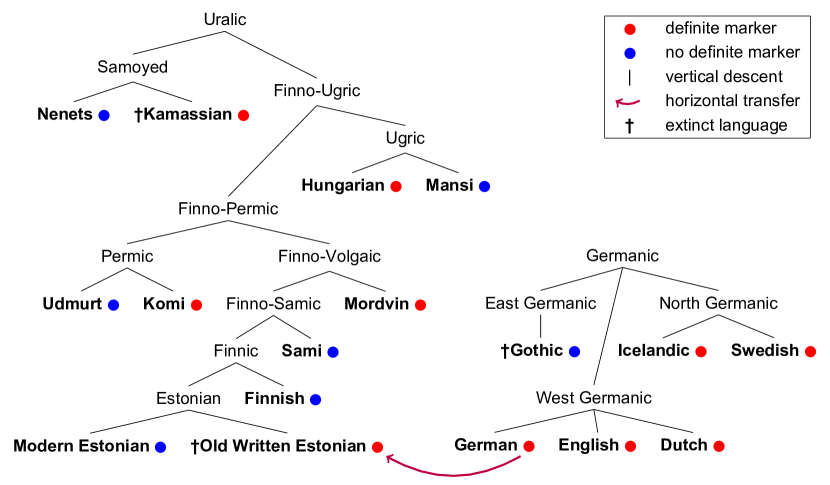
Figure 1: Some languages of the Uralic and Germanic families with respect to the presence of a definite marker (such as English the).

Secondly, genealogical stability estimation techniques necessarily miss out the effect of horizontal transfer—the borrowing of a feature from one family to another—on a feature’s stability. For example, Old Written Estonian was in extensive contact with German and borrowed a definite marker from it [21]; this relationship is visualized as the purple arrow in Fig. 1. The problem for genealogical stability estimation methods arises from the fact that some linguistic features (e.g. inflectional markers) are more resistant to horizontal transfer than others [22], while some (e.g. case systems) are highly vulnerable to simplification in contact situations involving large numbers of second-language learners [23]. Combining genealogical and areal groupings [11] is not a solution, however, as no agreed methods exist for delimiting linguistic areas or for estimating the time depths of areal relationships.

3 Stability estimation from geospatial distributions

The above criticisms motivate the search for a stability measure that reflects the relatedness of languages without presorting them into predefined groupings and can take horizontal transfer effects into account. Here, we propose such a technique by modelling language dynamics as a stochastic process on a spatial substrate; this model can be studied in computer simulations and mathematically. While the model dynamics continue indefinitely, the statistical properties of the distribution of features over physical space becomes stationary after the simulation has been run for a sufficiently long time. Using techniques from statistical physics, this stationary state can be characterized mathematically. In what follows, we show how this analytical solution can be utilized to estimate the tendency of individual linguistic features to change based solely on their contemporary geospatial distributions, measured from the WALS atlas [19].

Figure 2: Markov chain dynamics of a single linguistic feature. F: feature present; $-$F: feature absent.

Following an early but underexplored proposal of Greenberg’s [9], we treat the evolution of binary linguistic features as a memoryless stochastic process. The dynamics of each feature are then given by a Markov chain with two parameters, $p_{I}$ and $p_{E}$ (Fig. 2). The former parameter gives the probability of a language adopting the feature in question; we call it the feature’s ingress rate. The latter parameter, in turn, gives the probability of a language losing the feature; we will refer to it as the feature’s egress rate. We assume language communities to be distributed on a spatial substrate which, for reasons of mathematical tractability, we take to be a square lattice, i.e. language communities reside at regularly spaced positions over physical space. Each community is assumed to be subject to an ingress–egress dynamics as described by the Markov chain model of Fig. 2. To account for horizontal effects, we assume the existence of an interaction process between spatially contiguous language communities. This interaction process is based on the so-called voter model [24, 25, 26, 27, 28] and operates as follows. In each interaction event, a ‘target’ community is chosen, and the presence or absence of a feature in a randomly selected neighbouring community is copied into the target community. All in all, the model is iterated as follows:

1. Initialize the lattice in a random state (for each feature $F$ and community $C$, $F$ is present in $C$ with probability $0.5$).

2. Pick a random community $C$ and a random feature $F$.

3. Execute one of the following steps:

   1. with probability $q$: pick a random lattice neighbour $C^{\prime}$ of $C$, and set the value for feature $F$ in $C$ to that in $C^{\prime}$; or

   2. with probability $1-q$: if $F$ is absent from $C$, acquire $F$ with probability $p_{I}$ (ingress); if $F$ is present in $C$, lose $F$ with probability $p_{E}$ (egress).

4. Go to 2.

Inevitably, this model idealizes away from many of the complexities of real world language dynamics. What matters for present purposes is that the model should be able to capture two key elements contributing to language change. First, the evolution of a linguistic community over time is subject to both vertical and horizontal effects: the vertical effects arise mainly from the transmission of linguistic knowledge across generations through language acquisition; the horizontal effects reflect not only contact between speakers of different languages, but also contact between speakers of varieties of the same language [29]. Secondly, both vertical and horizontal effects can result in the faithful transmission of a feature or in a mutation. For example, contact between speakers of different languages can result in the simple transfer of a feature (borrowing), but it can also result in mutation, as when the interaction between two languages with different inflectional systems leads to the emergence of a simplified system that is different from both its predecessors [23]. In some instances of mutation, horizontal and vertical effects interact in highly intricate ways, e.g. during the formation of creole languages [30]. Our model reflects this state of affairs: faithful transmission occurs both vertically, with probability $(1-q)(1-p_{I}-p_{E})$, and horizontally, with probability $q$. In turn, the ingress–egress dynamics (probabilities $p_{I}$ and $p_{E}$) covers processes of mutation and is agnostic about their causes (vertical or horizontal).

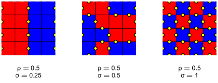
Figure 3: In the model, linguistic features evolve on a square lattice with periodic boundary conditions. The figure shows three ad hoc illustrations (red: feature present; blue: feature absent). In each case, the feature frequency is $\rho=0.5$ (half of the sites are blue, the other half are red). However, the isogloss density $\sigma$, defined as the proportion of disagreeing lattice interfaces (yellow dots), depends on the spatial distribution of the feature. It is low when a feature is present throughout extended domains, and larger when a feature is scattered.

The statistical properties of the stationary distribution of features at long times depends on the model parameters $p_{I}$, $p_{E}$ and $q$ (for further details see the SI). For the purposes of stability estimation, we are interested in two quantities in particular (illustrated in Fig. 3): the frequency, $\rho$, with which a particular feature is present across the lattice, and the feature’s associated isogloss density. This latter quantity indicates the probability of finding a dialect boundary (an isogloss) between two neighbouring communities such that the feature is found on one side of the boundary but not on the other. We define this as the proportion of pairs of adjacent lattice cells that differ in the feature value, and denote it by $\sigma$; similar quantities are sometimes also found as the ‘density of reactive interfaces’ in literature on interacting particle systems [25, 31]. The frequency of a feature in the stationary state is given by

$$\rho=\frac{p_{I}}{p_{I}+p_{E}}.$$ (1)

This can be demonstrated mathematically (see SI), but is also clear intuitively; the higher the ingress rate $p_{I}$ of a feature is in relation to its egress rate $p_{E}$, the more prevalent the feature will be. Obtaining the stationary isogloss density is more intricate mathematically (see again the SI). We find

$$\sigma=2H(\tau)\rho(1-\rho)$$ (2)

with

$$H(\tau)=\frac{\pi(1+\tau)}{2K\left(\frac{1}{1+\tau}\right)}-\tau$$ (3)

and

$$\tau=\frac{(1-q)(p_{I}+p_{E})}{q}.$$ (4)

The function $K(\cdot)$ denotes the complete elliptic integral of the first kind (see SI for full technical details). Thus, from Eq. (2), the stationary-state isogloss density $\sigma$ is found to be a parabolic function of the feature’s overall frequency $\rho$. The height of this parabola is controlled by the parameter $\tau$ (Fig. 4A); this parameter gives the relative rate of ingress–egress events (i.e., mutations) over faithful transmission (Eq. 4). For example, a value of $\tau=10^{-5}$ would indicate that faithful copying events between neighbouring communities are $10^{5}$ times more frequent on average than mutations. This suggests that $\tau$ can be interpreted as a temperature, measuring the amount of noise in the dynamics: lower values of $\tau$ signify a stable feature, higher values indicating instability.

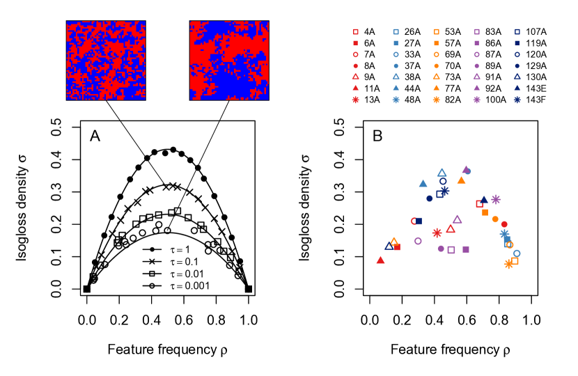
Figure 4: (A) Statistical properties of the model. At long times the state of the lattice is characterized by the two quantities feature frequency $\rho$ and isogloss density $\sigma$. We show computer simulations (markers) and analytical solution (curves) for different values of $\tau$ (determined by the combination of $p_{I}$, $p_{E}$ and $q$). Simulation snapshots are shown for two different values of $\tau$. (B) Empirical measurements of feature frequency $\rho$ and isogloss density $\sigma$ for 35 linguistic features, identified by their WALS feature IDs (see Methods for details).

We next describe how the above mathematical solution may be used to obtain estimates of the stability of linguistic features using contemporary geospatial data. Our particular aim is to estimate the temperature parameter $\tau$ for individual features, using geospatial information contained in the WALS database [19], focusing on 35 binary features (see Methods). For each feature, the frequency $\rho$ is given by the proportion of languages possessing that feature in the WALS language sample. The isogloss density $\sigma$ is calculated as follows: for each language, we first establish its nearest geographical neighbour in the relevant language sample. The empirical isogloss density is then given by the proportion of nearest-neighbour language pairs differing in their values for the feature in question. Our data are summarized in Fig. 4B, which supplies $\rho$ and $\sigma$ for each of the 35 features; a lower value of isogloss density $\sigma$ signals a geographically clustered feature, whilst a higher value implies a feature with a scattered geographical distribution. Fig. 5 illustrates this difference with two features, definite marker (WALS feature 37A) and order of object and verb (WALS feature 83A).

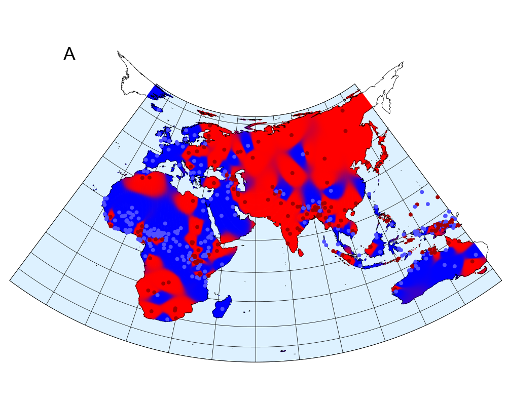
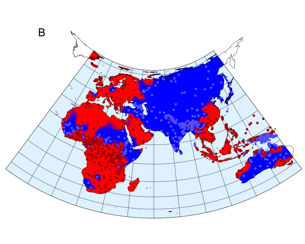
Figure 5: Empirical geospatial distributions of two linguistic features on the hemisphere from 30° W to 150° E (red: feature present, blue: feature absent): (A) definite marker (WALS feature 37A), (B) object–verb order (WALS feature 83A). Shown are both individual empirical data points (languages, as given by WALS coordinates) and a spatial interpolation (inverse distance weighting) on these points. Map projection: Albers equal-area.

For a given feature frequency $\rho$, the isogloss density $\sigma$ is fixed by the value of $H(\tau)$ (Eq. 2); this quantity itself is an increasing function of $\tau$ (Eq. 3). Since each of our 35 empirical features lies on a unique parabola in the space spanned by $\rho$ and $\sigma$ (Fig. 4), estimating its temperature is now a matter of inverting the function $H(\tau)$. For each feature, we measure $\rho$ and $\sigma$ as described above. From Eq. (2), we then obtain the value of $H(\tau)$ and invert this to recover $\tau$. Although the elliptic integral in Eq. (3) cannot be expressed in terms of elementary functions and $H(\tau)$ thus cannot be inverted analytically, the inversion can be performed numerically. Using this procedure we obtain an estimate of $\tau$ for any feature for which empirical measurements of frequency $\rho$ and isogloss density $\sigma$ exist. Table 1 supplies these estimates for the least stable and most stable features in our dataset (for a full listing of $\tau$ estimates for the entire dataset, see Table S2 in the SI).

Table 1: The seven least stable and most stable features in our dataset. Ranking is by decreasing temperature ($\tau$), as identified from WALS data using our model (see text).

Feature (WALS ID)	Temperature $\tau$
verbal person marking (100A)	$5.06\times 10^{-1}$
definite marker (37A)	$3.54\times 10^{-1}$
question particle (92A)	$3.43\times 10^{-1}$
gender in independent personal pronouns (44A)	$2.46\times 10^{-1}$
indefinite marker (38A)	$2.30\times 10^{-1}$
lateral consonants (8A)	$2.15\times 10^{-1}$
front rounded vowels (11A)	$1.95\times 10^{-1}$
$\vdots$	$\vdots$
velar nasal (9A)	$1.83\times 10^{-3}$
tone (13A)	$1.28\times 10^{-3}$
order of adjective and noun is AdjN (87A)	$1.21\times 10^{-3}$
order of subject and verb is SV (82A)	$4.93\times 10^{-4}$
order of genitive and noun is GenN (86A)	$3.34\times 10^{-5}$
order of numeral and noun is NumN (89A)	$3.31\times 10^{-5}$
order of object and verb is OV (83A)	$1.91\times 10^{-5}$

4 Comparison with a genealogical method

The technique proposed by Dediu [12] represents the state of the art in genealogy-based stability estimation. Using a Bayesian phylogenetic algorithm, this method produces a posterior distribution of rates of evolution for each linguistic feature within a predefined genealogical grouping. Dediu tests two phylogenetic algorithms and draws data from two sources—WALS and Ethnologue [32]—to control for implementation effects. His stability estimates are then expressed as the additive inverse of the first component (PC1) of a principal component analysis on the stability ranks predicted by each combination of phylogenetic algorithm and dataset (i.e. the higher the PC1 value, the less stable the feature).

In Fig. 6A, we consider the 24 features which are both in our list of 35 features and in Dediu’s list. Regressing our estimates for $\tau$ against Dediu’s PC1 (red regression line), we find a moderate correlation between the estimates predicted by the two methods (Pearson’s $r=0.53$, $p=0.008$). A number of features, however, are clearly outliers of the regression. To detect these outliers more objectively, we pruned the regression recursively by removing those data points that contribute the greatest error in terms of sum of squared residuals; Fig. 6B gives the reduction of error at each step of this pruning. The reduction profile prompts us to classify as outliers the first five data points, corresponding to the following WALS features: 11A (front rounded vowels), 107A (passive construction), 8A (lateral consonants), 44A (gender in independent personal pronouns) and 57A (possessive affixes). Regressing the pruned dataset (Fig. 6A, black regression line), we find a high correlation between our $\tau$ estimates and Dediu’s PC1 (Pearson’s $r=0.90$, $p=1.613\times 10^{-7}$).

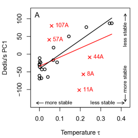
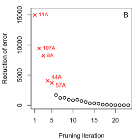
Figure 6: Regression of our temperature ($\tau$) estimates against Dediu’s PC1. (A) Red line: regression with all 24 data points (Pearson’s $r=0.53$, $p=0.008$). Black line: regression with five outliers (red crosses) removed (Pearson’s $r=0.90$, $p=1.613\times 10^{-7}$). (B) Outliers were detected by pruning the dataset recursively for those data points that contribute most to the regression error, quantified as the sum of squared residuals. This identified features 11A, 107A, 8A, 44A and 57A as outliers (see text).

We suggest that, rather than representing different views on stability, these outliers are false positives and negatives of the genealogical method. We illustrate this with the case of (the presence or absence of) front rounded vowels (WALS feature 11A), i.e. the vowels /y/ (e.g. Finnish kyy), /ø/ (German schön), /œ/ (French bœuf) and /Œ/ (Danish grøn). This is one of the most stable features in the genealogical analysis but one of the least stable features in ours (Table 1); we argue that evidence from both language change and language acquisition supports our position. On the one hand, front rounded vowels are frequently innovated: historical fronting of the back rounded vowel /u/ to [y] (with or without subsequent phonemicization to /y/) has been documented in a number of languages, including but not limited to Armenian, Attic-Ionic Greek, French, Frisian, Lithuanian, Old Scandinavian, Oscan, Parachi, Umbrian, West Syriac, Yiddish, Zuberoan Basque, and numerous dialects of English [33, 34, 35, 36, 37, 38, 39]; additionally, front rounded vowels can arise through the influence of /i/ or /j/ on a neighbouring back rounded vowel [33, 40]. On the other hand, front rounded vowels are difficult to acquire in situations of language contact: there is experimental evidence that second-language learners whose first language lacks these vowels perceive them as more similar to back vowels than front vowels [41]. This perceptual assimilation is mirrored in speech production: productions of /y/ by second-language learners are far less advanced in phonetic space than native speakers’ productions, and are indeed often perceived as /u/ by the latter [42]. The fact that front rounded vowels are readily innovated points to a high ingress rate, while frequent acquisition failure by second-language learners in situations of language contact points to a high egress rate. These facts are inconsistent with the high stability predicted by the genealogical method, but consistent with our approach, in which high ingress and high egress make for high temperature (Eq. 4) and thus low stability.

Although space limitations preclude a full linguistic analysis, we point out that similar arguments can be made for the remaining outliers. For instance, all Uralic languages employ possessive affixes (e.g. Finnish auto-ni ‘my car’, auto-si ‘your car’, etc.), and the appearance of this system of possession can be dated back to Pre-Proto-Uralic by standard reconstructive techniques [43]. Possessive affixes are also old in the unrelated Turkic language family [44]. There is, then, reason to believe that WALS feature 57A on possessive affixes is a false negative of the genealogical method, which classifies possessive affixes as one of the least stable features (Fig. 6).

5 Discussion

The challenge of linguistic stability estimation arises, essentially, from having to work with a poor signal. Although evolutionary and anthropological evidence suggests that human language in its modern form has existed for at least 100,000 years [45, 46], the historical evolution of languages is (necessarily) poorly documented. Such documentation only captures a few thousand years for languages with the best coverage, cannot in principle go beyond the introduction of the first writing systems, and does not exist at all for the majority of the world’s languages. The rest of the historical evolution of language must be reconstructed based on available data. In this paper, we have argued that stability estimation methods relying on even the most accurate reconstructive methods have their shortcomings: there is no guarantee that the genealogical classifications assumed in such estimation reflect equivalent time depths between different language families, and the methods do not control for horizontal transfer between languages belonging to different families. We have introduced a stability estimation procedure that does without genealogies and infers stability estimates from contemporary geospatial distributions of linguistic features alone. The method is relatively easy to implement: all that is needed are measures of feature frequency and isogloss density for a large enough sample of languages, and inversion of Eq. (3).

We have offered some evidence in support of our method, in the sense that this method is not liable to some of the false positives and false negatives incurred by genealogical methods. Turning now to its limitations, we note that our approach currently only applies to binary features, i.e. features which are either present in or absent from a language community. Most genealogical methods do not suffer from this limitation: Dediu’s [12] procedure, in particular, can be applied to polyvalent as well as binary features. Interestingly, however, Dediu finds a correlation between estimates generated for polyvalent and binary (or binarized) features. This suggests that the resolution at which the values of a linguistic variable are recorded may be a minor issue: after all, any polyvalent classification can be reduced to a hierarchy of binary oppositions. Another limitation of our technique, shared by all existing methods, is that it treats the evolution of individual features independently of the rest. Feature interactions are known to exist, however—for example, a language which places objects before verbs is far more likely to also place adverbs before verbs, rather than after them [47, 48]. It is in principle possible to generalize our method to cater for polyvalent features and feature interactions, by extending the lattice model in the direction of the Axelrod model of cultural dissemination [49]. It is at the moment unclear, however, whether the behaviour of such a generalized model can be solved analytically so that stability estimates may be derived in the way we have described.

While these remain tasks for future research, the present study enables us to conclude that, though hitherto underexploited, geospatial distributions provide one of the best sources of evidence on the rates of evolution of features of human language.

Methods

Data preparation

The WALS Online database [19] was downloaded on 18 July 2017 and used as the empirical basis for measures of feature frequency $\rho$ and isogloss density $\sigma$. Since WALS employs a polyvalent coding for most features, a manual pass was made, retaining only those features that are binary or binarizable on uncontroversial linguistic grounds. Features with fewer than 300 languages in their language sample were discarded to ensure statistically robust results. This procedure resulted in 35 binary features (see Table S1 in the SI for a listing, together with full information about our binarization scheme). Nearest neighbours of languages were determined by the great-circle distance, calculated from WALS coordinate data using the haversine formula with the assumption of a perfectly spherical earth.

Analysis

To eliminate any possible effect the differing language sample sizes of different WALS features might have on our statistics, a fixed number of 300 languages was considered for each feature, with languages sampled uniformly at random from the feature’s language sample. This procedure was repeated 10,000 times for each feature to generate the bootstrap averages reported in Fig. 4B. For comparison with the genealogical method, Table S1 in the SI to Ref. [12] was consulted and only those features were selected for comparison for which our binarization schemes agreed; the PC1 values for the intersecting features were then gathered from Table S4. Correlation strengths were measured using the Pearson correlation coefficient; significance was tested with a two-tailed $t$-test. The analytical solution of the lattice model (Eqs. 1–3) appears in the SI.

Data availability

WALS is freely available at http://wals.info; the binarization scheme used to prepare the data appears in the SI.

Code availability

Computer code for data analysis, stability estimation and numerical simulations may be obtained from the corresponding author.

Author contributions

Designed the study: HK, DG, TG and RB-O. Analysed the data: HK, DG, TG and RB-O. Solved the mathematical model: HK, DG and TG. Wrote the paper: HK, DG, TG and RB-O. Wrote visualization routines: HK and DG. Wrote the data analysis and simulation code: HK.

Author information

The authors declare no conflict of interest and no competing financial interests. Correspondence and requests for materials should be addressed to henri.kauhanen@uni-konstanz.de.

Appendix A Features consulted

Table S1 provides a listing of the 35 WALS [19] features consulted in this study, together with our scheme for feature binarization. Each WALS feature is a variable of either nominal or ordinal level, whose possible values are recorded in the WALS database using integer labels. The meanings of these labels are explained at length in Section D, below; Table S1 indicates which values of each variable were folded into the ‘feature absent’ category and which values to the ‘feature present’ category in our binarization.

Table S1: The 35 binary features considered in this study. The ‘WALS’ column gives the WALS feature mined; values indicated in the ‘abs.’ column were folded into our ‘binary feature absent’ value, whilst values indicated in the ‘pres.’ column were folded into our ‘binary feature present’ value (see Section D, below). The final column gives the size of the WALS language sample (number of languages) for each feature.

	description	WALS	abs.	pres.	$N$
1.	adpositions	48A	1	2–4	378
2.	definite marker	37A	4–5	1–3	620
3.	hand and arm identical	129A	2	1	617
4.	hand and finger(s) identical	130A	2	1	593
5.	front rounded vowels	11A	1	2–4	562
6.	gender in independent personal pronouns	44A	6	1–5	378
7.	glottalized consonants	7A	1	2–8	567
8.	grammatical evidentials	77A	1	2–3	418
9.	indefinite marker	38A	4–5	1–3	534
10.	inflectional morphology	26A	1	2–6	969
11.	inflectional optative	73A	2	1	319
12.	lateral consonants	8A	1	2–5	567
13.	morphological second-person imperative	70A	5	1–4	547
14.	order of adjective and noun is AdjN	87A	2	1	1366
15.	order of degree word and adjective is DegAdj	91A	2	1	481
16.	order of genitive and noun is GenN	86A	2	1	1249
17.	order of numeral and noun is NumN	89A	2	1	1153
18.	order of object and verb is OV	83A	2	1	1519
19.	order of subject and verb is SV	82A	2	1	1497
20.	ordinal numerals	53A	1	2–8	321
21.	passive construction	107A	2	1	373
22.	plural	33A	9	1–8	1066
23.	possessive affixes	57A	4	1–3	902
24.	postverbal negative morpheme	143F	4	1–3	1324
25.	preverbal negative morpheme	143E	4	1–3	1324
26.	productive reduplication	27A	3	1–2	368
27.	question particle	92A	6	1–5	884
28.	shared encoding of nominal and locational predication	119A	1	2	386
29.	tense-aspect inflection	69A	5	1–4	1131
30.	tone	13A	1	2–3	527
31.	uvular consonants	6A	1	2–4	567
32.	velar nasal	9A	3	1–2	469
33.	verbal person marking	100A	1	2–6	380
34.	voicing contrast	4A	1	2–4	567
35.	zero copula for predicate nominals	120A	1	2	386

Appendix B Temperature estimates

Table S2 gives the temperature ($\tau$) estimates found by our method for the 35 features.

Table S2: Feature frequency $\rho$, isogloss density $\sigma$ and estimated temperature $\tau$ for the 35 features considered in this study (to eight significant decimals), ordered by increasing $\tau$ (from stable to unstable).

	feature	$\rho$	$\sigma$	$\tau$
1.	order of object and verb is OV	0.50352113	0.12087912	0.00001910
2.	order of numeral and noun is NumN	0.44097222	0.12454212	0.00003306
3.	order of genitive and noun is GenN	0.59420290	0.12204724	0.00003339
4.	order of subject and verb is SV	0.86071429	0.07722008	0.00049325
5.	order of adjective and noun is AdjN	0.29856115	0.14843750	0.00120923
6.	tone	0.41666667	0.17333333	0.00128340
7.	velar nasal	0.50000000	0.18333333	0.00183200
8.	order of degree word and adjective is DegAdj	0.54135338	0.21212121	0.00569870
9.	uvular consonants	0.17000000	0.13000000	0.00979939
10.	ordinal numerals	0.89666667	0.08666667	0.01181972
11.	shared encoding of nominal and locational predication	0.30333333	0.21000000	0.01732702
12.	glottalized consonants	0.27666667	0.21000000	0.02605203
13.	inflectional optative	0.15000000	0.14333333	0.04120610
14.	inflectional morphology	0.85333333	0.14000000	0.04215630
15.	possessive affixes	0.71333333	0.23666667	0.04784846
16.	passive construction	0.43333333	0.29333333	0.05949459
17.	tense-aspect inflection	0.86666667	0.13666667	0.05994843
18.	hand and arm identical	0.37000000	0.28000000	0.06211254
19.	productive reduplication	0.85000000	0.15333333	0.06274509
20.	voicing contrast	0.68000000	0.26333333	0.06769913
21.	adpositions	0.83333333	0.17000000	0.06908503
22.	postverbal negative morpheme	0.46333333	0.30333333	0.06961203
23.	hand and finger(s) identical	0.12000000	0.13000000	0.07032095
24.	morphological second-person imperative	0.77666667	0.21666667	0.08655531
25.	preverbal negative morpheme	0.70666667	0.27333333	0.11292895
26.	plural	0.91000000	0.11000000	0.12817720
27.	zero copula for predicate nominals	0.45333333	0.33333333	0.13213325
28.	grammatical evidentials	0.56666667	0.33333333	0.14401769
29.	front rounded vowels	0.06666667	0.08666667	0.19468340
30.	lateral consonants	0.83333333	0.20000000	0.21489842
31.	indefinite marker	0.44666667	0.35666667	0.22952822
32.	gender in independent personal pronouns	0.33000000	0.32333333	0.24577576
33.	question particle	0.59666667	0.36666667	0.34336306
34.	definite marker	0.60666667	0.36333333	0.35396058
35.	verbal person marking	0.78000000	0.27666667	0.50590667

Appendix C Analytical solution of lattice model

We will treat the model as a spin system on a two-dimensional regular square lattice with $N=L\times L$ sites and periodic boundary conditions (for comparable approaches to the voter model without an ingress–egress dynamics, see Refs. [25, 31]). Our model is conceptually similar to a voter model with noise, which has been treated with similar methods in Ref. [50]. We write $s(\mathbf{x})\in\{-1,1\}$ for the spin at lattice site $\mathbf{x}=(x_{1},x_{2})$; $S(\mathbf{x})=\langle s(\mathbf{x})\rangle$ for the average spin of $\mathbf{x}$ (over realizations of the stochastic process); and $m=\sum_{\mathbf{x}}S(\mathbf{x})/N$ for the mean magnetization over the entire lattice. The feature frequency $\rho$, or fraction of up-spins in the system, is related to $m$ by the identity $\rho=(m+1)/2$. We further write $S(\mathbf{x},\mathbf{y})=\langle s(\mathbf{x})s(\mathbf{y})\rangle$ for the pair correlation of $s(\mathbf{x})$ and $s(\mathbf{y})$. In summations, $\mathbf{x}^{\prime}$ is understood to index the set of von Neumann neighbours of site $\mathbf{x}$, i.e. the set

$$\{(x_{1}-1,x_{2}),(x_{1}+1,x_{2}),(x_{1},x_{2}-1),(x_{1},x_{2}+1)\}.$$ (S1)

C.1 Spin flip probability

Central to our analytical derivations is the spin flip probability, i.e. the probability with which the spin at site $\mathbf{x}$ changes its state from $-1$ to $+1$ or vice versa, if it is selected for potential update. In our model this is of the form

$$w(\mathbf{x})=(1-q)A(\mathbf{x})+qB(\mathbf{x}),$$ (S2)

where $A(\mathbf{x})$ is the contribution of the ingress–egress process and $B(\mathbf{x})$ the contribution of the spatial (voter) process. These are

$$A(\mathbf{x})=\frac{1-s(\mathbf{x})}{2}p_{I}+\frac{1+s(\mathbf{x})}{2}p_{E}=\frac{1}{2}\left[p_{I}+p_{E}+(p_{E}-p_{I})s(\mathbf{x})\right]$$ (S3)

and

$$B(\mathbf{x})=\frac{1}{4}\sum_{\mathbf{x}^{\prime}}\frac{1-s(\mathbf{x})s(\mathbf{x}^{\prime})}{2}=\frac{1}{2}\left[1-\frac{1}{4}\sum_{\mathbf{x}^{\prime}}s(\mathbf{x})s(\mathbf{x}^{\prime})\right],$$ (S4)

where it is important to remember that the summation over $\mathbf{x}^{\prime}$ runs over the four nearest neighbours of $\mathbf{x}$. Hence we have

$$w(\mathbf{x})=\frac{1-q}{2}\left[p_{I}+p_{E}+(p_{E}-p_{I})s(\mathbf{x})\right]+\frac{q}{2}\left[1-\frac{1}{4}\sum_{\mathbf{x}^{\prime}}s(\mathbf{x})s(\mathbf{x}^{\prime})\right].$$ (S5)

C.2 Stationary-state feature frequency $\rho$

The spin at $\mathbf{x}$ changes by the amount $-2s(\mathbf{x})$ with probability $\frac{1}{N}w(\mathbf{x})$, the prefactor $1/N$ representing the probability of $\mathbf{x}$ being picked for update. Consequently, the mean spin $S(\mathbf{x})=\langle s(\mathbf{x})\rangle$ evolves as

$$S(\mathbf{x},t+\Delta t)-S(\mathbf{x},t)=\frac{1}{N}\langle-2w(\mathbf{x})s(\mathbf{x})\rangle,$$ (S6)

where $\Delta t$ is the time step associated with each attempted spin flip. Bearing in mind that $s(\mathbf{x})s(\mathbf{x})=1$ and plugging Eq. (S5) in, this implies

$$\frac{S(\mathbf{x},t+\Delta t)-S(\mathbf{x},t)}{1/N}=(1-q)\left[p_{I}-p_{E}-(p_{I}+p_{E})S(\mathbf{x})\right]+q\left[-S(\mathbf{x})+\frac{1}{4}\sum_{\mathbf{x}^{\prime}}S(\mathbf{x}^{\prime})\right].$$ (S7)

Taking the sum over all sites $\mathbf{x}$, one has

$$\begin{split}\frac{m(t+\Delta t)-m(t)}{1/N}&=(1-q)(p_{I}-p_{E})-(1-q)(p_{I}+p_{E})\frac{1}{N}\sum_{\mathbf{x}}S(\mathbf{x})-\\ &\quad\quad-\frac{q}{N}\sum_{\mathbf{x}}S(\mathbf{x})+\frac{q}{4N}\sum_{\mathbf{x}}\sum_{\mathbf{x}^{\prime}}S(\mathbf{x}^{\prime}).\end{split}$$ (S8)

Now $\sum_{\mathbf{x}}\sum_{\mathbf{x}^{\prime}}S(\mathbf{x}^{\prime})=4\sum_{\mathbf{x}}S(\mathbf{x})$, since the LHS is the sum of the four von Neumann neighbours of all lattice sites, so that each site, having four neighbours, gets counted four times. Using $m=\sum_{\mathbf{x}}S(\mathbf{x})/N$, we then have

$$\frac{m(t+\Delta t)-m(t)}{1/N}=(1-q)\left[p_{I}-p_{E}-(p_{I}+p_{E})m\right].$$ (S9)

With the standard choice $\Delta t=1/N$, and taking the limit $N\to\infty$ (i.e. the continuous-time limit $\Delta t\to 0$), we thus find

$$\frac{dm}{dt}=(1-q)\left[p_{I}-p_{E}-(p_{I}+p_{E})m\right].$$ (S10)

Hence the mean magnetization in the stationary state ($dm/dt=0$) is

$$m=\frac{p_{I}-p_{E}}{p_{I}+p_{E}}.$$ (S11)

From this, using $\rho=(m+1)/2$, we find

$$\rho=\frac{p_{I}}{p_{I}+p_{E}}$$ (S12)

for the fraction of up-spins in the stationary state.

C.3 Pair correlation function

To compute the pair correlation $S(\mathbf{x},\mathbf{y})=\langle s(\mathbf{x})s(\mathbf{y})\rangle$, we note that $s(\mathbf{x})s(\mathbf{y})$ changes by the amount $-2s(\mathbf{x})(\mathbf{y})$ if either $\mathbf{x}$ or $\mathbf{y}$ flips spin. Assuming $\mathbf{x}\neq\mathbf{y}$, and working directly in the continuous-time limit, we have

$$\frac{dS(\mathbf{x},\mathbf{y})}{dt}=\langle-2\left[w(\mathbf{x})+w(\mathbf{y})\right]s(\mathbf{x})s(\mathbf{y})\rangle.$$ (S13)

After some algebra we find

$$\begin{split}\frac{dS(\mathbf{x},\mathbf{y})}{dt}&=(1-q)\left[(p_{I}-p_{E})[S(\mathbf{x})+S(\mathbf{y})]-2(p_{I}+p_{E})S(\mathbf{x},\mathbf{y})\right]+\\ &\quad\quad+q\left[-2S(\mathbf{x},\mathbf{y})+\frac{1}{4}\sum_{\mathbf{x}^{\prime}}S(\mathbf{x}^{\prime},\mathbf{y})+\frac{1}{4}\sum_{\mathbf{y}^{\prime}}S(\mathbf{x},\mathbf{y}^{\prime})\right],\end{split}$$ (S14)

where the summation over $\mathbf{y}^{\prime}$ is over the four nearest neighbours of $\mathbf{y}$.

We now assume translation invariance and write $C(\mathbf{r})=C(\mathbf{x}-\mathbf{y})=S(\mathbf{x},\mathbf{y})$. Then, for $\mathbf{r}\neq\mathbf{0}$,

$$\begin{split}\frac{dC(\mathbf{r})}{dt}&=(1-q)\left[(p_{I}-p_{E})[S(\mathbf{x})+S(\mathbf{y})]-2(p_{I}+p_{E})C(\mathbf{r})\right]+\\ &\quad\quad+q\left[-2C(\mathbf{r})+\frac{1}{4}\sum_{\mathbf{x}^{\prime}}C(\mathbf{x}^{\prime}-\mathbf{y})+\frac{1}{4}\sum_{\mathbf{y}^{\prime}}C(\mathbf{x}-\mathbf{y}^{\prime})\right].\end{split}$$ (S15)

Due to translation invariance the two summations on the RHS coincide, and we have (always restricting $\mathbf{r}\neq\mathbf{0}$)

$$\frac{dC(\mathbf{r})}{dt}=(1-q)\left[(p_{I}-p_{E})[S(\mathbf{x})+S(\mathbf{y})]-2(p_{I}+p_{E})C(\mathbf{r})\right]+2q\Delta C(\mathbf{r}),$$ (S16)

where $\Delta$ is the lattice Laplace operator

$$\Delta f(\mathbf{x})=-f(\mathbf{x})+\frac{1}{4}\sum_{\mathbf{x}^{\prime}}f(\mathbf{x}^{\prime}).$$ (S17)

We note that we always have the boundary condition $C(\mathbf{0},t)=1$ for all $t$ (self-correlation is $1$ at all times, as $s(\mathbf{x})^{2}=1$).

C.4 Stationary-state isogloss density $\sigma$

If $C(\mathbf{e}_{1},t)$ were known, where $\mathbf{e}_{1}$ is the unit vector $(1,0)$, the isogloss density could be obtained via the identity

$$\sigma(t)=\frac{1-C(\mathbf{e}_{1},t)}{2}.$$ (S18)

Thus, knowing the limiting ($t\to\infty$) value of $C(\mathbf{e}_{1})$ would imply the stationary-state isogloss density $\sigma$.

At the stationary state, $S(\mathbf{x})+S(\mathbf{y})=2m$ and $\frac{dC(\mathbf{r})}{dt}=0$. Assuming $\mathbf{r}\neq\mathbf{0}$, Eq. (S16) then implies

$$0=(1-q)\left[2(p_{I}-p_{E})m-2(p_{I}+p_{E})C(\mathbf{r})\right]+2q\Delta C(\mathbf{r}),$$ (S19)

in other words,

$$\begin{split}0&=(1-q)\left[(p_{I}-p_{E})m-(p_{I}+p_{E})C(\mathbf{r})\right]+q\Delta C(\mathbf{r})\\ &=(1-q)(p_{I}+p_{E})\left[\frac{p_{I}-p_{E}}{p_{I}+p_{E}}m-C(\mathbf{r})\right]+q\Delta C(\mathbf{r})\\ &=(1-q)(p_{I}+p_{E})\left[m^{2}-C(\mathbf{r})\right]+q\Delta C(\mathbf{r}).\end{split}$$ (S20)

In the special case $q=0$ (i.e., no spatial interaction between neighbouring sites), this implies $C(\mathbf{r})=m^{2}$ for all $\mathbf{r}\neq\mathbf{0}$. Thus for any two sites $\mathbf{x}\neq\mathbf{y}$, $\langle s(\mathbf{x})s(\mathbf{y})\rangle=m^{2}$, indicating that spins at different sites are fully uncorrelated. This is what one would expect, as all sites operate independently when $q=0$.

In the special case $q=1$ (no ingress–egress dynamics within the sites), on the other hand, we obtain $\Delta C(\mathbf{r})=0$ for $\mathbf{r}\neq 0$. We also have $C(\mathbf{0})=0$. This implies $C(\mathbf{r})=1$ everywhere, so either all spins are up or all are down. This is the only possible stationary state when the only dynamics is through nearest-neighbour interactions.

Now suppose $0<q<1$. Dividing Eq. (S20) by $q$ we obtain

$$\begin{split}0&=\frac{1-q}{q}(p_{I}+p_{E})\left[m^{2}-C(\mathbf{r})\right]+\Delta C(\mathbf{r})\\ &=\frac{(q-1)(p_{I}+p_{E})}{q}\left[C(\mathbf{r})-m^{2}\right]+\Delta C(\mathbf{r})\\ &=\alpha C(\mathbf{r})-\alpha m^{2}+\Delta C(\mathbf{r}),\end{split}$$ (S21)

where we write

$$\alpha=\frac{(q-1)(p_{I}+p_{E})}{q}.$$ (S22)

Now let

$$c(\mathbf{r})=C(\mathbf{r})-m^{2}.$$ (S23)

We note that $\Delta C(\mathbf{r})=\Delta c(\mathbf{r})$. To solve Eq. (S21), it then suffices to solve (for $\mathbf{r}\neq\mathbf{0}$)

$$\Delta c(\mathbf{r})+\alpha c(\mathbf{r})=0$$ (S24)

subject to the condition

$$c(\mathbf{0})=1-m^{2}.$$ (S25)

We now first focus on the equation

$$\Delta G(\mathbf{r})+\alpha G(\mathbf{r})=-\delta_{\mathbf{r},\mathbf{0}},$$ (S26)

for all $\mathbf{r}$ (including $\mathbf{r}=\mathbf{0}$), and where $\delta_{\mathbf{x},\mathbf{y}}$ is the Kronecker delta.

Let $G_{\alpha}(\mathbf{r})$ be a solution of Eq. (S26). Then

$$c(\mathbf{r})=(1-m^{2})\frac{G_{\alpha}(\mathbf{r})}{G_{\alpha}(\mathbf{0})}$$ (S27)

is a solution of Eqs. (S24) and (S25). This can be seen as follows: first, from Eq. (S27),

$$c(\mathbf{0})=(1-m^{2})\frac{G_{\alpha}(\mathbf{0})}{G_{\alpha}(\mathbf{0})}=1-m^{2},$$ (S28)

so the condition in Eq. (S25) is met. Second, we need to show that Eqs. (S26) and (S27) imply $\Delta c(\mathbf{r})+\alpha c(\mathbf{r})=0$ for $\mathbf{r}\neq\mathbf{0}$. For $\mathbf{r}\neq\mathbf{0}$ we have

$$\Delta G(\mathbf{r})+\alpha G(\mathbf{r})=0$$ (S29)

from Eq. (S26). The quantity $c(\mathbf{r})$ in Eq. (S27) is proportional to $G_{\alpha}(\mathbf{r})$ with a proportionality constant $(1-m^{2})/G_{\alpha}(\mathbf{0})$ which is independent of $\mathbf{r}$. Given that $G_{\alpha}(\mathbf{r})$ fulfills Eq. (S29) for $\mathbf{r}\neq\mathbf{0}$ it is then clear that $c(\mathbf{r})$ fulfills $\Delta c(\mathbf{r})+\alpha c(\mathbf{r})=0$ for $\mathbf{r}\neq\mathbf{0}$, i.e. Eq. (S24).

So we are left with the task of finding a solution of

$$\Delta G(\mathbf{r})+\alpha G(\mathbf{r})=-\delta_{\mathbf{r},\mathbf{0}}.$$ (S30)

Let us write $G(\mathbf{r})$ in Fourier representation:

$$G(\mathbf{r})=\frac{1}{(2\pi)^{2}}\int_{-\pi}^{\pi}\int_{-\pi}^{\pi}dk_{1}dk_{2}\leavevmode\nobreak\ e^{i\mathbf{k}\cdot\mathbf{r}}\widehat{G}(\mathbf{k}),$$ (S31)

where $\mathbf{k}=(k_{1},k_{2})$ and $\widehat{G}(\mathbf{k})$ is the Fourier transform of $G(\mathbf{r})$, i.e.

$$\widehat{G}(\mathbf{k})=\sum_{\mathbf{r}}e^{-i\mathbf{k}\cdot\mathbf{r}}G(\mathbf{r})=\sum_{x}\sum_{y}e^{-ixk_{1}-iyk_{2}}G(x,y).$$ (S32)

Applying this to both sides of Eq. (S30) leads to

$$\sum_{x,y}e^{-ixk_{1}-iyk_{2}}\left[\Delta G(\mathbf{r})+\alpha G(\mathbf{r})\right]=-1.$$ (S33)

Next, notice

$$\begin{split}\sum_{x,y}e^{-ixk_{1}-iyk_{2}}\Delta G(x,y)&=\frac{1}{4}\sum_{x,y}e^{-ixk_{1}-iyk_{2}}\left[G(x+1,y)+G(x-1,y)\right.+\\ &\quad\quad\left.+G(x,y+1)+G(x,y-1)-4G(x,y)\right]\\ &=\frac{1}{4}\sum_{x,y}\left[e^{-i(x-1)k_{1}-iyk_{2}}+e^{-i(x+1)k_{1}-iyk_{2}}\right.+\\ &\quad\quad\left.+e^{-ixk_{1}-i(y-1)k_{2}}+e^{-ixk_{1}-i(y+1)k_{2}}-4e^{-ixk_{1}-iyk_{2}}\right]G(x,y)\\ &=\frac{1}{4}\sum_{x,y}\left[\underbrace{e^{ik_{1}}+e^{-ik_{1}}}_{=2\cos k_{1}}+\underbrace{e^{ik_{2}}+e^{-ik_{2}}}_{=2\cos k_{2}}-4\right]e^{-ixk_{1}-iyk_{2}}G(x,y)\\ &=\frac{1}{2}\left[\cos k_{1}+\cos k_{2}-2\right]\sum_{x,y}e^{-ixk_{1}-iyk_{2}}G(x,y)\\ &=\frac{1}{2}\left[\cos k_{1}+\cos k_{2}-2\right]\widehat{G}(\mathbf{k}).\end{split}$$ (S34)

Using this in Eq. (S33) gives

$$\left[\frac{1}{2}\left(\cos k_{1}+\cos k_{2}-2\right)+\alpha\right]\widehat{G}(\mathbf{k})=-1,$$ (S35)

in other words

$$\widehat{G}(\mathbf{k})=\frac{1}{1-\alpha-\frac{1}{2}\left[\cos k_{1}+\cos k_{2}\right]}.$$ (S36)

Using Eq. (S31) we then have

$$G_{\alpha}(\mathbf{r})=\frac{1}{(2\pi)^{2}}\int_{-\pi}^{\pi}\int_{-\pi}^{\pi}\frac{e^{i\mathbf{k}\cdot\mathbf{r}}dk_{1}dk_{2}}{1-\alpha-\frac{1}{2}(\cos k_{1}+\cos k_{2})}.$$ (S37)

Hence

$$G_{\alpha}(\mathbf{0})=\frac{1}{(2\pi)^{2}}\int_{-\pi}^{\pi}\int_{-\pi}^{\pi}\frac{dk_{1}dk_{2}}{1-\alpha-\frac{1}{2}(\cos k_{1}+\cos k_{2})}.$$ (S38)

The integrand is symmetric with respect to $k_{1}\leftrightarrow-k_{1}$ and $k_{2}\leftrightarrow-k_{2}$ respectively, due to the identity $\cos(k)=\cos(-k)$. Hence

$$\begin{split}G_{\alpha}(\mathbf{0})&=\frac{1}{\pi^{2}}\int_{0}^{\pi}\int_{0}^{\pi}\frac{dk_{1}dk_{2}}{1-\alpha-\frac{1}{2}(\cos k_{1}+\cos k_{2})}\\ &=\frac{1}{1-\alpha}\frac{1}{\pi^{2}}\int_{0}^{\pi}\int_{0}^{\pi}\frac{dk_{1}dk_{2}}{1-\frac{1}{2(1-\alpha)}(\cos k_{1}+\cos k_{2})}.\end{split}$$ (S39)

This expression is related to the complete elliptic integral of the first kind, see for example Ref. [51]. We use the following notation:

$$K(z)=\frac{1}{2\pi}\int_{0}^{\pi}du\int_{0}^{\pi}dv\frac{1}{1-\frac{z}{2}(\cos u+\cos v)}.$$ (S40)

Hence we have

$$G_{\alpha}(\mathbf{0})=\frac{2}{\pi(1-\alpha)}K\left(\frac{1}{1-\alpha}\right)=\frac{2K_{\alpha}}{\pi(1-\alpha)},$$ (S41)

where we abbreviate

$$K_{\alpha}=K\left(\frac{1}{1-\alpha}\right)$$ (S42)

for convenience.

Next, we write the Laplacian $\Delta G_{\alpha}(\mathbf{0})$ in full:

$$\Delta G_{\alpha}(\mathbf{0})=-G_{\alpha}(\mathbf{0})+\frac{1}{4}[G_{\alpha}(1,0)+G_{\alpha}(-1,0)+G_{\alpha}(0,1)+G_{\alpha}(0,-1)].$$ (S43)

Assuming isotropy, each term in the square brackets is equal to $G_{\alpha}(\mathbf{e}_{1})=G_{\alpha}(1,0)$. Hence Eq. (S30), evaluated at $\mathbf{r}=\mathbf{0}$, takes the form

$$G_{\alpha}(\mathbf{e}_{1})+(\alpha-1)G_{\alpha}(\mathbf{0})=-1,$$ (S44)

in other words

$$G_{\alpha}(\mathbf{0})-G_{\alpha}(\mathbf{e}_{1})=1+\alpha G_{\alpha}(\mathbf{0}).$$ (S45)

From this we find

$$1-\frac{G_{\alpha}(\mathbf{e}_{1})}{G_{\alpha}(\mathbf{0})}=\left[\alpha+\frac{1}{G_{\alpha}(\mathbf{0})}\right].$$ (S46)

Now using Eqs. (S23) and (S27),

$$C(\mathbf{r})=m^{2}+c(\mathbf{r})=m^{2}+(1-m^{2})\frac{G_{\alpha}(\mathbf{r})}{G_{\alpha}(\mathbf{0})}.$$ (S47)

The stationary-state isogloss density $\sigma$ is then

$$\begin{split}\sigma&=\frac{1}{2}[1-C(\mathbf{e}_{1})]\\ &=\frac{1}{2}\left[1-m^{2}-(1-m^{2})\frac{G_{\alpha}(\mathbf{e}_{1})}{G_{\alpha}(\mathbf{0})}\right]\\ &=\frac{1}{2}(1-m^{2})\left[1-\frac{G_{\alpha}(\mathbf{e}_{1})}{G_{\alpha}(\mathbf{0})}\right]\\ &=\frac{1}{2}(1-m^{2})\left[\alpha+\frac{1}{G_{\alpha}(\mathbf{0})}\right]\\ &=\frac{1}{2}(1-m^{2})\left[\alpha+\frac{\pi(1-\alpha)}{2K_{\alpha}}\right],\end{split}$$ (S48)

where we have used Eq. (S41). On the other hand,

$$1-m^{2}=1-\frac{(p_{I}-p_{E})^{2}}{(p_{I}+p_{E})^{2}}=4\left(\frac{p_{I}}{p_{I}+p_{E}}\right)\left(\frac{p_{E}}{p_{I}+p_{E}}\right)=4\rho(1-\rho),$$ (S49)

so that

$$\sigma=2\rho(1-\rho)\left[\alpha+\frac{\pi(1-\alpha)}{2K_{\alpha}}\right].$$ (S50)

Recalling that

$$\alpha=-\tau=-\frac{(1-q)(p_{I}+p_{E})}{q},$$ (S51)

see Eq. (S22), and defining $\tau=-\alpha$, i.e. $K_{\alpha}=K_{-\tau}$, yields our final equation for the stationary-state isogloss density:

$$\sigma=2H(\tau)\rho(1-\rho),$$ (S52)

where

$$H(\tau)=\frac{\pi(1+\tau)}{2K\left(\frac{1}{1+\tau}\right)}-\tau.$$ (S53)

The expression in Eq. (S52) is a downward-opening parabola in $\rho$ whose height is fixed by $H(\tau)$, where

$$\tau=\frac{(1-q)(p_{I}+p_{E})}{q}.$$ (S54)

C.5 Sanity check: the limits $\tau\to 0$ and $\tau\to\infty$

The complete elliptic integral $K(z)$ has the following known properties [52]:

$$\lim_{z\to 0}K(z)=\frac{\pi}{2}\quad\textnormal{and}\quad\lim_{z\to 1}K(z)=\infty.$$ (S55)

Now consider the limit $\tau\to 0$. This limit is relevant when either $q\to 1$, or both $p_{E}\to 0$ and $p_{I}\to 0$, see Eq. (S54). These are situations in which the spatial (voter) process dominates the ingress–egress dynamics. In this limit $1/(1+\tau)\to 1$, so that $K_{-\tau}=K(1/(1+\tau))\to\infty$. Noting that Eq. (S53) can be written in the form

$$H(\tau)=\tau\left[\frac{\pi}{2K_{-\tau}}-1\right]+\frac{\pi}{2K_{-\tau}},$$ (S56)

we then find that $H(\tau)\to 0$. Thus, in the limit where the spatial (voter) process completely overtakes the ingress–egress process, the stationary-state isogloss density is zero, indicating that all sites agree in their spin.

Next consider $\tau\to\infty$. This limit occurs when $p_{I}+p_{E}>0$ and $q\to 0$, i.e. the ingress–egress process dominates. Then $1/(1+\tau)\to 0$, so that $K_{-\tau}\to\pi/2$. From Eq. (S56), we then find that $H(\tau)\to 1$ in this case. Thus, in the limit where the ingress–egress process completely overtakes the spatial process, the stationary-state isogloss density is given by the parabola $\sigma=2\rho(1-\rho)$, indicating complete independence of the individual spins.

Appendix D WALS feature levels

The following list gives the values of the WALS features mined; the italicized part after each value gives its value in our binarization (present for ‘feature present’, absent for ‘feature absent’ and N/A if the WALS value was excluded from the binarization as irrelevant). Languages attesting irrelevant values were excluded from the corresponding feature language sample for the purposes of calculating our statistics.

1. adpositions

• WALS feature mined: ‘Person Marking on Adpositions’ (48A)

• Values:

  1. No adpositions (absent)

  2. No person marking (present)

  3. Pronouns only (present)

  4. Pronouns and nouns (present)

2. definite marker

• WALS feature mined: ‘Definite Articles’ (37A)

• Values:

  1. Definite word distinct from demonstrative (present)

  2. Demonstrative word used as definite article (present)

  3. Definite affix (present)

  4. No definite, but indefinite article (absent)

  5. No definite or indefinite article (absent)

3. hand and arm identical

• WALS feature mined: ‘Hand and Arm’ (129A)

• Values:

  1. Identical (present)

  2. Different (absent)

4. hand and finger(s) identical

• WALS feature mined: ‘Finger and Hand’ (130A)

• Values:

  1. Identical (present)

  2. Different (absent)

5. front rounded vowels

• WALS feature mined: ‘Front Rounded Vowels’ (11A)

• Values:

  1. None (absent)

  2. High and mid (present)

  3. High only (present)

  4. Mid only (present)

6. gender in independent personal pronouns

• WALS feature mined: ‘Gender Distinctions in Independent Personal Pronouns’ (44A)

• Values:

  1. In 3rd person + 1st and/or 2nd person (present)

  2. 3rd person only, but also non-singular (present)

  3. 3rd person singular only (present)

  4. 1st or 2nd person but not 3rd (present)

  5. 3rd person non-singular only (present)

  6. No gender distinctions (absent)

7. glottalized consonants

• WALS feature mined: ‘Glottalized Consonants’ (7A)

• Values:

  1. No glottalized consonants (absent)

  2. Ejectives only (present)

  3. Implosives only (present)

  4. Glottalized resonants only (present)

  5. Ejectives and implosives (present)

  6. Ejectives and glottalized resonants (present)

  7. Implosives and glottalized resonants (present)

  8. Ejectives, implosives, and glottalized resonants (present)

8. grammatical evidentials

• WALS feature mined: ‘Semantic Distinctions of Evidentiality’ (77A)

• Values:

  1. No grammatical evidentials (absent)

  2. Indirect only (present)

  3. Direct and indirect (present)

9. indefinite marker

• WALS feature mined: ‘Indefinite Articles’ (38A)

• Values:

  1. Indefinite word distinct from ‘one’ (present)

  2. Indefinite word same as ‘one’ (present)

  3. Indefinite affix (present)

  4. No indefinite, but definite article (absent)

  5. No definite or indefinite article (absent)

10. inflectional morphology

• WALS feature mined: ‘Prefixing vs. Suffixing in Inflectional Morphology’ (26A)

• Values:

  1. Little affixation (absent)

  2. Strongly suffixing (present)

  3. Weakly suffixing (present)

  4. Equal prefixing and suffixing (present)

  5. Weakly prefixing (present)

  6. Strong prefixing (present)

11. inflectional optative

• WALS feature mined: ‘The Optative’ (73A)

• Values:

  1. Inflectional optative present (present)

  2. Inflectional optative absent (absent)

12. lateral consonants

• WALS feature mined: ‘Lateral Consonants’ (8A)

• Values:

  1. No laterals (absent)

  2. /l/, no obstruent laterals (present)

  3. Laterals, but no /l/, no obstruent laterals (present)

  4. /l/ and lateral obstruent (present)

  5. No /l/, but lateral obstruents (present)

13. morphological second-person imperative

• WALS feature mined: ‘The Morphological Imperative’ (70A)

• Values:

  1. Second singular and second plural (present)

  2. Second singular (present)

  3. Second plural (present)

  4. Second person number-neutral (present)

  5. No second-person imperatives (absent)

14. order of adjective and noun is AdjN

• WALS feature mined: ‘Order of Adjective and Noun’ (87A)

• Values:

  1. Adjective-Noun (present)

  2. Noun-Adjective (absent)

  3. No dominant order (N/A)

  4. Only internally-headed relative clauses (N/A)

15. order of degree word and adjective is DegAdj

• WALS feature mined: ‘Order of Degree Word and Adjective’ (91A)

• Values:

  1. Degree word-Adjective (present)

  2. Adjective-Degree word (absent)

  3. No dominant order (N/A)

16. order of genitive and noun is GenN

• WALS feature mined: ‘Order of Genitive and Noun’ (86A)

• Values:

  1. Genitive-Noun (present)

  2. Noun-Genitive (absent)

  3. No dominant order (N/A)

17. order of numeral and noun is NumN

• WALS feature mined: ‘Order of Numeral and Noun’ (89A)

• Values:

  1. Numeral-Noun (present)

  2. Noun-Numeral (absent)

  3. No dominant order (N/A)

  4. Numeral only modifies verb (N/A)

18. order of object and verb is OV

• WALS feature mined: ‘Order of Object and Verb’ (83A)

• Values:

  1. OV (present)

  2. VO (absent)

  3. No dominant order (N/A)

19. order of subject and verb is SV

• WALS feature mined: ‘Order of Subject and Verb’ (82A)

• Values:

  1. SV (present)

  2. VS (absent)

  3. No dominant order (N/A)

20. ordinal numerals

• WALS feature mined: ‘Ordinal Numerals’ (53A)

• Values:

  1. None (absent)

  2. One, two, three (present)

  3. First, two, three (present)

  4. One-th, two-th, three-th (present)

  5. First/one-th, two-th, three-th (present)

  6. First, two-th, three-th (present)

  7. First, second, three-th (present)

  8. Various (present)

21. passive construction

• WALS feature mined: ‘Passive Constructions’ (107A)

• Values:

  1. Present (present)

  2. Absent (absent)

22. plural

• WALS feature mined: ‘Coding of Nominal Plurality’ (33A)

• Values:

  1. Plural prefix (present)

  2. Plural suffix (present)

  3. Plural stem change (present)

  4. Plural tone (present)

  5. Plural complete reduplication (present)

  6. Mixed morphological plural (present)

  7. Plural word (present)

  8. Plural clitic (present)

  9. No plural (absent)

23. possessive affixes

• WALS feature mined: ‘Position of Pronominal Possessive Affixes’ (57A)

• Values:

  1. Possessive prefixes (present)

  2. Possessive suffixes (present)

  3. Prefixes and suffixes (present)

  4. No possessive affixes (absent)

24. postverbal negative morpheme

• WALS feature mined: ‘Postverbal Negative Morphemes’ (143F)

• Values:

  1. VNeg (present)

  2. [V-Neg] (present)

  3. VNeg&[V-Neg] (present)

  4. None (absent)

25. preverbal negative morpheme

• WALS feature mined: ‘Preverbal Negative Morphemes’ (143E)

• Values:

  1. NegV (present)

  2. [Neg-V] (present)

  3. NegV&[Neg-V] (present)

  4. None (absent)

26. productive reduplication

• WALS feature mined: ‘Reduplication’ (27A)

• Values:

  1. Productive full and partial reduplication (present)

  2. Full reduplication only (present)

  3. No productive reduplication (absent)

27. question particle

• WALS feature mined: ‘Position of Polar Question Particles’ (92A)

• Values:

  1. Initial (present)

  2. Final (present)

  3. Second position (present)

  4. Other position (present)

  5. In either of two positions (present)

  6. No question particle (absent)

28. shared encoding of nominal and locational predication

• WALS feature mined: ‘Nominal and Locational Predication’ (119A)

• Values:

  1. Different (absent)

  2. Identical (present)

29. tense-aspect inflection

• WALS feature mined: ‘Position of Tense-Aspect Affixes’ (69A)

• Values:

  1. Tense-aspect prefixes (present)

  2. Tense-aspect suffixes (present)

  3. Tense-aspect tone (present)

  4. Mixed type (present)

  5. No tense-aspect inflection (absent)

30. tone

• WALS feature mined: ‘Tone’ (13A)

• Values:

  1. No tones (absent)

  2. Simple tone system (present)

  3. Complex tone system (present)

31. uvular consonants

• WALS feature mined: ‘Uvular Consonants’ (6A)

• Values:

  1. None (absent)

  2. Uvular stops only (present)

  3. Uvular continuants only (present)

  4. Uvular stops and continuants (present)

32. velar nasal

• WALS feature mined: ‘The Velar Nasal’ (9A)

• Values:

  1. Initial velar nasal (present)

  2. No initial velar nasal (present)

  3. No velar nasal (absent)

33. verbal person marking

• WALS feature mined: ‘Alignment of Verbal Person Marking’ (100A)

• Values:

  1. Neutral (absent)

  2. Accusative (present)

  3. Ergative (present)

  4. Active (present)

  5. Hierarchical (present)

  6. Split (present)

34. voicing contrast

• WALS feature mined: ‘Voicing in Plosives and Fricatives’ (4A)

• Values:

  1. No voicing contrast (absent)

  2. In plosives alone (present)

  3. In fricatives alone (present)

  4. In both plosives and fricatives (present)

35. zero copula for predicate nominals

• WALS feature mined: ‘Zero Copula for Predicate Nominals’ (120A)

• Values:

  1. Impossible (absent)

  2. Possible (present)

References

- [1] Hróarsdóttir, T. Word order change in Icelandic: from OV to VO (John Benjamins, Amsterdam, 2000).
- [2] Pintzuk, S. & Taylor, A. The loss of OV order in the history of English. In van Kemenade, A. & Los, B. (eds.) The handbook of the history of English, 249–278 (Blackwell, Malden, MA, 2006).
- [3] Zaring, L. On the nature of OV and VO order in Old French. Lingua 121, 1831–1852 (2011).
- [4] De Mulder, W. & Carlier, A. The grammaticalization of definite articles. In Narrog, H. & Heine, B. (eds.) The Oxford handbook of grammaticalization, 522–534 (Oxford University Press, Oxford, 2011).
- [5] Ochman, H., Lawrence, J. G. & Groisman, E. A. Lateral gene transfer and the nature of bacterial innovation. Nature 405, 299–304 (2000).
- [6] Bentley, R. A., Hahn, M. W. & Shennan, S. J. Random drift and culture change. Proceedings of the Royal Society of London, Series B 271, 1443–1450 (2004).
- [7] Bentley, R. A., Lipo, C. P., Herzog, H. A. & Hahn, M. W. Regular rates of popular culture change reflect random copying. Evolution and Human Behavior 28, 151–158 (2007).
- [8] Dediu, D. & Cysouw, M. Some structural aspects of language are more stable than others: a comparison of seven methods. PLOS One 8, e55009 (2013).
- [9] Greenberg, J. H. Diachrony, synchrony, and language universals. In Greenberg, J. H. (ed.) Universals of human language, vol. 1, 61–91 (Stanford University Press, Stanford, CA, 1978).
- [10] Maslova, E. Dinamika tipologičeskix raspredelenij i stabil’nost’ jazykovyx tipov. Voprosy jazykoznanija 5, 3–16 (2004).
- [11] Parkvall, M. Which parts of language are the most stable? STUF – Language Typology and Universals 61, 234–250 (2008).
- [12] Dediu, D. A Bayesian phylogenetic approach to estimating the stability of linguistic features and the genetic biasing of tone. Proceedings of The Royal Society B 278, 474–479 (2011).
- [13] Greenhill, S. J. et al. Evolutionary dynamics of language systems. Proceedings of the National Academy of Sciences 114, E8822–E8829 (2017).
- [14] Bowern, C. & Evans, B. (eds.) The Routledge handbook of historical linguistics (Routledge, Abingdon, 2014).
- [15] Ledgeway, A. Syntactic and morphosyntactic typology and change. In The Cambridge history of the Romance languages, vol. 1, 382–471 (Cambridge University Press, Cambridge, 2010).
- [16] McMahon, A. & McMahon, R. Language classification by numbers (Oxford University Press, Oxford, 2005).
- [17] Pereltsvaig, A. & Lewis, M. W. The Indo-European controversy: facts and fallacies in historical linguistics (Cambridge University Press, Cambridge, 2015).
- [18] Bowern, C. The Indo-European controversy and Bayesian phylogenetic methods. Diachronica 34, 421–436 (2017).
- [19] Dryer, M. S. & Haspelmath, M. (eds.) WALS Online (Max Planck Institute for Evolutionary Anthropology, Leipzig, 2013). URL http://wals.info/.
- [20] Dryer, M. S. Large linguistic areas and language sampling. Studies in Language 13, 257–292 (1989).
- [21] Metslang, H. Some grammatical innovations in the development of Estonian and Finnish: forced grammaticalization. Linguistica Uralica 47, 241–256 (2011).
- [22] Gardani, F., Arkadiev, P. & Amiridze, N. (eds.) Borrowed morphology (De Gruyter, Berlin, 2014).
- [23] Bentz, C. & Winter, B. Languages with more second language learners tend to lose nominal case. Language Dynamics and Change 3, 1–27 (2013).
- [24] Clifford, P. & Sudbury, A. A model for spatial conflict. Biometrika 60, 581–588 (1973).
- [25] Krapivsky, P. L. Kinetics of monomer-monomer surface catalytic reactions. Physical Review A 45, 1067–1072 (1992).
- [26] Liggett, T. M. Stochastic models of interacting systems. The Annals of Probability 25, 1–29 (1997).
- [27] Castellano, C., Fortunato, S. & Loreto, V. Statistical physics of social dynamics. Reviews of Modern Physics 81, 591–646 (2009).
- [28] Fernández-Gracia, J., Suchecki, K., Ramasco, J. J., San Miguel, M. & Eguíluz, V. M. Is the voter model a model for voters? Physical Review Letters 112, 158701 (2014).
- [29] Labov, W. Transmission and diffusion. Language 83, 344–387 (2007).
- [30] DeGraff, M. Language acquisition in creolization and, thus, language change: some Cartesian–Uniformitarian boundary conditions. Language and Linguistics Compass 3, 888–971 (2009).
- [31] Krapivsky, P. L., Redner, S. & Ben-Naim, E. A kinetic view of statistical physics (Cambridge University Press, Cambridge, 2010).
- [32] Lewis, M. P., Simons, G. F. & Fennig, C. D. (eds.) Ethnologue: languages of the world (SIL International, Dallas, TX, 2016). URL http://www.ethnologue.com/.
- [33] Ohala, J. J. The listener as a source of sound change. In Masek, C. S., Hendrick, R. A. & Miller, M. F. (eds.) Papers from the parasession on language and behavior, Chicago Linguistic Society 17, 178–203 (Chicago Linguistics Society, Chicago, IL, 1981).
- [34] Labov, W., Yaeger, M. & Steiner, R. A quantitative study of sound change in progress (U. S. Regional Survey, Philadelphia, PA, 1972).
- [35] Dressler, W. U. Diachronic puzzles for Natural Phonology. In Bruck, A., Fox, R. A. & La Galy, M. W. (eds.) Papers from the Parasession on Natural Phonology, 95–102 (Chicago Linguistic Society, Chicago, IL, 1974).
- [36] Lass, R. Vowel shifts, great and otherwise: remarks on Stockwell and Minkova. In Kastovsky, D. & Bauer, G. (eds.) Luick revisited, 395–410 (Gunter Narr, Tübingen, 1988).
- [37] Labov, W. Principles of linguistic change, vol. 1 (Blackwell, Oxford, 1994).
- [38] Egurtzegi, A. Phonetically conditioned sound change: contact induced /u/-fronting in Zuberoan Basque. Diachronica 34, 331–367 (2017).
- [39] Samuels, B. D. Vocalic shifts in Attic-Ionic Greek. Papers in Historical Phonology 2, 88–115 (2017).
- [40] Iverson, G. K. & Salmons, J. C. The ingenerate motivation of sound change. In Hickey, R. (ed.) Motives for language change, 199–212 (Cambridge University Press, Cambridge, 2003).
- [41] Strange, W., Levy, E. S. & Law, F. F., II. Cross-language categorization of French and German vowels by naïve American listeners. The Journal of the Acoustical Society of America 126, 1461–1476 (2009).
- [42] Rochet, B. L. Perception and production of second-language speech sounds by adults. In Strange, W. (ed.) Speech perception and linguistic experience: issues in cross-language research, 379–410 (York Press, Baltimore, MD, 1995).
- [43] Janhunen, J. On the structure of Proto-Uralic. Finnisch-Ugrische Forschungen 44, 23–42 (1982).
- [44] Erdal, M. A grammar of Old Turkic (Brill, Leiden, 2004).
- [45] Bickerton, D. Language evolution: a brief guide for linguists. Lingua 117, 510–526 (2007).
- [46] Tallerman, M. Protolanguage. In Tallerman, M. & Gibson, K. R. (eds.) The Oxford handbook of language evolution, 479–491 (Oxford University Press, Oxford, 2012).
- [47] Greenberg, J. H. Some universals of grammar with particular reference to the order of meaningful elements. In Greenberg, J. H. (ed.) Universals of human language, 73–113 (MIT Press, Cambridge, MA, 1963).
- [48] Dryer, M. S. Significant and non-significant implicational universals. Linguistic Typology 7, 108–128 (2003).
- [49] Axelrod, R. The dissemination of culture: a model with local convergence and global polarization. Journal of Conflict Resolution 41, 203–226 (1997).
- [50] de Oliveira, M. J. Linear Glauber model. Physical Review E 67, 066101 (2003).
- [51] Morita, T. Useful procedure for computing the Lattice Green’s Function—square, tetragonal, and bcc lattices. Journal of Mathematical Physics 12, 1744–1747 (1971).
- [52] Fernow, R. C. Principles of magnetostatics (Cambridge University Press, Cambridge, 2016).