Secure Massive IoT Using Hierarchical Fast Blind Deconvolution

Abstract

The Internet of Things and specifically the Tactile Internet give rise to significant challenges for notions of security. In this work, we introduce a novel concept for secure massive access. The core of our approach is a fast and low-complexity blind deconvolution algorithm exploring a bi-linear and hierarchical compressed sensing framework. We show that blind deconvolution has two appealing features: 1) There is no need to coordinate the pilot signals, so even in the case of collisions in user activity, the information messages can be resolved. 2) Since all the individual channels are recovered in parallel, and by assumed channel reciprocity, the measured channel entropy serves as a common secret and is used as an encryption key for each user. We will outline the basic concepts underlying the approach and describe the blind deconvolution algorithm in detail. Eventually, simulations demonstrate the ability of the algorithm to recover both channel and message. They also exhibit the inherent trade-offs of the scheme between economical recovery and secret capacity.

I Introduction

Over the last decades, major developments in communication technologies have radically altered the way we communicate. This entails difficult network challenges from the technological side. As the sheer volume of data being transmitted is growing, these challenges are concomitant with new demands on the security of the communication channels. To accompany the significant challenges of security of communication in the realm of big data, novel physical layers of security will have to be identified and developed. This seems particularly relevant in the context of the Internet of Things (IoT) and the Tactile Internet (TI). In this work we will show that sparse signal processing can be incorporated naturally within the concept of massive IoT, including the TI and embedded security. We go on to demonstrate that it indeed exhibits a new degree of freedom in the design of (low-complexity) algorithms, naturally entailing new interesting trade-offs such as compressibility versus secrecy [1, 2].

Our specific innovations are as follows: We propose a fast, scalable, and secure access procedure with low complexity [1, 2]. At the heart of our approach is a new fast blind deconvolution algorithm based on bilinear compressed sensing (CS) and hierarchical sparsity frameworks [3, 4, 5, 6]. The proposed algorithm has the additional advantageous feature of being inherent to low-complexity by avoiding semi-definite programming techniques. Using blind deconvolution for the uncoordinated massive access has two appealing features:

1. There is no need to coordinate the pilot signals, so even in case of collisions user activity and information messages can be resolved.

2. Since all the individual channels can be recovered in parallel, and by assumed channel reciprocity, the measured channel entropy serves as a common secret and is used as an encryption key for each user [7].

In this work, we will outline the underlying basic concepts, and describe the proposed blind deconvolution algorithm in detail. Eventually, simulations demonstrate the (not at all obvious) ability of the algorithm to recover both channel and message, and also nicely reveal the inherent trade-offs. If a channel is sparser, the recovery is improved but at the same time less entropy for key generation is available. Hence, while the recovery can be achieved more economically, the secrecy properties are degraded.

Basic notations

• The circular convolution of two vectors $f,g\in\mathbb{C}^{n}$ will be denoted by $f\circledast g$ and is defined as

  $$(f\circledast g)_{j}:=\sum\limits_{i=1}^{n}f_{j}g_{(i-j+1)\operatorname{mod}n}.$$ (1)

• $\left\|\cdot\right\|$ will denote either the $\ell_{2}$-norm of a vector or the Frobenius-norm of a matrix depending on the context.

• For a set $\mathcal{S}$ let $|\mathcal{S}|$ denote its cardinality. For any positive $N\in\mathbb{N}$ we define $[N]\coloneqq\{1,2,\ldots,N\}$.

• For a vector $x\in\mathbb{C}^{n}$ we denote by $|\cdot|_{0}$ the function that returns the number of non-zero elements of $x$, i.e.

  $$|x|_{0}:=|\{i\in[n]:x_{i}\neq 0\}|.$$ (2)

• The transpose/Hermitian of a matrix $A$ with complex entries will be denoted $A^{T}$ and $A^{H}$, respectively.

• The Kronecker product of the matrices $A\in\mathbb{C}^{M\times N}$ and $B\in\mathbb{C}^{O\times P}$ is denoted by $A\otimes B$ and is defined as the $\mathbb{C}^{MO\times NP}$ block matrix

  $$A\otimes B:=\begin{bmatrix}a_{1,1}B&a_{1,2}B&\ldots&a_{1,N}B\\ a_{2,1}B&\ddots&\ddots&\vdots\\ \vdots&\ddots&\ddots&a_{M-1,N}B\\ a_{M,1}B&\ldots&a_{M,N-1}B&a_{M,N}B\end{bmatrix},$$ (3)

  where $a_{i,j}$ is the $(i,j)$-entry of $A$.

• The map $\operatorname{vec}:\mathbb{C}^{M\times N}\to\mathbb{C}^{MN}$ is the column-wise vectorization of a matrix, i.e. it stacks the columns of a matrix into a long vector.

• $\operatorname{circ}(v)$ denotes the circulant matrix of a vector $v\in\mathbb{C}^{n}$, which is defined as

  $$\operatorname{circ}(v):=\begin{bmatrix}v_{1}&v_{n-1}&\ldots&v_{3}&v_{2}\\ v_{2}&v_{1}&v_{n-1}&&v_{3}\\ \vdots&v_{2}&v_{1}&\ddots&\vdots\\ v_{n-2}&&\ddots&\ddots&v_{n-1}\\ v_{n-1}&v_{n-2}&\ldots&v_{2}&v_{1}\end{bmatrix}.$$ (4)

II System model

We consider a secure random access scenario where access point “Alice” with $N_{t}$ antennas communicates with $N_{r}$ “Bobs”, which are low-complexity devices, equipped with a single antenna each. Furthermore, we assume an OFDM signal model, so that essentially all wireless channel operations become cyclic, acting by the $\operatorname{circ}(\cdot)$ operation. The communication is bi-directional and TDD in $T\geq 1$ time slots $t_{0},t_{1},\dots,t_{T-1}$ in the following fashion:

• First, Alice sends out multiple beacon OFDM symbols so that the Bobs can synchronize and measure the channels to each of Alice’s antennas. From the measured channels each Bob generates a key and encrypts its message.

• Subsequently all Bobs transmit in an uncoordinated fashion their encrypted messages in the same slot while no pilot signaling is used. Alice uses a blind deconvolution algorithm to simultaneously estimate the channels and the signals “in one shot”.

II-A Wireless channel properties

The most important random entity is the wireless channel from Alice to all the Bobs and from the Bobs to Alice per antenna. We use the following convention for the bi-directional communication: $p$ is the index of the transmitting antenna, $q$ of the receiving antenna, and $i$ represents the delay domain in some time slot. Hence, the matrix $H_{p}^{a\rightarrow b}=(h_{p,q,i}^{a\rightarrow b})$ that represents the wireless channels from Alice’s $p$-th antenna to all Bobs is given by

$$H_{p}^{a\rightarrow b}=\left[\begin{array}[c]{lllll}\vdots&&h_{p,q,1}^{a\rightarrow b}&&\vdots\\ h_{p,1,i}^{a\rightarrow b}&\dots&\vdots&\dots&h_{p,N_{r},i}^{a\rightarrow b}\\ \vdots&&h_{p,q,N_{d}}^{a\rightarrow b}&&\vdots\end{array}\right]\in\mathbb{C}^{N_{d}\times N_{r}}$$ (5)

for $p=1,\dots,N_{t}$. In addition, the matrices $H_{p}^{b\rightarrow a}=(h_{pqi}^{b\rightarrow a})$ representing the wireless channels from $p$th Bob to Alice are given by

$$H_{p}^{b\rightarrow a}=\left[\begin{array}[c]{lllll}\vdots&&h_{p,q,1}^{b\rightarrow a}&&\vdots\\ h_{p,1,i}^{b\rightarrow a}&\dots&\vdots&\dots&h_{p,N_{t},i}^{b\rightarrow a}\\ \vdots&&h_{p,q,N_{d}}^{b\rightarrow a}&&\vdots\end{array}\right]\in\mathbb{C}^{N_{d}\times N_{t}}$$ (6)

for $p=1,\dots,N_{r}$. Notably, we impose a typical structural assumption for wireless channels: Each column vector $h_{p,q}=(h_{p,q,i})$ contains only $N_{d}\ll N$ coefficients, where $N_{d}$ is called delay spread of the Channel Impulse Response (CIR) of any $p$-th/$q$-th pair that gets transmitted/received. This is a common assumption, e.g. for OFDM systems.

Now, the received time-space signal (represented by rows and columns, respectively) in some time slot for Alice is given by $Y^{a}\left(t_{i}\right)\in\mathbb{C}^{N\times N_{t}}$ and for all the Bobs by $Y^{b}\left(t_{i}\right)\in\mathbb{C}^{N\times N_{r}}$, where $N\gg 1$ is the signal space dimension and $N_{t}$ and $N_{r}$ are the numbers of antennas that transmit and receive. We assume that the channel coherence time is essentially larger than the slot time and shall henceforth drop the dependency on the time slot to ease the notation. On each transmit antenna $p$ with $1\leq p\leq N_{t}$, both some known and some unknown transmitted sequences $s_{p}^{a/b},x_{p}^{a/b}\in\mathbb{C}^{N}$ are broadcast. The signals for Alice and Bob in one time slot then become

Alice $$\rightarrow\text{Bob: }Y^{b}=\sum_{p=1}^{N_{t}}\left(S_{p}^{a}+X_{p}^{a}\right)H_{p}^{a\rightarrow b}+Z^{b},$$ (7a)

Alice $$\leftarrow\text{Bob: }Y^{a}=\sum_{p=1}^{N_{r}}\left(S_{p}^{b}+X_{p}^{b}\right)H_{p}^{b\rightarrow a}+Z^{a}.$$ (7b)

Here, $$S_{p}^{a/b}=\operatorname{circ}(s_{p}^{a/b}),~{}X_{p}=\operatorname{circ}(x_{p}^{a/b})\in\mathbb{C}^{N\times N_{d}} Z^{a/b} \eta^{2}$$ are the circulant matrices of the transmitted sequences as defined in (4). The matrices denote additive white Gaussian noise with variance . We will impose the following structural properties:

• Reciprocity property: If not stated otherwise, we assume the reciprocity property, i.e., if we change the roles of the transmitting antenna $p$ and the receiving antenna $q$, the channel coefficients are conjugate complex, i.e., $h_{p,q,i}^{a\rightarrow b}=\left({h}_{q,p,i}^{b\rightarrow a}\right)^{\ast}$. Note that this assumption is by far not unrealistic today, as it is already possible to verify with off-the-shelf WiFi devices [8].

• Natural structural properties: We assume that out of the $N_{d}$ channel coefficients, in each column of $H_{p}^{a\rightarrow b},H_{p}^{b\rightarrow a}$ only $\sigma>0$ of the CIR coefficients are actually non-zero and the exact positions of the coefficients within $H_{p}$ are unknown, i.e., the channel is $\sigma$-sparse (in the canonical base).

• Imposed structural properties: Our final structural assumption is that the unknown signals $x_{p}$ are $s$-sparse by design in some known subspaces with bases $Q_{1},Q_{2},\dots$ such that $x_{p}=Q_{p}b_{p}$, where $b_{p}$ is a binary vector with $|b|_{0}=s$. The rate delivered by this approach is

  $$R=\frac{1}{N}\log_{2}\binom{N}{s}\text{[bits]}.$$

In the sequel, we will propose an algorithm that is able to exploit these structural assumptions to recover both the unknown channels and the unknown signals, given only the superposition of their convolutions.

II-B Inherent security of the scheme

We briefly describe the information theoretic secrecy stemming from the envisioned scheme. It builds on the reciprocity property of the channel and exploits randomness of the channel gain to generate a key and encrypt the message. We refer to the work [9] for an in-depth analysis regarding the use of channel gains for keys, as that was the first rigorous work on the subject.

Phase 1:

• Alice sends a predefined pilot signal to all Bobs.

• Each Bob $q$ can measure the complex-valued channel gains $H_{p,q,i}^{a\rightarrow b}=h_{q,p,i}^{b\rightarrow a}\ \forall p,i$.

• Each Bob encrypts his message $m$ with $c=f(m,\{h_{p,q,i}^{a\rightarrow b}\})$, effectively using the channel as a source of randomness for key generation.

Phase 2

• All the Bobs $p$ send their encrypted cipher texts $c_{p}$ to Alice in an uncoordinated way.

• Alice receives the superposition of all the convolutions of the cipher text with the respective channels. Now she has a blind de-mixing/de-convolution problem and receives the cipher-texts and complex-valued channel gain pairs $(H_{p}^{b\rightarrow a},c_{p})=(H_{p}^{a\rightarrow b},c_{p})\ \forall p,q,i$ of every Bob by using our algorithm.

• Since Alice knows $H_{p}^{b\rightarrow a}$, which is the same as $H_{p}^{a\rightarrow b}$ due to reciprocity, she can generate the key herself and decrypt the cipher-texts.

We note that small variations between both channels, i.e. small violations of reciprocity do not matter, since we can adjust the key generation process. One can for example quantize the channel gain coarse enough to equalize the keys. This would lower the achievable key rate, but would not impact the security of the scheme, due to the assumed independence between the channel gains from Alice to Eve and Alice to Bob. However, a detailed analysis shall be carried out in follow-up work.

III Formulation as blind de-convolution problem

III-A Single user case

For the purpose of exposition, we first consider the case of a single user and a single antenna. Bob sends the signal $x^{b}$ over the channel $h^{b\rightarrow a}$ to Alice, who receives

$$y^{a}=h^{b\rightarrow a}\circledast x^{b}=\operatorname{circ}(x^{b})h^{b\rightarrow a}.$$ (8)

Using the so-called lifting trick, which was introduced in the context of phase retrieval [10, 11] and later generalized to blind deconvolution problems [12], this bi-linear equation can be transformed into a linear one as

$$y^{a}=B\operatorname{vec}\left(x^{b}(h^{b\rightarrow a})^{T}\right)+z^{a}.$$ (9)

Here, $B$ is a suitable matrix with $(B)_{i,(j,k)}=\delta_{i,j+k\operatorname{mod}N}$ ($(j,k)$ is a double index notation), which is composed as

$$B=\left(\begin{array}[c]{ccccc}10...0&0...01&0...10&...&01...0\\ 01...0&10...0&0...01&...&...\\ ...&...&...&...&...\\ ...&...&...&...&...\end{array}\right)\in\left(0,1\right)^{N\times N^{2}},$$ (10)

and $z^{a}$ is a Gaussian noise vector. The sparse signal model $x^{b}=Qb^{b}$ with the random coding matrix $Q\in\mathbb{C}^{N\times E}$ and $s$-sparse binary vector $b^{a}\in\{-1,1\}^{E}$ of length $E$ can be incorporated in the formulation to yield

$$y^{a}=\underbrace{B(I_{N_{d}}\otimes Q)}_{=:M}\operatorname{vec}(b^{b}(h^{b\rightarrow a})^{T}).$$ (11)

By this procedure, the blind deconvolution problem of recovering $h^{b\rightarrow a}$ and $x^{b}$ from the measurement $y^{a}$ is turned into a matrix recovery problem in $X=b^{b}(h^{b\rightarrow a})^{T}$, given the linear measurement operator $\mathcal{A}:\mathbb{C}^{N_{d}\times E}\rightarrow\mathbb{C}^{N}$, defined by (11). The factors $h^{b\rightarrow a}$ and $b^{b}$ can be obtained from $X$ as the first left and right singular vectors of the SVD of $X$.

III-B Multi-user case

In the more general case of multiple Bobs, each of Alice’s antennas receives a superposition of signals, each convolved with its respective channel,

$$y_{q}=\sum\limits_{p=1}^{N_{r}}h_{p,q}\circledast Q_{p}b_{p}+z_{q}\quad\text{ for }q=1,\ldots,N_{t},$$ (12)

where we have dropped the superscripts indicating the sender and receiver to simplify the notation. The lifting trick can be applied to each summand, resulting in

$$y_{q}=\sum\limits_{p=1}^{N_{r}}B(I_{N_{d}}\otimes Q_{p})\operatorname{vec}(b_{p}h_{p,q}^{T})+z_{q}.$$ (13)

In comparison to (11), this is a (more challenging) problem of simultaneous blind deconvolution and blind de-mixing. Work on this problem has been done in ref. [13]. Problem (13) can be brought into the form

$$y_{q}=M\operatorname{vec}(X_{q})+z_{q}\quad\text{ for }q=1,\dots,N_{t},$$ (14)

with the big system matrix

$$M=B\begin{bmatrix}I_{N_{d}}\otimes Q_{1}\\ \vdots\\ I_{N_{d}}\otimes Q_{N_{r}}\end{bmatrix}^{T}\in\mathbb{C}^{N\times{N_{d}}\cdot E\cdot N_{r}},$$ (15)

and the unknown $X_{q}=[X_{1,q}X_{2,q}\ldots X_{N_{r},q}]$ with $X_{p,q}=b_{p}h_{p,q}^{T}$. With the structural assumptions that each channel $h_{q}$ is $\sigma$-sparse, each $b_{q}$ is $s$-sparse and only $\mu$ of the $N_{r}$ users are active at a time, the vectorization $\operatorname{vec}(X_{q})\in\mathbb{C}^{{N_{d}}\cdot E\cdot N_{r}}$ becomes a hierarchically $(s,\sigma,\mu)$-sparse vector. The final equation for the multi-user, multi-antenna setup is then

$$\underbrace{\begin{bmatrix}y_{1}^{T}\\ \vdots\\ y_{q}^{T}\\ \vdots\\ y_{N_{t}}^{T}\end{bmatrix}^{T}}_{=Y\in\mathbb{C}^{N\times N_{t}}}=\underbrace{B\begin{bmatrix}I_{N_{d}}\otimes Q_{1}\\ \vdots\\ I_{N_{d}}\otimes Q_{N_{r}}\end{bmatrix}^{T}}_{=M\in\mathbb{C}^{N\times{N_{d}}\cdot E\cdot N_{r}}}\cdot\underbrace{\begin{bmatrix}\operatorname{vec}(X_{1})^{T}\\ \vdots\\ \operatorname{vec}(X_{q})^{T}\\ \vdots\\ \operatorname{vec}(X_{N_{t}})^{T}\end{bmatrix}^{T}}_{=X\in\mathbb{C}^{{N_{d}}\cdot E\cdot N_{r}\times N_{t}}}.$$ (16)

It is worth noting that the columns of $X$ are jointly sparse, since the antennas are close to each other, and hence for each $p$, the channels $h_{p,q}$ have the same support for all $q$.

IV Fast blind de-convolution algorithm

IV-A Prior work

There exists a number of recent works on solution strategies for the blind deconvolution problem and the extended blind deconvolution and blind de-mixing problem using the different approaches. Convex approaches use the formulation

$$\min\limits_{X}\varphi(X)\quad\text{ s.t. }\mathcal{A}(X)=y,$$ (17)

where $X$ is the unknown matrix variable, $\mathcal{A}$ is the linear measurement operator and $y$ the given data. The objective function $\varphi(\cdot)$ is used to incorporate structural assumptions on $X$ that can be exploited to find a unique solution to the under-determined system $\mathcal{A}(X)=y$. In ref. [12], the nuclear norm $\varphi(X)=\left\|X\right\|_{\ast}$ is used, exploiting the fact that $X$ as an outer product of $b$ and $h$ is a rank one matrix. Instead of sparsity priors for $b$ and $h$, in ref. [12] the authors assume that both vectors are in known low-dimensional subspaces. This setting was generalized to include the de-mixing of multiple convolutions in ref. [13, 14].

To relax the subspace assumption to sparse vectors, it seems natural to linearly combine the regularizers promoting low-rankness and sparsity of the matrix, i.e. $\varphi(X)=\left\|X\right\|_{\ast}+\lambda\left\|X\right\|_{1}$. But in fact one can show that the linear combination does not yield an improved sampling complexity, compared to just using one of the regularizers [15]. Furthermore, convex formulations including the nuclear norm are semidefinite programs and can be solved by popular interior-point solvers such as SDPT3 [16] or SeDuMi [17]. These SDP-solvers have the drawback of being prohibitively slow and memory consuming for large scale problems, as their computational and storage complexity typically scales cubically in the system size.

For this reason, subsequent convex approaches focused on exploiting the sparsity of $X$ and structured versions thereof. Ling and Strohmer minimize $\varphi(X)=\left\|X\right\|_{1}$ assuming that at least one of the factors $h$, $b$ is sparse and hence also $X$. In this setting the sparsity of $X$ is structured since each column is either vanishing or dense. This block-sparse structure motivated the use of the objective function is $\varphi(X)=\left\|X\right\|_{1,2}$, which is defined as the sum of the column norms of $X$, in ref. [18]. The current work follows in this line of research, further incorporating the sparsity structures inherent to the problem, if both vectors $h$ and $b$ are assumed to be sparse.

Following a different approach, a number of non-convex algorithms, mostly based on alternating minimization, exist that deal with blind-deconvolution and related problems. For example, the blind deconvolution and blind de-mixing problem, where low-dimensional subspaces for both vectors are known, is tackled in [19, 20] and the sparse setting is handled in [21]. For these to work properly, a good initial guess for the unknown factors of $X$ is crucial. Therefore, in [19] a basin of attraction is constructed, and a spectral method is used to obtain an initialization close to the solution. The algorithm of [21] uses a hard thresholding algorithm to compute a sufficiently close initial guess and only then proceeds with their alternating minimization algorithm. This algorithm, however, involves the projection onto a complicated, non-convex set whose success can not be guaranteed.

IV-B Proposed algorithm

Motivated by the application in mMTC, the recovery of hierarchical sparse signals from linear measurements was studied in ref. [4]. In this work, the HiHTP algorithm was extended to solve the outlined 3-dimensional problem

$$\min\limits_{z\in\mathbb{C}^{{N_{d}}\cdot E\cdot N_{r}}}\frac{1}{2}\left\|y-Mz\right\|^{2}\text{ s.t. }z\text{ is hierarchically $(s,\sigma,\mu)$-sparse.}$$ (18)

A hierarchically sparse vector $z\in\mathbb{C}^{{N_{d}}\cdot E\cdot N_{r}}$ has the following structure.

$$z=(z^{1},z^{2},\ldots\stackunder{z^{r}}{\overbrace{(z^{r}_{1},z^{r}_{2},\ldots,\stackunder{z^{r}_{j}}{\overbrace{(z^{r}_{1,j},z^{r}_{2,j},\ldots,z^{r}_{i,j},\ldots,z^{r}_{D,j})}},\ldots,z^{r}_{E})}},\ldots,z^{N_{r}})^{T}$$ (19)

As described above, only $\mu$ of the vectors $z^{r}$ are different from zero, or “active”. The active vectors only have $\sigma$ non-zero blocks, and each of these blocks is $s$-sparse.

HiHTP tries to find such a structured solution to (18) by repeating the following steps:

1. Perform one gradient step on the current iterate $z^{(k)}$.

2. Determine the support $\mathcal{S}^{(k+1)}$ of the next iterate via hierarchical hard thresholding.

3. Solve a least squares problem on $\mathcal{S}^{(k+1)}$ to obtain the new iterate $z^{(k+1)}$.

The details of each step are explained below.

Gradient step: The gradient of the objective function from (18) at $z^{(k)}$ is given by $M^{T}(Mz^{(k)}-y)$. Hence, the intermediate point is given by

$$\tilde{z}^{(k+1)}=z^{(k)}+M^{T}(y-Mz^{(k)}).$$ (20)

Hierarchical hard thresholding: In this step, the support of the next iterate is found by thresholding the intermediate point defined in (20) with the algorithm explained below. Define the hard thresholding operator $\mathcal{T}_{s}:\mathbb{C}^{n}\rightarrow[n]^{s}$ applied to a vector $g\in\mathbb{C}^{n}$ as

$$\mathcal{T}_{s}(g)=\operatorname*{argmax}\limits_{\{i_{1},\ldots,i_{s}\}\subset[n]}\sum\limits_{k=1}^{s}|g_{i_{k}}|.$$ (21)

The hierarchical hard thresholding operator with three layers, denoted by $\mathcal{T}_{(s,\sigma,\mu)}$, is given by the following algorithm.

Algorithm 1 Support via hierarchical hard thresholding

0:  Structured vector $g\in\mathbb{C}^{D\cdot E\cdot N_{r}}$ as above, sparsity $(s,\sigma,\mu)$

  for $k=1,\ldots,N_{r}$ do

     for $j=1,\ldots,E$ do

        $I_{j}^{k}=\mathcal{T}_{s}(g_{j}^{r})$

        $v_{j}^{k}=\sum\limits_{i\in I_{j}}|g_{ij}^{k}|$

     end for

     $J_{k}=\mathcal{T}_{\sigma}(v^{k})$

     $u^{k}=\sum\limits_{j\in J_{k}}v_{j}^{k}$

  end for

  $K=\mathcal{T}_{\mu}(u)$

  $\mathcal{S}=\bigcup\limits_{k\in K}\bigcup\limits_{j\in J_{k}}I_{j}^{k}$

  $(s,\sigma,\mu)$-sparse support set $\mathcal{S}$

Hence, the support in step $k+1$ is computed as

$$\mathcal{S}^{(k+1)}=\mathcal{T}_{(s,\sigma,\mu)}(z^{(k+1)})$$ (22)

Least-squares problem The entries of the next iterate $z^{(k+1)}$ are then computed by solving a least squares problem with support constraints, i.e.

$$z^{(k+1)}=\operatorname*{argmin}\limits_{z\in\mathbb{C}^{N_{d}EN_{r}}}\left\{\left\|y-Mz\right\|\text{ s.t. }\operatorname{supp}(z)\subseteq\mathcal{S}^{(k+1)}\right\}.$$ (23)

The algorithm is stopped, if $\mathcal{S}^{(k+1)}=\mathcal{S}^{(k)}$ or the maximum number of iterations is reached. The whole algorithm is summarized below.

Algorithm 2 HiHTP - multi-user case

0:  Measurement matrix $M$; data $y$; channel- , signal- and user-sparsities $s,\sigma,\mu$

  Set $z^{(0)}=0$, $k=0$

  repeat

     Compute support via hierarchical hard thresholding: $\mathcal{S}^{(k+1)}=\mathcal{T}_{s,\sigma,\mu}\left(z^{(k)}+M^{H}(y-Mz^{(k)})\right)$

     Compute the corresponding entries by solving the least-squares problem: $z^{(k+1)}=\operatorname*{argmin}\limits_{z\in\mathbb{C}^{N_{d}EN_{r}}}\left\{\left\|y-Mz\right\|\text{ s.t. }\operatorname{supp}(z)\subseteq\mathcal{S}^{(k+1)}\right\}$ and set $k=k+1$

  until stopping criterion is met

  Hierarchical sparse solution $z^{*}$

V Simulations

To test the efficiency of the HiHTP-algorithm in the multiuser setting, the following tests were conducted: We assume for simplicity that Alice only consists of one antenna and that there are $N_{r}$ Bobs, from which only $\mu<N_{r}$ are active. The multi-antenna setting will offer further possibilities to improve the performance, since the correlations between the antennas will introduce more structure into the model. The completion of this model and the design of an efficient algorithm for it is currently investigated by the authors. For each of the $N_{r}$ users a $\sigma$-sparse channel $h_{k}\in\mathbb{R}^{N_{d}}$ was drawn with the locations of the non-zeros distributed uniformly and entries drawn from the standard normal distribution. The signals were computed as $x_{k}=Q_{k}b_{k}$ were $Q\in\mathbb{R}^{N\times E}$ is a random matrix with entries $Q_{i,j}\sim\mathcal{N}(0,1)$ and $b\in\mathbb{R}^{E}$ is $s$-sparse with values in $\{-1,1\}$ if the user is active, and $0$ if the user is not active. This results in the data $y\in\mathbb{R}^{N}$,

$$y=\sum\limits_{k=1}^{N_{r}}h_{k}\circledast Q_{k}b_{k}.$$ (24)

The measurement matrix $M\in\mathbb{R}^{\times{N_{d}}\cdot E\cdot N_{r}}$ is such that

$$y=M\operatorname{vec}(X),$$ (25)

with $X=[b_{1}h_{1}^{T}\ldots b_{N_{r}}h_{N_{r}}^{T}]$. The experiments were conducted with $N=1024$, ${N_{d}}=E=128$ and $N_{r}=10$. The number of active users varied from 2 to 5 and the sparsity levels of $h$ and $b$ varied from 2 to 15. An experiment was classified successful, if the support of $X$ was recovered correctly and the residual was below $10^{-6}$. The graphics below show the rate of successful recovery for varying number of active users, averaged over 20 runs per setup. The x- and y-axis show the channel sparsity $\mu$ and the signal sparsity $s$, respectively.

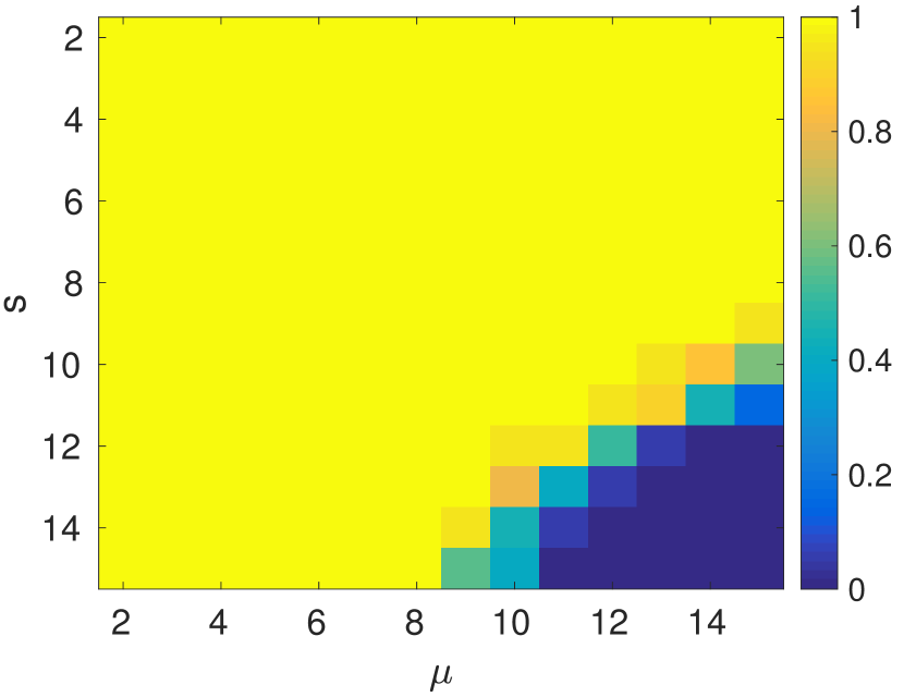
Figure 1: Recovery rate for 2 of 10 active users

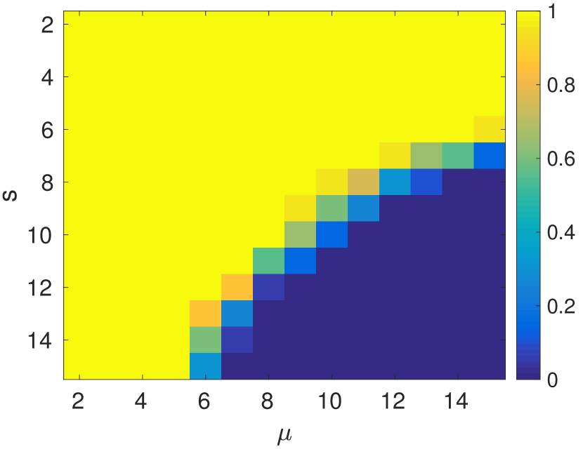
Figure 2: Recovery rate for 3 of 10 active users

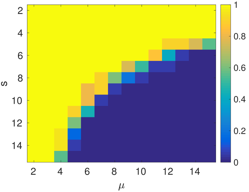
Figure 3: Recovery rate for 4 of 10 active users

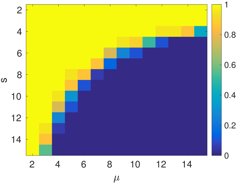
Figure 4: Recovery rate for 5 of 10 active users

VI Conclusions

We have proposed a new access scheme for IoT applications in which many low complexity devices spontaneously send data to a base station in an uncoordinated fashion and included a physical layer security scheme. The base station is able to recover the signals as well as the channels by employing a fast, scalable blind deconvolution algorithm called HiHTP. The benefit of this novel approach is that it requires no pilot signaling to measure the channels, thus greatly reducing the overhead. This is crucial for next generation wireless communication, where the number of devices will increase dramatically. We have provided numerical experiments that show the feasibility of our approach and illustrate the trade-off between the number of active users, the required sparsity of the signals and the channel sparsity. The adaptation of our HiHTP algorithm to the multi-user, multi-antenna case, its robustness to noisy measurements and the proof of rigorous performance guarantees will be a topic of future research.

VII Acknowledgements

We would like to thank the DFG within grants WU 598/7-1, WU 598/8-1, and EI 519/9-1 (DFG Priority Program on Compressed Sensing) and the Templeton Foundation for support. This work has also been performed in the framework of the Horizon 2020 project ONE5G (ICT-760809) receiving funds from the European Union. The authors would like to acknowledge the contributions of their colleagues in the project, although the views expressed in this contribution are those of the authors and do not necessarily represent the project.

References

- [1] M. Shafi, A. F. Molisch, P. J. Smith, T. Haustein, P. Zhu, P. D. Silva, F. Tufvesson, A. Benjebbour, and G. Wunder, “5g: A tutorial overview of standards, trials, challenges, deployment, and practice,” IEEE Journal on Selected Areas in Communications, vol. 35, no. 6, pp. 1201–1221, June 2017.
- [2] G. Wunder, H. Boche, T. Strohmer, and P. Jung, “Sparse Signal Processing Concepts for Efficient 5G System Design,” IEEE ACCESS, December 2015, to appear. [Online]. Available: http://arxiv.org/abs/1411.0435
- [3] G. Wunder, I. Roth, R. Fritschek, and J. Eisert, “HiHTP: A custom-tailored hierarchical sparse detector for massive MTC,” in 49th Annual Asilomar Conf. on Signals, Systems, Pacific Grove, USA, November 2015, November 2017.
- [4] I. Roth, M. Kliesch, G. Wunder, J. Eisert, “Reliable recovery of hierarchically sparse signals and application in machine-type communications,” IEEE Trans. on Signal Processing, May 2017, in revision. [Online]. Available: https://arxiv.org/abs/1612.07806v2
- [5] G. Wunder, C. Stefanovic, and P. Popovski, “Compressive coded random access for massive MTC traffic in 5G systems,” in 49th Annual Asilomar Conf. on Signals, Systems, Pacific Grove, USA, November 2015, November 2015, invited paper.
- [6] G. Wunder, P. Jung, and M. Ramadan, “Compressive random access using a common overloaded control channel,” ArXiv e-prints, appeared at IEEE GLOBECOM’15 (San Diego (USA, December 2015), April 2015. [Online]. Available: https://arxiv.org/abs/1504.05318
- [7] C. T. Zenger and M.-J. Chur and J.-F. Posielek and G. Wunder and C. Paar, “A novel key generating architecture for wireless low-resource devices,” in International Workshop on Secure Internet of Things (SIoT 2014). Wroclaw, Poland: Springer Lecture Notes in Computer Science (LNCS) series, September 2014.
- [8] D. Vasisht, S. Kumar, and D. Katabi, “Decimeter-level localization with a single wifi access point,” in NSDI, 2016, pp. 165–178.
- [9] R. Wilson, D. Tse, and R. A. Scholtz, “Channel identification: Secret sharing using reciprocity in ultrawideband channels,” IEEE Transactions on Information Forensics and Security, vol. 2, no. 3, pp. 364–375, Sept 2007.
- [10] E. J. Candès, T. Strohmer, and V. Voroninski, “PhaseLift: Exact and stable signal recovery from magnitude measurements via convex programming,” Communications on Pure and Applied Mathematics, vol. 66, no. 8, pp. 1241–1274, 2013.
- [11] E. J. Candès, Y. C. Eldar, T. Strohmer, and V. Voroninski, “Phase retrieval via matrix completion,” SIAM J. Imag. Sc., vol. 6, no. 1, pp. 199–225, 2013. [Online]. Available: http://epubs.siam.org/doi/abs/10.1137/110848074
- [12] A. Ahmed, B. Recht, and J. Romberg, “Blind Deconvolution Using Convex Programming,” IEEE Transactions on Information Theory, vol. 60, no. 3, pp. 1711–1732, 2014.
- [13] S. Ling and T. Strohmer, “Blind deconvolution meets blind demixing: Algorithms and performance bounds,” arXiv preprint arXiv:1512.07730, 2015. [Online]. Available: http://arxiv.org/abs/1512.07730
- [14] P. Jung, F. Krahmer, and D. Stöger, “Blind Demixing and Deconvolution at Near-Optimal Rate,” arXiv:1704.04178 [cs, math], Apr. 2017, arXiv: 1704.04178. [Online]. Available: http://arxiv.org/abs/1704.04178
- [15] S. Oymak, A. Jalali, M. Fazel, Y. C. Eldar, and B. Hassibi, “Simultaneously Structured Models With Application to Sparse and Low-Rank Matrices,” IEEE Transactions on Information Theory, vol. 61, no. 5, pp. 2886–2908, May 2015.
- [16] K.-C. Toh, M. J. Todd, and R. H. Tütüncü, “Sdpt3—a matlab software package for semidefinite programming, version 1.3,” Optimization methods and software, vol. 11, no. 1-4, pp. 545–581, 1999.
- [17] J. F. Sturm, “Using sedumi 1.02, a matlab toolbox for optimization over symmetric cones,” Optimization methods and software, vol. 11, no. 1-4, pp. 625–653, 1999.
- [18] A. Flinth, “Sparse Blind Deconvolution and Demixing Through 1 , 2 -Minimization ,” 2017.
- [19] X. Li, S. Ling, T. Strohmer, and K. Wei, “Rapid, robust, and reliable blind deconvolution via nonconvex optimization,” pp. 1–49, 2016. [Online]. Available: http://arxiv.org/abs/1606.04933
- [20] S. Ling and T. Strohmer, “Regularized Gradient Descent: A Nonconvex Recipe for Fast Joint Blind Deconvolution and Demixing,” pp. 1–38, 2017.
- [21] K. Lee, Y. Li, M. Junge, and Y. Bresler, “Stability in blind deconvolution of sparse signals and reconstruction by alternating minimization,” in 2015 International Conference on Sampling Theory and Applications (SampTA), May 2015, pp. 158–162.