Learning the Reward Function for a Misspecified Model

Abstract

In model-based reinforcement learning it is typical to decouple the problems of learning the dynamics model and learning the reward function. However, when the dynamics model is flawed, it may generate erroneous states that would never occur in the true environment. It is not clear a priori what value the reward function should assign to such states. This paper presents a novel error bound that accounts for the reward model’s behavior in states sampled from the model. This bound is used to extend the existing Hallucinated DAgger-MC algorithm, which offers theoretical performance guarantees in deterministic MDPs that do not assume a perfect model can be learned. Empirically, this approach to reward learning can yield dramatic improvements in control performance when the dynamics model is flawed.

,

1 Introduction

In the reinforcement learning problem, an agent interacts with an environment, receiving rewards along the way that indicate the quality of its decisions. The agent’s task is to learn to behave in a way that maximizes reward. Model-based reinforcement learning (MBRL) techniques approach this problem by learning a predictive model of the environment and applying a planning algorithm to the model to make decisions. Intuitively and theoretically (Szita & Szepesvári, 2010), there are many advantages to learning a model of the environment, but MBRL is challenging in practice, since even seemingly minor flaws in the model or the planner can result in catastrophic failure. As a result, model-based methods have generally not been successful in large-scale problems, with only a few notable exceptions (e.g. Abbeel et al., 2007).

This paper addresses an important but understudied problem in MBRL: learning a reward function. It is common for work in model learning to ignore the reward function (e.g. Bellemare et al., 2014; Oh et al., 2015; Chiappa et al., 2017) or, if the model will be used for planning, to assume the reward function is given (e.g. Ross & Bagnell, 2012; Talvitie, 2017; Ebert et al., 2017). Indeed, it is true that if an accurate model of the environment’s dynamics can be learned, reward learning is relatively straightforward – the two problems can be productively decoupled. However, in this paper we will see that when the model class is misspecified (i.e. that the representation does not admit a perfectly accurate model), as is inevitable in problems of genuine interest, the two learning problems are inherently entangled.

1.1 An Example

To better understand how the limitations of the dynamics model impact reward learning, consider Shooter, a simplified video game example introduced by Talvitie (2015), pictured in Figure 1. At the bottom of the screen is a spaceship which can move left and right and fire bullets, which fly upward. When the ship fires a bullet the agent receives -1 reward. Near the top of the screen are three targets. When a bullet hits a target in the middle (bullseye), the target explodes and the agent receives 20 reward; otherwise a hit is worth 10 reward. Figure 1 shows the explosions that indicate how much reward the agent receives.

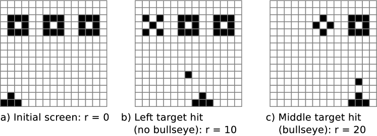
Figure 1: The Shooter domain.

It is typical to decompose the model learning problem into two objectives: dynamics learning and reward learning. In the former the agent must learn to map an input state and action to the next state. In the latter the agent must learn to map a state and action to reward. In this example the agent might learn to associate the presence of explosions with reward. However, this decomposed approach can fail when the dynamics model is imperfect.

For instance, say the dynamics model in this case is a factored MDP, which predicts the value of each pixel in the next image based on the $7\times 5$ neighborhood centered on the pixel. Figure 2b shows a short sample rollout from such a model, sampling each state based on the previous sampled state. The second image in the rollout illustrates the model’s flaw: when predicting the pixel marked with a question mark the model cannot account for the presence of the bullet under the target. Hence, errors appear in the subsequent image (marked with red outlines).

What reward should be associated with this erroneous image? The value the learned model assigns will have a dramatic impact on the extent to which the model is useful for planning and yet it is clear that no amount of traditional data associating environment states with rewards can answer this question. Even a provided, “perfect” reward function would not answer this question; a reward function could assign any value to this state and still be perfectly accurate in states that are reachable in the environment. Intuitively it seems that the best case for planning would be to predict 20 reward for the flawed state, preserving the semantics that a target has been hit in the bullseye. Note, however that this interpretation of the image is specific to this particular flawed model; the reward model’s quality depends on its behavior in states generated by the model rather than the environment.

The remainder of this paper formalizes this intuition. Section 3 presents a novel error bound on value functions in terms of reward error, taking into account the rewards in flawed states generated by the model. In Section 4 the practical implications of this theoretical insight are discussed, leading to an extension of the existing Hallucinated DAgger-MC algorithm, which provides theoretical guarantees in deterministic MDPs, even when the model class is misspecified. Section 5 demonstrates empirically that the approach suggested by the theoretical results can produce good planning performance with a flawed model, while reward models learned in the typical manner (or even “perfect” reward functions) can lead to catastrophic planning failure.

2 Background

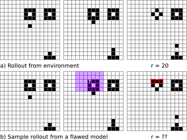
Figure 2: A flawed model may generate states for which the reward function is undefined.

We focus on Markov decision processes (MDP). The environment’s initial state $s_{1}$ is drawn from a distribution $\mu$. At each step $t$ the environment is in a state $s_{t}$. The agent selects an action $a_{t}$ which causes the environment to transition to a new state sampled from the transition distribution: $s_{t+1}\sim P_{s_{t}}^{a_{t}}$. The environment also emits a reward, $R_{s_{t}}^{a_{t}}$. We assume that rewards are bounded within $[0,M]$.

A policy $\pi$ specifies a way to behave in the MDP. Let $\pi(a\mid s)$ be the probability that $\pi$ chooses action $a$ in state $s$. For a sequence of actions $a_{1:t}$ let $P(s^{\prime}\mid s,a_{1:t})=P_{s}^{a_{1:t}}(s^{\prime})$ be the probability of reaching $s^{\prime}$ by starting in $s$ and taking the actions in the sequence. For any state $s$, action $a$, and policy $\pi$, let $D^{t}_{s,a,\pi}$ be the state-action distribution obtained after $t$ steps, starting with state $s$ and action $a$ and thereafter following policy $\pi$. For a state action distribution $\xi$, let $D^{t}_{\xi,\pi}=\operatorname*{{{\mathbf{E}}}}\nolimits_{(s,a)\sim\xi}D^{t}_{s,a,\pi}$. We let $\mathcal{S}$ be the set of states reachable in finite time by some policy with non-zero probability. One may only observe the behavior of $P$ and $R$ in states contained in $\mathcal{S}$.

The $T$-step state-action value of a policy, $Q^{\pi}_{T}(s,a)$ represents the expected discounted sum of rewards obtained by taking action $a$ in state $s$ and executing $\pi$ for an additional $T-1$ steps: $Q^{\pi}_{T}(s,a)=\sum_{t=1}^{T}\gamma^{t-1}\operatorname*{{{\mathbf{E}}}}\nolimits_{(s^{\prime},a^{\prime})\sim D^{t}_{s,a,\pi}}R_{s^{\prime}}^{a^{\prime}}$. Let the $T$-step state value $V^{\pi}_{T}(s)=\operatorname*{{{\mathbf{E}}}}\nolimits_{a\sim\pi_{s}}[Q^{\pi}_{T}(s,a)]$. Let $Q^{\pi}=Q^{\pi}_{\infty}$, and $V^{\pi}=V^{\pi}_{\infty}$. The agent’s goal will be to learn a policy $\pi$ that maximizes $\operatorname*{{{\mathbf{E}}}}\nolimits_{s\sim\mu}[V^{\pi}(s)]$.

In MBRL we seek to learn a dynamics model $\hat{P}$, approximating $P$, and a reward model $\hat{R}$, approximating $R$, and then to use the combined model $(\hat{P},\hat{R})$ to produce a policy via a planning algorithm. We let $\hat{D}$, $\hat{Q}$, and $\hat{V}$ represent the corresponding quantities using the learned model. We assume that $\hat{P}$ and $\hat{R}$ are defined over $\hat{\mathcal{S}}\supseteq\mathcal{S}$; there may be states in $\hat{\mathcal{S}}$ for which $P$ and $R$ are effectively undefined, and it may not be known a priori which states these are.

Let $\mathcal{P}$ represent the dynamics model class, the set of models the learning algorithm could possibly produce and correspondingly let $\mathcal{R}$ be the reward model class. In this work we are most interested in the common case that the dynamics model is misspecified: there is no $\hat{P}\in\mathcal{P}$ that matches $P$ in every $s\in\mathcal{S}$. In this case it is impossible to learn a perfectly accurate model; the agent must make good decisions despite flaws in the learned model. The results in this paper also permit the reward model to be similarly misspecified.

2.1 Bounding Planning Performance

For ease of analysis we focus our attention on the simple one-ply Monte Carlo planning algorithm (one-ply MC), similar to the “rollout algorithm” (Tesauro & Galperin, 1996). For every state-action pair $(s,a)$, the planner executes $N$ $T$-step sample rollouts using $\hat{P}$, starting at $s$, taking action $a$, and then following a rollout policy $\rho$. At each step of the rollout, $\hat{R}$ gives the reward. Let $\bar{Q}(s,a)$ be the average discounted return of the rollouts starting with state $s$ and action $a$. For large $N$, $\bar{Q}$ will closely approximate $\hat{Q}_{T}^{\rho}$ (Kakade, 2003). The execution policy $\hat{\pi}$ will be greedy with respect to $\bar{Q}$. We can place bounds on the quality of $\hat{\pi}$.

For a policy $\pi$ and state-action distribution $\xi$, let $\epsilon_{val}^{\xi,\pi,T}$ be the error in the $T$-step state-action values the model assigns to the policy: $\epsilon_{val}^{\xi,\pi,T}=\operatorname*{{{\mathbf{E}}}}_{(s,a)\sim\xi}\big{[}|Q_{T}^{\pi}(s,a)-\hat{Q}_{T}^{\pi}(s,a)|\big{]}$. For a state distribution $\mu$ and policy $\pi$ let $D_{\mu,\hat{\pi}}(s,a)=\sum_{t=0}^{\infty}\gamma^{t}D_{\mu,\pi}^{t+1}(s,a)$. The following is straightforwardly adapted from an existing bound (Talvitie, 2015, 2017).

Lemma 1.

Let $\bar{Q}$ be the value function returned by applying depth $T$ one-ply Monte Carlo to the model $\hat{P}$ with rollout policy $\rho$. Let $\hat{\pi}$ be greedy w.r.t. $\bar{Q}$. For any policy $\pi$ and state-distribution $\mu$,

$$\operatorname*{{{\mathbf{E}}}}_{s\sim\mu}\big{[}V^{\pi}(s)-V^{\hat{\pi}}(s)\big{]}\leq\frac{4}{1-\gamma}\epsilon_{val}^{\xi,\rho,T}+\epsilon_{mc},$$

where $\xi(s,a)=\frac{1}{2}D_{\mu,\hat{\pi}}(s,a)+\frac{1}{4}D_{\mu,\pi}(s,a)+\frac{1}{4}\left((1-\gamma)\mu(s)\hat{\pi}_{s}(a)+\gamma\sum_{z,b}D_{\mu,\pi}(z,b)P_{z}^{b}(s)\hat{\pi}_{s}(a)\right)$ and $\epsilon_{mc}=\frac{4}{1-\gamma}\|\bar{Q}-\hat{Q}^{\rho}_{T}\|_{\infty}+\frac{2}{1-\gamma}\|BV^{\rho}_{T}-V^{\rho}_{T}\|_{\infty}$ (here $B$ is the Bellman operator).

The $\epsilon_{mc}$ term captures error due to properties of the one-ply MC algorithm: error in the sample average $\bar{Q}$ and the sub-optimality of the $T$-step value function with respect to $\rho$. The $\epsilon_{val}^{\xi,\rho,T}$ term captures error due to the model. The model’s usefulness for planning is tied to the accuracy of the value it assigns to the rollout policy. Thus, in order to obtain a good plan $\hat{\pi}$, we aim to minimize $\epsilon_{val}^{\xi,\rho,T}$.

2.2 Error in the Dynamics Model

If the reward function is known, a bound on $\epsilon_{val}^{\xi,\rho,T}$ in terms of the one-step prediction error of the dynamics model can be adapted from the work of Ross & Bagnell (2012) .

Lemma 2.

For any policy $\pi$ and state-action distribution $\xi$,

$$\epsilon_{val}^{\xi,\pi,T}\leq\frac{M}{1-\gamma}\sum_{t=1}^{T-1}(\gamma^{t}-\gamma^{T})\operatorname*{{{\mathbf{E}}}}_{(s,a)\sim D^{t}_{\xi,\pi}}\big{[}\|P_{s}^{a}-\hat{P}_{s}^{a}\|_{1}\big{]}.$$

Combining Lemmas 1 and 2 yields an overall bound on control performance in terms of model error. However, recent work (Talvitie, 2017) offers a tighter bound in a special case. Let the true dynamics $P$ be deterministic, and let the rollout policy $\rho$ be blind (Bowling et al., 2006); the action selected by $\rho$ is conditionally independent of the current state, given the history of actions. Then for any state-action distribution $\xi$, let $H^{t}_{\xi,\rho}$ be the joint distribution over environment state, model state, and action if a single action sequence is sampled from $\rho$ and then executed in both the model and the environment. So, $H^{1}_{\xi,\rho}(s_{1},z_{1},a_{1})=\xi(s_{1},a_{1})\text{ when }z_{1}=s_{1}\text{ (0 otherwise)}$ and for all $t\geq 2$,

$$H {}^{t}_{\xi,\rho}(s_{t},z_{t},a_{t})=$$

$$\operatorname*{{{\mathbf{E}}}}_{(s_{1},a_{1})\sim\xi}\big{[}\textstyle\sum_{a_{2:t-1}}\rho(a_{2:t}\mid a_{1})P_{s_{1}}^{a_{1:t-1}}(s_{t})\hat{P}_{s_{1}}^{a_{1:t-1}}(z_{t})\big{]}.$$

Since $P$ is deterministic, let $\sigma_{s}^{a_{1:t}}$ be the unique state that results from starting in state $s$ and taking the action sequence $a_{1:t}$. Then Talvitie (2017) offers the following result:

Theorem 3.

If $P$ is deterministic, then for any blind policy $\rho$ and any state-action distribution $\xi$,

$$\epsilon {}_{val}^{\xi,\rho,T}\leq\ M\sum_{t=1}^{T}\gamma^{t-1}\operatorname*{{{\mathbf{E}}}}_{(s,a)\sim\xi}\big{[}\|D^{t}_{s,a,\rho}-\hat{D}^{t}_{s,a,\rho}\|_{1}\big{]}$$ (1)

$$\leq 2M\sum_{t=1}^{T-1}\gamma^{t}\operatorname*{{{\mathbf{E}}}}_{(s,z,a)\sim H^{t}_{\xi,\rho}}\big{[}1-\hat{P}_{z}^{a}(\sigma^{a}_{s})\big{]}$$ (2)

$$\leq\frac{2M}{1-\gamma}\sum_{t=1}^{T-1}(\gamma^{t}-\gamma^{T})\operatorname*{{{\mathbf{E}}}}_{(s,a)\sim D^{t}_{\xi,\rho}}\big{[}1-\hat{P}_{s}^{a}(\sigma^{a}_{s})\big{]}.$$ (3)

Inequality 3 is Lemma 2 in the deterministic case, the bound in terms of the one-step prediction error of $\hat{P}$. Inequality 1 gives the bound in terms of the error in the discounted distribution of states along $T$-step rollouts. Though this is the tightest bound of the three, in practice it is difficult to optimize this objective directly. Inequality 2 gives the bound in terms of hallucinated one-step error, so called because it considers the accuracy of the model’s predictions based on states generated from its own sample rollouts ($z$), rather than states generated by the environment ($s$).

To optimize hallucinated error, the model can be rolled out in parallel with the environment, and trained to predict the next environment state from each “hallucinated” state in the model rollout. Talvitie (2017) shows that this approach can dramatically improve planning performance when the model class is mispecified. Similar approaches have also had empirical success in MBRL tasks (Talvitie, 2014; Venkatraman et al., 2016) and sequence prediction tasks (Venkatraman et al., 2015; Oh et al., 2015; Bengio et al., 2015).

Talvitie (2017) shows that the relative tightness of the hallucinated error bound does not hold for general stochastic dynamics or for arbitrary rollout policies. However, note that these assumptions are not as limiting as they first appear. By far the most common rollout policy chooses actions uniformly randomly, and is thus blind. Furthermore, though $P$ is assumed to be deterministic, it is also assumed to be too complex to be practically captured by $\hat{P}$. From the agent’s perspective, un-modeled complexity will manifest as apparent stochasticity. For example Oh et al. (2015) learned dynamics models of Atari 2600 games, which are fully deterministic (Hausknecht et al., 2014); human players often perceive them to be stochastic due to their complexity. For the remainder of the paper we focus on the special case of deterministic dynamics and blind rollout policies.

3 Incorporating Reward Error

As suggested by Talvitie (2017), there is a straightforward extension of Theorem 3 to account for reward error.

Theorem 4.

If $P$ is deterministic, then for any blind policy $\rho$ and any state-action distribution $\xi$,

$$\epsilon_{val}^{\xi,\rho,T} \leq\sum_{t=1}^{T}\gamma^{t-1}\operatorname*{{{\mathbf{E}}}}_{(s^{\prime},a^{\prime})\sim D^{t}_{\xi,\rho}}\big{[}\big{|}R_{s^{\prime}}^{a^{\prime}}-\hat{R}_{s^{\prime}}^{a^{\prime}}\big{|}\big{]}$$ (4)

$$\hskip 7.22743pt+M\sum_{t=1}^{T}\gamma^{t-1}\operatorname*{{{\mathbf{E}}}}_{(s,a)\sim\xi}\big{[}\|D^{t}_{s,a,\rho}-\hat{D}^{t}_{s,a,\rho}\|_{1}\big{]}$$

$$\leq\sum_{t=1}^{T}\gamma^{t-1}\operatorname*{{{\mathbf{E}}}}_{(s^{\prime},a^{\prime})\sim D^{t}_{\xi,\rho}}\big{[}\big{|}R_{s^{\prime}}^{a^{\prime}}-\hat{R}_{s^{\prime}}^{a^{\prime}}\big{|}\big{]}$$ (5)

$$\hskip 7.22743pt+2M\sum_{t=1}^{T-1}\gamma^{t}\operatorname*{{{\mathbf{E}}}}_{(s,z,a)\sim H^{t}_{\xi,\rho}}\big{[}1-\hat{P}_{z}^{a}(\sigma^{a}_{s})\big{]}$$

$$\leq\sum_{t=1}^{T}\gamma^{t-1}\operatorname*{{{\mathbf{E}}}}_{(s^{\prime},a^{\prime})\sim D^{t}_{\xi,\rho}}\big{[}\big{|}R_{s^{\prime}}^{a^{\prime}}-\hat{R}_{s^{\prime}}^{a^{\prime}}\big{|}\big{]}$$ (6)

$$\hskip 7.22743pt+\frac{2M}{1-\gamma}\sum_{t=1}^{T-1}(\gamma^{t}-\gamma^{T})\operatorname*{{{\mathbf{E}}}}_{(s,a)\sim D^{t}_{\xi,\rho}}\big{[}1-\hat{P}_{s}^{a}(\sigma^{a}_{s})\big{]}.$$

Proof.

The derivation of inequality 4 is below. The rest follow immediately from Theorem 3.

$$\epsilon_{val}^{\xi,\rho,T}=\operatorname*{{{\mathbf{E}}}}_{(s,a)\sim\xi}\big{[}|Q_{T}^{\rho}(s,a)-\hat{Q}_{T}^{\rho}(s,a)|\big{]}$$

$$=\operatorname*{{{\mathbf{E}}}}_{(s,a)\sim\xi}\Bigg{[}\bigg{|}\sum_{t=1}^{T}\gamma^{t-1}\sum_{(s^{\prime},a^{\prime})}\Big{(}D^{t}_{s,a,\rho}(s^{\prime},a^{\prime})R_{s^{\prime}}^{a^{\prime}}$$

$$\hskip 130.08621pt-\hat{D}^{t}_{s,a,\rho}(s^{\prime},a^{\prime})\hat{R}_{s^{\prime}}^{a^{\prime}}\Big{)}\bigg{|}\Bigg{]}$$

$$=\operatorname*{{{\mathbf{E}}}}_{(s,a)\sim\xi}\Bigg{[}\bigg{|}\sum_{t=1}^{T}\gamma^{t-1}\sum_{(s^{\prime},a^{\prime})}\Big{(}D^{t}_{s,a,\rho}(s^{\prime},a^{\prime})R_{s^{\prime}}^{a^{\prime}}$$

$$\hskip 57.81621pt-D^{t}_{s,a,\rho}(s^{\prime},a^{\prime})\hat{R}_{s^{\prime}}^{a^{\prime}}+D^{t}_{s,a,\rho}(s^{\prime},a^{\prime})\hat{R}_{s^{\prime}}^{a^{\prime}}$$

$$\hskip 130.08621pt-\hat{D}^{t}_{s,a,\rho}(s^{\prime},a^{\prime})\hat{R}_{s^{\prime}}^{a^{\prime}}\Big{)}\bigg{|}\Bigg{]}$$

$$=\operatorname*{{{\mathbf{E}}}}_{(s,a)\sim\xi}\Bigg{[}\bigg{|}\sum_{t=1}^{T}\gamma^{t-1}\sum_{(s^{\prime},a^{\prime})}\Big{(}D^{t}_{s,a,\rho}(s^{\prime},a^{\prime})(R_{s^{\prime}}^{a^{\prime}}-\hat{R}_{s^{\prime}}^{a^{\prime}})$$

$$\hskip 65.04256pt+(D^{t}_{s,a,\rho}(s^{\prime},a^{\prime})-\hat{D}^{t}_{s,a,\rho}(s^{\prime},a^{\prime}))\hat{R}_{s^{\prime}}^{a^{\prime}}\Big{)}\bigg{|}\Bigg{]}$$

$$\leq\sum_{t=1}^{T}\gamma^{t-1}\operatorname*{{{\mathbf{E}}}}_{(s^{\prime},a^{\prime})\sim D^{t}_{\xi,\rho}}\big{|}R_{s^{\prime}}^{a^{\prime}}-\hat{R}_{s^{\prime}}^{a^{\prime}}\big{|}$$

$$\hskip 50.58878pt+M\sum_{t=1}^{T}\gamma^{t-1}\operatorname*{{{\mathbf{E}}}}_{(s,a)\sim\xi}\big{[}\big{\|}D^{t}_{s,a,\rho}-\hat{D}^{t}_{s,a,\rho}\big{\|}\big{]},$$

which gives the result. ∎

As is typical, these bounds break the value error into two parts: reward error and dynamics error. The reward error measures the accuracy of the reward model in environment states encountered by policy $\rho$. The dynamics error measures the probability that the model will generate the correct states in rollouts, effectively assigning maximum reward error ($M$) when the dynamics model generates incorrect states. This view corresponds to common MBRL practice: train the dynamics model to assign high probability to correct environment states and the reward model to accurately map environment states to rewards. However, as discussed in Section 1.1, these bounds are overly conservative (and thus loose): generating an erroneous state need not be catastrophic if the associated reward is still reasonable. We can derive a bound that accounts for this.

Theorem 5.

If $P$ is deterministic, then for any blind policy $\rho$ and any state-action distribution $\xi$,

$$\epsilon_{val}^{\xi,\rho,T} \leq\sum_{t=1}^{T}\gamma^{t-1}\operatorname*{{{\mathbf{E}}}}\nolimits_{(s,z,a)\sim H^{t}_{\xi,\rho}}\big{[}\big{|}R_{s}^{a}-\hat{R}_{z}^{a}\big{|}\big{]}.$$

Proof.

$$\epsilon_{val}^{\xi,\rho,T}=\operatorname*{{{\mathbf{E}}}}\nolimits_{(s_{1},a_{1})\sim\xi}\big{[}\big{|}Q_{\rho}^{T}(s_{1},a_{1})-\hat{Q}_{\rho}^{T}(s_{1},a_{1})\big{|}\big{]}$$

$$=\operatorname*{{{\mathbf{E}}}}_{(s_{1},a_{1})\sim\xi}\Bigg{[}\Bigg{|}\sum_{t=1}^{T}\gamma^{t-1}\sum_{s_{t},a_{t}}D^{t}_{s_{1},a_{1},\rho}(s_{t},a_{t})R_{s_{t}}^{a_{t}}$$

$$\hskip 115.63243pt-\sum_{z_{t},a_{t}}\hat{D}^{t}_{s_{1},a_{1},\rho}(z_{t},a_{t})\hat{R}_{z_{t}}^{a_{t}}\Bigg{|}\Bigg{]}$$

$$=\operatorname*{{{\mathbf{E}}}}_{(s_{1},a_{1})\sim\xi}\Bigg{[}\Bigg{|}\big{(}R_{s_{1}}^{a_{1}}-\hat{R}_{s_{1}}^{a_{1}}\big{)}+\sum_{t=2}^{T}\gamma^{t-1}\sum_{a_{2:t}}\rho(a_{2:t}\mid a_{1})$$

$$\hskip 36.135pt\bigg{(}\sum_{s_{t}}P_{s_{1}}^{a_{1:t-1}}(s_{t})R_{s_{t}}^{a_{t}}-\sum_{z_{t}}\hat{P}_{s_{1}}^{a_{1:t-1}}(z_{t})\hat{R}_{z_{t}}^{a_{t}}\bigg{)}\Bigg{|}\Bigg{]}.$$

Now note that for $t\geq 2$,

$$\sum_{s_{t}}P_{s_{1}}^{a_{1:t-1}}(s_{t})R_{s_{t}}^{a_{t}}-\sum_{z_{t}}\hat{P}_{s_{1}}^{a_{1:t-1}}(z_{t})\hat{R}_{z_{t}}^{a_{t}}$$

$$=\sum_{s_{t}}P_{s_{1}}^{a_{1:t-1}}(s_{t})R_{s_{t}}^{a_{t}}\sum_{z_{t}}\hat{P}_{s_{1}}^{a_{1:t-1}}(z_{t})$$

$$\hskip 79.49744pt-\sum_{z_{t}}\hat{P}_{s_{1}}^{a_{1:t-1}}(z_{t})\hat{R}_{z_{t}}^{a_{t}}\sum_{s_{t}}P_{s_{1}}^{a_{1:t-1}}(s_{t})$$

$$=\sum_{s_{t},z_{t}}P_{s_{1}}^{a_{1:t-1}}(s_{t})\hat{P}_{s_{1}}^{a_{1:t-1}}(z_{t})\big{(}R_{s_{t}}^{a_{t}}-\hat{R}_{z_{t}}^{a_{t}}\big{)}$$

Thus

$$\epsilon_{val}^{\xi,\rho,T}\leq\operatorname*{{{\mathbf{E}}}}_{(s_{1},a_{1})\sim\xi}\Bigg{[}\big{|}R_{s_{1}}^{a_{1}}-\hat{R}_{s_{1}}^{a_{1}}\big{|}+\sum_{t=2}^{T}\gamma^{t-1}$$

$$\sum_{a_{2:t}}\rho(a_{2:t}\mid a_{1})\sum_{s_{t},z_{t}}P_{s_{1}}^{a_{1:t-1}}(s_{t})\hat{P}_{s_{1}}^{a_{1:t-1}}(z_{t})\big{|}R_{s_{t}}^{a_{t}}-\hat{R}_{z_{t}}^{a_{t}}\big{|}\Bigg{]}$$

$$=\sum_{t=1}^{T}\gamma^{t-1}\operatorname*{{{\mathbf{E}}}}_{(s,z,a)\sim H^{t}_{\xi,\rho}}\big{[}\big{|}R_{s}^{a}-\hat{R}_{z}^{a}\big{|}\big{]}.$$

Similar to the hallucinated one-step error for the dynamics model (inequality 2), Theorem 5 imagines that the model and the environment are rolled out in parallel. It measures the error between the rewards generated in the model rollout and the rewards in the corresponding steps of the environment rollout. We call this the hallucinated reward error. However, unlike the bounds in Theorem 4, which are focused on the model placing high probability on “correct” states, the hallucinated reward error may be small even if the state sequence sampled from the dynamics model is “incorrect”, as long as the sequence of rewards is similar. As such, we can show that this bound is tighter than inequality 5 and thus more closely related to planning performance.

Theorem 6.

If $P$ is deterministic, then for any blind policy $\rho$ and any state-action distribution $\xi$,

$$\sum_{t=1}^{T} \gamma^{t-1}\operatorname*{{{\mathbf{E}}}}\nolimits_{(s,z,a)\sim H^{t}_{\xi,\rho}}\big{[}\big{|}R_{s}^{a}-\hat{R}_{z}^{a}\big{|}\big{]}$$

$$\leq\sum_{t=1}^{T}\gamma^{t-1}\operatorname*{{{\mathbf{E}}}}_{(s^{\prime},a^{\prime})\sim D^{t}_{\xi,\rho}}\big{[}\big{|}R_{s^{\prime}}^{a^{\prime}}-\hat{R}_{s^{\prime}}^{a^{\prime}}\big{|}\big{]}$$

$$\hskip 43.36243pt+2M\sum_{t=1}^{T-1}\gamma^{t}\operatorname*{{{\mathbf{E}}}}_{(s,z,a)\sim H^{t}_{\xi,\rho}}\big{[}1-\hat{P}_{z}^{a}(\sigma^{a}_{s})\big{]}.$$

Proof.

$$\sum_{t=1}^{T} \gamma^{t-1}\operatorname*{{{\mathbf{E}}}}_{(s,z,a)\sim H^{t}_{\xi,\rho}}\big{[}\big{|}R(s,a)-\hat{R}(z,a)\big{|}\big{]}$$

$$=\sum_{t=1}^{T}\gamma^{t-1}\sum_{s,z,a}H^{t}_{\xi,\rho}(s,z,a)\big{|}R(s,a)-\hat{R}(z,a)\big{|}$$

$$=\sum_{t=1}^{T}\gamma^{t-1}\sum_{s,a}H^{t}_{\xi,\rho}(s,s,a)\big{|}R(s,a)-\hat{R}(s,a)\big{|}$$

$$\hskip 7.22743pt+\sum_{t=1}^{T}\gamma^{t-1}\sum_{s,z\neq s,a}H^{t}_{\xi,\rho}(s,z,a)\big{|}R(s,a)-\hat{R}(z,a)\big{|}.$$

This breaks the expression into two terms. Now consider the first term:

$$\sum_{t=1}^{T} \gamma^{t-1}\sum_{s,a}H^{t}_{\xi,\rho}(s,s,a)\big{|}R(s,a)-\hat{R}(s,a)\big{|}$$

$$\leq\sum_{t=1}^{T}\gamma^{t-1}\sum_{s,a}D^{t}_{\xi,\rho}(s,a)\big{|}R(s,a)-\hat{R}(s,a)\big{|}.$$ (7)

Now consider the second term:

$$\sum_{t=1}^{T} \gamma^{t-1}\sum_{s,z\neq s,a}H^{t}_{\xi,\rho}(s,z,a)\big{|}R(s,a)-\hat{R}(z,a)\big{|}$$

$$\leq M\sum_{t=1}^{T}\gamma^{t-1}\sum_{s,z\neq s,a}H^{t}_{\xi,\rho}(s,z,a).$$

Recall that $H^{1}_{\xi,\rho}(s,z,a)=0$ if $s\neq z$. Thus,

$$M\sum_{t=1}^{T}\gamma^{t-1}\sum_{s,z\neq s,a}H^{t}_{\xi,\rho}(s,z,a)$$

$$=M\sum_{t=1}^{T-1}\gamma^{t}\sum_{s,z\neq s,a}H^{t+1}_{\xi,\rho}(s,z,a)$$

$$=M\sum_{s^{\prime},z^{\prime},a^{\prime}}\Bigg{(}\sum_{s,z\neq s}P^{a^{\prime}}_{s^{\prime}}(s)\hat{P}^{a^{\prime}}_{z^{\prime}}(z)\Bigg{)}\sum_{t=1}^{T-1}\gamma^{t}H^{t}_{\xi,\rho}(s^{\prime},z^{\prime},a^{\prime})$$

$$=M\sum_{s^{\prime},z^{\prime},a^{\prime}}\big{(}1-\hat{P}^{a^{\prime}}_{z^{\prime}}(\sigma^{a^{\prime}}_{s^{\prime}})\big{)}\sum_{t=1}^{T-1}\gamma^{t}H^{t}_{\xi,\rho}(s^{\prime},z^{\prime},a^{\prime})$$

$$=M\sum_{t=1}^{T-1}\gamma^{t}\operatorname*{{{\mathbf{E}}}}_{(s,z,a)\sim H^{t}_{\xi,\rho}}[1-\hat{P}^{a}_{z}(\sigma^{a}_{s})].$$ (8)

Combining lines 7 and 8 yields the result. ∎

The next section discusses the practical and conceptual implications of this result for MBRL algorithms and extends an existing MBRL algorithm to incorporate this insight.

4 Implications for MBRL

This is not the first observation that the reward model should be specialized to the dynamics model . Sorg et al. (2010b) argued as we have that when the model or planner are limited in some way, reward functions other than the true reward may lead to better planning performance. Accordingly, policy gradient approaches have been employed to learn reward functions for use with online planning algorithms, providing a benefit even when the reward function is known (Sorg et al., 2010a, 2011; Bratman et al., 2012; Guo et al., 2016). Tamar et al. (2016) take this idea to its logical extreme, treating the entire model and even the planning algorithm itself as a policy parameterization, adapting them to directly improve control performance rather than to minimize any measure of prediction error. Though appealing in its directness, this approach offers little theoretical insight into what makes a model useful for planning. Furthermore, there are advantages to optimizing quantities other than control performance; this allows the model to exploit incoming data even when it is unclear how to improve the agent’s policy (for instance if the agent has seen little reward). Theorem 5 provides more specific guidance about how to choose amongst a set of flawed models. Rather than attempting to directly optimize control performance, this result suggests that we can take advantage of reward error signals while still offering guarantees in terms of control performance.

It is notable that, unlike Theorem 4, Theorem 5 does not contain a term measuring dynamics error. Certainly the dynamics model is implicitly important; for some choices of $\hat{P}$ the hallucinated reward error can be made very small while for others it may be irreducibly high (for instance if $\hat{P}$ simply loops on a single state). Nevertheless, low hallucinated reward error does not require that the dynamics model place high probability on “correct” states. In fact, it may be that dynamics entirely unrelated to the environment yield the best reward predictions. This intriguingly suggests that the dynamics model and reward model parameters could be adapted together to optimize hallucinated reward error. Arguably, the recently introduced Predictrons (Silver et al., 2017) and Value Prediction Networks (Oh et al., 2017) are attempts to do just this – they adapt the model’s dynamics solely to improve reward prediction. We can see Theorem 5 as theoretical support for these approaches and encouragement of more study in this direction. Still, in practice it may be much harder to learn to predict reward sequences than state sequences, especially when the reward signal is sparse. Also, the relationship between reward prediction error and dynamics model parameters can be highly complex, which may make theoretical performance guarantees difficult.

Another possible interpretation of Theorem 5 is that the reward model should be customized to the dynamics model. That is, if we hold the dynamics model fixed, then the result gives a clear objective for the reward model. Theorem 6 suggests an algorithmic structure where the dynamics model is trained via its own objective, and the reward model is then trained to minimize hallucinated error with respect to the learned dynamics model. The clear downside of this approach is that it will not in general find the best combination of dynamics model and reward model; it could be that a less accurate dynamics model results in lower hallucinated reward error. The advantage is that it allows us to effectively exploit the prediction error signal for the dynamics model and removes the circular dependence between the dynamics model and the reward model.

In this paper we explore this avenue by extending the existing Hallucinated DAgger-MC algorithm (Talvitie, 2017). Because the resulting algorithm is very similar to the original, we leave a detailed description and analysis to the appendix and here focus on key, high-level points. Section 5 presents empirical results illustrating the practical impact of training the reward model to minimize hallucinated error.

4.1 Hallucinated DAgger-MC with Reward Learning

The “Data Aggregator” (DAgger) algorithm (Ross & Bagnell, 2012) was the first practically implementable MBRL algorithm with performance guarantees agnostic to the model class. It did, however, require that the planner be near optimal. DAgger-MC (Talvitie, 2015) relaxed this assumption, accounting for the limitations of a particular suboptimal planner (one-ply MC). Hallucinated DAgger-MC (or H-DAgger-MC) (Talvitie, 2017) altered DAgger-MC to optimize the hallucinated error, rather than the one-step error. All of these algorithms were presented under the assumption that the reward function was known a priori. As we will see in Section 5, the reward function cannot be ignored; even when the reward function is given, these algorithms can fail catastrophically due to the interaction between the reward function and small errors in the dynamics model.

At a high level, H-DAgger-MC proceeds in iterations. In each iteration a batch of data is gathered by sampling state-action pairs using a mixture of the current plan and an “exploration distribution” (to ensure that important states are visited, even if the plan would not visit them). The rollout policy is used to generate parallel rollouts in the environment and model from these sampled state-action pairs, which form the training examples (with model state as input and environment state as output). The collected data is used to update the dynamics model, which is then used to produce a new plan to be used in the next iteration. We simply augment H-DAgger-MC, adding a reward learning step to each iteration (rather than assuming the reward is given). In each rollout, training examples mapping “hallucinated” model states to the real environment rewards are collected and used to update the reward model.

The extended H-DAgger-MC algorithm offers theoretical guarantees similar to those of the original algorithm. Essentially, if

• the exploration distribution is similar to the state visitation distribution of a good policy,

• $\epsilon_{mc}$ is small,

• the learning algorithms for the dynamics model and reward model are both no-regret, and

• the reward model class $\mathcal{R}$ contains a low hallucinated reward error model with respect to the lowest hallucinated prediction error model in $\mathcal{P}$,

then in the limit H-DAgger-MC will produce a good policy. As discussed in Section 4, this does not guarantee that H-DAgger-MC will find the best performing combination of dynamics model and reward model, since the training of the dynamics model does not take hallucinated reward error into account. It is, however, an improvement over the original H-DAgger-MC result in that good performance can be assured even if there is no low error dynamics model in $\mathcal{P}$, as long as there is a low error reward model in $\mathcal{R}$.

For completeness’ sake, a more detailed description and analysis of the algorithm can be found in the appendix. Here we turn to an empirical evaluation of the algorithm.

5 Experiments

In this section we illustrate the impact of optimizing hallucinated reward error in the Shooter example described in Section 1 using both DAgger-MC and H-DAgger-MC. The one-ply MC planner used 50 uniformly random rollouts of depth 20 per action at every step. The exploration distribution was generated by following the optimal policy with $(1-\gamma)$ probability of termination at each step. The discount factor was $\gamma=0.9$. In each iteration 500 training rollouts were generated and the resulting policy was evaluated in an episode of length 30. The discounted return obtained by the policy in each iteration is reported, averaged over 50 trials.

The dynamics model for each pixel was learned using Context Tree Switching (Veness et al., 2012), similar to the FAC-CTW algorithm (Veness et al., 2011). At each position the model takes as input the values of the pixels in a $w\times h$ neighborhood around the position in the previous timestep. Data was shared across all positions. The reward was approximated with a linear function for each action, learned via stochastic weighted gradient descent. The feature representation contained a binary feature for each possible $3\times 3$ configuration of pixels at each position. This representation admits a perfectly accurate reward model. The qualitative observations presented in this section were robust to a wide range of choices of step size for gradient descent. Here, in each experiment the best performing step size for each approach is selected from 0.005, 0.01, 0.05, 0.1, and 0.5.

In the experiments a practical alteration has been made to the H-DAgger-MC algorithm. H-DAgger-MC requires an “unrolled” dynamics model (with a separate model for each step of the rollout, each making predictions based on the output of the previous model). While this is important for H-DAgger-MC’s theoretical guarantees, Talvitie (2017) found empirically that a single dynamics model for all steps could be learned, provided that the training rollouts had limited depth. Following Talvitie (2017), in the first 10 iterations only the first example from each training rollout is added to the dynamics model dataset; thereafter only the first two examples are added. The entire rollout was used to train the reward model. DAgger-MC does not require an unrolled dynamics model or truncated training rollouts and was implemented as originally presented, with a single dynamics model and full training rollouts (Talvitie, 2015).

5.1 Results

We consider both DAgger-MC and H-DAgger-MC with a perfect reward model, a reward model trained only on environment states during rollouts, and a reward model trained on “hallucinated” states as described in Section 4.1. The perfect reward model is one that someone familiar with the rules of the game would likely specify; it simply checks for the presence of explosions in the three target positions and gives the appropriate value if an explosion is present or 0 otherwise (subtracting 1 if the action is “shoot”). Results are presented in three variations on the Shooter problem.

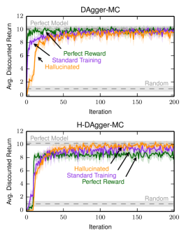
(a) No model limitations

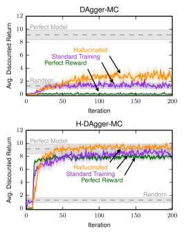
(b) Moving bullseyes (2nd-order Markov)

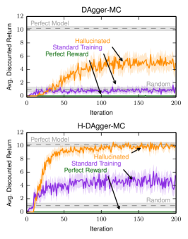
(c) Pixel models use $5\times 7$ neighborhood

Figure 3: Performance of DAgger-MC and H-DAgger-MC in three variations on the Shooter domain.

5.1.1 No Model Limitations

In the first experiment we apply these algorithms to Shooter, as described in Section 1. Here, the dynamics model uses a $7\times 7$ neighborhood, which is sufficient to make perfectly accurate predictions for every pixel. Figure 3a shows the discounted return of the policies generated by DAgger-MC and H-DAgger-MC, averaged over 50 independent trials. The shaded region surrounding each curve represents a 95% confidence interval. The gray line marked “Random” shows the average discounted return of the uniform random policy (with a 95% confidence interval). The gray line marked “Perfect Model” shows the average discounted return of the one-ply MC planner using a perfect model.

Unsurprisingly, the performance DAgger-MC is comparable to that of planning with the perfect model. As observed by Talvitie (2017), with the perfect reward model H-DAgger-MC performs slightly worse than DAgger-MC; the dynamics model in H-DAgger-MC receives noisier data and is thus less accurate. Interestingly, we can now see that the learned reward model yields better performance than the perfect reward model, even without hallucinated training! The perfect reward model relies on specific screen configurations that are less likely to appear in flawed sample rollouts, but the learned reward model generalizes to screens not seen during training. Of course, it is coincidental that this generalization is beneficial; under standard training the reward model is only trained in environment states, giving no guidance in erroneous model states. Hallucinated training specifically trains the reward model to make reasonable predictions during model rollouts, so it yields better performance, comparable with that of DAgger-MC. Thus we see that learning the reward function in this way mitigates a shortcoming of H-DAgger-MC, making it more effective in practice when a perfectly accurate model can be learned.

5.1.2 Failure of the Markov Assumption

Next we consider a version of shooter presented by Talvitie (2017) in which the bullseye in each target moves from side to side, making the environment second-order Markov. Because the model is Markov, it cannot accurately predict the movement of the bullseyes, though the representation is sufficient to accurately predict every other pixel.

Figure 3b shows the results. As Talvitie (2017) observed, DAgger-MC fails catastrophically in this case. Though the model’s limitation only prevents it from accurately predicting the bullseyes, the resulting errors compound during rollouts, quickly rendering them useless. As previously observed, H-DAgger-MC performs much better, as it trains the model to produce more stable rollouts. In both cases we see again that the learned reward models outperform the perfect reward model, and hallucinated reward training yields the best performance, even allowing DAgger-MC to perform better than the random policy.

5.1.3 Flawed Factored Structure

We can see the importance of hallucinated reward training even more clearly when we consider the original Shooter domain (with static bullseyes), but limit the size of the neighborhood used to predict each pixel, as described in Section 1.1. Figure 3c shows the results. Once again DAgger-MC fails. Again we see that the learned reward models yield better performance than the perfect reward function, and that hallucinated training guides the reward model to be useful for planning, despite the flaws in the dynamics model.

In this case, we can see that H-DAgger-MC also fails when combined with the perfect reward model, and performs poorly with the reward model trained only on environment states. Hallucinated training helps the dynamics model produce stable sample rollouts, but does not correct the fundamental limitation: the dynamics model cannot accurately predict the shape of the explosion when a target is hit. As a result, a reward model that bases its predictions only the explosions that occur in the environment will consistently fail to predict reward when the agent hits a target in sample rollouts. Hallucinated training, in contrast, specializes the reward model to the flawed dynamics model, allowing for performance comparable to planning with a perfect model.

6 Conclusion

This paper has introduced hallucinated reward error, which measures the extent to which the rewards in a sample rollout from the model match the rewards in a parallel rollout from the environment. Under some conditions, this quantity is more tightly related to control performance than the more traditional measure of model quality (reward error in environment states plus error in state transition). Empirically we have seen that when the dynamics model is flawed, reward functions learned in the typical manner and even “perfect” reward functions given a priori can lead to catastrophic planning failure. When the reward function is trained to minimize hallucinated reward error, it specifically accounts for the model’s flaws, significantly improving performance.

Appendix A Hallucinated DAgger-MC Details

Hallucinated DAgger-MC, like earlier variations on DAgger, requires the ability to reset to the initial state distribution $\mu$ and also the ability to reset to an “exploration distribution” $\nu$. The exploration distribution ideally ensures that the agent will encounter states that would be visited by a good policy. The performance bound for H-DAgger-MC depends in part on the quality of the selected $\nu$.

In addition to assuming a particular form for the planner (one-ply MC with a blind rollout policy), H-DAgger-MC requires the dynamics model to be “unrolled”. Rather than learning a single $\hat{P}$, H-DAgger-MC learns a set $\{\hat{P}^{1},\ldots,\hat{P}^{T-1}\}\subseteq\mathcal{P}$, where model $\hat{P}^{i}$ is responsible for predicting the outcome of step $i$ of a rollout, given the state sampled from $\hat{P}^{i-1}$. While this impractical condition is important theoretically, Talvitie (2017) showed that in practice a single $\mathcal{P}$ can be used for all steps; the experiments in Section 5 make use of this practical alteration.

Algorithm 1 augments H-DAgger-MC to learn a reward model as well as a dynamics model. In particular, H-DAgger-MC proceeds in iterations, each iteration producing a new plan, which is turn used to collect data to train a new model. In each iteration state-action pairs are sampled using the current plan and the exploration distribution (lines 7-13), and then the world and model are rolled out in parallel to generate hallucinated training examples (lines 14-21). The resulting data is used to update the model. We simply add a reward model learning process, and collect training examples along with the state transition examples during the rollout. After both parts of the model have been updated, a new plan is generated for the subsequent iteration. Note that while the dynamics model is “unrolled”, there is only a single reward model that is responsible for predicting the reward at every step of the rollout. We assume that the reward learning algorithm is performing a weighted regression (where each training example is weighted by $\gamma^{t-1}$ for the rollout step $t$ in which it occurred).

Algorithm 1 Hallucinated DAgger-MC (+ reward learning)

0:  Learn-Dynamics, Learn-Reward, exploration distr. $\nu$, MC-Planner(blind rollout policy $\rho$, depth $T$), # iterations $N$, # rollouts per iteration $K$.

1:  Get initial datasets $\mathcal{D}^{1:T-1}_{1}$ and $\mathcal{E}_{1}$ (maybe using $\nu$)

2:  Initialize $\hat{P}^{1:T-1}_{1}\leftarrow$ Learn-Dynamics($\mathcal{D}^{1:T-1}_{1}$).

3:  Initialize $\hat{R}_{1}\leftarrow$ Learn-Reward($\mathcal{E}_{1}$).

4:  Initialize $\hat{\pi}_{1}\leftarrow$ MC-Planner($\hat{P}^{1:T-1}_{1}$, $\hat{R}_{1}$).

5:  for $n\leftarrow 2\ldots N$ do

6:     for $k\leftarrow 1\ldots K$ do

7:        With probability… $\triangleright$ First sample from $\xi$

8:            $\nicefrac{{1}}{{2}}$: Sample $(x,b)\sim D_{\mu}^{\hat{\pi}_{n}}$

9:            $\nicefrac{{1}}{{4}}$: Reset to $(x,b)\sim\nu$.

10:            $\nicefrac{{(1-\gamma)}}{{4}}$: Sample $x\sim\mu$, $b\sim\hat{\pi}_{n}(\cdot\mid x)$.

11:            $\nicefrac{{\gamma}}{{4}}$: Reset to $(y,c)\sim\nu$

12:                  Sample $x\sim P(\cdot\mid y,c)$, $b\sim\hat{\pi}_{n}(\cdot\mid x)$

13:        Let $s\leftarrow x$, $z\leftarrow x$, $a\leftarrow b$.

14:        for $t\leftarrow 1\ldots T-1$ do $\triangleright$ Parallel rollouts…

15:           Sample $s^{\prime}\sim P(\cdot\mid s,a)$.

16:           Add $\langle z,a,s^{\prime}\rangle$ to $\mathcal{D}^{t}_{n}$. $\triangleright$ (DAgger-MC adds $\langle s,a,s^{\prime}\rangle$)

17:           Add $\langle z,a,R_{s}^{a},\gamma^{t-1}\rangle$ to $\mathcal{E}_{n}$.$\triangleright$ (Standard approach adds $\langle s,a,R_{s}^{a},\gamma^{t-1}\rangle$)

18:           Sample $z^{\prime}\sim\hat{P}^{t}_{n-1}(\cdot\mid z,a)$.

19:           Let $s\leftarrow s^{\prime}$, $z\leftarrow z^{\prime}$, and sample $a\sim\rho$.

20:        end for

21:        Add $\langle z,a,R_{s}^{a},\gamma^{T-1}\rangle$ to $\mathcal{E}_{n}$.$\triangleright$ (Standard approach adds $\langle s,a,R_{s}^{a},\gamma^{T-1}\rangle$)

22:     end for

23:     $\hat{P}^{1:T-1}_{n}\leftarrow$ Learn-Dynamics($\hat{P}^{1:T-1}_{n-1}$, $\mathcal{D}^{1:T-1}_{n}$)

24:     $\hat{R}_{n}\leftarrow$ Learn-Reward($\hat{R}_{n-1}$, $\mathcal{E}_{n}$)

25:     $\hat{\pi}_{n}\leftarrow$ MC-Planner($\hat{P}^{1:T-1}_{n}$, $\hat{R}_{n}$).

26:  end for

27:  return the sequence $\hat{\pi}_{1:N}$

A.1 Analysis of H-DAgger-MC

We now derive theoretical guarantees for this new version of H-DAgger-MC. The analysis is similar to that of existing DAgger variants (Ross & Bagnell, 2012; Talvitie, 2015, 2017), but the proof is included for completeness. Let $H^{t}_{n}$ be the distribution from which H-DAgger-MC samples a training example at depth $t$ (lines 7-13 to pick an initial state-action pair, lines 14-21 to roll out). Define the average error of the dynamics model at depth $t$ to be

$$\bar{\epsilon}^{t}_{prd}=\frac{1}{N}\sum_{n=1}^{N}\operatorname*{{{\mathbf{E}}}}\nolimits_{(s,z,a)\sim H^{t}_{n}}[1-\hat{P}_{n}^{t}(\sigma_{s}^{a}\mid z,a)].$$

Let $\epsilon_{\hat{R}_{n}}(s,z,a)=|R(s,a)-\hat{R}_{n}(z,a)|$ and let

$$\bar{\epsilon}_{hrwd}=\frac{1}{N}\sum_{n=1}^{N}\sum_{t=1}^{T}\gamma^{t-1}\operatorname*{{{\mathbf{E}}}}\nolimits_{(s,z,a)\sim H^{t}_{n}}[\epsilon_{\hat{R}_{n}}(s,z,a)|]$$

be the average reward model error. Finally, let $D^{t}_{n}$ be the distribution from which H-DAgger-MC samples $s$ and $a$ during the rollout in lines 14-21. The error of the reward model with respect to these environment states is

$$\bar{\epsilon}_{erwd}=\frac{1}{N}\sum_{n=1}^{N}\sum_{t=1}^{T}\gamma^{t-1}\operatorname*{{{\mathbf{E}}}}\nolimits_{(s,a)\sim D^{t}_{n}}[|R(s,a)-\hat{R}(s,a)|].$$

For a policy $\pi$, let $c_{\nu}^{\pi}=\sup_{s,a}\frac{D_{\mu,\pi}(s,a)}{\nu(s,a)}$ represent the mismatch between the discounted state-action distribution under $\pi$ and the exploration distribution $\nu$. Now, consider the sequence of policies $\hat{\pi}_{1:N}$ generated by H-DAgger-MC. Let $\bar{\pi}$ be the uniform mixture over all policies in the sequence. Let $\bar{\epsilon}_{mc}=\frac{1}{N}\frac{4}{1-\gamma}\sum_{n=1}^{N}\|\bar{Q}_{n}-\hat{Q}^{\rho}_{T,n}\|_{\infty}+\frac{2}{1-\gamma}\|BV^{\rho}_{T}-V^{\rho}_{T}\|_{\infty}$ be the error induced by the choice of planning algorithm, averaged over all iterations.

Lemma 7.

In H-DAgger-MC, the policies $\hat{\pi}_{1:N}$ are such that for any policy $\pi$,

$$\operatorname*{{{\mathbf{E}}}}_{s\sim\mu} \big{[}V^{\pi}(s)-V^{\bar{\pi}}(s)\big{]}\leq\frac{4}{1-\gamma}c^{\pi}_{\nu}\bar{\epsilon}_{hrwd}+\bar{\epsilon}_{mc}$$

$$\leq\frac{4}{1-\gamma}c^{\pi}_{\nu}\Big{(}\bar{\epsilon}_{erwd}+2M\sum_{t=1}^{T-1}\gamma^{t-1}\bar{\epsilon}^{t}_{prd}\Big{)}+\bar{\epsilon}_{mc}.$$

Proof.

Recall that

$$\operatorname*{{{\mathbf{E}}}}_{s\sim\mu}\big{[}V^{\pi}(s)-V^{\bar{\pi}}(s)\big{]}=\frac{1}{N}\sum_{n=1}^{N}\operatorname*{{{\mathbf{E}}}}_{s\sim\mu}\big{[}V^{\pi}(s)-V^{\hat{\pi}_{n}}(s)\big{]}.$$

and by Lemma 1 for any $n\geq 1$,

$$\operatorname*{{{\mathbf{E}}}}_{s\sim\mu}\big{[}V^{\pi}(s)-V^{\hat{\pi}_{n}}(s)\big{]}\leq$$

$$\hskip 28.90755pt\frac{4}{1-\gamma}\operatorname*{{{\mathbf{E}}}}_{(s,a)\sim\xi^{\pi,\hat{\pi}_{n}}_{\mu}}[|\hat{Q}_{T,n}^{\rho}(s,a)-Q_{T}^{\rho}(s,a)|]+\bar{\epsilon}_{mc},$$

where

$$\xi^{\pi,\hat{\pi}_{n}}_{\mu}(s,a)=\frac{1}{2} D_{\mu,\hat{\pi}_{n}}(s,a)+\frac{1}{4}D_{\mu,\pi}(s,a)$$

$$+\frac{1}{4}\Big{(}(1-\gamma)\mu(s)\hat{\pi}_{n}(a\mid s)$$

$$\hskip 7.22743pt+\gamma\sum_{z,b}D_{\mu,\pi}(z,b)P_{z}^{b}(s)\hat{\pi}_{n}(a\mid s)\Big{)}.$$

Then, combining the above with Theorem 5,

$$\frac{1}{N}\sum_{n=1}^{N}\frac{4}{1-\gamma}\operatorname*{{{\mathbf{E}}}}_{(s,a)\sim\xi^{\pi,\hat{\pi}_{n}}_{\mu}}[|\hat{Q}_{T,n}^{\rho}(s,a)-Q_{T}^{\rho}(s,a)|]+\bar{\epsilon}_{mc}$$

$$\leq\frac{1}{N}\sum_{n=1}^{N}\frac{4}{1-\gamma}\sum_{t=1}^{T}\gamma^{t-1}\operatorname*{{{\mathbf{E}}}}_{\scriptsize\begin{aligned} &(s,z,a)\\ &\sim H^{t,n}_{\xi_{\mu}^{\pi,\hat{\pi}_{n}},\rho}\end{aligned}}[\epsilon_{\hat{R}_{n}}(s,z,a)]+\bar{\epsilon}_{mc}$$

Now note that for any $t$ and any $n$,

$$\operatorname*{{{\mathbf{E}}}}_{(s,z,a)\sim H^{t,n}_{\xi^{\pi,\hat{\pi}_{n}}_{\mu},\rho}}\big{[}\epsilon_{\hat{R}_{n}}(s,z,a)\big{]}$$

$$=\frac{1}{2}\sum_{s^{\prime},a^{\prime}}D_{\mu,\hat{\pi}_{n}}(s^{\prime},a^{\prime})\operatorname*{{{\mathbf{E}}}}_{(s,z,a)\sim H^{t,n}_{s^{\prime},a^{\prime},\rho}}\big{[}\epsilon_{\hat{R}_{n}}(s,z,a)\big{]}$$

$$\hskip 10.84006pt+\frac{1}{4}\sum_{s^{\prime},a^{\prime}}D_{\mu,\pi}(s^{\prime},a^{\prime})\operatorname*{{{\mathbf{E}}}}_{(s,z,a)\sim H^{t,n}_{s^{\prime},a^{\prime},\rho}}\big{[}\epsilon_{\hat{R}_{n}}(s,z,a)\big{]}$$

$$\hskip 10.84006pt+\frac{\gamma}{4}\sum_{s^{\prime},a^{\prime}}\sum_{s^{\prime\prime},a^{\prime\prime}}D_{\mu,\pi}(s^{\prime\prime},a^{\prime\prime})P_{s^{\prime\prime}}^{a^{\prime\prime}}(s^{\prime})\hat{\pi}_{n}(a^{\prime}\mid s^{\prime})$$

$$\hskip 93.95122pt\operatorname*{{{\mathbf{E}}}}_{(s,z,a)\sim H^{t,n}_{s^{\prime},a^{\prime},\rho}}\big{[}\epsilon_{\hat{R}_{n}}(s,z,a)\big{]}$$

$$\hskip 10.84006pt+\frac{1-\gamma}{4}\sum_{s^{\prime},a^{\prime}}\mu(s^{\prime})\hat{\pi}_{n}(a^{\prime}\mid s^{\prime})$$

$$\hskip 93.95122pt\operatorname*{{{\mathbf{E}}}}_{(s,z,a)\sim H^{t,n}_{s^{\prime},a^{\prime},\rho}}\big{[}\epsilon_{\hat{R}_{n}}(s,z,a)\big{]}$$

$$\leq\frac{1}{2}\sum_{s^{\prime},a^{\prime}}D_{\mu,\hat{\pi}_{n}}(s^{\prime},a^{\prime})\operatorname*{{{\mathbf{E}}}}_{(s,z,a)\sim H^{t,n}_{s^{\prime},a^{\prime},\rho}}\big{[}\epsilon_{\hat{R}_{n}}(s,z,a)\big{]}$$

$$\hskip 10.84006pt+\frac{1}{4}c^{\pi}_{\nu}\sum_{s^{\prime},a^{\prime}}\nu(s^{\prime},a^{\prime})\operatorname*{{{\mathbf{E}}}}_{(s,z,a)\sim H^{t,n}_{s^{\prime},a^{\prime},\rho}}\big{[}\epsilon_{\hat{R}_{n}}(s,z,a)\big{]}$$

$$\hskip 10.84006pt+\frac{\gamma}{4}c^{\pi}_{\nu}\sum_{s^{\prime},a^{\prime}}\sum_{s^{\prime\prime},a^{\prime\prime}}\nu(s^{\prime\prime},a^{\prime\prime})P_{s^{\prime\prime}}^{a^{\prime\prime}}(s^{\prime})\hat{\pi}_{n}(a^{\prime}\mid s^{\prime})$$

$$\hskip 93.95122pt\operatorname*{{{\mathbf{E}}}}_{(s,z,a)\sim H^{t,n}_{s^{\prime},a^{\prime},\rho}}\big{[}\epsilon_{\hat{R}_{n}}(s,z,a)\big{]}$$

$$\hskip 10.84006pt+\frac{1-\gamma}{4}\sum_{s^{\prime},a^{\prime}}\mu(s^{\prime})\hat{\pi}_{n}(a^{\prime}\mid s^{\prime})$$

$$\hskip 93.95122pt\operatorname*{{{\mathbf{E}}}}_{(s,z,a)\sim H^{t,n}_{s^{\prime},a^{\prime},\rho}}\big{[}\epsilon_{\hat{R}_{n}}(s,z,a)\big{]}$$

$$\leq c^{\pi}_{\nu}\bigg{(}\frac{1}{2}\sum_{s^{\prime},a^{\prime}}D_{\mu,\hat{\pi}_{n}}(s^{\prime},a^{\prime})$$

$$\hskip 93.95122pt\operatorname*{{{\mathbf{E}}}}_{(s,z,a)\sim H^{t,n}_{s^{\prime},a^{\prime},\rho}}\big{[}\epsilon_{\hat{R}_{n}}(s,z,a)\big{]}$$

$$\hskip 10.84006pt+\frac{1}{4}\sum_{s^{\prime},a^{\prime}}\nu(s^{\prime},a^{\prime})\operatorname*{{{\mathbf{E}}}}_{(s,z,a)\sim H^{t,n}_{s^{\prime},a^{\prime},\rho}}\big{[}\epsilon_{\hat{R}_{n}}(s,z,a)\big{]}$$

$$\hskip 10.84006pt+\frac{\gamma}{4}\sum_{s^{\prime},a^{\prime}}\sum_{s^{\prime\prime},a^{\prime\prime}}\nu(s^{\prime\prime},a^{\prime\prime})P_{s^{\prime\prime}}^{a^{\prime\prime}}(s^{\prime})\hat{\pi}_{n}(a^{\prime}\mid s^{\prime})$$

$$\hskip 93.95122pt\operatorname*{{{\mathbf{E}}}}_{(s,z,a)\sim H^{t,n}_{s^{\prime},a^{\prime},\rho}}\big{[}\epsilon_{\hat{R}_{n}}(s,z,a)\big{]}$$

$$\hskip 10.84006pt+\frac{1-\gamma}{4}\sum_{s^{\prime},a^{\prime}}\mu(s^{\prime})\hat{\pi}_{n}(a^{\prime}\mid s^{\prime})$$

$$\hskip 93.95122pt\operatorname*{{{\mathbf{E}}}}_{(s,z,a)\sim H^{t,n}_{s^{\prime},a^{\prime},\rho}}\big{[}\epsilon_{\hat{R}_{n}}(s,z,a)\big{]}$$

$$=c^{\pi}_{\nu}\operatorname*{{{\mathbf{E}}}}_{(s,z,a)\sim H^{t,n}_{\xi_{n},\rho}}\big{[}\epsilon_{\hat{R}_{n}}(s,z,a)\big{]}.$$

When $t=1$,

$$\operatorname*{{{\mathbf{E}}}}_{(s,z,a)\sim H^{t,n}_{\xi_{n},\rho}}\big{[}\epsilon_{\hat{R}_{n}}(s,z,a)\big{]}=\operatorname*{{{\mathbf{E}}}}_{(s,a)\sim\xi_{n}(s,a)}\big{[}\epsilon_{\hat{R}_{n}}(s,z,a)\big{]}.$$

When $t>1$,

$$\operatorname*{{{\mathbf{E}}}}_{(s,z,a)\sim H^{t,n}_{\xi_{n},\rho}}\big{[}\epsilon_{\hat{R}_{n}}(s,z,a)\big{]}$$

$$=\sum_{s_{t},z_{t},a_{t}}\operatorname*{{{\mathbf{E}}}}_{(s_{1},a_{1})\sim\xi_{n}}\bigg{[}\sum_{a_{1:t-1}}\rho(a_{2:t}\mid a_{1})$$

$$\hskip 36.135ptP_{s_{1}}^{a_{0:t-1}}(s_{t}\mid s_{1},a_{0:t-1})\hat{P}_{n}^{1:t-1}(z_{t}\mid s_{1},a_{0:t-1})$$

$$\hskip 173.44756pt\epsilon_{\hat{R}_{n}}(s_{t},z_{t},a_{t})\bigg{]}$$

$$=\operatorname*{{{\mathbf{E}}}}_{(s,z,a)\sim H^{t}_{n}}\big{[}\epsilon_{\hat{R}_{n}}(s,z,a)\big{]}.$$

Thus, putting it all together, we have shown that

$$\operatorname*{{{\mathbf{E}}}}_{s\sim\mu}\big{[}V^{\pi}(s)-V^{\bar{\pi}}(s)\big{]}$$

$$\hskip 7.22743pt\leq\frac{4}{1-\gamma}c^{\pi}_{\nu}\frac{1}{N}\sum_{n=1}^{N}\sum_{t=1}^{T}\gamma^{t-1}\operatorname*{{{\mathbf{E}}}}_{(s,z,a)\sim H^{t}_{n}}\big{[}\epsilon_{\hat{R}_{n}}(s,z,a)\big{]}$$

$$\hskip 202.35622pt+\bar{\epsilon}_{mc}$$

$$\hskip 7.22743pt=\frac{4}{1-\gamma}c^{\pi}_{\nu}\bar{\epsilon}_{hrwd}+\bar{\epsilon}_{mc}.$$

Thus we have proven the first inequality. Furthermore, by Theorem 3,

$$\bar{\epsilon}_{hrwd}=\frac{1}{N}\sum_{n=1}^{N}\sum_{t=1}^{T}\operatorname*{{{\mathbf{E}}}}_{(s,z,a)\sim H^{t}_{n}}\big{[}\hat{R}_{n}(s,z,a)\big{]}$$

$$\leq\frac{1}{N}\sum_{n=1}^{N}\bigg{(}\sum_{t=1}^{T}\gamma^{t-1}\operatorname*{{{\mathbf{E}}}}_{(s,a)\sim D^{t}_{n}}\big{[}|R(s,a)-\hat{R}_{n}(s,a)|\big{]}$$

$$\hskip 32.52127pt+2M\sum_{t=1}^{T-1}\gamma^{t-1}\operatorname*{{{\mathbf{E}}}}_{(s,z,a)\sim H^{t}_{n}}\big{[}1-\hat{P}^{t}_{n}(\sigma_{s}^{a}\mid z,a)|\big{]}\bigg{)}$$

$$=\frac{1}{N}\sum_{n=1}^{N}\sum_{t=1}^{T}\gamma^{t-1}\operatorname*{{{\mathbf{E}}}}_{(s,a)\sim D^{t}_{n}}\big{[}|R(s,a)-\hat{R}_{n}(s,a)|\big{]}$$

$$\hskip 14.45377pt+2M\sum_{t=1}^{T-1}\gamma^{t-1}\frac{1}{N}\sum_{n=1}^{N}\operatorname*{{{\mathbf{E}}}}_{(s,z,a)\sim H^{t}_{n}}\big{[}1-\hat{P}^{t}_{n}(\sigma_{s}^{a}\mid z,a)|\big{]}$$

$$\leq\bar{\epsilon}_{erwd}+2M\sum_{t=1}^{T-1}\gamma^{t-1}\bar{\epsilon}^{t}_{prd}.$$

This gives the second inequality. ∎

Note that this result holds for any comparison policy $\pi$. Thus, if $\bar{\epsilon}_{mc}$ is small and the learned models have low error, then if $\nu$ is similar to the state-action distribution under some good policy, $\bar{\pi}$ will compare favorably to it. That said, Lemma 7 shares the limitations of the comparable results for the other DAgger algorithms. It focuses on the L1 loss, which is not always a practical learning objective. It also assumes that the expected loss at each iteration can be computed exactly (i.e. that there are infinitely many samples per iteration). It also applies to the average policy $\bar{\pi}$, rather than $\hat{\pi}_{N}$. Ross & Bagnell (2012) discuss extensions that address more practical loss functions, finite sample bounds, and results for $\hat{\pi}_{N}$.

Lemma 7 effectively says that if the models have low training error, the resulting policy will be good. It does not promise that the models will have low training error. Following Ross & Bagnell (2012) note that $\bar{\epsilon}^{t}_{prd}$ and $\bar{\epsilon}_{hrwd}$ can each be interpreted as the average loss of an online learner on the problem defined by the aggregated datasets. Then for each horizon depth $t$ let $\bar{\epsilon}^{t}_{pmdl}$ be the error of the best dynamics model in $\mathcal{P}$ under the training distribution at that depth, in retrospect. Specifically,

$$\bar{\epsilon}^{t}_{\mathcal{P}}=\inf_{P^{\prime}\in\mathcal{P}}\frac{1}{N}\sum_{n=1}^{N}\operatorname*{{{\mathbf{E}}}}_{(s,z,a)\sim H^{t}_{n}}[1-P^{\prime}(\sigma_{s}^{a}\mid z,a)].$$

Similarly, let

$$\bar{\epsilon}_{\mathcal{R}}=\inf_{R^{\prime}\in\mathcal{R}}\frac{1}{N}\sum_{n=1}^{N}\sum_{t=1}^{T}\gamma^{t-1}\operatorname*{{{\mathbf{E}}}}_{(s,z,a)\sim\tilde{H}^{t}_{n}}[\epsilon_{R^{\prime}}(s,z,a)]$$

be the error of the best reward model in $\mathcal{R}$ in retrospect.

The average regret for the dynamics model at depth $t$ is $\bar{\epsilon}^{t}_{prgt}=\bar{\epsilon}_{prd}^{t}-\bar{\epsilon}_{\mathcal{P}}^{t}$. For the reward model it is $\bar{\epsilon}_{rrgt}=\bar{\epsilon}_{hrwd}-\bar{\epsilon}_{\mathcal{R}}$. For a no-regret online learning algorithm, average regret approaches 0 as $N\rightarrow\infty$. This gives the following bound on H-DAgger-MC’s performance in terms of model regret.

Theorem 8.

In H-DAgger-MC, the policies $\hat{\pi}_{1:N}$ are such that for any policy $\pi$,

$$\operatorname*{{{\mathbf{E}}}}_{s\sim\mu}\big{[}V^{\pi}(s)-V^{\bar{\pi}}(s)\big{]}$$

$$\leq\frac{4}{1-\gamma}c^{\pi}_{\nu}(\bar{\epsilon}_{\mathcal{R}}+\bar{\epsilon}_{rrgt})+\bar{\epsilon}_{mc}$$

$$\leq\frac{4}{1-\gamma}c^{\pi}_{\nu}\Big{(}\bar{\epsilon}_{erwd}+2M\sum_{t=1}^{T-1}\gamma^{t-1}(\bar{\epsilon}^{t}_{\mathcal{P}}+\bar{\epsilon}^{t}_{prgt})\Big{)}+\bar{\epsilon}_{mc}$$

and if the learning algorithms are no-regret then as $N\rightarrow\infty$, $\bar{\epsilon}_{rrgt}\rightarrow 0$ and $\bar{\epsilon}_{prgt}^{t}\rightarrow 0$ for each $1\leq t\leq T-1$.

Theorem 8 says that if $\mathcal{R}$ contains a low-error reward model relative to the learned dynamics models then, as discussed above, if $\bar{\epsilon}_{mc}$ is small and $\nu$ visits important states, the resulting policy will yield good performance. If $\mathcal{P}$ and $\mathcal{R}$ contain perfect models, $\bar{\pi}$ will be comparable to the plan generated by the perfect model.

As noted by Talvitie (2017), this result does not promise that H-DAgger-MC will eventually achieve the performance of the best available set of dynamics models. The model at each rollout depth is trained to minimize prediction error given the input distribution provided by the shallower models without regard for the effect on deeper models. It is possible that better overall error could be achieved by increasing the prediction error at one depth in exchange for a favorable state distribution for deeper models. Similarly, as discussed in Section 4, H-DAgger-MC will not necessarily achieve the performance of the best available combination of dynamics and reward models. The dynamics model is trained without regard for the impact on the reward model. It could be that a dynamics model with higher prediction error would allow for lower hallucinated reward error. H-DAgger-MC does not take this possibility into account.

References

• Abbeel et al. (2007) Abbeel, P., Coates, A., Quigley, M., and Ng, A. Y. An application of reinforcement learning to aerobatic helicopter flight. In Advances in Neural Information Processing Systems 20 (NIPS), pp.  1–8, 2007.
• Bellemare et al. (2014) Bellemare, M. G., Veness, J., and Talvitie, E. Skip context tree switching. In Proceedings of the 31st International Conference on Machine Learning (ICML), pp.  1458–1466, 2014.
• Bengio et al. (2015) Bengio, S., Vinyals, O., Jaitly, N., and Shazeer, N. Scheduled sampling for sequence prediction with recurrent neural networks. In Advances in Neural Information Processing Systems 28 (NIPS), pp.  1171–1179, 2015.
• Bowling et al. (2006) Bowling, M., McCracken, P., James, M., Neufeld, J., and Wilkinson, D. Learning predictive state representations using non-blind policies. In Proceedings of the 23rd International Conference on Machine Learning (ICML), pp.  129–136, 2006.
• Bratman et al. (2012) Bratman, J., Singh, S., Sorg, J., and Lewis, R. Strong mitigation: Nesting search for good policies within search for good reward. In Proceedings of the 11th International Conference on Autonomous Agents and Multiagent Systems (AAMAS), pp.  407–414, 2012.
• Chiappa et al. (2017) Chiappa, S., Racanière, S., Wierstra, D., and Mohamed, S. Recurrent environment simulators. In Proceedigns of the International Conference on Learning Representations (ICLR), 2017.
• Ebert et al. (2017) Ebert, F., Finn, C., Lee, A. X., and Levine, S. Self-supervised visual planning with temporal skip connections. In Proceedings of the 1st Annual Conference on Robot Learning (CoRL), volume 78 of Proceedings of Machine Learning Research (PMLR), pp.  344–356, 2017.
• Guo et al. (2016) Guo, X., Singh, S. P., Lewis, R. L., and Lee, H. Deep learning for reward design to improve monte carlo tree search in ATARI games. In Proceedings of the Twenty-Fifth International Joint Conference on Artificial Intelligence (IJCAI), pp.  1519–1525, 2016.
• Hausknecht et al. (2014) Hausknecht, M., Lehman, J., Miikkulainen, R., and Stone, P. A neuroevolution approach to general atari game playing. IEEE Transactions on Computational Intelligence and AI in Games, 6(4):355–366, 2014.
• Kakade (2003) Kakade, S. M. On the sample complexity of reinforcement learning. PhD thesis, University of London, 2003.
• Oh et al. (2015) Oh, J., Guo, X., Lee, H., Lewis, R. L., and Singh, S. Action-conditional video prediction using deep networks in atari games. In Advances in Neural Information Processing Systems 28 (NIPS), pp.  2845–2853, 2015.
• Oh et al. (2017) Oh, J., Singh, S., and Lee, H. Value prediction network. In Advances in Neural Information Processing Systems 30, pp. 6120–6130, 2017.
• Ross & Bagnell (2012) Ross, S. and Bagnell, D. Agnostic system identification for model-based reinforcement learning. In Proceedings of the 29th International Conference on Machine Learning (ICML), pp.  1703–1710, 2012.
• Silver et al. (2017) Silver, D., van Hasselt, H., Hessel, M., Schaul, T., Guez, A., Harley, T., Dulac-Arnold, G., Reichert, D. P., Rabinowitz, N., Barreto, A., and Degris, T. The predictron: End-to-end learning and planning. In Proceedings of the 34th International Conference on Machine Learning (ICML), pp.  3191–3199, 2017.
• Sorg et al. (2010a) Sorg, J., Lewis, R. L., and Singh, S. Reward design via online gradient ascent. In Advances in Neural Information Processing Systems 23 (NIPS), pp.  2190–2198, 2010a.
• Sorg et al. (2010b) Sorg, J., Singh, S. P., and Lewis, R. L. Internal rewards mitigate agent boundedness. In Proceedings of the 27th International Conference on Machine Learning (ICML), pp.  1007–1014, 2010b.
• Sorg et al. (2011) Sorg, J., Singh, S. P., and Lewis, R. L. Optimal rewards versus leaf-evaluation heuristics in planning agents. In Proceedings of the Twenty-Fifth AAAI Conference on Artificial Intelligence (AAAI), pp.  465–470, 2011.
• Szita & Szepesvári (2010) Szita, I. and Szepesvári, C. Model-based reinforcement learning with nearly tight exploration complexity bounds. In Proceedings of the 27th International Conference on Machine Learning (ICML), pp.  1031–1038, 2010.
• Talvitie (2014) Talvitie, E. Model regularization for stable sample rollouts. In Proceedings of the 30th Conference on Uncertainty in Artificial Intelligence (UAI), pp.  780–789, 2014.
• Talvitie (2015) Talvitie, E. Agnostic system identification for monte carlo planning. In Proceedings of the 29th AAAI Conference on Artificial Intelligence (AAAI), pp.  2986–2992, 2015.
• Talvitie (2017) Talvitie, E. Self-correcting models for model-based reinforcement learning. In Proceedings of the Thirty-First AAAI Conference on Artificial Intelligence (AAAI), pp.  2597–2603, 2017.
• Tamar et al. (2016) Tamar, A., Wu, Y., Thomas, G., Levine, S., and Abbeel, P. Value iteration networks. In Advances in Neural Information Processing Systems 29 (NIPS), pp.  2154–2162, 2016.
• Tesauro & Galperin (1996) Tesauro, G. and Galperin, G. R. On-line policy improvement using monte-carlo search. In Advances in Neural Information Processing Systems 9 (NIPS), pp.  1068–1074, 1996.
• Veness et al. (2011) Veness, J., Ng, K. S., Hutter, M., Uther, W. T. B., and Silver, D. A Monte-Carlo AIXI Approximation. Journal of Artificial Intelligence Research (JAIR), 40:95–142, 2011.
• Veness et al. (2012) Veness, J., Ng, K. S., Hutter, M., and Bowling, M. Context tree switching. In Proceedings of the 2012 Data Compression Conference (DCC), pp.  327–336, 2012.
• Venkatraman et al. (2015) Venkatraman, A., Hebert, M., and Bagnell, J. A. Improving multi-step prediction of learned time series models. In Proceedings of the 29th AAAI Conference on Artificial Intelligence (AAAI), pp.  3024–3030, 2015.
• Venkatraman et al. (2016) Venkatraman, A., Capobianco, R., Pinto, L., Hebert, M., Nardi, D., and Bagnell, J. A. Improved learning of dynamics models for control. In 2016 International Symposium on Experimental Robotics, pp. 703–713. Springer, 2016.