Detweiler’s redshift invariant for spinning particles along circular orbits on a Schwarzschild background

Abstract

We study the metric perturbations induced by a classical spinning particle moving along a circular orbit on a Schwarzschild background, limiting the analysis to effects which are first order in spin. The particle is assumed to move on the equatorial plane and has its spin aligned with the $z$-axis. The metric perturbations are obtained by using two different approaches, i.e., by working in two different gauges: the Regge-Wheeler gauge (using the Regge-Wheeler-Zerilli formalism) and a radiation gauge (using the Teukolsky formalism). We then compute the linear-in-spin contribution to the first-order self-force contribution to Detweiler’s redshift invariant up to the 8.5 post-Newtonian order. We check that our result is the same in both gauges, as appropriate for a gauge-invariant quantity, and agrees with the currently known 3.5 post-Newtonian results.

I Introduction

In the new field of gravitational wave astrophysics, an interesting potential source are extreme mass ratio inspirals, where a small compact body of mass $\mu$ orbits and eventually coalesces with a much more massive black hole of mass $M$, where $\mu/M\sim 10^{-6}$. These systems are most commonly modelled using the gravitational self-force (GSF) approach. In this approach, in order to accurately model the inspiral waveform, one needs to account correctly for both dissipation of the orbital parameters and conservative shifts, which grow secularly when taken in conjunction with the dissipation. A significant focus of conservative GSF calculations has been on gauge-invariant, physical effects localized on the small mass $\mu$. These were initiated by Detweiler Detweiler:2008ft who defined, and computed, a redshift variable for a particle on a circular orbit in Schwarzschild spacetime (i.e., the linear-in-mass-ratio contribution to $u^{t}$, the time component of the particle’s 4-velocity). This provided the first identified conservative, gauge-invariant GSF effect (though it was not, initially, related to the dynamics of small-mass-ratio systems). Soon after, the GSF computation of shifts in the innermost stable circular orbit, and of precession of the periapsis Barack:2009ey ; Barack:2010ny provided other conservative, gauge-invariant GSF effects (of more direct dynamical significance).

Detweiler’s redshift computations were pushed to high numerical accuracy, and compared to the third post-Newtonian (3PN) analytical knowledge of comparable-mass binary systems Blanchet:2009sd ; Blanchet:2010zd . Moreover, the later discovery of the “First Law of Binary Black Hole Mechanics” Tiec:2011ab , allowed one to extract the dynamical significance of GSF redshift computations Tiec:2011dp ; Barausse:2011dq . The first complete analytic self-force computation of Detweiler’s redshift invariant at the fourth post-Newtonian (4PN) was performed by Bini and Damour Bini:2013zaa , who showed how to combine the Regge-Wheeler-Zerilli Regge:1957td ; Zerilli:1971wd (RWZ) formalism for the Schwarzschild gravitational perturbations with the hypergeometric-expansion analytical solutions of the RWZ radial equation obtained by Mano, Suzuki and Takasugi Mano:1996mf ; Mano:1996vt (MST). The methodology given in Ref. Bini:2013zaa allowed the extension to higher PN levels: indeed, results were soon derived at the 6PN level Bini:2013rfa , the 8.5PN one Bini:2014nfa , the 9.5PN one Bini:2015bla , ending, with a considerable jump, at the 22.5PN one Kavanagh:2015lva .

In the meantime the GSF community became interested in computing other gauge invariant quantities, associated with spin precession along circular orbits in Schwarzschild Dolan:2013roa ; Bini:2014ica ; Bini:2015mza and tidal invariants (quadrupolar, octupolar) again along circular orbits in Schwarzschild Dolan:2014pja ; Bini:2014zxa ; Nolan:2015vpa ; while most of these works contained strong field numerics or analytic PN calculations, other conceptually useful methods were also introduced (e.g., the PSLQ reconstruction of fractions, see Ref. pslq ).

In addition to defining new invariants, considerable work has been ongoing in extending GSF computations towards more astrophysically relevant scenarios. For example, the redshift and spin precession invariants along eccentric (equatorial) orbits in Schwarzschild have been studied Barack:2011ed ; Akcay:2015pza ; Tiec:2015cxa ; Bini:2015bfb ; Hopper:2015icj ; Bini:2016qtx ; Akcay:2016dku ; Kavanagh:2017wot . Including for the first time spin on the primary black hole, Abhay Shah gave in 2015 the first (4PN) GSF computation of the redshift invariant along circular orbits in Kerr spacetime shah_MG14 ; Johnson-McDaniel:2015vva . This PN calculation was then extended in Refs. Bini:2015xua ; Kavanagh:2016idg and calculated for eccentric orbits in Ref. Bini:2016dvs . While formulations have been provided for spin precession in Kerr spacetime Akcay:2017azq , the practical calculation of further gauge invariants or the generalisation to inclined orbits have been halted by technical difficulties in the regularization procedures and metric completion of the non-radiative multipoles. However, significant recent work, including numerical calculations of the full self-force for generic inclined eccentric orbits in Kerr, show that these issues are in principle solved Merlin:2016boc ; vandeMeent:2016hel ; vandeMeent:2017fqk ; vandeMeent:2017bcc .

One of the strong motivations for the analytic GSF-PN computational effort has been the possibility to convert such high PN-order GSF information into other approximation formalisms useful for computing (comparable-mass) binary inspirals, such as the Effective-One-Body (EOB) model Buonanno:1998gg ; Buonanno:2000ef ; Damour:2001tu . For example, Damour Damour:2009sm showed how to compute some combinations of EOB radial potentials from GSF data. Further use of the first law of mechanics Tiec:2011ab allowed the computation of individual EOB radial potentials Barausse:2011dq ; Akcay:2012ea . Following this, high-order PN computations of these potentials were actually accomplished Bini:2015xua ; Bini:2015bfb ; Bini:2016qtx ; Bini:2016dvs . It has been shown that the knowledge of the eccentric redshift invariant maps completely the non-spinning effective-one-body Hamiltonian Tiec:2015cxa . Transcription of information from GSF to the spinning EOB Hamiltonian remains ongoing.

The aim of this paper is to provide a generalisation of Detweiler’s redshift in Schwarzschild spacetime to the case where the small body $\mu$ has a small but non-negligible spin $s$, and to provide an 8.5PN-accurate post-Newtonian expansion valid to linear order in both the mass-ratio and the spin. Test spinning particles no longer move on geodesics of the spacetime but experience a force due to the coupling of the spin of the body and the Riemann curvature tensor of the background which must be included, according to the Mathisson-Papapetrou-Dixon (MPD) model Mathisson:1937zz ; Papapetrou:1951pa ; Dixon:1970zza . Hence, we shall consider a particle moving along an accelerated circular orbit. Metric perturbations generated by spinning particles (both in Schwarzschild and in Kerr spacetimes) have been considered, e.g., in Refs. Mino:1995fm ; Tanaka:1996ht ; Saijo:1998mn (see also the review by Sasaki and Tagoshi Sasaki:2003xr ), with the aim of computing the emitted fluxes of gravitational wave. Similarly, PN calculations involving spinning bodies also exist Tagoshi:2000zg ; Faye:2006gx .

To our knowledge our study is the first analytic calculation of a conservative effect of the self-force for a spinning particle. To internally validate our results we perform all calculations both in the Regge-Wheeler (RW) gauge (solving the RWZ equations) and in the (outgoing) radiation gauge (using the Teukolsky approach). The exception to this is the low-multipole problem, for which we use the RWZ approach in both cases. As an important side result of our work, we explicitly give the complete (interior and exterior) metric perturbations for $\ell=0,1$, which are needed for any other study of conservative effects of the self-force. An independent check of the first few PN orders in our results for the redshift are given by comparing with the corresponding comparable-mass redshift, derived from currently known PN results Blanchet:2012at ; Levi:2015uxa . This yields complete agreement, thereby getting strong validation for our formulation and methods.

We follow the notation and convention of previous GSF papers, e.g., Bini:2013rfa . [Note that we use here the notation $\mu$ (instead of $m_{1}$) for the small mass, and $M$ (instead of $m_{2}$) for the large mass.] The metric signature is chosen to be $-+++$ and units are such that $c=G=1$ unless differently specified. Greek indices run from 0 to 3, whereas Latin ones from 1 to 3.

II Spinning particle motion in the background Schwarzschild spacetime

Our background Schwarzschild spacetime has a line element, written in standard coordinates $(t,r,\theta,\phi)$, given by

$$ds^{2} = \bar{g}_{\alpha\beta}dx^{\alpha}dx^{\beta}$$

$$= -fdt^{2}+f^{-1}dr^{2}+r^{2}(d\theta^{2}+\sin^{2}\theta d\phi^{2})\,,$$

where $f=1-2M/r$. Let us first introduce an orthonormal frame adapted to the static observers, namely those at rest with respect to the space coordinates

$$e_{\hat{t}} = f^{-1/2}\partial_{t}\,,\quad e_{\hat{r}}=f^{1/2}\partial_{r}\,,$$

$$e_{\hat{\theta}} = \frac{1}{r}\partial_{\theta}\,,\quad e_{\hat{\phi}}=\frac{1}{r\sin\theta}\partial_{\phi}\,,$$ (2)

where $\{\partial_{\alpha}\}$ is the coordinate frame. As a convention, the physical (orthonormal) component along $-\partial_{\theta}$ which is perpendicular to the equatorial plane will be referred to as “along the positive $z$-axis” and will be indicated by the index $\hat{z}$, when convenient: $e_{\hat{z}}=-e_{\hat{\theta}}$. Furthermore, we indicate with a bar background quantities to be distinguished from corresponding perturbed spacetime quantities.

The Mathisson-Papapetrou-Dixon (MPD) equations Mathisson:1937zz ; Papapetrou:1951pa ; Dixon:1970zza governing the motion of a spinning test particle in a given gravitational background read

$$\frac{{\rm D}\bar{P}^{\mu}}{d\bar{\tau}} = -\frac{1}{2}\,R^{\mu}{}_{\nu\alpha\beta}\,\bar{U}^{\nu}\,S^{\alpha\beta}\,,$$ (3)

$$\frac{{\rm D}S^{\mu\nu}}{d\bar{\tau}} = 2\,\bar{P}^{[\mu}\bar{U}^{\nu]}\,,$$ (4)

where $\bar{P}^{\mu}\equiv\mu\bar{u}^{\mu}$ (with $\bar{u}\cdot\bar{u}=-1$) is the total 4-momentum of the particle with mass $\mu$, $S^{\mu\nu}$ is a (antisymmetric) spin tensor, and $\bar{U}^{\mu}=dz^{\mu}/d\bar{\tau}$ is the timelike unit tangent vector of the “center of mass line” (with parametric equations $x^{\mu}=z^{\mu}(\bar{\tau})$) used to make the multipole reduction, parametrized by the proper time $\bar{\tau}$. In order for the model to be mathematically self-consistent certain additional conditions should be imposed. As is standard, we adopt here the Tulczyjew-Dixon conditions Dixon:1970zza ; tulc59 , i.e.,

$$S^{\mu\nu}\bar{P}_{\nu}=\mu\,S^{\mu\nu}\bar{u}{}_{\nu}=0\,.$$ (5)

Consequently, the spin tensor can be fully represented by a spatial vector (with respect to $\bar{u}$),

$$S(\bar{u})^{\alpha}=\frac{1}{2}\eta(\bar{u})^{\alpha}{}_{\beta\gamma}S^{\beta\gamma}\,,$$ (6)

where $\eta(\bar{u})_{\alpha\beta\gamma}=\eta_{\mu\alpha\beta\gamma}\bar{u}^{\mu}$ is the spatial unit volume 3-form (with respect to $\bar{u}$) built from the unit volume 4-form $\eta_{\alpha\beta\gamma\delta}=\sqrt{-\bar{g}}\,\epsilon_{\alpha\beta\gamma\delta}$, with $\epsilon_{\alpha\beta\gamma\delta}$ ($\epsilon_{0123}=1$) being the Levi-Civita alternating symbol and $\bar{g}$ the determinant of the metric.

Both the mass $\mu\equiv(-\bar{P}_{\alpha}\bar{P}^{\alpha})^{\frac{1}{2}}$, and the the magnitude $s$ of the spin vector

$$s^{2}=S(\bar{u})^{\beta}S(\bar{u})_{\beta}=\frac{1}{2}S_{\mu\nu}S^{\mu\nu}\,,$$ (7)

are constant along the trajectory of a spinning particle, as follows from Eqs. (3), (4), when using Eq. (5). We shall endow here the spin magnitude $s$ with a positive (negative) sign if its orbital angular momentum is parallel (respectively, antiparallel) to $e_{\hat{z}}=-e_{\hat{\theta}}$. A requirement which is essential for the validity of the Mathisson-Papapetrou-Dixon model (and of the test particle approach) is that the characteristic length scale $|s|/\mu$ associated with the particle’s internal structure be small compared to the natural length scale $M$ associated with the background field. Hence the following condition must be assumed: $|\hat{s}|\equiv|s|/(\mu M)\ll 1$. This leads one to consider only the terms of first order in the spin in Eqs. (3) and (4) and to neglect higher order terms. As a result, the 4-momentum $\bar{P}$ is parallel to $\bar{U}$ to first order in $\hat{s}$, i.e., $\bar{P}=\mu\bar{U}+O(\hat{s}^{2})$, and the spin tensor is parallel-transported along the path (from Eq. (4)). In particular under these assumptions we can identify $\bar{U}^{\mu}\equiv\bar{u}^{\mu}$.

Finally, when the background spacetime has Killing vectors, there are conserved quantities along the motion ehlers77 . For example, in the case of stationary axisymmetric spacetimes with coordinates adapted to the spacetime symmetries, $\xi=\partial_{t}$ is the timelike Killing vector and $\eta=\partial_{\phi}$ is the azimuthal Killing vector. The corresponding conserved quantities are the energy $\bar{E}$ and the angular momentum $\bar{J}$ of the particle, namely

$$\bar{E} = -\xi_{\alpha}\bar{P}^{\alpha}+\frac{1}{2}S^{\alpha\beta}\nabla_{\beta}\xi_{\alpha}\,,$$

$$\bar{J} = \eta_{\alpha}\bar{P}^{\alpha}-\frac{1}{2}S^{\alpha\beta}\nabla_{\beta}\eta_{\alpha}\,,$$ (8)

where $\nabla_{\beta}\xi_{\alpha}=-\frac{M}{r^{2}}\,\delta^{tr}_{\alpha\beta}$ and $\nabla_{\beta}\eta_{\alpha}=r\sin^{2}\theta\,\delta^{\phi r}_{\alpha\beta}$.

II.1 Solution for a spinning test particle in circular motion in the Schwarzschild spacetime

The MPD equations admit (to linear order in $\hat{s}$) the following solution for a spinning test particle moving along a circular orbit on the equatorial plane with spin vector $S(\bar{U})=S^{\hat{\theta}}e_{\hat{\theta}}=s\,e_{\hat{z}}$ orthogonal to it (see, e.g., Ref. Bini:2014poa ):

$$\bar{U}=\bar{u}^{t}(\partial_{t}+\Omega\partial_{\phi})\,,$$ (9)

with normalization factor

$$\bar{u}^{t} = \frac{1}{\sqrt{1-3u}}\left(1-\frac{3}{2}{\hat{s}}\frac{u^{5/2}}{1-3u}\right)\,,$$ (10)

and angular velocity

$$M\Omega=u^{3/2}\left(1-\frac{3}{2}{\hat{s}}u^{3/2}\right)\,,$$ (11)

where $u=M/r$ is the dimensionless inverse radial distance and ${\hat{s}}=s/(\mu M)$ is the dimensionless spin parameter introduced above. A spatial triad adapted to $\bar{U}$ can be built with

$$E_{1}=e_{\hat{r}}\,,\quad E_{2}=e_{\hat{\theta}}\,,\quad E_{3}=\frac{r\Omega}{f^{1/2}}\bar{u}^{t}\left(\partial_{t}+\frac{f}{r^{2}\Omega}\partial_{\phi}\right)\,.$$ (12)

These will be useful below in the definition of the stress tensor.

A key component of defining gauge invariant functions is to consider gauge-invariant quantities as functions of gauge invariant arguments. We shall use as gauge-invariant argument (to parametrize circular orbits) the dimensionless frequency variable $y=(M\Omega)^{2/3}$, so that from Eq. (11) we have (to first order in $\hat{s}$)

$$y=u\left(1-\frac{3}{2}{\hat{s}}u^{3/2}\right)^{2/3}=\frac{u}{\left(1+\frac{3}{2}{\hat{s}}u^{3/2}\right)^{2/3}}\,,$$ (13)

with inverse

$$u=y\left(1+\frac{3}{2}{\hat{s}}y^{3/2}\right)^{2/3}=\frac{y}{\left(1-\frac{3}{2}{\hat{s}}y^{3/2}\right)^{2/3}}\,.$$ (14)

Finally, the conserved quantities (II), in terms of the original (inverse) radial variable $u$ and in terms of the (invariant) frequency variable $y$ read (to first order in $\hat{s}$)

$$\frac{\bar{E}}{\mu} = \frac{1}{\sqrt{1-3u}}\left[1-2u-{\hat{s}}\frac{u^{5/2}}{2(1-3u)}\right]$$

$$= \frac{1-2y}{\sqrt{1-3y}}-\hat{s}\frac{y^{5/2}}{\sqrt{1-3y}}\,,$$

$$\frac{\bar{J}}{\mu M} = \frac{1}{\sqrt{u(1-3u)}}\left[1+{\hat{s}}\sqrt{u}\frac{1-2u}{1-3u}\left(1-\frac{9}{2}u\right)\right]$$ (15)

$$= \frac{1}{\sqrt{y(1-3y)}}+\hat{s}\frac{1-4y}{\sqrt{1-3y}}\,.$$

III Detweiler’s redshift invariant $z_{1}$ for a spinning particle

The aim of the present paper is to compute Detweiler’s redshift invariant associated with a spinning particle to first order in spin, i.e., the linear-in-mass-ratio perturbation in the time component of the particle’s 4-velocity to first order in both parameters $q\equiv\mu/M\ll 1$ and $\hat{s}\ll 1$. We now consider a particle moving (according to the MPD equations) along an accelerated circular orbit but in a perturbed Schwarzschild spacetime (see Appendix B).

Let $g^{\rm R}_{\alpha\beta}=\bar{g}_{\alpha\beta}+qh^{\rm R}_{\alpha\beta}$ be the regularized perturbed metric (in the Detweiler-Whiting sense), where $h^{\rm R}_{\alpha\beta}$ is the regularized metric perturbation sourced by the spinning particle, which can be written as a sum of non-spinning and spinning parts, namely

$$h^{R}_{\alpha\beta}=h^{(0)}_{\alpha\beta}+\hat{s}h^{(\hat{s})}_{\alpha\beta}\,.$$ (16)

The (perturbed) particle $4$-velocity is given by

$$U=u^{t}(\partial_{t}+\Omega\partial_{\phi})=u^{t}k\,,\qquad k=\partial_{t}+\Omega\partial_{\phi}\,.$$ (17)

We wish to find an expression for the gauge invariant redshift $z_{1}\equiv 1/u^{t}$. The unit normalization of the 4-velocity in the perturbed spacetime gives the condition

$$-(u^{t})^{-2} = \bar{g}_{tt}+\bar{g}_{\phi\phi}\Omega^{2}+qh^{R}_{kk}$$ (18)

$$= -\left(1-\frac{2M}{r}\right)+r^{2}\Omega^{2}+qh_{kk}\,,$$

where (hereafter, we remove the label R for simplicity)

$$h_{kk} = h_{kk}(y)=h_{\alpha\beta}k^{\alpha}k^{\beta}|_{u=y+\hat{s}y^{5/2}}$$ (19)

$$= h_{kk\,(0)}(y)+{\hat{s}}h_{kk\,\hat{s}}(y)$$

The redshift invariant thus reads

$$z_{1}(y) = \frac{1}{u^{t}(y)}=\left(1-2u-\frac{y^{3}}{u^{2}}-qh_{kk}(y)\right)^{1/2}\,.$$ (20)

However, the right-handside (rhs) of this equation still contains the gauge dependent radius $u=M/r$, which must be expressed in terms of the gauge invariant variable $y$. The perturbed relation between the variables $u$ and $y$ is now given by

$$u=\frac{y}{\left(1-\frac{3}{2}{\hat{s}}y^{3/2}\right)^{2/3}}+qf(y)\,,$$ (21)

as a consequence of the MPD equations in the perturbed spacetime (see Appendix B), where

$$f(y) =f_{0}(y)+\hat{s}f_{\hat{s}}(y)\,,$$ (22)

$$f_{0}(y) =\frac{1}{6y}M[\partial_{r}h_{kk\,(0)}]^{\rm R}(y)\,,$$ (23)

and $f_{\hat{s}}(y)$ will be specified in Appendix B (see, e.g., Eq. (28) of Ref. Detweiler:2008ft for the derivation of $f_{0}(y)$).

Substituting the relation (21) and expanding to first order in both $q$ and $\hat{s}$ we get

$$z_{1}(y) = \sqrt{1-3y}-\frac{q}{2\sqrt{1-3y}}\left[h_{kk\,(0)}(y)\right.$$ (24)

$$\left.+{\hat{s}}h_{kk\,\hat{s}}(y)+6\hat{s}y^{3/2}f_{0}(y)\right]$$

$$\equiv z_{1}^{(0)}(y)+q\left(z_{1}^{(1)\hat{s}^{0}}(y)+\hat{s}z_{1}^{(1)\hat{s}^{1}}(y)\right)\,,$$

where the explicit forms of the spin-independent, and spin-linear, 1SF contributions to $z_{1}(y)$ (defined in the last line) are respectively given by

$$z_{1}^{(1)\hat{s}^{0}}(y)=-\frac{1}{2\sqrt{1-3y}}h_{kk\,(0)}(y)\,,$$ (25)

and

$$z_{1}^{(1)\hat{s}^{1}}(y)=-\frac{1}{2\sqrt{1-3y}}\left[h_{kk\,\hat{s}}(y)+My^{1/2}\partial_{r}h_{kk\,(0)}(y)\right]\,.$$ (26)

Two things should be noted. First, the spin-linear contribution $f_{\hat{s}}(y)$ to the $O(q)$ term $qf(y)$ in the $u\leftrightarrow y$ functional link (21) has dropped out of the final results. [This follows from the usual fact that the unperturbed value of the rhs of Eq. (20) is extremal with respect to $u$ (a consequence of the geodesic character of non-spinning circular orbits).] We therefore, do not need to explicitly compute $f_{\hat{s}}(y)$ (for completeness we provide, however, its formal expression in terms of regularized metric components and their derivatives in Appendix B). Second, when considering the spin-linear 1SF contribution $z_{1}^{(1)\hat{s}^{1}}(y)$ to $z_{1}(y)$, there appears, besides the naively expected $h_{kk\,\hat{s}}(y)$ contribution, an extra term proportional to $\partial_{r}h_{kk\,(0)}$. This extra term is needed to ensure the gauge-invariance of $z_{1}^{(1)\hat{s}^{1}}(y)$, and its origin is the backside of what we just explained concerning the disappearance of $f_{\hat{s}}(y)$ in $z_{1}(y)$. Indeed, as a spinning particle no longer follows a geodesic, the previous cancellation no longer (fully) operates, and this gives rise to the last contribution in Eq. (26).

In the following, we shall focus on the new, spin-linear redshift contribution Eq. (26), and on the computation of its regularized value

$$z_{1}^{(1)\hat{s}^{1}}(y) = -\frac{1}{2\sqrt{1-3y}}\left[[h_{kk\,\hat{s}}]^{R}(y)\right.$$ (27)

$$\left.+My^{1/2}[\partial_{r}h_{kk\,(0)}]^{R}(y)\right]\,.$$

Its determination requires the two separate GSF computations: $h_{kk\,\hat{s}}(y)$ and $\partial_{r}h_{kk\,(0)}$. The term involving $\partial_{r}h_{kk\,(0)}$ comes from the non-spinning sector, which has been discussed by the authors in previous works Bini:2015bla . Thus for the next sections we will focus on the computation of $h_{kk\,\hat{s}}(y)$ (and of its regularization).

IV Spin-dependence of the metric perturbation and $h_{kk}$

All of our results will be computed both in the Regge-Wheeler-Zerilli and radiation-gauge frameworks. The details of the RWZ procedure are given in Appendix C, the ultimate outcome of which are the spherical harmonic $\ell$ modes, $h_{kk}^{\ell}$, of $h_{kk}$. The details of the radiation-gauge metric reconstruction will be given in a future work by some of the authors Kavanaghetalinprep . The outcome there are the tensor harmonic modes of the full metric perturbation, from which $h_{kk}^{\ell}$ is easily computed. In both calculations, the main difference with the non-spinning case lies in the stress-energy tensor, which we review next.

IV.1 The energy-momentum tensor associated with the spinning particle

The energy momentum tensor of the spinning particle is given by

$$T^{\alpha\beta}=T_{\mu}^{\alpha\beta}+T_{s}^{\alpha\beta}\,,$$ (28)

where

$$T_{\mu}^{\alpha\beta} = \mu\int d\tau\frac{1}{\sqrt{-g}}U^{\alpha}U^{\beta}\delta^{4}\,,$$

$$T_{s}^{\alpha\beta} = -\int d\tau\nabla_{\gamma}\left[\frac{1}{\sqrt{-g}}S^{\gamma(\alpha}U^{\beta)}\delta^{4}\right]\,,$$ (29)

with

$$S^{\alpha\beta}={\hat{s}}\mu M[E_{1}\wedge E_{3}]^{\alpha\beta}\,.$$ (30)

Here $\delta^{4}$ denotes the 4-dimensional delta function centered on the particle’s world line, i.e.,

$$\delta^{4} \equiv \delta^{4}(x^{\alpha}-x^{\alpha}(\tau))$$ (31)

$$= \delta(t-u^{t}\tau)\delta(r-r_{0})\delta(\theta-\pi/2)\delta(\phi-\Omega t)$$

$$\equiv \delta(t-u^{t}\tau)\delta^{3}\,.$$

We find then

$$T_{\mu}^{\alpha\beta} = \frac{\mu}{r_{0}^{2}u^{t}}U^{\alpha}U^{\beta}\delta^{3}\,,$$

$$T_{s}^{\alpha\beta} = -\nabla_{\gamma}\left[\frac{1}{u^{t}}\frac{S^{\gamma(\alpha}U^{\beta)}}{r_{0}^{2}}\delta^{3}\right]\,,$$ (32)

so that the total energy-momentum tensor finally reads

$$T_{\alpha\beta} = \mu\left[X^{(0)}_{\alpha\beta}+{\hat{s}}MX^{(s)}_{\alpha\beta}\right]\delta^{3}$$ (33)

$$+{\hat{s}}\mu M\left[Y^{(s)}_{\alpha\beta}\delta_{r}^{3}+Z^{(s)}_{\alpha\beta}\delta_{\phi}^{3}\right]\,,$$

where

$$\delta_{r}^{3} = \delta{}^{\prime}(r-r_{0})\delta(\theta-\pi/2)\delta(\phi-\Omega t)\,,$$

$$\delta_{\phi}^{3} = \delta(r-r_{0})\delta(\theta-\pi/2)\delta{}^{\prime}(\phi-\Omega t)\,.$$ (34)

The various contributions are given by

$$X^{(0)}_{\alpha\beta}=\frac{\mu u^{t}}{r_{0}^{2}}\left(\begin{array}[]{cccc}f_{0}^{2}&0&0&-r_{0}^{2}f_{0}\Omega\cr 0&0&0&0\cr 0&0&0&0\cr-r_{0}^{2}f_{0}\Omega&0&0&r_{0}^{4}\Omega^{2}\end{array}\right)\,,$$ (35)

$$X^{(s)}_{\alpha\beta}=\Gamma_{K}\left(\begin{array}[]{cccc}\displaystyle\frac{f_{0}\Omega_{K}}{r_{0}^{3}}(-2r_{0}+7M)&0&0&-\displaystyle\frac{M^{2}}{r_{0}^{4}}\cr 0&-\displaystyle\frac{\Omega_{K}}{f_{0}r_{0}^{2}\Gamma_{K}^{2}}&0&0\cr 0&0&0&0\cr-\displaystyle\frac{M^{2}}{r_{0}^{4}}&0&0&f_{0}\Omega_{K}\end{array}\right)\,,$$ (36)

$$Y^{(s)}_{\alpha\beta}=\Gamma_{K}f_{0}\left(\begin{array}[]{cccc}-\displaystyle\frac{f_{0}\Omega_{K}}{r_{0}}&0&0&\displaystyle\frac{r_{0}-M}{2r_{0}^{2}}\cr 0&0&0&0\cr 0&0&0&0\cr\displaystyle\frac{r_{0}-M}{2r_{0}^{2}}&0&0&-r_{0}\Omega_{K}\end{array}\right)\,,\qquad Z^{(s)}_{\alpha\beta}=\frac{1}{2r_{0}^{3}\Gamma_{K}}\left(\begin{array}[]{cccc}0&-1&0&0\cr-1&0&0&\displaystyle\frac{r_{0}^{2}\Omega_{K}}{f_{0}}\cr 0&0&0&0\cr 0&\displaystyle\frac{r_{0}^{2}\Omega_{K}}{f_{0}}&0&0\end{array}\right)\,,$$ (37)

where terms of the form $f(r)\delta^{\prime}(r-r_{0})$ have been replaced by $f(r_{0})\delta^{\prime}(r-r_{0})-f^{\prime}(r_{0})\delta(r-r_{0})$. In the spin contributions (and only in them), the orbital frequency $\Omega$ has been replaced (consistently with the linear in spin approximation) by $\Omega_{K}$. Here, the subscript $K$ denotes the corresponding Keplerian (geodesic) values of $u^{t}$ and $\Omega$ corresponding to a spinless particle, i.e.,

$$\Gamma_{K}=\frac{1}{\sqrt{1-\frac{3M}{r_{0}}}}\,,\qquad\Omega_{K}=\sqrt{\frac{M}{r_{0}^{3}}}\,,$$ (38)

and $f_{0}=f(r_{0})$.

Decomposing the energy momentum tensor (33) on the tensor harmonic basis and Fourier transforming (in time), then leads to the source terms $S_{lm\omega}^{\rm(even/odd)}(r)$ entering the Regge-Wheeler equation governing both even-type and odd-type perturbations.

V GSF-PN expansion of the spinning redshift

The bulk of this section will be devoted to the main new result of this paper, a post-Newtonian expansion of the spin dependence of $h_{kk}(y)$, the metric perturbation twice contracted with the helical Killing vector, considered as a function of the orbital-frequency parameter $y$.

V.1 Retarded and Regularized $h_{kk}$

The outcome of the post-Newtonian RWZ and radiation-gauge approaches are the $\ell$-modes of the retarded value of $h_{kk}$, labeled $h_{kk}^{\ell}$ for $\ell\geq 2$. Specifically, as detailed in previous works, we obtain explicit PN series for certain low values of $\ell=2,\ldots,6$, and generic-form solutions as a function of $\ell$ that are valid for all values $\ell\geq 6$. These, when supplemented by the low multipoles $\ell=0,1$ (discussed below), yield the full retarded solution

$$h_{kk}=\sum_{\ell=0}^{\infty}h_{kk}^{\ell}\,.$$ (39)

This sum is found to diverge due to the singular nature of the (spinning point particle) source. Though we are discussing here a quantity which does not involve derivatives of the metric, we would a priori expect the large-$\ell$ behavior of the modes to take the form

$$h_{kk}^{\ell}\sim\pm A_{\infty}(2\ell+1)+B_{\infty}+\mathcal{O}(\ell^{-2})\,,$$ (40)

because the source of $h_{\mu\nu}$ contains (for a spinning particle) the derivative of a $\delta$ function. Here, the sign of the $A$-term depends, as usual, whether the involved radial limit is taken from above or from below. Our explicit computations found that the value of the $A_{\infty}$-coefficient happened to be zero both in Regge-Wheeler gauge, and in radiation gauge.

The expected large-$\ell$ behavior (40) suggests to evaluate the regularized value $h_{kk}^{\rm R}$ of $h_{kk}$ by working with the average between the two radial limits, namely

$$h_{kk}^{\rm R}=\sum_{\ell}\left[\frac{1}{2}(h_{kk\,(+)}^{\ell}+h_{kk\,(-)}^{\ell})-B_{\infty}\right]\,,$$ (41)

where $h_{kk\,(\pm)}^{l}$ are the left and right contributions.

Here, we have reasoned as if we were working in a gauge which is regularly related to the Lorenz gauge, and as if we were using a decomposition in scalar spherical harmonics (in which cases the results (40) and (41) would follow from well-known GSF results). Actually, there are two subtleties: (i) the gauges we use are not regularly related to the Lorenz gauge, and (ii) we use a decomposition in tensorial spherical harmonics. Concerning the first point, we are relying on the fact that we are computing a gauge-invariant quantity, which we could have, in principle, computed in a Lorenz gauge, and concerning the second point, we are relying on the fact that working with the averaged value of $h_{kk}$ effectively reduces the problem to the regularization of a field having a simpler singularity structure, which is regularized by an $\ell$-independent $B_{\infty}$-type subtraction. [For a recent discussion of these subtleties in the case of the spin-precession invariant, see, e.g., Sec. III E of Ref. Kavanagh:2017wot , and references therein.] Pending a rigorous formal justification of our procedure, we wish to note here that we shall provide two different checks of our regularization procedure: (1) our two independent calculations in two different gauges have yielded the same final results; and (2) the first three terms of our final results agree with independently calculated results in the post-Newtonian literature.

As a sample we give the form of the generic-$\ell$ results from the RWZ approach for some low-PN orders. Splitting the two contributions due to mass and spin, i.e.,

$$h_{kk\,(\pm)}^{\ell}(y)=h_{kk\,(0)\,(\pm)}^{\ell}(y)+{\hat{s}}\,h_{kk\,\hat{s}\,(\pm)}^{\ell}(y)\,,$$ (42)

for $\ell\geq 2$ we find

$$h_{kk\,(0)\,(+)}^{\ell}=h_{kk\,(0)\,(-)}^{\ell}=2y-\frac{(26\ell^{2}+26\ell+3)}{(2\ell-1)(2\ell+3)}y^{2}$$

$$+3\frac{(6\ell^{6}+18\ell^{5}+98\ell^{4}+166\ell^{3}+761\ell^{2}+681\ell-960)}{4(2\ell-3)(2\ell-1)\ell(\ell+1)(2\ell+3)(2\ell+5)}y^{3}$$

$$+O(y^{4})\,,$$ (43)

and

$$h_{kk\,\hat{s}\,(+)}^{\ell}=h_{kk\,\hat{s}\,(-)}^{\ell}=3\frac{(\ell^{2}+\ell+3)}{(2\ell-1)(2\ell+3)}y^{7/2}$$

$$-3\frac{(10\ell^{6}+30\ell^{5}+21\ell^{4}-8\ell^{3}+414\ell^{2}+423\ell+720)}{2(2\ell-3)(2\ell-1)\ell(\ell+1)(2\ell+3)(2\ell+5)}y^{9/2}$$

$$+O(y^{11/2})\,.$$ (44)

Our $B_{\infty}$ is given by expanding these about $\ell=\infty$, order by order in the PN expansion.

V.1.1 Low multipoles $\ell=0,1$

When the source is a non-spinning point particle, Zerilli Zerilli:1971wd has shown long ago how to compute both the exterior and the interior metric perturbations by explicitly solving the inhomogeneous RWZ field equations. [See also Ref. Shah:2012gu for the corresponding exterior metric computation in the case of a Kerr perturbation.] Here, we have generalized the work of Zerilli to the case of a spinning particle, and we have determined both the exterior and the interior metric perturbations in a RW-like gauge. Our derivation, and our explicit results, are given in Appendix A. Let us highlight here the most important aspects of our results.

First, the relevant components of the exterior metric perturbation are found (as expected) to come from the additional (conserved) energy and angular momentum contribution of the spinning particle, namely

$$h_{tt\,(+)}^{\ell=0,1}=\frac{2\delta M}{r}\,,\qquad h_{t\phi\,(+)}^{\ell=0,1}=-\frac{2\delta J}{r}\,,$$ (45)

where $\delta M\equiv\bar{E}$ and $\delta J\equiv\bar{J}$ are given by the Killing energy and angular momentum (II.1) of the spinning particle, respectively (see Appendix A for details).

The unsubtracted contribution to $h_{kk\,(+)}$ at the particle’s location due to low multipoles is then given by

$$h_{kk\,(+)}^{\ell=0,1} = h_{tt\,(+)}^{\ell=0,1}+2\Omega h_{t\phi\,(+)}^{\ell=0,1}=\frac{2\delta M}{r_{0}}-\frac{4\Omega}{r_{0}}\delta J$$ (46)

$$= \frac{2u(1-4u)}{\sqrt{1-3u}}-{\hat{s}}\frac{u^{5/2}(4-31u+54u^{2})}{(1-3u)^{3/2}}$$

$$= \frac{2y(1-4y)}{\sqrt{1-3y}}-2{\hat{s}}y^{5/2}\sqrt{1-3y}\,,$$

to first order in $\hat{s}$. To determine the needed left-right average $\frac{1}{2}\left(h_{kk\,(+)}^{\ell=0,1}+h_{kk\,(-)}^{\ell=0,1}\right)$, we further need to determine the interior metric perturbation. This is done in Appendix A. Let us cite here the corresponding jump of the metric components across $r=r_{0}$. The RWZ equations for $\ell=0$ and $\ell=1$-odd are found to imply

$$[h_{kk}^{\ell=0,1}]=h_{kk\,(+)}^{\ell=0,1}-h_{kk\,(-)}^{\ell=0,1}=-2\hat{s}\frac{y^{5/2}}{\sqrt{1-3y}}\,,$$ (47)

whereas $\ell=1$-even is a gauge mode having no contribution to $h_{kk}$ (see Appendix A for details).

The final result is then

$$\frac{1}{2}\left(h_{kk\,(+)}^{\ell=0,1}+h_{kk\,(-)}^{\ell=0,1}\right)=\frac{2y(1-4y)}{\sqrt{1-3y}}-\hat{s}\frac{y^{5/2}(1-6y)}{\sqrt{1-3y}}\,,$$ (48)

which should still be subtracted as for the other $\ell\geq 2$ multipoles.

V.2 Final results for $h_{kk}$ in the two gauges

The subtraction term in the RW gauge is found to be

$$B_{\infty}=B_{(0)}+{\hat{s}}B_{\hat{s}}\,,$$ (49)

with

$$B_{(0)} = 2y-\frac{13}{2}y^{2}+\frac{9}{32}y^{3}+\frac{83}{128}y^{4}+\frac{12361}{8192}y^{5}$$ (50)

$$+\frac{116163}{32768}y^{6}+\frac{4409649}{524288}y^{7}+\frac{42267411}{2097152}y^{8}$$

$$+\frac{26189878473}{536870912}y^{9}+O(y^{10})\,,$$

and

$$B_{\hat{s}} = \frac{3}{4}y^{7/2}-\frac{15}{16}y^{9/2}-\frac{915}{512}y^{11/2}-\frac{6885}{2048}y^{13/2}$$ (51)

$$-\frac{406755}{65536}y^{15/2}-\frac{2921697}{262144}y^{17/2}$$

$$-\frac{321445935}{16777216}y^{19/2}+O(y^{21/2})\,.$$

After regularization, using the PN solution for $\ell>6$ and the MST solutions for $\ell=2,3,4,5,6$ (see, e.g., Ref. Bini:2013rfa for details) and adding the low multipole contribution (48), we finally get

$$h_{kk}^{\rm R}=h_{kk\,(0)}^{\rm R}+{\hat{s}}h_{kk\,\hat{s}}^{\rm R}\,,$$ (52)

with

$$h_{kk\,\hat{s}}^{\rm R} = -y^{5/2}+\frac{9}{2}y^{7/2}-\frac{3}{8}y^{9/2}+\left(\frac{189}{16}+\frac{41}{32}\pi^{2}\right)y^{11/2}$$ (53)

$$+\left(\frac{112535}{384}+\frac{672}{5}\gamma+\frac{4064}{15}\ln(2)+\frac{336}{5}\ln(y)-\frac{5533}{128}\pi^{2}\right)y^{13/2}$$

$$+\left(\frac{222734969}{44800}-\frac{552721}{1024}\pi^{2}-\frac{10152}{35}\gamma+\frac{2187}{7}\ln(3)-\frac{2728}{3}\ln(2)-\frac{5076}{35}\ln(y)\right)y^{15/2}$$

$$+\frac{217424}{1575}\pi y^{8}$$

$$+\left(-\frac{72245337401}{14515200}-\frac{439984}{567}\ln(2)-\frac{837392}{405}\gamma-\frac{181521}{70}\ln(3)-\frac{418696}{405}\ln(y)\right.$$

$$\left.+\frac{182650175}{221184}\pi^{2}+\frac{1052215}{65536}\pi^{4}\right)y^{17/2}$$

$$-\frac{3628927}{11025}\pi y^{9}$$

$$+\left(-\frac{4331056512890369}{26078976000}+\frac{48828125}{28512}\ln(5)+\frac{72281079}{12320}\ln(3)+\frac{4548127007}{363825}\gamma+\frac{4548127007}{727650}\ln(y)\right.$$

$$\left.+\frac{7042553383}{779625}\ln(2)+\frac{157132768967}{167772160}\pi^{4}+\frac{1182637137191}{165150720}\pi^{2}-\frac{2335168}{525}\ln(2)^{2}-\frac{29104}{105}\ln(y)^{2}\right.$$

$$\left.-\frac{116416}{105}\gamma^{2}+2176\zeta(3)-\frac{116416}{105}\gamma\ln(y)-\frac{499904}{225}\ln(2)\ln(y)-\frac{999808}{225}\gamma\ln(2)\right)y^{19/2}$$

$$+O(y^{10})\,.$$

When doing the computation in the radiation gauge, we find that the subtraction terms are identical. The regularized value of $h_{kk\,\hat{s}}$ is, however, different. Let us give here the difference $\Delta h_{kk\,\hat{s}}^{R}=h_{kk\,\hat{s}}^{R,\text{RG}}-h_{kk\,\hat{s}}^{R}$, where RG labels the radiation gauge result:

$$\Delta h_{kk\,\hat{s}}^{R} =\left(33-4\pi^{2}\right)y^{11/2}+\left(-\frac{1317}{50}+2\pi^{2}\right)y^{13/2}$$

$$+\left(\frac{181883}{9800}-\frac{3\pi^{2}}{2}\right)y^{15/2}-\frac{128\pi y^{8}}{5}$$

$$+\left(\frac{2287038017}{952560}-\frac{9011\pi^{2}}{36}+\frac{16\pi^{4}}{15}\right)y^{17/2}$$

$$+O\left(y^{9}\right)\,.$$ (54)

This difference is, however, a gauge effect that will disappear when computing the gauge-invariant quantity $z_{1}^{(1)\hat{s}^{1}}$.

V.3 Final results for $\partial_{r}h_{kk\,(0)}$ in the two gauges

The computation of $\partial_{r}h_{kk\,(0)}$ proceeds exactly as in the case of $h_{kk\hat{s}}$. We then skip all unnecessary details and display only the final result, which in the Regge-Wheeler gauge is:

$$M[\partial_{r}h_{kk\,(0)}]^{\rm R}(y) = y^{2}-\frac{13}{2}y^{3}+\frac{75}{8}y^{4}+\left(-\frac{41}{32}\pi^{2}-\frac{57}{16}\right)y^{5}$$ (55)

$$+\left(\frac{191101}{1920}-\frac{512}{5}\gamma-\frac{1024}{5}\ln(2)-\frac{256}{5}\ln(y)+\frac{1661}{512}\pi^{2}\right)y^{6}$$

$$+\left(\frac{26793971}{44800}-\frac{1458}{7}\ln(3)+\frac{5168}{7}\ln(2)+\frac{1840}{7}\gamma+\frac{920}{7}\ln(y)-\frac{39495}{1024}\pi^{2}\right)y^{7}$$

$$-\frac{54784}{525}\pi y^{15/2}$$

$$+\left(\frac{159402781889}{14515200}-\frac{2800873}{262144}\pi^{4}-\frac{2367261307}{1769472}\pi^{2}+\frac{3611672}{2835}\gamma+\frac{1805836}{2835}\ln(y)\right.$$

$$\left.+\frac{1064408}{2835}\ln(2)+1701\ln(3)\right)y^{8}$$

$$+\frac{353898}{1225}\pi y^{17/2}$$

$$+\left(\frac{438272}{525}\gamma\ln(y)-\frac{9765625}{9504}\ln(5)-\frac{12471233664763}{2477260800}\pi^{2}+\frac{245032783}{16777216}\pi^{4}-\frac{51161269282}{5457375}\gamma\right.$$

$$\left.-\frac{47957923714}{5457375}\ln(2)-\frac{25580634641}{5457375}\ln(y)-\frac{9225009}{2464}\ln(3)+\frac{438272}{525}\gamma^{2}+\frac{109568}{525}\ln(y)^{2}\right.$$

$$\left.+\frac{1753088}{525}\ln(2)^{2}-\frac{8192}{5}\zeta(3)+\frac{876544}{525}\ln(2)\ln(y)+\frac{1753088}{525}\gamma\ln(2)+\frac{20855431768697683}{391184640000}\right)y^{9}$$

$$+\frac{3923438969}{3274425}\pi y^{19/2}+O(y^{10})\,.$$

The subtraction term in this case turns out to be (in both gauges)

$$B_{\infty}=-y^{2}+\frac{11}{4}y^{3}+\frac{27}{64}y^{4}+\frac{199}{256}y^{5}+\frac{22783}{16384}y^{6}+\frac{155475}{65536}y^{7}+\frac{3899547}{1048576}y^{8}+\frac{20318463}{4194304}y^{9}+O(y^{10})\,.$$ (56)

Again, defining the difference with the radiation gauge as $\Delta\partial_{r}h_{kk\,(0)}^{R}=\partial_{r}h_{kk\,(0)}^{R,\text{RG}}-\partial_{r}h_{kk\,(0)}^{R}$, we find

$$M\Delta\partial_{r}h_{kk\,(0)}^{R} =-\left(33-4\pi^{2}\right)y^{5}-\left(-\frac{1317}{50}+2\pi^{2}\right)y^{6}-\left(\frac{181883}{9800}-\frac{3\pi^{2}}{2}\right)y^{7}+\frac{128\pi y^{15/2}}{5}$$

$$-\left(\frac{2287038017}{952560}-\frac{9011\pi^{2}}{36}+\frac{16\pi^{4}}{15}\right)y^{8}+O\left(y^{17/2}\right).$$ (57)

Importantly, we note that this is exactly $-y^{-1/2}\Delta h_{kk\,\hat{s}}^{R}$. In view of Eq. (26) this will ensure the gauge-independence of our final result for $z_{1}^{(1)\hat{s}^{1}}$.

V.4 Final result for $z_{1}^{(1)\hat{s}^{1}}$

The linear in spin correction to Detweiler’s gauge-invariant redshift function finally reads

$$z_{1}^{(1)\hat{s}^{1}}(y) = y^{7/2}-3y^{9/2}-\frac{15}{2}y^{11/2}+\left(-\frac{6277}{30}+\frac{20471}{1024}\pi^{2}-16\gamma-\frac{496}{15}\ln(2)-8\ln(y)\right)y^{13/2}$$ (58)

$$+\left(\frac{653629}{2048}\pi^{2}-\frac{87055}{28}-\frac{729}{14}\ln(3)+\frac{3772}{105}\ln(2)-\frac{52}{5}\gamma-\frac{26}{5}\ln(y)\right)y^{15/2}$$

$$-\frac{26536}{1575}\pi y^{8}$$

$$+\left(-\frac{149628163}{18900}+\frac{4556}{21}\ln(2)+\frac{7628}{21}\gamma+\frac{12879}{35}\ln(3)+\frac{3814}{21}\ln(y)+\frac{297761947}{393216}\pi^{2}-\frac{1407987}{524288}\pi^{4}\right)y^{17/2}$$

$$-\frac{113411}{22050}\pi y^{9}$$

$$+\left(-\frac{74909462}{70875}\gamma+\frac{340681718}{1819125}\ln(2)-\frac{199989}{352}\ln(3)-\frac{1344}{5}\zeta(3)-\frac{9765625}{28512}\ln(5)+\frac{164673979457}{353894400}\pi^{2}\right.$$

$$\left.-\frac{160934764317}{335544320}\pi^{4}+\frac{3424}{25}\gamma^{2}+\frac{58208}{105}\ln(2)^{2}+\frac{869696}{1575}\gamma\ln(2)-\frac{37454731}{70875}\ln(y)+\frac{3424}{25}\gamma\ln(y)\right.$$

$$\left.+\frac{434848}{1575}\ln(2)\ln(y)+\frac{856}{25}\ln(y)^{2}+\frac{403109158099}{9922500}\right)y^{19/2}+O(y^{10})\,.$$

This is the main result of the present paper. Importantly, as we already said, this final result is (as expected for a gauge-invariant quantity) identical between the two gauges we have worked in.

We show in Fig. 1 the behavior of the various PN approximants to $z_{1}^{(1)\hat{s}^{1}}(y)$, which becomes more and more negative as the light-ring is approached, thereby suggesting a negative power-law divergence there.

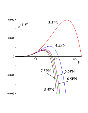
Figure 1: Some of the various PN approximants to the linear-in-spin 1SF contribution to the redshift function $z_{1}(y)$ for a spinning particle moving along a circular orbit in a Schwarzschild spacetime.

V.5 Comparison with PN results

In PN theory the linear-in-spin part of the Hamiltonian (and therefore, using Ref. Blanchet:2012at , the corresponding linear-in-spin part, $z_{1}^{(1)\hat{s}^{1}}$, of the redshift $z_{1}=\partial H/\partial m_{1}$), is known up to the next-to-next-to-leading order Levi:2015uxa . Using the results of Levi:2015uxa , we have computed $z_{1}^{(1)\hat{s}^{1}}$ as a function of $x\equiv((M+\mu)\Omega)^{2/3}$, with the following result (corresponding to the 3.5PN order):

$$z_{1}^{(1)\hat{s}^{1}}(x) = \sum_{k=2}^{\infty}C_{\chi_{1}}^{(2k+1)/2}(\nu;\ln x)\chi_{1}x^{(2k+1)/2}\,,$$

where the coefficients are given by

$$C_{\chi_{1}}^{5/2} = \frac{1}{3}\nu\Delta-\frac{1}{3}\nu+\frac{2}{3}\nu^{2}\,,$$

$$C_{\chi_{1}}^{7/2} = -\frac{1}{2}\nu\Delta+\frac{19}{18}\nu^{2}-\frac{19}{18}\nu^{2}\Delta-\frac{1}{9}\nu^{3}+\frac{1}{2}\nu\,,$$

$$C_{\chi_{1}}^{9/2} = -\frac{39}{8}\nu^{2}+\frac{11}{24}\nu^{3}\Delta+\frac{27}{8}\nu-\frac{1}{12}\nu^{4}-\frac{27}{8}\nu\Delta$$ (60)

$$-\frac{161}{24}\nu^{3}-\frac{39}{8}\nu^{2}\Delta\,.$$

Here $\chi_{1}\equiv S_{1}/\mu^{2}$, $\nu\equiv\mu M/M_{\rm tot}^{2}$ and $\Delta\equiv(M-\mu)/M_{\rm tot}=\sqrt{1-4\nu}$, with $M_{\rm tot}=M+\mu$. To convert this result into the 1SF contribution to $z_{1}(y)$, we use: $S_{1}=\mu M{\hat{s}}$, $q=\mu/M$, $\mu=M_{\rm tot}(1-\Delta)/2$, $M=M_{\rm tot}(1+\Delta)/2$, and $x=(1+q)^{2/3}y$. The first term $C_{\chi_{1}}^{5/2}$ does not contribute at the first order in $q$, i.e., at the first order in SF expansion, while the last two terms yield

$$z_{1}^{(1)\hat{s}^{1}}={\hat{s}}y^{7/2}\left(1-3y+O(y^{2})\right)q+O(q^{2})\,.$$ (61)

This agrees with the first two terms of (58), thereby providing an independent (partial) check of our result.

VI Concluding remarks

The original contribution of this paper is the formulation of the generalization of Detweiler’s redshift function $z_{1}(y)$ for a spinning particle on a circular orbit in Schwarzschild, and its first computation at a high PN-order (8.5PN, instead of the currently known 3.5PN order). The spinning particle moves here along an accelerated orbit, deviating from a timelike circular geodesics because of the spin itself which couples to the Riemann tensor of the background. We have shown how this non-geodesic character of the orbit induces in the spin-linear contribution to $z_{1}(y)$ a (gauge-dependent) term proportional to the radial gradient of $h_{kk}$ which plays a crucial role in ensuring the gauge-invariance of the final result. We have checked the gauge-invariance of our result by providing a dual calculation, in two different gauges, and in verifying that the final results agree. Our formulation opens the way to strong field numerical studies and provides a benchmark for their results. It would also be of interest to have independent investigations of the regularization procedure we use.

Another original result of this work (essential to accomplish the first result) has been the “completion” of the perturbed metric by the explicit computation (in the Regge-Wheeler gauge) of the contribution of the non-radiative multipoles to both the interior and exterior metric generated by a spinning particle. We expect this result to play a useful role in future applications.

Finally, using available PN results, we have checked the first terms of our final result.

Appendix A Low multipoles $l=0,1$

We give below the solutions for the non-radiative modes ($\ell=0$ and $\ell=1$ odd) needed for the completion of the full metric perturbation. Our approach is a generalization of well-known results of Zerilli Zerilli:1971wd to the case of a spinning particle. The $\ell=1$ even mode is essentially a gauge mode that describes a shift of the center of momentum of the system. We have checked that it does not contribute to the present calculation.

A.1 The $\ell=0$ mode

The $\ell=0$ mode is of even parity, is independent of time and represents the perturbation in the total mass-energy of the system. This was shown by Zerilli for the case of a non-spinning test particle, and our explicit calculations below show that this extends to the case of a spinning particle if one uses as additional contribution to the mass of the system the conserved Killing energy $\delta M\equiv\bar{E}$, Eq. (II), (II.1), of the spinning particle. Note that our derivation directly solves the inhomogeneous Regge-Wheeler-Zerilli equations, without using Komar-type surface integrals.

For this mode there are two gauge degrees of freedom and one can set $H_{1}=0=K$. The remaining perturbation functions $H_{0}$ and $H_{2}$ satisfy the following equations

$$\frac{dH_{2}}{dr}+\frac{H_{2}}{rf} = 2\sqrt{4\pi}\mu\frac{u^{t}}{r_{0}}\left[\delta(r-r_{0})-M\Omega_{K}\hat{s}\left(\frac{r_{0}-M}{r_{0}f_{0}}\delta(r-r_{0})+r_{0}\delta^{\prime}(r-r_{0})\right)\right]\,,$$

$$\frac{dH_{0}}{dr}+\frac{H_{2}}{rf} = 2\sqrt{4\pi}\mu\frac{M\Omega_{K}}{r_{0}\Gamma_{K}f_{0}}\hat{s}\delta(r-r_{0})\,,$$ (62)

to first order in $\hat{s}$, with solution

$$H_{0} = 2\sqrt{4\pi}\mu u^{t}\left[\frac{1}{r_{0}}(1-2{\hat{s}}M\Omega_{K})\theta(r_{0}-r)+\frac{f_{0}}{rf}\left(1+{\hat{s}}\frac{M^{2}\Omega_{K}}{r_{0}f_{0}}\right)\theta(r-r_{0})\right]\,,$$

$$H_{2} = 2\sqrt{4\pi}\mu u^{t}\left[\frac{f_{0}}{rf}\left(1+{\hat{s}}\frac{M^{2}\Omega_{K}}{r_{0}f_{0}}\right)\theta(r-r_{0})-{\hat{s}}M\Omega_{K}\delta(r-r_{0})\right]\,.$$ (63)

The nonvanishing metric components to first order in $\hat{s}$ can then be written (in terms of $\delta M\equiv\bar{E}$, Eq. (II.1)) as

$$h_{tt} = \frac{fH_{0}}{\sqrt{4\pi}}=\frac{2\mu\,\delta M}{r}\left[\frac{rf}{r_{0}f_{0}}\left(1-\frac{2r_{0}-3M}{r_{0}f_{0}}M\Omega_{K}\hat{s}\right)\theta(r_{0}-r)+\theta(r-r_{0})\right]\,,$$

$$h_{rr} = \frac{H_{2}}{\sqrt{4\pi}f}=\frac{2\mu\,\delta M}{rf^{2}}\theta(r-r_{0})-\frac{2\mu\,\delta M}{f_{0}^{2}}M\Omega_{K}{\hat{s}}\delta(r-r_{0})\,.$$ (64)

A.2 The $\ell=1$ odd mode

Similarly, we have explicitly shown, by solving the Regge-Wheeler-Zerilli field equations, that the $\ell=1$ odd mode represents the angular momentum perturbation $\delta J=\bar{J}$, Eq. (II), (II.1), added by the spinning particle to the system.

The perturbation equations for this case assume $h_{1}^{\rm(odd)}=0$, whereas $h_{0}^{{\rm(odd)}}$ is such that

$$\frac{d^{2}h_{0}^{{\rm(odd)}}}{dr^{2}}-\frac{2h_{0}^{{\rm(odd)}}}{r^{2}}=-4\mu\sqrt{3\pi}u^{t}\Omega\left[\delta(r-r_{0})-M\Omega_{K}\hat{s}\left(\delta(r-r_{0})+\frac{r_{0}}{2M}(r_{0}-M)\delta^{\prime}(r-r_{0})\right)\right]\,,$$ (65)

to first order in $\hat{s}$, with solution

$$h_{0}^{\rm(odd)}=2\sqrt{\frac{4\pi}{3}}\mu u^{t}\Omega r_{0}\left[\frac{r^{2}}{r_{0}^{2}}\left(1-\frac{1}{2}{\hat{s}}(r_{0}+M)\Omega_{K}\right)\theta(r_{0}-r)+\frac{r_{0}}{r}(1+{\hat{s}}r_{0}\Omega_{K}f_{0})\theta(r-r_{0})\right]\delta_{m,0}\,,$$ (66)

and only the $m=0$ mode is nonzero. The only nonvanishing metric component is then given (in terms of $\delta J\equiv\bar{J}$, Eq. (II.1)) by

$$h_{t\phi}=-\sqrt{\frac{3}{4\pi}}h_{0}^{{\rm(odd)}}\sin^{2}\theta=-\frac{2\mu\,\delta J}{r}\left[\frac{r^{3}}{r_{0}^{3}}\left(1-\frac{3}{2}(r_{0}-M)\Omega_{K}{\hat{s}}\right)\theta(r_{0}-r)+\theta(r-r_{0})\right]\sin^{2}\theta\,,$$ (67)

to first order in $\hat{s}$.

Appendix B MPD equations in the perturbed spacetime

In this section we briefly discuss the MPD equations in the perturbed spacetime to first-order in spin. This complementary material is left here for convenience and it will be of use in future works. Working to the first order in spin, Eqs. (3) and (4) reduce to

$$\mu\frac{{\rm D}U^{\mu}}{d\tau} = -\frac{1}{2}\,R^{\mu}{}_{\nu\alpha\beta}\,U^{\nu}\,S^{\alpha\beta}\,,$$ (68)

$$\frac{{\rm D}S^{\mu\nu}}{d\tau} = 0\,,$$ (69)

where we recall that $U^{\mu}\equiv dz^{\mu}/d\tau$, and where we have used the property $P=\mu U+O(s^{2})$ for the momentum of the particle.

Assuming that the background metric admits the Killing vector $k=\partial_{t}+\Omega\partial_{\phi}$ and that the body’s orbit is aligned with $k$, $U=u^{t}k$, implying

$$-(u^{t})^{-2}=k\cdot k=-f+\Omega^{2}r^{2}+h_{kk}\,,$$ (70)

the MPD equations become

$$\mu u^{t}\nabla_{k}k^{\mu}=-\frac{1}{2}\,R^{\mu}{}_{\nu\alpha\beta}\,k^{\nu}\,S^{\alpha\beta}\,,\quad\nabla_{U}S^{\mu\nu}=0\,.$$ (71)

Defining then the spin vector (orthogonal to both $U$ and $u\equiv P/\mu$ at the first order in spin) by spatial duality (see Eq. (6))

$$S^{\gamma}=\frac{1}{2}u^{t}k_{\sigma}\eta^{\sigma\gamma\alpha\beta}S_{\alpha\beta}\,,\qquad S^{\gamma}k_{\gamma}=0\,,$$ (72)

one finds immediately that the spin vector is parallel-propagated along $U$, $\nabla_{U}S^{\gamma}=0$. The equations of motion instead can be cast in the form

$$\mu u^{t}\nabla_{k}k^{\mu} = -\frac{1}{2}(\nabla_{\mu\beta}k_{\alpha})\,S^{\alpha\beta}$$ (73)

$$= -\frac{1}{2}(\nabla_{\mu}K_{\beta\alpha})\,S^{\alpha\beta}\,,$$

where the (antisymmetric) tensor $K_{\alpha\beta}$ is given by

$$K_{\alpha\beta}=\nabla_{\alpha}k_{\beta}=\partial_{[\alpha}k_{\beta]}\,.$$ (74)

Finally, we require that the spin vector be orthogonal to the equatorial plane, i.e.,

$$S=-se_{\hat{\theta}}\,,\qquad e_{\hat{\theta}}=\frac{1}{r}\left(1-\frac{1}{2r^{2}}h_{\theta\theta}\right)\partial_{\theta}\,.$$ (75)

The equations of motion then imply the following solution for $\Omega$

$$M\Omega=M\Omega_{K}\left[1-\frac{3}{2}{\hat{s}}M\Omega_{K}+q(\tilde{\Omega}_{1}+{\hat{s}}\tilde{\Omega}_{1{\hat{s}}})\right]\,,$$ (76)

where $\Omega_{K}\equiv\sqrt{\frac{M}{r_{0}^{3}}}$, as defined in Eq. (38) above,

$$\tilde{\Omega}_{1}=-\frac{M}{4u^{2}}[\partial_{r}h_{kk}^{(0)}]_{r=M/u}\,,$$ (77)

and

$$\tilde{\Omega}_{1{\hat{s}}} = -\frac{u^{3/2}}{4(1-2u)^{2}}h_{kk}^{(0)}+\frac{(5-12u)u^{3/2}}{4}h_{rr}^{(0)}-\frac{u^{2}(3-4u)(1-3u)}{2M(1-2u)^{2}}h_{t\phi}^{(0)}-\frac{(1-3u)(2-5u+4u^{2})u^{5/2}}{4M^{2}(1-2u)^{2}}h_{\phi\phi}^{(0)}$$

$$-\frac{M^{2}u^{-3/2}}{4}[\partial_{rr}h_{kk}^{(0)}]_{r=M/u}-\frac{M}{4u}(1-3u)[\partial_{rr}h_{\phi k}^{(0)}]_{r=M/u}+\frac{M}{4u}(1-3u)[\partial_{r\bar{\phi}}h_{rk}^{(0)}]_{r=M/u}$$

$$-\frac{1}{4}(1-3u)[\partial_{\bar{\phi}}h_{rk}^{(0)}]_{r=M/u}+\frac{Mu^{1/2}}{4(1-2u)}[\partial_{r}h_{kk}^{(0)}]_{r=M/u}-\frac{M}{4u^{2}}[\partial_{r}h_{kk}^{(1)}]_{r=M/u}$$

$$+\frac{M}{4}(1-2u)(1-3u)u^{-1/2}[\partial_{r}h_{rr}^{(0)}]_{r=M/u}+\frac{(1-3u)}{4(1-2u)}[\partial_{r}h_{t\phi}^{(0)}]_{r=M/u}+\frac{(1-3u)(2-3u)u^{3/2}}{4M(1-2u)}[\partial_{r}h_{\phi\phi}^{(0)}]_{r=M/u}\,.$$

Introducing the dimensionless frequency parameter $y=(M\Omega)^{2/3}$ gives the relation

$$y=u-{\hat{s}}u^{5/2}+q{\mathcal{F}}(u)\,,$$ (79)

where ${\mathcal{F}}(u)={\mathcal{F}}_{0}(u)+\hat{s}{\mathcal{F}}_{\hat{s}}(u)$, with

$${\mathcal{F}}_{0}(u) = \frac{2}{3}u\tilde{\Omega}_{1}(u)\,,$$

$${\mathcal{F}}_{\hat{s}}(u) = \frac{1}{3}u^{5/2}\tilde{\Omega}_{1}(u)+\frac{2}{3}u\tilde{\Omega}_{1{\hat{s}}}(u)\,.$$ (80)

This relation can be inverted to give (see Eq. (21))

$$u=\frac{y}{\left(1-\frac{3}{2}{\hat{s}}y^{3/2}\right)^{2/3}}+qf(y)\,,$$ (81)

where $f(y)=f_{0}(y)+\hat{s}f_{\hat{s}}(y)$, with

$$f_{0}(y) = -{\mathcal{F}}_{0}(y)\,,$$

$$f_{\hat{s}}(y) = -{\mathcal{F}}_{\hat{s}}(y)-\frac{5}{2}y^{3/2}{\mathcal{F}}_{0}(y)-y^{5/2}{\mathcal{F}}^{\prime}_{0}(y)\,.$$ (82)

Substituting then into Eq. (70) finally yields Eq. (24).

Appendix C Metric reconstruction in the Regge-Wheeler gauge

C.1 Solving the RWZ equations

The perturbation functions of both parity can be expressed in terms of a single unknown for each sector, satisfying the same Regge-Wheeler equation

$${\mathcal{L}}^{(r)}_{\rm(RW)}[R_{\ell m\omega}^{\rm(even/odd)}]=S_{\ell m\omega}^{\rm(even/odd)}(r)\,,$$ (83)

where ${\mathcal{L}}^{(r)}_{\rm(RW)}$ denotes the RW operator

$${\mathcal{L}}^{(r)}_{\rm(RW)} = f(r)^{2}\frac{d^{2}}{dr^{2}}+\frac{2M}{r^{2}}f(r)\frac{d}{dr}+[\omega^{2}-V_{\rm(RW)}(r)]$$ (84)

$$= \frac{d^{2}}{dr_{*}^{2}}+[\omega^{2}-V_{\rm(RW)}(r)]\,,$$

with $d/dr_{*}=f(r)d/dr$, and the RW potential

$$V_{\rm(RW)}(r)=f(r)\left(\frac{\ell(\ell+1)}{r^{2}}-\frac{6M}{r^{3}}\right)\,.$$ (85)

The source terms have the form

$$S_{\ell m\omega}^{\rm(even/odd)}(r) = c_{0}^{\ell m\omega}\delta(r-r_{0})+c_{1}^{\ell m\omega}\delta^{\prime}(r-r_{0})$$

$$+ c_{2}^{\ell m\omega}\delta^{\prime\prime}(r-r_{0})+c_{3}^{\ell m\omega}\delta^{\prime\prime\prime}(r-r_{0})\,.$$

The coefficients $c_{k}^{\ell m\omega}$, $k=0\ldots 3$ are not depending on $r$ and have the general form

$$c_{k}^{\ell m\omega}=\tilde{c}_{k}^{\ell m\omega}\delta(\omega-m\Omega)\,,$$ (87)

with $c_{3}^{\ell m\omega}\equiv 0$ in the odd case.

The Green’s function is expressed in terms of the two independent homogeneous solutions $X_{\ell\omega}^{{\rm in}}$ and $X_{\ell\omega}^{{\rm up}}$ of the RW operator as

$$G(r,r^{\prime}) = G_{\rm(in)}(r,r^{\prime})H(r^{\prime}-r)+G_{\rm(up)}(r,r^{\prime})H(r-r^{\prime})\,,$$

where

$$G_{\rm(in)}(r,r^{\prime}) = \frac{X_{\ell\omega}^{{\rm in}}(r)X_{\ell\omega}^{{\rm up}}(r^{\prime})}{W_{\ell\omega}}\,,$$

$$G_{\rm(up)}(r,r^{\prime}) = \frac{X_{\ell\omega}^{{\rm in}}(r^{\prime})X_{\ell\omega}^{{\rm up}}(r)}{W_{\ell\omega}}\,.$$ (88)

Here $W_{\ell\omega}$ denotes the (constant) Wronskian

$$W_{\ell\omega} = f(r)\biggl{[}X_{\ell\omega}^{{\rm in}}(r)\frac{d}{dr}X_{\ell\omega}^{{\rm up}}(r)-\frac{d}{dr}X_{\ell\omega}^{{\rm in}}(r)X_{\ell\omega}^{{\rm up}}(r)\biggl{]}$$ (89)

$$= {\rm const.}$$

and $H(x)$ is the Heaviside step function. Both even-parity and odd-parity solutions are then given by integrals over the corresponding (distributional) sources as

$$R^{\rm(even/odd)}_{\ell m\omega}(r)=\int dr^{\prime}\,\frac{G(r,r^{\prime})}{f(r^{\prime})}S^{\rm(even/odd)}_{\ell m\omega}(r^{\prime})\,.$$ (90)

Once the radial function is known for both parities, the perturbed metric components are then computed by Fourier anti-transforming, multiplying by the angular part and summing over $m$ (between $-\ell$ and $+\ell$), and then over $\ell$ (between $0$ and $+\infty$).

C.2 Computing $h_{kk}$

Let us consider the quantity $h_{kk}\equiv h_{\alpha\beta}k^{\alpha}k^{\beta}$, where $k=\partial_{t}+\Omega\partial_{\phi}$. In the RW gauge we have

$$h_{kk}=\sum_{\ell m}h_{kk}^{\ell m}=\sum_{\ell m}(h_{kk}^{\ell m\,\rm(even)}+h_{kk}^{\ell m\,\rm(odd)})\,,$$ (91)

where the even and odd contributions (for $\ell\geq 2$) are of the form

$$h_{kk}^{\ell m\,\rm(even)}(r_{0}) = \left|Y_{\ell m}\left(\frac{\pi}{2},0\right)\right|^{2}A_{\ell m}^{\rm even}(r_{0})J_{\rm in}(r_{0})J_{\rm up}(r_{0})\,,$$

$$h_{kk}^{\ell m\,\rm(odd)}(r_{0}) = \left|\partial_{\theta}Y_{\ell m}\left(\frac{\pi}{2},0\right)\right|^{2}A_{\ell m}^{\rm odd}(r_{0})\tilde{J}_{\rm in}(r_{0})\tilde{J}_{\rm up}(r_{0})\,,$$

once evaluated along the world line of the particle $r=r_{0}$, $\theta=\pi/2$, $\phi=\Omega t$. The coefficients $A_{\ell m}^{\rm even/odd}(r_{0})$ and

$$J_{\rm in/up}(r_{0}) = \alpha_{\rm in/up}(r_{0})X^{\rm in/up}_{\ell\omega}(r_{0})$$

$$+\beta_{\rm in/up}(r_{0})\left.\frac{dX^{\rm in/up}_{\ell\omega}}{dr}\right|_{r=r_{0}}\,,$$

$$\tilde{J}_{\rm in/up}(r_{0}) = \tilde{\alpha}_{\rm in/up}(r_{0})X^{\rm in/up}_{\ell\omega}(r_{0})$$ (92)

$$+\tilde{\beta}_{\rm in/up}(r_{0})\left.\frac{dX^{\rm in/up}_{\ell\omega}}{dr}\right|_{r=r_{0}}\,,$$

all depend on $\hat{s}$ and are known functions of $r_{0}$, with $\omega=m\Omega$.

Expanding all terms to first order in ${\hat{s}}$ and combining the odd and even contributions leads to

$$h_{kk}^{\ell m}=h_{kk\,(0)}^{\ell m}+{\hat{s}}h_{kk\,\hat{s}}^{\ell m}\,.$$ (93)

Performing the $m$-summation yields by definition

$$h_{kk}^{\ell}\equiv\sum_{m}h_{kk}^{\ell m}\,.$$ (94)

One must then finally express $r_{0}$ in terms of $y$ and $\hat{s}$ to get $h_{kk}^{\ell}(y,\hat{s})$.

References

• (1) S. L. Detweiler, “A consequence of the gravitational self-force for circular orbits of the Schwarzschild geometry,” Phys. Rev. D 77, 124026 (2008) doi:10.1103/PhysRevD.77.124026 [arXiv:0804.3529 [gr-qc]].
• (2) L. Barack and N. Sago, “Gravitational self-force correction to the innermost stable circular orbit of a Schwarzschild black hole,” Phys. Rev. Lett.  102, 191101 (2009) doi:10.1103/PhysRevLett.102.191101 [arXiv:0902.0573 [gr-qc]].
• (3) L. Barack, T. Damour and N. Sago, “Precession effect of the gravitational self-force in a Schwarzschild spacetime and the effective one-body formalism,” Phys. Rev. D 82, 084036 (2010) doi:10.1103/PhysRevD.82.084036 [arXiv:1008.0935 [gr-qc]].
• (4) L. Blanchet, S. L. Detweiler, A. Le Tiec and B. F. Whiting, “Post-Newtonian and Numerical Calculations of the Gravitational Self-Force for Circular Orbits in the Schwarzschild Geometry,” Phys. Rev. D 81, 064004 (2010) doi:10.1103/PhysRevD.81.064004 [arXiv:0910.0207 [gr-qc]].
• (5) L. Blanchet, S. L. Detweiler, A. Le Tiec and B. F. Whiting, “High-Order Post-Newtonian Fit of the Gravitational Self-Force for Circular Orbits in the Schwarzschild Geometry,” Phys. Rev. D 81, 084033 (2010) doi:10.1103/PhysRevD.81.084033 [arXiv:1002.0726 [gr-qc]].
• (6) A. Le Tiec, L. Blanchet and B. F. Whiting, “The First Law of Binary Black Hole Mechanics in General Relativity and Post-Newtonian Theory,” Phys. Rev. D 85 (2012) 064039 [arXiv:1111.5378 [gr-qc]].
• (7) A. Le Tiec, E. Barausse and A. Buonanno, “Gravitational Self-Force Correction to the Binding Energy of Compact Binary Systems,” Phys. Rev. Lett.  108, 131103 (2012) [arXiv:1111.5609 [gr-qc]].
• (8) E. Barausse, A. Buonanno and A. Le Tiec, “The complete non-spinning effective-one-body metric at linear order in the mass ratio,” Phys. Rev. D 85, 064010 (2012) [arXiv:1111.5610 [gr-qc]].
• (9) T. Damour, “Gravitational Self Force in a Schwarzschild Background and the Effective One Body Formalism,” Phys. Rev. D 81, 024017 (2010) doi:10.1103/PhysRevD.81.024017 [arXiv:0910.5533 [gr-qc]].
• (10) D. Bini and T. Damour, “Analytical determination of the two-body gravitational interaction potential at the fourth post-Newtonian approximation,” Phys. Rev. D 87, no. 12, 121501 (2013) doi:10.1103/PhysRevD.87.121501 [arXiv:1305.4884 [gr-qc]].
• (11) T. Regge and J. A. Wheeler, “Stability of a Schwarzschild singularity,” Phys. Rev.  108, 1063 (1957). doi:10.1103/PhysRev.108.1063
• (12) F. J. Zerilli, “Gravitational field of a particle falling in a schwarzschild geometry analyzed in tensor harmonics,” Phys. Rev. D 2, 2141 (1970). doi:10.1103/PhysRevD.2.2141
• (13) S. Mano, H. Suzuki and E. Takasugi, “Analytic solutions of the Regge-Wheeler equation and the post-Minkowskian expansion,” Prog. Theor. Phys.  96, 549 (1996) [gr-qc/9605057].
• (14) S. Mano, H. Suzuki and E. Takasugi, “Analytic solutions of the Teukolsky equation and their low frequency expansions,” Prog. Theor. Phys.  95, 1079 (1996) [gr-qc/9603020].
• (15) D. Bini and T. Damour, “High-order post-Newtonian contributions to the two-body gravitational interaction potential from analytical gravitational self-force calculations,” Phys. Rev. D 89, no. 6, 064063 (2014) doi:10.1103/PhysRevD.89.064063 [arXiv:1312.2503 [gr-qc]].
• (16) D. Bini and T. Damour, “Analytic determination of the eight-and-a-half post-Newtonian self-force contributions to the two-body gravitational interaction potential,” Phys. Rev. D 89, no. 10, 104047 (2014) doi:10.1103/PhysRevD.89.104047 [arXiv:1403.2366 [gr-qc]].
• (17) D. Bini and T. Damour, “Detweiler’s gauge-invariant redshift variable: Analytic determination of the nine and nine-and-a-half post-Newtonian self-force contributions,” Phys. Rev. D 91, 064050 (2015) doi:10.1103/PhysRevD.91.064050 [arXiv:1502.02450 [gr-qc]].
• (18) C. Kavanagh, A. C. Ottewill and B. Wardell, “Analytical high-order post-Newtonian expansions for extreme mass ratio binaries,” Phys. Rev. D 92, no. 8, 084025 (2015) doi:10.1103/PhysRevD.92.084025 [arXiv:1503.02334 [gr-qc]].
• (19) S. R. Dolan, N. Warburton, A. I. Harte, A. Le Tiec, B. Wardell and L. Barack, “Gravitational self-torque and spin precession in compact binaries,” Phys. Rev. D 89, no. 6, 064011 (2014) doi:10.1103/PhysRevD.89.064011 [arXiv:1312.0775 [gr-qc]].
• (20) D. Bini and T. Damour, “Two-body gravitational spin-orbit interaction at linear order in the mass ratio,” Phys. Rev. D 90, no. 2, 024039 (2014) doi:10.1103/PhysRevD.90.024039 [arXiv:1404.2747 [gr-qc]].
• (21) D. Bini and T. Damour, “Analytic determination of high-order post-Newtonian self-force contributions to gravitational spin precession,” Phys. Rev. D 91, no. 6, 064064 (2015) doi:10.1103/PhysRevD.91.064064 [arXiv:1503.01272 [gr-qc]].
• (22) S. R. Dolan, P. Nolan, A. C. Ottewill, N. Warburton and B. Wardell, “Tidal invariants for compact binaries on quasicircular orbits,” Phys. Rev. D 91, no. 2, 023009 (2015) doi:10.1103/PhysRevD.91.023009 [arXiv:1406.4890 [gr-qc]].
• (23) D. Bini and T. Damour, “Gravitational self-force corrections to two-body tidal interactions and the effective one-body formalism,” Phys. Rev. D 90, no. 12, 124037 (2014) doi:10.1103/PhysRevD.90.124037 [arXiv:1409.6933 [gr-qc]].
• (24) P. Nolan, C. Kavanagh, S. R. Dolan, A. C. Ottewill, N. Warburton and B. Wardell, “Octupolar invariants for compact binaries on quasicircular orbits,” Phys. Rev. D 92, no. 12, 123008 (2015) doi:10.1103/PhysRevD.92.123008 [arXiv:1505.04447 [gr-qc]].
• (25) See, e.g., the website http://mathworld.wolfram.com/PSLQAlgorithm.html
• (26) L. Barack and N. Sago, “Beyond the geodesic approximation: conservative effects of the gravitational self-force in eccentric orbits around a Schwarzschild black hole,” Phys. Rev. D 83, 084023 (2011) doi:10.1103/PhysRevD.83.084023 [arXiv:1101.3331 [gr-qc]].
• (27) S. Akcay, A. Le Tiec, L. Barack, N. Sago and N. Warburton, “Comparison Between Self-Force and Post-Newtonian Dynamics: Beyond Circular Orbits,” Phys. Rev. D 91, no. 12, 124014 (2015) doi:10.1103/PhysRevD.91.124014 [arXiv:1503.01374 [gr-qc]].
• (28) A. Le Tiec, “First Law of Mechanics for Compact Binaries on Eccentric Orbits,” Phys. Rev. D 92, 084021 (2015) doi:10.1103/PhysRevD.92.084021 [arXiv:1506.05648 [gr-qc]].
• (29) D. Bini, T. Damour and A. Geralico, “Confirming and improving post-Newtonian and effective-one-body results from self-force computations along eccentric orbits around a Schwarzschild black hole,” Phys. Rev. D 93, no. 6, 064023 (2016) doi:10.1103/PhysRevD.93.064023 [arXiv:1511.04533 [gr-qc]].
• (30) S. Hopper, C. Kavanagh and A. C. Ottewill, “Analytic self-force calculations in the post-Newtonian regime: eccentric orbits on a Schwarzschild background,” Phys. Rev. D 93, 044010 (2016) doi:10.1103/PhysRevD.93.044010 [arXiv:1512.01556 [gr-qc]].
• (31) D. Bini, T. Damour and A. Geralico, “New gravitational self-force analytical results for eccentric orbits around a Schwarzschild black hole,” Phys. Rev. D 93, no. 10, 104017 (2016) doi:10.1103/PhysRevD.93.104017 [arXiv:1601.02988 [gr-qc]].
• (32) S. Akcay, D. Dempsey and S. R. Dolan, “Spin-orbit precession for eccentric black hole binaries at first order in the mass ratio,” Class. Quant. Grav.  34, no. 8, 084001 (2017) doi:10.1088/1361-6382/aa61d6 [arXiv:1608.04811 [gr-qc]].
• (33) C. Kavanagh, D. Bini, T. Damour, S. Hopper, A. C. Ottewill and B. Wardell, “Spin-orbit precession along eccentric orbits for extreme mass ratio black hole binaries and its effective-one-body transcription,” Phys. Rev. D 96, no. 6, 064012 (2017) doi:10.1103/PhysRevD.96.064012 [arXiv:1706.00459 [gr-qc]].
• (34) A. Shah, Talk delivered at the 14 th Marcel Grossmann Meeting on General Relativity, University of Rome “La Sapienza” - Rome (IT), July 12-18, 2015
• (35) N. K. Johnson-McDaniel, A. G. Shah and B. F. Whiting, “Experimental mathematics meets gravitational self-force,” Phys. Rev. D 92, no. 4, 044007 (2015) doi:10.1103/PhysRevD.92.044007 [arXiv:1503.02638 [gr-qc]].
• (36) D. Bini, T. Damour and A. Geralico, “Spin-dependent two-body interactions from gravitational self-force computations,” Phys. Rev. D 92, no. 12, 124058 (2015) Erratum: [Phys. Rev. D 93, no. 10, 109902 (2016)] doi:10.1103/PhysRevD.93.109902, 10.1103/PhysRevD.92.124058 [arXiv:1510.06230 [gr-qc]].
• (37) C. Kavanagh, A. C. Ottewill and B. Wardell, “Analytical high-order post-Newtonian expansions for spinning extreme mass ratio binaries,” Phys. Rev. D 93, no. 12, 124038 (2016) doi:10.1103/PhysRevD.93.124038 [arXiv:1601.03394 [gr-qc]].
• (38) D. Bini, T. Damour and A. Geralico, “High post-Newtonian order gravitational self-force analytical results for eccentric equatorial orbits around a Kerr black hole,” Phys. Rev. D 93, no. 12, 124058 (2016) doi:10.1103/PhysRevD.93.124058 [arXiv:1602.08282 [gr-qc]].
• (39) S. Akcay, “Self-force correction to geodetic spin precession in Kerr spacetime,” Phys. Rev. D 96, no. 4, 044024 (2017) doi:10.1103/PhysRevD.96.044024 [arXiv:1705.03282 [gr-qc]].
• (40) C. Merlin, A. Ori, L. Barack, A. Pound and M. van de Meent, “Completion of metric reconstruction for a particle orbiting a Kerr black hole,” Phys. Rev. D 94, no. 10, 104066 (2016) doi:10.1103/PhysRevD.94.104066 [arXiv:1609.01227 [gr-qc]].
• (41) M. van de Meent, “Self-force corrections to the periapsis advance around a spinning black hole,” Phys. Rev. Lett.  118, no. 1, 011101 (2017) doi:10.1103/PhysRevLett.118.011101 [arXiv:1610.03497 [gr-qc]].
• (42) M. van De Meent, “The mass and angular momentum of reconstructed metric perturbations,” Class. Quant. Grav.  34, no. 12, 124003 (2017) doi:10.1088/1361-6382/aa71c3 [arXiv:1702.00969 [gr-qc]].
• (43) M. van de Meent, “Gravitational self-force on generic bound geodesics in Kerr spacetime,” arXiv:1711.09607 [gr-qc].
• (44) A. Buonanno and T. Damour, “Effective one-body approach to general relativistic two-body dynamics,” Phys. Rev. D 59, 084006 (1999) [gr-qc/9811091].
• (45) A. Buonanno and T. Damour, “Transition from inspiral to plunge in binary black hole coalescences,” Phys. Rev. D 62, 064015 (2000) [gr-qc/0001013].
• (46) T. Damour, “Coalescence of two spinning black holes: an effective one-body approach,” Phys. Rev. D 64, 124013 (2001) doi:10.1103/PhysRevD.64.124013 [gr-qc/0103018].
• (47) S. Akcay, L. Barack, T. Damour and N. Sago, “Gravitational self-force and the effective-one-body formalism between the innermost stable circular orbit and the light ring,” Phys. Rev. D 86, 104041 (2012) doi:10.1103/PhysRevD.86.104041 [arXiv:1209.0964 [gr-qc]].
• (48) M. Mathisson, “Neue mechanik materieller systemes,” Acta Phys. Polon.  6, 163 (1937).
• (49) A. Papapetrou, “Spinning test particles in general relativity. 1.,” Proc. Roy. Soc. Lond. A 209, 248 (1951). doi:10.1098/rspa.1951.0200
• (50) W. G. Dixon, “Dynamics of extended bodies in general relativity. I. Momentum and angular momentum,” Proc. Roy. Soc. Lond. A 314, 499 (1970). doi:10.1098/rspa.1970.0020
• (51) Y. Mino, M. Shibata and T. Tanaka, “Gravitational waves induced by a spinning particle falling into a rotating black hole,” Phys. Rev. D 53, 622 (1996) Erratum: [Phys. Rev. D 59, 047502 (1999)]. doi:10.1103/PhysRevD.53.622, 10.1103/PhysRevD.59.047502
• (52) T. Tanaka, Y. Mino, M. Sasaki and M. Shibata, “Gravitational waves from a spinning particle in circular orbits around a rotating black hole,” Phys. Rev. D 54, 3762 (1996) doi:10.1103/PhysRevD.54.3762 [gr-qc/9602038].
• (53) M. Saijo, K. i. Maeda, M. Shibata and Y. Mino, “Gravitational waves from a spinning particle plunging into a Kerr black hole,” Phys. Rev. D 58, 064005 (1998). doi:10.1103/PhysRevD.58.064005
• (54) M. Sasaki and H. Tagoshi, “Analytic black hole perturbation approach to gravitational radiation,” Living Rev. Rel.  6, 6 (2003) doi:10.12942/lrr-2003-6 [gr-qc/0306120].
• (55) H. Tagoshi, A. Ohashi and B. J. Owen, “Gravitational field and equations of motion of spinning compact binaries to 2.5 postNewtonian order,” Phys. Rev. D 63, 044006 (2001) doi:10.1103/PhysRevD.63.044006 [gr-qc/0010014].
• (56) G. Faye, L. Blanchet and A. Buonanno, “Higher-order spin effects in the dynamics of compact binaries. I. Equations of motion,” Phys. Rev. D 74, 104033 (2006) doi:10.1103/PhysRevD.74.104033 [gr-qc/0605139].
• (57) L. Blanchet, A. Buonanno and A. Le Tiec, “First law of mechanics for black hole binaries with spins,” Phys. Rev. D 87, no. 2, 024030 (2013) doi:10.1103/PhysRevD.87.024030 [arXiv:1211.1060 [gr-qc]].
• (58) M. Levi and J. Steinhoff, “Next-to-next-to-leading order gravitational spin-orbit coupling via the effective field theory for spinning objects in the post-Newtonian scheme,” JCAP 1601, 011 (2016) doi:10.1088/1475-7516/2016/01/011 [arXiv:1506.05056 [gr-qc]].
• (59) W. Tulczyjew, “Motion of multipole particles in general relativity theory,” Acta Phys. Polon.  18, 393 (1959).
• (60) J. Ehlers and E. Rudolph, “Dynamics of Extended Bodies in General Relativity Center-of-Mass Description and Quasirigidity,” Gen. Relativ. Gravit. 8, 197 (1977). doi:10.1007/BF00763547
• (61) D. Bini, A. Geralico and R. T. Jantzen, “Spin-geodesic deviations in the Schwarzschild spacetime,” Gen. Rel. Grav.  43, 959 (2011) doi:10.1007/s10714-010-1111-4 [arXiv:1408.4946 [gr-qc]].
• (62) S. Akcay, S. Dolan, C. Kavanagh, A. C. Ottewill, N. Warburton and B. Wardell, in preparation
• (63) A. G. Shah, J. L. Friedman and T. S. Keidl, “EMRI corrections to the angular velocity and redshift factor of a mass in circular orbit about a Kerr black hole,” Phys. Rev. D 86, 084059 (2012) doi:10.1103/PhysRevD.86.084059 [arXiv:1207.5595 [gr-qc]].