Density-Wavefunction Mapping in Degenerate Current-Density-Functional Theory

Abstract

We show that the particle density, $\rho({\mathbf{r}})$, and the paramagnetic current density, $\mathbf{j}^{p}({\mathbf{r}})$, are not sufficient to determine the set of degenerate ground-state wave functions. This is a general feature of degenerate systems where the degenerate states have different angular momenta. We provide a general strategy for constructing Hamiltonians that share the same ground state density, yet differ in degree of degeneracy. We then provide a fully analytical example for a noninteracting system subject to electrostatic potentials and uniform magnetic fields. Moreover, we prove that when $(\rho,\mathbf{j}^{p})$ is ensemble $(v,\mathbf{A})$-representable by a mixed state formed from $r$ degenerate ground states, then any Hamiltonian $H(v^{\prime},\mathbf{A}^{\prime})$ that shares this ground state density pair must have at least $r$ degenerate ground states in common with $H(v,\mathbf{A})$. Thus, any set of Hamiltonians that shares a ground-state density pair $(\rho,\mathbf{j}^{p})$ by necessity has at least have one joint ground state.

A cornerstone of modern density-functional theory (DFT) is the Hohenberg-Kohn theorem Hohenberg1964 , which states that the ground-state particle density of a quantum-mechanical system determines up to an additive constant the one-body potential $v$ of the same system. The original argument was limited to systems that have unique ground states. Although DFT can be formulated without recourse to the Hohenberg-Kohn theorem, using the constrained-search and Lieb’s convex analysis formalisms Levy ; Lieb83 , the result strengthens and adds insight to the theory. Firstly, the alternative DFT formulations establish only that densities determine various contributions to the total energy; in particular, the exchange-correlation energy, and properties given as functional derivatives of the energy with respect to the scalar potential. The stronger statement that the wave function and Hamiltonian, and consequently all properties of a system, are determined still requires the Hohenberg-Kohn theorem. Secondly, whereas alternatives are known for ground-state DFT, the available formulation of time-dependent DFT is most closely related to the Hohenberg-Kohn formulation RungeGross .
When the Hamiltonian contains a magnetic vector potential in addition to the scalar potential, the particle density alone is no longer sufficient for a rigorous formulation of DFT. The most well-established extension is current-density-functional theory (CDFT), where it has been proven that the particle density, $\rho$, and the paramagnetic current density, $\mathbf{j}^{p}$, determine the non-degenerate ground-state Vignale1987 ; Capelle2002 (see Eqs. (2) and (3) for the definition of $\rho$ and $\mathbf{j}^{p}$, respectively). We use the term weak Hohenberg-Kohn theorem (cf. Tellgren2017 , Sec. III D) for this result and, following Dreizler and Gross Dreizler , denote the invertible map from non-degenerate ground states to densities by $\mathcal{D}$. The reason for the term weak is that such a result would be implied by the stronger but false statement that $(\rho,\mathbf{j}^{p})$ determines $(v,\mathbf{A})$ Capelle2002 ; Tellgren2012 ; Laestadius2014 . Thus, the map, denoted $\mathcal{C}$, from $(v,\mathbf{A})$ to non-degenerate ground states is not invertible. The situation can be summarized as

$$(v,\mathbf{A})\stackrel{{\scriptstyle\mathcal{C}}}{{\rightarrow}}\psi\stackrel{{\scriptstyle\mathcal{D}}}{{\rightleftarrows}}(\rho,\mathbf{j}^{p})~{}.$$ (1)

The fact that the map $\mathcal{C}$ is not invertible does not preclude a density-functional formulation in terms of $\rho$ and $\mathbf{j}^{p}$. Indeed, the existence of the map $\mathcal{D}^{-1}$ in non-degenerate paramagnetic CDFT is enough to define a corresponding Hohenberg-Kohn functional Vignale1987 . Furthermore, the Hohenberg-Kohn variational principle holds for the density pair $(\rho,\mathbf{j}^{p})$ and a theory of density functionals can be based on these variables Vignale1987 ; Capelle2002 . For further discussion on the choice of variables for current-density functionals we refer to Tellgren2012 ; Laestadius2014 , see also the mathematical analyses in Laestadius2014b ; Laestadius2014c ; Kvaal2015 and the related Tellgren2017 . For the status of the Hohenberg-Kohn theorem for physical current density instead of the paramagnetic current density, we refer to previous work showing that existing attempted proofs are flawed Tellgren2012 ; Laestadius2014 and the recent progress towards a positive result using the total current density MDFT ; RUGGENTHALER .
The aim of this work is to investigate a weak Hohenberg-Kohn result in CDFT without the assumption of a unique ground state. Given an N-electron wave function $\psi$, define the particle density and the paramagnetic current density according to

$$\rho_{\psi}(\mathbf{r}_{1}) =N\int|\psi|^{2}\,d\mathbf{r}_{-1},$$ (2)

$$\mathbf{j}_{\psi}^{p}(\mathbf{r}_{1}) =N\,\text{Im}\int\overline{\psi}\,\nabla_{1}\psi\,d\mathbf{r}_{-1},$$ (3)

where $\int d\mathbf{r}_{-1}$denotes integration over all space for all but one particle and $\overline{\psi}$ denotes the complex conjugate of $\psi$. Furthermore, given a vector potential $\mathbf{A}$ we may compute the total current density as the sum $\mathbf{j}=\mathbf{j}^{p}+\rho\mathbf{A}$.
For vanishing $\mathbf{A}$, the Hohenberg-Kohn theorem states that if $\rho_{1}=\rho_{2}$, then $V_{1}=V_{2}\,+$ constant, where $V_{k}=\sum_{j}v_{k}(\mathbf{r}_{j})$ Hohenberg1964 . The proof of this result relies on the fact that if $\psi$ is a ground state of both systems, then $(V_{1}-V_{2})\psi=\text{constant}\times\psi$. If $\psi$ does not vanish on a set of positive (Lebesgue) measure, we have $V_{1}=V_{2}\,+$ constant (almost everywhere). At any rate $V_{1}=V_{2}$ up to a constant holds on the complement of $\mathcal{N}_{\psi}=\{\psi=0\}$. Assuming that the measure of $\mathcal{N}_{\psi}$ is zero (i.e., assuming that that the Schrödinger equation has the unique-continuation property from sets of positive measure), the proof can be completed by means of the variational principle as first suggested in Hohenberg1964 . A generalization of the original Hohenberg-Kohn theorem that includes degeneracy was given in Englisch1983 . [See also the work of Lammert Lammert2015 for further analysis of the set $\mathcal{N}_{\psi}$ in connection with the Hohenberg-Kohn theorem in DFT.]
In the presence of a magnetic field, a ground state $\psi$ does not uniquely determine the Hamiltonian $H$ Capelle2002 ; Tellgren2012 ; Laestadius2014 . This leads to complications in the following way: We demonstrate that a given pair $\rho$ and $\mathbf{j}^{p}$ may arise from two different pairs of $v$ and $\mathbf{A}$ that do not share the same set of ground states. This shows that the conclusion of Theorem 9 in Laestadius2014 does not hold in general. Nonetheless, any set of ground-state density matrices that have the same density pair $(\rho,\mathbf{j}^{p})$ are ground states of the same set of Hamiltonians (see also Capelle2007 and the discussion that comes before Theorem 9 in Laestadius2014 ). We furthermore prove that $(\rho,\mathbf{j}^{p})$ at least determine one ground state, and under certain assumptions, the full set. This constitutes a weak ensemble Hohenberg-Kohn result in degenerate CDFT.
In what follows, our point of departure is a quantum mechanical system of $N$ (spinless) electrons subjected to both a magnetic field and a scalar potential. The Hamiltonian is

$$H(v,\mathbf{A})=H_{0}+\sum_{j=1}^{N}\Big{(}\frac{1}{2}\{-i\nabla_{j},\mathbf{A}(\mathbf{r}_{j})\}+v(\mathbf{r}_{j})+\frac{1}{2}A(\mathbf{r}_{j})^{2}\Big{)},$$

where $\{\cdot,\cdot\cdot\}$ denotes the anti commutator and $H_{0}$ is the universal part of $H$, independent of the external potentials $v$ and $\mathbf{A}$. We let

$$H_{0}(\lambda)=\frac{1}{2}\sum_{j=1}^{N}\big{(}-\nabla_{j}^{2}+\lambda\sum_{j\neq k}r_{jk}^{-1}\big{)},\quad 0\leq\lambda\leq 1,$$

where $\lambda=1$ corresponds to fully interacting electrons and $\lambda=0$ the non-interacting case.
We start by demonstrating that $(\rho,\mathbf{j}^{p})$ does not determine the set of possibly degenerate ground states. The general idea is that for systems with cylindrical symmetry about the $z$-axis, degeneration can either be introduced or lifted by the application of an external magnetic field. For example, consider a cylindrically symmetric Hamiltonian $H(v+A^{2}/2,\mathbf{0})$ with a ground-state degeneracy, where the ground states are distinguished by different eigenvalues of $L_{z}$. The Hamiltonian $H(v,\mathbf{A})$ shares the same eigenstates, but the eigenvalue degeneracies are now lifted by the orbital Zeeman effect. At least for sufficiently weak magnetic fields along the $z$-axis, the state with minimal $L_{z}$ is then the unique ground state. The idea can also be applied in the other direction. That is, suppose a magnetic field has been tuned so that $H(v,\mathbf{A})$ has a ground state degeneracy, where the ground states are distinguished by different $L_{z}$ values. The degeneracy is then lifted in the spectrum of the Hamiltonian $H(v+A^{2}/2,\mathbf{0})$.
In order to avoid relying on numerical results, we shall focus on a two-dimensional non-interacting system of $N$ electrons subject to a magnetic field. Define $\mathbf{r}_{j}=(x_{j},y_{j})$, $v(r)=\frac{1}{2}\omega^{2}r^{2}$ and $\mathbf{A}=(B/2)(-y,x,0)$, where $B\geq 0$ is the strength of a uniform magnetic field perpendicular to the plane, i.e., $\mathbf{B}=B\mathbf{e}_{z}$. Since $\{-i\nabla_{j},\mathbf{A}(\mathbf{r}_{j})\}=BL_{z;j}$, the system’s Hamiltonian is given by

$$H=H_{0}(\lambda)+\sum_{j=1}^{N}\Big{(}\frac{B}{2}L_{z;j}+\Big{[}\frac{B^{2}}{8}+\frac{\omega^{2}}{2}\Big{]}r_{j}^{2}\Big{)}.$$ (4)

Let $\lambda=0$ such that $H_{0}=\sum_{j=1}^{N}(-\nabla_{j}^{2}/2)$. We write $H=\sum_{j=1}^{N}h_{j}$, where (dropping the index $j$) the one-electron operator $h$ is given by

$$h=-\frac{1}{2}\nabla^{2}+\frac{B}{2}L_{z}+\Big{[}\frac{B^{2}}{8}+\frac{\omega^{2}}{2}\Big{]}r^{2}.$$

Let $\tilde{\omega}=\sqrt{(B/2)^{2}+\omega^{2}}$. The eigenfunctions of $h$ in polar coordinates fulfill (see for instance Taut1994 )

$$\phi_{n,m}(r,\varphi) =Cr^{|m|}e^{im\varphi}L_{n}^{|m|}(\tilde{\omega}r^{2})e^{-\tilde{\omega}r^{2}/2},$$

where $L_{n}^{|m|}$ are the associated Laguerre polynomials, $n=0,1,\dots$ and $m=0,\pm 1,\dots$ The corresponding eigenvalues, or orbital energies, are given by

$$\varepsilon_{n,m}=(2n+1+|m|)\,\tilde{\omega}+\frac{mB}{2}.$$ (5)

The first few $\varepsilon_{n,m}$ are plotted in Fig. 1 for a fixed $\omega=\omega_{0}$.

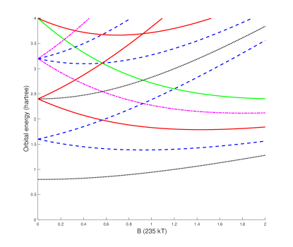
Figure 1: Orbital energies $\varepsilon_{n,m}$ (see Eq. (5)) for $\omega=0.8$ as a function of the magnetic field strength $B\geq 0$. Orbital energies with $m=0$ are shown as dotted black curves, $m=\pm 1$ as dashed blue curves, $m=\pm 2$ as solid red curves, $m=\pm 3$ as dashed dot magenta curves, and $m=\pm 4$ as solid green curves.

To prove our claim, Fig. 1 shows that it is enough to study a system with $N=3$ electrons (other particle numbers are also possible). Let $|n,m\rangle$ be the abstract state vector corresponding to the single-particle wave function $\phi_{n,m}$. Set $\omega=\omega_{0}$, $B=B_{0}=\omega_{0}/\sqrt{2}$, $e_{0}=15\omega_{0}/\sqrt{8}$ and

$$\psi_{0}^{\prime} =|0,0\rangle\otimes|0,-1\rangle\otimes|0,1\rangle,$$

$$\psi_{0} =|0,0\rangle\otimes|0,-1\rangle\otimes|0,-2\rangle,$$

where $\otimes$ denotes antisymmetrized tensor product. Then by direct computation, using $B_{0}=\omega_{0}/\sqrt{2}$,

$$H\psi_{0}^{\prime} =(\varepsilon_{0,0}+\varepsilon_{0,-1}+\varepsilon_{0,1})\psi_{0}^{\prime}=e_{0}\psi_{0}^{\prime},$$

$$H\psi_{0} =(\varepsilon_{0,0}+\varepsilon_{0,-1}+\varepsilon_{0,-2})\psi_{0}=e_{0}\psi_{0},$$

and $\psi_{0}^{\prime}$ and $\psi_{0}$ are both degenerate ground states of $H$, with energy $e_{0}$. See also Fig. 1 where $\varepsilon_{0,1}=\varepsilon_{0,-2}$ at the point $(B_{0},7B_{0}/2)\approx(0.57,1.98)$ for $\omega_{0}=0.8$. Furthermore, $L_{z}\psi_{0}^{\prime}=0$ whereas $L_{z}\psi_{0}\neq 0$.
Next, let $H^{\prime}$ be a Hamiltonian of the form (4) for a different system of the same number of electrons, but with $B=0$ and $\omega=\sqrt{(B_{0}/2)^{2}+\omega_{0}^{2}}$. It then follows from (4) that

$$H=H^{\prime}+\frac{B_{0}}{2}L_{z}.$$

Thus, $\psi_{0}^{\prime}$ is the unique ground-state (up to a phase) of $H^{\prime}$, with energy $e_{0}$. Note that the given example can be adapted to include spin. Adding the spin-Zeeman term $g\,\mathbf{B}\cdot\mathbf{s}/2$ to the one-electron operator $h$, as well as having each orbital instead doubly occupied, gives a level crossing at a different $B$ and electron number $N$.
Now, if we compute $\rho$ and $\mathbf{j}^{p}$ from just $\psi_{0}^{\prime}$, the pair $(\rho,\mathbf{j}^{p})$ is ($v,\mathbf{A}$)-representable from both $H$ and $H^{\prime}$,

$$(v,\mathbf{A})\stackrel{{\scriptstyle\mathcal{C}}}{{\rightarrow}}\{\psi_{0},\psi_{0}^{\prime}\}\rightarrow(\rho,\mathbf{j}^{p})\leftarrow\{\psi_{0}^{\prime}\}\stackrel{{\scriptstyle\mathcal{C}}}{{\leftarrow}}(v^{\prime},\mathbf{0})~{}.$$

The Hamiltonians $H$ and $H^{\prime}$ do not share the same set of ground states and consequently, we have proved: Knowledge of $\rho$ and $\mathbf{j}^{p}$ is not enough to determine the set of ground states.
In order to obtain fully analytical results, we have focused on a non-interacting model system, i.e., $\lambda=0$. Another candidate for analytical results is two-electron quantum dot with fully interacting ($\lambda=1$) electrons—we refer to the work in Taut1994 , see also Taut2009 —although the fact that exact solutions are only known for a discrete set of parameter values makes this case harder. Furthermore, level-crossings are ubituitous in more complicated systems as well. For example, quantum rings Viefers2004 , atomic systems AlHujaj2004 ; Stopkowicz2015 , and molecular systems Stopkowicz2015 ; Lange2012 all feature level crossings of the type analyzed here. The existence of level-crossings does not depend on the presence or absence of the spin-Zeeman term. In particular, the lithium atom in a homogeneous magnetic field exhibits such a level crossing: In AlHujaj2004 that includes the spin-Zeeman term (see Sec. IV A and Fig. 1, Table II and Table III), the ground-state has $L_{z}=0$ for field strengths up to a certain value after which a level crossing occurs and there are ground states with both $L_{z}=0$ and $L_{z}\neq 0$. Arguing as above, we can find a system without a magnetic field that shares the ground-state with $L_{z}=0$ and furthermore, for this system, the ground state is unique.
It is interesting to note that the above situation cannot arise for the hydrogen atom in a uniform magnetic field. Let $H=\frac{1}{2}(-i\nabla+\mathbf{A})^{2}-|{\mathbf{r}}|^{-1}$, be the Hamiltonian that models a hydrogen atom in a uniform magnetic field generated by the vector potential $\mathbf{A}=\frac{B}{2}{\mathbf{r}}_{\perp}$, $B>0$ and ${\mathbf{r}}_{\perp}=(-y,x,0)$. We denote the ground-state energy $e_{0}$ and let $\lambda_{m}=\inf_{L_{z}=m}\mathcal{R}_{H}$, where $\mathcal{R}_{H}$ is the Rayleigh-Ritz quotient of $H$, i.e.,

$$\lambda_{m}=\inf_{L_{z}=m}\frac{\langle\psi,H\psi\rangle}{\langle\psi,\psi\rangle}.$$

Theorem 4.6 in Avron1981 states $e_{0}=\lambda_{0}$, and furthermore $\lambda_{0}<\lambda_{-1}<...$ since $\lim_{|\mathbf{r}|\to 0+}v=0$. Thus, no level crossing occurs in this system.
We now turn to a positive result. To obtain a weak ensemble Hohenberg-Kohn result, denote $\Omega_{H}$ the set of ground states belonging to $H$ and let $\{\psi_{k}\}_{k=1}^{m}$ be an orthonormal basis of $\Omega_{H}$. We here assume that $m<+\infty$, i.e., the multiplicity of the ground-state energy $e_{0}$ is finite. For a basis $\{\psi_{k}\}_{k=1}^{m}$, $0\leq\lambda_{k}\leq 1$ and $\sum_{k=1}^{m}\lambda_{k}=1$, let $\Gamma_{H}(\lambda_{1},\dots,\lambda_{m})=\sum_{k=1}^{m}\lambda_{k}\psi_{k}\rangle\langle\psi_{k}$ be a density matrix of $H$. A ground-state particle density $\rho$ and paramagnetic current density $\mathbf{j}^{p}$ of $H$ are then given by $\rho=\text{Tr}\,\Gamma_{H}\hat{\rho}=\sum_{k=1}^{m}\lambda_{k}\rho_{\psi_{k}}$ and $\mathbf{j}^{p}=\text{Tr}\,\Gamma_{H}\hat{\mathbf{j}}^{p}=\sum_{k=1}^{m}\lambda_{k}\mathbf{j}_{\psi_{k}}^{p}$.
Conversely, given a particle density $\rho$ and a paramagnetic current density $\mathbf{j}^{p}$ we say that they are $(v,\mathbf{A})$-ensemble-representable if there exists $H$ with a $\Gamma_{H}$ such that $\Gamma_{H}\mapsto(\rho,\mathbf{j}^{p})$. We use the standard shorthand $\Gamma_{H}\mapsto(\rho,\mathbf{j}^{p})$ to denote $\rho=\sum_{k=1}^{m}\lambda_{k}\rho_{\psi_{k}}$ and $\mathbf{j}^{p}=\sum_{k=1}^{m}\lambda_{k}\mathbf{j}_{\psi_{k}}^{p}$. Here, of course, $\{\psi_{k}\}_{k=1}^{m}$ is a basis for $\Omega_{H}$.
We have: Suppose that $\Gamma_{k}$ is a ground-state density matrix of $H_{k}$ and moreover that $\Gamma_{k}\mapsto(\rho,\mathbf{j}^{p})$ for $k=1,2$. Then $\Gamma_{1}$ is a ground-state density matrix for $H_{2}$ and vice versa.
We can prove this claim as follows. Writing $H_{l}=H_{k}+(H_{l}-H_{k})$, we have for $l\neq k$

$$\text{Tr}\,\Gamma_{k}H_{l} =e_{k}+\int\mathbf{j}^{p}\cdot(\mathbf{A}_{l}-\mathbf{A}_{k})d\mathbf{r}$$

$$\quad+\int\rho(v_{l}-v_{k}+(A_{l}^{2}-A_{k}^{2})/2)d\mathbf{r}.$$

Consequently $\text{Tr}\,\Gamma_{1}H_{2}+\text{Tr}\,\Gamma_{2}H_{1}=e_{1}+e_{2}$. Moreover, since $e_{l}\leq\text{Tr}\,\Gamma_{k}H_{l}$ it follows $e_{l}=\text{Tr}\,\Gamma_{k}H_{l}$ and $\Gamma_{k}$ is also a ground-state density matrix of $H_{l}$. The result is illustrated in Fig. 2.

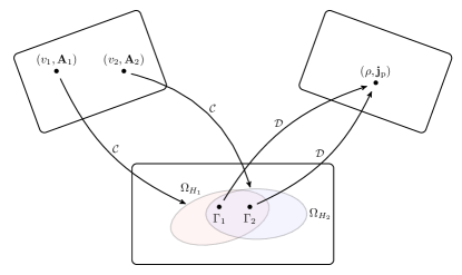
Figure 2: Two Hamiltonians have different sets of degenerate ground states (indicated by ellipses). Suppose the density matrices $\Gamma_{1}$ and $\Gamma_{2}$ are ground states of $H(v_{1},\mathbf{A}_{1})$ and $H(v_{2},\mathbf{A}_{2})$, respectively. Assume further that they map to the same density, $\Gamma_{1}\mapsto(\rho,\mathbf{j}_{p})$ and $\Gamma_{1}\mapsto(\rho,\mathbf{j}_{p})$. Then it follows that $\Gamma_{1}$ is also a ground state of $H(v_{2},\mathbf{A}_{2})$ and that $\Gamma_{2}$ is also a ground state of $H(v_{1},\mathbf{A}_{1})$. Thus, both $\Gamma_{1}$ and $\Gamma_{2}$ are located in the intersection of the two ellipses.

There are some immediate consequences of the above fact. In particular, we stress that a Hohenberg-Kohn functional can still be constructed in the degenerate case, since $F_{HK}(\rho,\mathbf{j}^{p})=\text{Tr}\,\Gamma H_{0}$ has a unique value independent of which ground state $\Gamma\mapsto(\rho,\mathbf{j}^{p})$ that is used. Furthermore, if the ground-states of $H_{1}$ and $H_{2}$ are non-degenerate, then $\rho_{1}=\rho_{2}$ and $\mathbf{j}_{1}^{p}=\mathbf{j}_{2}^{p}$ implies $\Omega_{H_{1}}=\Omega_{H_{2}}$. This is the result of Vignale and Rasolt Vignale1987 .
Returning to the degenerate case, as demonstrated in the first part of this work $\Omega_{H_{1}}=\Omega_{H_{2}}$ is not true in general even though $\Gamma_{k}\mapsto(\rho,\mathbf{j}^{p})$. We next introduce a definition. Given a $(v,\mathbf{A})$-ensemble-representable density pair $(\rho,\mathbf{j}^{p})$, there exists an $H$ with ground state $\Gamma_{H}$ such that $\rho=\text{Tr}\,\Gamma_{H}\hat{\rho}$ and $\mathbf{j}^{p}=\text{Tr}\,\Gamma_{H}\hat{\mathbf{j}}^{p}$. Let $r(\Gamma_{H})$ denote the rank of $\Gamma_{H}$, i.e., the number of nonzero eigenvalues $\lambda_{k}$ of $\Gamma_{H}$. We have the following weak ensemble Hohenberg-Kohn result:
Assume that $H_{1}$ and $H_{2}$ have the sets of ground-states $\Omega_{H_{1}}$ with (orthonormal) basis $\psi_{1},\psi_{2},\dots,\psi_{m}$ and $\Omega_{H_{2}}$ with (orthonormal) basis $\phi_{1},\phi_{2},\dots,\phi_{n}$. Assume $\Gamma_{1}\mapsto(\rho_{1},\mathbf{j}_{1}^{p})$ and $\Gamma_{2}\mapsto(\rho_{2},\mathbf{j}_{2}^{p})$, where $\Gamma_{k}$ is a ground-state density matrix of $H_{k}$. If $\rho_{1}=\rho_{2}$ and $\mathbf{j}_{1}^{p}=\mathbf{j}_{2}^{p}$, it follows that $\Omega_{H_{1}}\cap\Omega_{H_{2}}\neq\emptyset$. Moreover, with the notation $r_{k}=r(\Gamma_{k})$ then there are at least $max(r_{1},r_{2})$ linearly independent common ground states of the two systems and

$$\text{dim}\,\,\Omega_{H_{1}}\cap\Omega_{H_{2}}\geq max(r_{1},r_{2}).$$

If in addition $r_{1}=\text{dim}\,\Omega_{H_{1}}$ and $r_{2}=\text{dim}\,\Omega_{H_{2}}$, then $\Omega_{H_{1}}=\Omega_{H_{2}}$.
To prove the above, assume that $\rho_{1}=\rho_{2}=\rho$ and $\mathbf{j}_{1}^{p}=\mathbf{j}_{2}^{p}=\mathbf{j}^{p}$. For the first part, suppose $\Omega_{H_{1}}\cap\Omega_{H_{2}}=\emptyset$ and let $\{\lambda_{k}\}_{k=1}^{m}$ satisfy $0\leq\lambda_{k}\leq 1$ and $\sum_{k}\lambda_{k}=1$ such that $\rho=\sum_{k=1}^{m}\lambda_{k}\rho_{\psi_{k}}$ and $\mathbf{j}^{p}=\sum_{k=1}^{m}\lambda_{k}\mathbf{j}_{\psi_{k}}^{p}$. We then have strict inequality

$$e_{2} <\sum_{k=1}^{m}\lambda_{k}\langle\psi_{k},H_{2}\psi_{k}\rangle=e_{1}-\int\mathbf{j}^{p}\cdot(\mathbf{A}_{2}-\mathbf{A}_{1})d\mathbf{r}$$

$$\qquad+\int\rho(v_{2}-v_{1}+(A_{2}^{2}-A_{1}^{2})/2)d\mathbf{r}.$$ (6)

On the other hand, let $\{\mu_{l}\}_{l=1}^{n}$ satisfy $0\leq\mu_{l}\leq 1$ and $\sum_{l=1}^{n}\mu_{l}=1$ such that $\rho=\sum_{l=1}^{n}\mu_{l}\rho_{\phi_{l}}$ and $\mathbf{j}^{p}=\sum_{l=1}^{n}\mu_{l}\mathbf{j}_{\phi_{l}}^{p}$. Again using $\Omega_{H_{1}}\cap\Omega_{H_{2}}=\emptyset$, it holds

$$e_{1} <\sum_{l=1}^{n}\mu_{l}\langle\phi_{l},H_{1}\phi_{l}\rangle=e_{2}-\int\mathbf{j}^{p}\cdot(\mathbf{A}_{1}-\mathbf{A}_{2})d\mathbf{r}$$

$$\qquad+\int\rho(v_{1}-v_{2}+(A_{1}^{2}-A_{2}^{2})/2)d\mathbf{r}.$$ (7)

Adding (6) and (7) gives $e_{1}+e_{2}<e_{1}+e_{2}$, which is a contradiction and $\Omega_{H_{1}}\cap\Omega_{H_{2}}\neq\emptyset$.
For the second part, we use that $\Gamma_{k}\mapsto(\rho,\mathbf{j}^{p})$ implies that $\Gamma_{1}$ is a ground-state density matrix of $H_{2}$ (and vice versa). To obtain a contradiction, assume $\text{dim}\,\,\Omega_{H_{1}}\cap\Omega_{H_{2}}<r_{1}$. Without loss of generality, let $\psi_{1},\psi_{2},\dots,\psi_{m^{\prime}}\in\Omega_{H_{2}}$ and $\psi_{m^{\prime}+1},\psi_{m^{\prime}+2},\dots,\psi_{m}\notin\Omega_{H_{2}}$, where $m^{\prime}<r_{1}\leq m$. This implies

$$\text{Tr}\,\Gamma_{1}H_{2}=\left(\sum_{k=1}^{m^{\prime}}+\sum_{k=m^{\prime}+1}^{m}\right)\lambda_{k}\langle\psi_{k},H_{2}\psi_{k}\rangle>e_{2}$$

and $\Gamma_{1}$ is not a ground-state density matrix of $H_{2}$. By above, this is a contradiction. Hence, there are at least $r_{1}$ ground states $\psi_{k}\in\Omega_{H_{2}}$.
The proof that there are at least $r_{2}$ ground states $\phi_{k}\in\Omega_{H_{1}}$ is completely analogous, and we can conclude that there are at least $\max(r_{1},r_{2})$ common ground states of two systems and $\text{dim}\,\,\Omega_{H_{1}}\cap\Omega_{H_{2}}\geq\max(r_{1},r_{2})$.
Lastly, with $r_{1}=m$ and $r_{2}=n$, we obtain from the previous step

$$\min(m,n)\geq\text{dim}\,\,\Omega_{H_{1}}\cap\Omega_{H_{2}}\geq\max(m,n).$$

This can only hold when $m=n$, and consequently $\Omega_{H_{1}}=\Omega_{H_{2}}$. This completes the proof.
To summarize, we have proved that a density pair $(\rho,\mathbf{j}^{p})$ in general does not determine the full set of ground states. The counterexample we have provided demonstrates that a given $(\rho,\mathbf{j}^{p})$ may correspond to either a system with a unique ground state, or a system with degenerate ground states. All that is known is that any system that has $(\rho,\mathbf{j}^{p})$ as a ground-state density pair must at least share one ground state. While a fully analytical proof is tractable in special cases, such as noninteracting systems, the counterexample only requires that a level-crossing can be tuned by a magnetic field. Hence, this situation is common and can be established numerically in many systems, such as the lithium atom. Moreover, we have proved a positive result. When $(\rho,\mathbf{j}^{p})$ is ensemble $(v,\mathbf{A})$-representable by a mixed state formed from $r$ degenerate ground states, then any Hamiltonian $H(v^{\prime},\mathbf{A}^{\prime})$ that shares this ground state density pair must have at least $r$ degenerate ground states in common with $H(v,\mathbf{A})$. Finally, we emphasize that the complications in CDFT due to degeneracy does not effect the generalized Hohenberg-Kohn functional since any ground-state $\Gamma\mapsto(\rho,\mathbf{j}^{p})$ has the same expectation value $\text{Tr}\,\Gamma H_{0}$.

Acknowledgments. We acknowledge the support of the Norwegian Research Council through the CoE Hylleraas Centre for Quantum Molecular Sciences Grant No. 262695. Furthermore, AL acknowledges support from ERC-STG-2014 Grant Agreement No. 639508 and EIT is grateful for support by the Norwegian Research Council through the Grant No. 240674. We thank A. M. Teale for helpful comments.

References

(1)
P. Hohenberg and W. Kohn, Phys. Rev. B 1964, 136, 864.
(2)
M. Levy, Proc. Natl. Acad. Sci. U.S.A. 1979, 76, 6062.
(3)
E. H. Lieb, Int. J. Quant. Chem. 1983, 24, 243.
(4)
E. Runge and E. K. U. Gross, Phys. Rev. Lett. 1984, 52, 997.
(5)
G. Vignale and M. Rasolt, Phys. Rev. Lett. 1987, 59, 2360.
(6)
K. Capelle and G. Vignale, Phys. Rev. B 2002, 65, 113106.
(7)
E. I. Tellgren, A. Laestadius, T. Helgaker, S. Kvaal and A. M. Teale, J. Chem. Phys. 2018, 148, 024101.
(8)
R. M. Dreizler and E. K. U. Gross, Density Functional Theory; An Approach to the Quantum Many-Body Problem (Springer-Verlag 1990)
(9)
E.I. Tellgren, S. Kvaal, E. Sagvolden, U. Ekström, A. M. Teale and T.
Helgaker, Phys. Rev. A 2012, 86, 062506.
(10)
A. Laestadius and M. Benedicks, Int. J. Quant. Chem. 2014, 114, 782.
(11)
A. Laestadius, Int. J. Quant. Chem. 2014, 114, 1445.
(12)
A. Laestadius, J. Math. Chem. 2014, 52, 2581.
(13)
S. Kvaal and T. Helgaker, J. Chem. Phys. 2015, 143, 184106.
(14)
E. I. Tellgren, Phys. Rev. A 2018, 97, 012504.
(15)
M. Ruggenthaler, Ground-State Quantum-Electro-dynamical Density-Functional Theory, 2017 arXiv:1509.01417.
(16)
H. Englisch and R. Englisch, Physica A 1983, 121, 253.
(17)
P.E. Lammert, A Gamut of Hohenberg-Kohn properties 2016, preprint arXiv:1412.3876.
(18)
K. Capelle, C. A. Ullrich and G. Vignale, Phys. Rev. A 2007, 76, 012508.
(19)
M. Taut, J. Phys. A: Math. Gen. 1994, 27, 1045.
(20)
M. Taut, P. Machon and H. Eschrig, Phys. Rev. A 2009, 80, 022517.
(21)
S. Viefers, P. Koskinen, P. Singha Deo and M. Manninen, Physica E 2004, 21, 1.
(22)
O.-A. Al-Hujaj and P. Schmelcher, Phys. Rev. A 2004, 70, 033411.
(23)
S. Stopkowicz, J. Gauss, K. K. Lange, E. I. Tellgren and T. Helgaker, J. Chem. Phys. 2015, 143, 074110.
(24)
K. K. Lange, E. I. Tellgren, M. R. Hoffmann and T. Helgaker 2012, 337 327.
(25)
J. E. Avron, I. W. Herbst and B. Simon, Commun. Math. Phys. 1981, 79, 529.