Strange nucleon electromagnetic form factors from lattice QCD

Abstract

We evaluate the strange nucleon electromagnetic form factors using an ensemble of gauge configurations generated with two degenerate maximally twisted mass clover-improved fermions with mass tuned to approximately reproduce the physical pion mass. In addition, we present results for the disconnected light quark contributions to the nucleon electromagnetic form factors. Improved stochastic methods are employed leading to high-precision results. The momentum dependence of the disconnected contributions is fitted using the model-independent z-expansion. We extract the magnetic moment and the electric and magnetic radii of the proton and neutron by including both connected and disconnected contributions. We find that the disconnected light quark contributions to both electric and magnetic form factors are non-zero and at the few percent level as compared to the connected. The strange form factors are also at the percent level but more noisy yielding statistical errors that are typically within one standard deviation from a zero value.

I Introduction

The electromagnetic form factors of the nucleon are important quantities encapsulating information about the distribution of electric charge and magnetism inside the proton and neutron. Namely, at zero momentum transfer, electromagnetic form factors yield the electric charge and magnetic moment, while from the slope of the form factors at zero momentum transfer one extracts the nucleon radii. Obtaining the individual quark contributions is a major theoretical and experimental challenge, which can reveal insights on the partonic structure of the nucleon. In particular, the strange quark contribution, which is subdominant compared to the up and down quark contributions, is especially challenging to measure. The interference between the weak and electro-magnetic amplitudes leads to a parity-violating asymmetry in the elastic scattering cross section for right- and left-handed electrons, which gives information on the strange form factors. Measuring the parity-violating electroweak asymmetry in elastic scattering of polarized electrons from protons, the HAPPEX collaboration Aniol et al. (2004) extracted the linear combination of strange form factors $G^{s}_{E}+0.392G^{s}_{M}=0.014\pm 0.020\pm 0.010$ at $Q^{2}=0.48$ GeV² which was found to be compatible with zero, where $G^{s}_{E}$ is strange electric and $G^{s}_{M}$ the strange magnetic proton form factor. The A4 experiment at MAMI Maas et al. (2004) finds a combination $G^{s}_{E}+0.225G^{s}_{M}=0.039\pm 0.034$ at $Q^{2}=0.23$ GeV², slightly non-zero within errorbars, while the SAMPLE experiment Hasty et al. (2000) determined the strange magnetic form factor $G^{s}_{M}(Q^{2}=0.1)=0.14\pm 0.29\pm 0.31$ which is consistent with zero. A combined analysis of proton and neutron electromagnetic and weak form factors from elastic electron-nucleon scattering mediated by photon and $Z^{0}$ exchange provides more recent estimates for the electric and magnetic form factors (see Refs. Ahmed et al. (2012); Baunack et al. (2009); Androic et al. (2010) for some recent experimental results). These studies also deliver results consistent with zero for the strange quark contribution, and as such, provide limits on the contribution of strange quarks in the distribution of nucleon charge and magnetization.

Lattice QCD allows for a first principles calculation of the nucleon form factors. In lattice QCD, the calculation of the individual quark contributions to nucleon matrix elements requires the so called disconnected contributions, such as the one shown in Fig. 1. A number of lattice QCD calculations exist for the isovector form factors, or equivalently the combination $(G^{p}_{E,M}-G^{n}_{E,M})$, in which the disconnected contributions cancel in the isospin limit, as well as the isoscalar $(G^{p}_{E,M}+G^{n}_{E,M})$ combination neglecting disconnected contributions, of the electric and magnetic Sachs form factors using simulations with near-physical Capitani et al. (2015); Bhattacharya et al. (2014); Green et al. (2014); Alexandrou et al. (2017a) and higher than physical Alexandrou et al. (2006, 2011, 2013) pion masses. Disconnected contributions have only recently been calculated, typically using larger than physical pion masses Green et al. (2015). In this study, we evaluate both the light and strange disconnected quark loops to high-statistical precision using an ensemble of two- degenerate twisted mass fermions with a clover term with quark mass tuned to yield a pion mass of about $130$ MeV Abdel-Rehim et al. (2017). The disconnected quark loops are estimated using improved stochastic techniques for several momenta and the nucleon two-point correlation functions are computed using a number of final momenta, allowing us to obtain the form factors from multiple nucleon moving frames. We extract the magnetic moment, electric and magnetic radii by fitting the momentum dependence of the form factors to the model-independent z-expansion Hill and Paz (2010). We use the connected contributions as calculated in Ref. Alexandrou et al. (2017a) to obtain results for the total quark contributions to the nucleon electromagnetic form factors, present new results for the strange quark contributions, and update the disconnected contributions for the light quarks.

The remainder of this paper is organized as follows: In Section II, we explain how we compute the nucleon matrix element within lattice QCD and in Section III we provide the technical details of the calculation of the disconnected contributions, the analysis and results. In Section IV, a comparison with other studies is performed and in Section V we summarize and tabulate our findings.

II Lattice extraction

The electromagnetic nucleon matrix element is decomposed in terms of two parity preserving form factors, the Dirac ($F_{1}$) and Pauli ($F_{2}$) form factors, given in Minkowski space by,

$$\langle N(p^{\prime},s^{\prime})|j_{\mu}|N(p,s)\rangle=\sqrt{\frac{m_{N}^{2}}{E_{N}(\vec{p}\,^{\prime})E_{N}(\vec{p})}}\times$$

$$\bar{u}_{N}(p^{\prime},s^{\prime})\left[\gamma_{\mu}F_{1}(q^{2})+\frac{i\sigma_{\mu\nu}q^{\nu}}{2m_{N}}F_{2}(q^{2})\right]u_{N}(p,s).$$ (1)

$N(p,s)$ is the nucleon state with initial (final) momentum $p$ ($p^{\prime}$) and spin $s$ ($s^{\prime}$), with energy $E_{N}(\vec{p})$ ($E_{N}(\vec{p}\,^{\prime})$) and mass $m_{N}$. $q^{2}=q_{\mu}q^{\mu}$ is the momentum transfer squared where $q_{\mu}=(p_{\mu}^{\prime}-p_{\mu})$ and $u_{N}$ is the nucleon spinor. The vector current $j_{\mu}$ is given by

$$j_{\mu}(x)=j^{l}_{\mu}(x)+j^{s}_{\mu}(x)$$ (2)

with

$$j^{l}_{\mu}(x)=e_{u}\,\bar{u}(x)\gamma_{\mu}u(x)+e_{d}\,\bar{d}(x)\gamma_{\mu}d(x),$$ (3)

and

$$j^{s}_{\mu}(x)=e_{s}\,\bar{s}(x)\gamma_{\mu}s(x),$$ (4)

where $(e_{u},e_{d},e_{s})=(2/3,-1/3,-1/3)$ are the electric charges carried by the up, down and strange quarks respectively. In this study, we use the local vector current, therefore renormalization is necessary and has been computed non-perturbatively using the ${\rm RI^{\prime}_{MOM}}$ scheme Gockeler et al. (1999); Alexandrou et al. (2012). Lattice artifacts have been evaluated in perturbation theory to 1-loop level and all orders in the lattice spacing and have been subtracted before taking the chiral and continuum limits Alexandrou et al. (2017b).

The nucleon matrix element on the lattice requires the evaluation of three- and two-point correlation functions. The three-point function in momentum space is given by

$$C_{\mu}(\Gamma_{\nu},\vec{q},\vec{p}\,^{\prime};t_{s},t_{\rm ins},t_{0})=\sum_{\vec{x}_{\rm ins},\vec{x}_{s}}e^{i(\vec{x}_{\rm ins}-\vec{x}_{0})\cdot\vec{q}}e^{-i(\vec{x}_{s}-\vec{x}_{0})\cdot\vec{p}\,^{\prime}}\times$$

$$\operatorname{Tr}\left[\Gamma_{\nu}\langle J(t_{s},\vec{x}_{s})j_{\mu}(t_{\rm ins},\vec{x}_{\rm ins})\bar{J}(t_{0},\vec{x}_{0})\rangle\right],$$ (5)

and the two-point function is given by

$$C(\Gamma_{0},\vec{p};t_{s},t_{0})=\sum_{\vec{x}_{s}}\operatorname{Tr}\left[\Gamma_{0}\langle J(t_{s},\vec{x}_{s})\bar{J}(t_{0},\vec{x}_{0})\rangle\right]\times$$

$$e^{-i(\vec{x}_{s}-\vec{x}_{0})\cdot\vec{p}}\;,$$ (6)

where $J_{N}$ is the standard nucleon interpolating field:

$$J_{N}(\vec{x},t)=\epsilon^{abc}u^{a}(x)[u^{b\intercal}(x)C\gamma_{5}d^{c}(x)],$$ (7)

with $C=\gamma_{0}\gamma_{2}$ the charge conjugation matrix and $u$ and $d$ are the up- and the down-quark fields respectively. $\Gamma_{\nu}$ is a projector acting on spin space, with $\Gamma_{0}=\frac{1+\gamma_{0}}{4}$ projecting to unpolarized nucleons and $\Gamma_{k}=i\gamma_{5}\gamma_{k}\Gamma_{0}$ projecting to nucleons polarized in direction $k$.

The three-point function receives contributions from both quark- connected and disconnected terms. As mentioned, the connected contributions have been evaluated and presented in Ref. Alexandrou et al. (2017a) for the same ensemble as the one used here, as have preliminary results for the disconnected light quark contributions. In this work, we present a thorough analysis of the disconnected contributions, depicted in Fig. 1, updating our results for light quarks and showing results on the strange quark contributions not calculated previously. We use Osterwalder-Seiler strange quarks Osterwalder and Seiler (1978) and tune the strange quark mass to reproduce the experimental $\Omega^{-}$ mass. This yields $a\mu_{s}=0.0259(3)$, where the lattice spacing $a=0.0938(3)$ fm as determined from the nucleon mass Alexandrou and Kallidonis (2017), yielding a renormalized strange quark mass at 2 GeV in the $\overline{\rm MS}$-scheme $m_{s}^{R}=108.6(2.2)$ MeV.

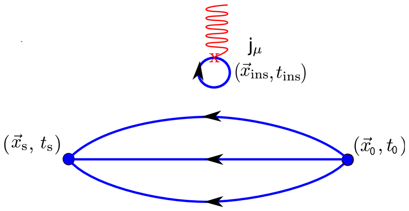
Figure 1: Disconnected three-point nucleon correlation function with source at $x_{0}$ and sink at $x_{s}$ with vector insertion $j_{\mu}$ at $x_{\rm ins}$.

To isolate the electromagnetic matrix element in the three-point function, an optimized combination of two-point functions is constructed to form the ratio,

$$R_{\mu}(\Gamma_{\nu},\vec{p}\,^{\prime},\vec{p};t_{s},t_{\rm ins})=\frac{C_{\mu}(\Gamma_{\nu},\vec{p}\,^{\prime},\vec{p};t_{s},t_{\rm ins})}{C(\Gamma_{0},\vec{p}\,^{\prime};t_{s})}\times$$

$$\sqrt{\frac{C(\Gamma_{0},\vec{p};t_{s}-t_{\rm ins})C(\Gamma_{0},\vec{p}\,^{\prime};t_{\rm ins})C(\Gamma_{0},\vec{p}\,^{\prime};t_{s})}{C(\Gamma_{0},\vec{p}\,^{\prime};t_{s}-t_{\rm ins})C(\Gamma_{0},\vec{p};t_{\rm ins})C(\Gamma_{0},\vec{p};t_{s})}}\;\;.$$ (8)

In the large time limit, $R_{\mu}(\Gamma_{\nu};\vec{p}\,^{\prime},\vec{p};t_{s};t_{\rm ins})\xrightarrow[t_{\rm ins}\rightarrow\infty]{t_{s}-t_{\rm ins}\rightarrow\infty}\Pi_{\mu}(\Gamma_{\nu};\vec{p}\,^{\prime},\vec{p})$ yielding a time independent plateau. Note that in Eq. (8), $t_{s}$ and $t_{\rm ins}$ are relative to the source, $t_{0}$, which is omitted, and we will adopt this convention for the remainder of this paper. When taking large time separations to obtain $\Pi_{\mu}(\Gamma_{\nu};\vec{p}\,^{\prime},\vec{p})$, one cannot set the source-sink time separation to arbitrarily large values since the noise-to-signal ratio grows exponentially. Therefore, one seeks a window within which the source-sink separation is large enough for the excited states to be suppressed while small enough to yield a good signal. We employ Gaussian smearing Gusken (1990); Alexandrou et al. (1994) to increase the overlap with the ground state and apply APE smearing Albanese et al. (1987) to the gauge links, with the same parameters used in Ref. Alexandrou et al. (2017a).

The Dirac and Pauli form factors, $F_{1}$ and $F_{2}$, are related to the electric Sachs ($G_{E}(Q^{2})$) and magnetic Sachs ($G_{M}(Q^{2})$) form factors via:

$$G_{E}(Q^{2})=F_{1}(Q^{2})-\frac{Q^{2}}{(2m_{N})^{2}}F_{2}(Q^{2}),$$ (9)

$$G_{M}(Q^{2})=F_{1}(Q^{2})+F_{2}(Q^{2})$$ (10)

where $Q^{2}=-q^{2}$ is the Euclidean momentum transfer squared. The combination of the projector $\Gamma_{\nu}$, the current insertion and the initial and final momenta $\vec{p}$, $\vec{p}\,^{\prime}$ leads to an overconstrained set of equations relating $\Pi_{\mu}(\Gamma_{\nu};\vec{p}\,^{\prime},\vec{p})$ to $G_{E}$ and $G_{M}$. We solve by using the Singular Value Decomposition of the minimization problem that arises. The expressions used are given in Appendix  A. The same procedure has been followed for extracting the axial and induced pseudo-scalar form factors in Ref. Alexandrou et al. (2017c), where more details can be found. For the results that follow, the analysis combines two values of the final momentum, namely $\vec{p}\,^{\prime}=\vec{0}$ and $\vec{p}\,^{\prime}=\frac{2\pi}{L}\vec{\hat{n}}$.

In what follows we use two analysis methods to assess excited states contamination and extract the matrix element of the nucleon.
Plateau method: For specific $t_{s}$ one identifies a range of $t_{\rm ins}$ where the value of the ratio remains unchanged and performs a constant fit. This procedure is repeated for several $t_{s}$ seeking for convergence in the matrix element of the ground state.
Summation method: Summing over $t_{\rm ins}$ in the ratio of Eq. (8) between the source and the sink gives,

$$\sum_{t_{\rm ins}=a}^{t_{s}-a}R_{\mu}(\Gamma_{\nu},\vec{p}\,^{\prime},\vec{p};t_{s},t_{\rm ins})=C+t_{s}\mathcal{M}+\mathcal{O}(e^{-\Delta Et_{s}})$$ (11)

where $\Delta E$ is the energy gap between the ground state and the first excited state. The nucleon matrix element, $\mathcal{M}$, is extracted from the slope by fitting to a linear form. The summation method will be used to provide an estimate of the systematic error due to potential contamination from excited states.

In Table 1 we summarize the parameters of the simulation. Details on the determination of the nucleon and pion mass and the lattice spacing are given in Ref. Alexandrou and Kallidonis (2017).

Table 1: Simulation parameters. First row gives the $\beta$-value, the value of the clover parameter $c_{\rm SW}$, the lattice spacing and the Sommer parameter $r_{0}$.

$\beta$=2.1, $c_{\rm SW}$=1.57751, $a$=0.0938(3) fm, $r_{0}/a$=5.32(5)
48${}^{3}\times$96, $L$=4.5 fm	$a\mu_{l}$=	0.0009
	$m_{\pi}$=	0.1304(4) GeV
	$m_{\pi}L$=	2.98(1)
	$m_{N}$=	0.932(4) GeV
	$m_{N}/m_{\pi}$=	7.15(4)

In Table 2 we tabulate the statistics used in this work. The disconnected quark loop entering the diagram of Fig. 1 cannot be computed exactly, except for very small lattices. In this work, we employ stochastic techniques combined with the so-called one-end trick McNeile and Michael (2006) and specifically its generalized version explained in detail in Refs. Alexandrou et al. (2017c, 2014); Abdel-Rehim et al. (2014) to estimate the disconnected quark loops. The light quark loops are produced using high-precision inversions employing deflation of the low modes to overcome critical slowdown. For the computation of strange quark loops we employ the truncated solver method (TSM) Bali et al. (2010) to increase the statistics at low cost. Details for the tuning procedure followed can be found in Ref. Alexandrou et al. (2017c). Note that we do not use any kind of dilution, therefore we invert each noise vector once.

Table 2: The statistics of our calculation. $N_{\rm conf}$ is the number of gauge configurations analyzed and $N_{\rm src}$ is the number of source positions per configuration. $N_{r}^{\rm HP}$ is the number of high-precision stochastic vectors used, and $N_{r}^{\rm LP}$ is the number of low-precision vectors used when employing the truncated solver method.

Flavor	$N_{\rm conf}$	$N_{r}^{\rm HP}$	$N_{r}^{\rm LP}$	$N_{\rm src}$
light	2120	2250	-	100
strange	2057	63	1024	100

III Analysis and results

We demonstrate the quality of our plateaus in Figs. 2 and  3. The disconnected part of the three-point function can be computed for all source-sink time separations. However, very large time separations are not useful due to the increased statistical error. Thus, we restrict to analyzing separations up to $t_{s}=1.31$ fm for which the signal-to-noise ratio is acceptable. In Fig. 2 the ratio yielding $G_{E}^{l}(Q^{2})$ is shown. Note that the upper index “${\it l}$” is used to denote the light quarks combination introduced in Eq. (3). For demonstration purposes we choose a representative momentum, namely $Q^{2}=0.0753$ GeV², having $\vec{p}\,^{\prime}=\vec{0}$.

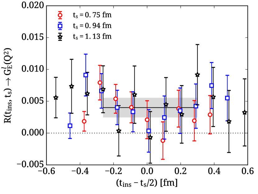
Figure 2: Results for the ratio from which $G_{E}^{l}(Q^{2})$ is extracted. This is a representative example for $Q^{2}=0.0753$ GeV². The source-sink time separations are for $t_{s}=0.75$ fm (open red circles), $t_{s}=0.94$ fm (open blue squares) and $t_{s}=1.13$ fm (open black stars). Results for the two larger separations are shifted slightly to the right for clarity. The gray band is the extracted value using the plateau method for $t_{s}=1.13$ fm, using $t_{\rm ins}$-values indicated by the length of the error band.

In Fig. 3 the ratio yielding $G_{M}^{l}(Q^{2})$ is presented. Fitting the form factors within the plateau region for several separations allows us to check convergence to the ground state. The extracted results are shown in Fig. 4 including also the result from the summation method obtained using the fit range [0.56-1.31] fm. For the case of $G_{E}^{l}$, results using the plateau method up to $t_{s}=1.13$ fm have a good agreement with the summation method while larger separations become noisy. For $G_{M}^{l}$, the value increases in magnitude as $t_{s}$ increases and becomes compatible with the summation method for $t_{s}=1.13$ fm. Therefore, we show final results extracted using the plateau method at $t_{s}=1.13$ fm to which we perform our $Q^{2}$-fits in what follows. The same procedure is followed to extract the disconnected contributions to the form factors at several $Q^{2}$ values where the analysis is extended to allow for non-zero final nucleon momentum yielding a large number of closely spaced values for $Q^{2}$. To display the results we do a weighted average on results with close values of $Q^{2}$. In particular, we use bins with width of $0.02$ GeV² for the light disconnected quark contributions and $0.04$ GeV² for the strange since for the latter we have results available up to higher $Q^{2}$ compared to the light. A systematic error due to excited states contamination is given by the difference between the plateau and the summation values.

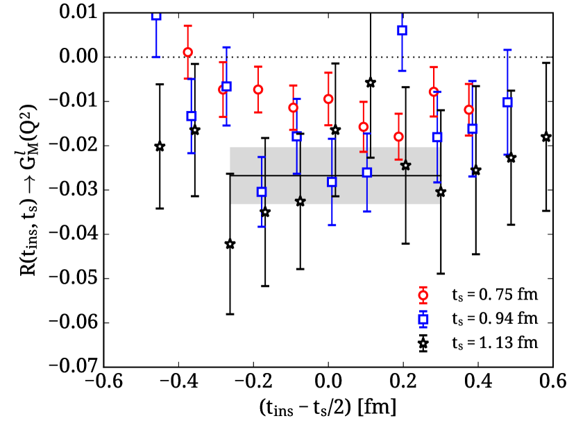
Figure 3: Ratio leading to $G_{M}^{l}(Q^{2})$ for $Q^{2}=0.0753$ GeV². The notation is as in Fig. 2.

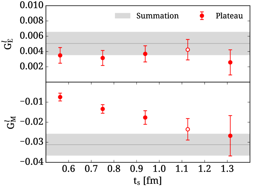
Figure 4: Extracted values for $G_{E}^{l}$ and $G_{M}^{l}$ at $Q^{2}=0.0753$ GeV² using the plateau method (red points) and summation method (gray band). Open symbols show our chosen value from the plateau method.

The dipole form is widely used to fit the proton electric and magnetic form factors Hand et al. (1963); Kelly (2004) yielding the expected behavior in the large-$Q^{2}$ region where the form factors are expected to decrease like $Q^{-4}$ Perdrisat et al. (2007). The z-expansion Hill and Paz (2010); Epstein et al. (2014) is a model independent Ansatz that has been applied recently to fit experimental results. Using a conformal mapping of $Q^{2}$ to a variable $z$ defined as,

$$z=\frac{\sqrt{t_{cut}+Q^{2}}-\sqrt{t_{cut}}}{\sqrt{t_{cut}+Q^{2}}+\sqrt{t_{cut}}}$$ (12)

one can expand the form factor into a polynomial

$$G(Q^{2})=\sum_{k=0}^{k_{max}}a_{k}z^{k},$$ (13)

where $t_{cut}$ is the cut in the time-like region of the form factor. For light disconnected form factors $t_{cut}=(2m_{\pi})^{2}$ is used while for the strange $t_{cut}=(2m_{K})^{2}$ with $m_{K}$ the kaon mass. The z-expansion should converge as we increase $k_{max}$ and the coefficients $a_{k}$ should be bounded in size for this to happen. The form factor at $Q^{2}=0$ is obtained from the first coefficient, i.e. $G(Q^{2}=0)=a_{0}$. We define the radius as,

$$r^{2}=-6\frac{dG(Q^{2})}{dQ^{2}}\Big{|}_{Q^{2}=0},$$ (14)

which is related to the second coefficient, via $r^{2}=-3a_{1}/2t_{cut}$. In the case of the proton and neutron electric form factors the mean square radius is the same as Eq. (14), whereas for the magnetic, one has to divide with the total value of the form factor at $Q^{2}=0$.

In our fitting procedure, the coefficients $a_{0},\,a_{1}$ are free to vary, while for $a_{k>1}$ we impose Gaussian priors for the series to converge. The priors are imposed using an augmented $\chi^{2}$ where the additional term is

$$\chi^{2}_{pr}=\sum_{k>1}^{k_{max}}\frac{(a_{k}-\tilde{a}_{k})^{2}}{w_{a_{k}}}$$ (15)

for parameter $a_{k}$, which is centered at $\tilde{a}_{k}$ with width $w_{a_{k}}$. To compute $\tilde{a}_{k}$ we start by setting $k_{max}=1$ to obtain an estimate for $a_{0}$ and $a_{1}$ using jackknife ensemble averages. Then, for $k_{max}=2$, $\tilde{a}_{2}$ is set to ${\rm max(|a_{0}|,|a_{1}|)}$ and the width is chosen as $w_{a_{k}}=2\,|\tilde{a}_{k}|$. This procedure is generalized for any $k_{max}$ and the priors are used to restrict $a_{k}$ inside the jackknife bins.

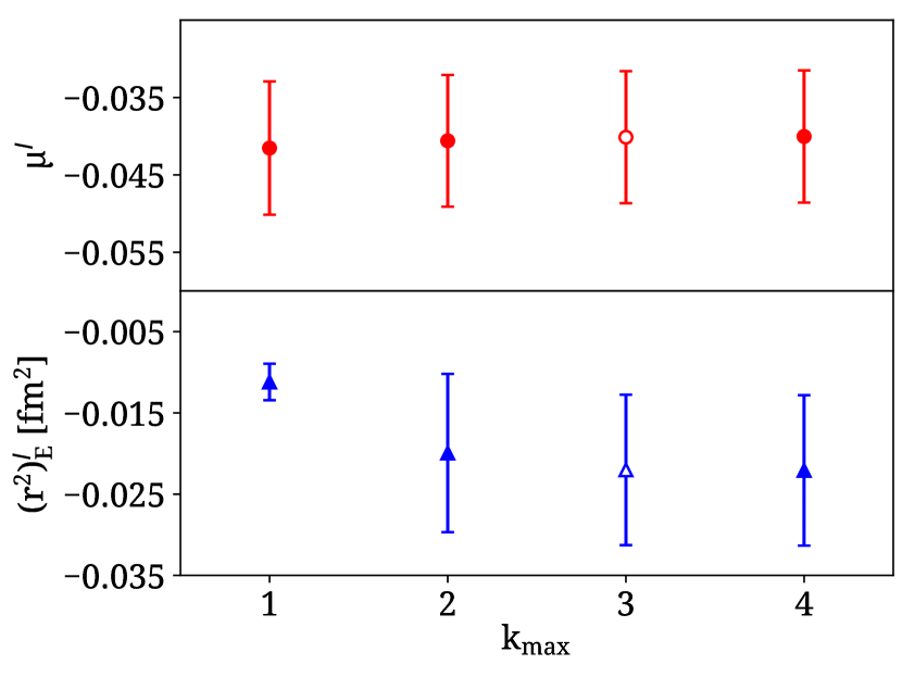
Figure 5: Extracted values for $\mu^{l}$ and $(r^{2})_{E}^{l}$ as a function of $k_{\rm max}$, where results from the plateau method at $t_{s}=1.13$ fm have been used.

In Fig. 5 we show two representative observables extracted from the electromagnetic form factors using the z-expansion as a function of $k_{\rm max}$. We seek for convergence in both mean value and error as we increase $k_{\rm max}$. In the case of the magnetic moment $\mu^{l}$, increasing $k_{\rm max}$ does not affect the result while in the case of the radius $(r^{2})_{E}^{l}$ one needs up to $k_{\rm max}=3$ to converge. Therefore, we choose to use $k_{\rm max}=3$ for all the extracted quantities where we have checked the convergence of Eq. (13).

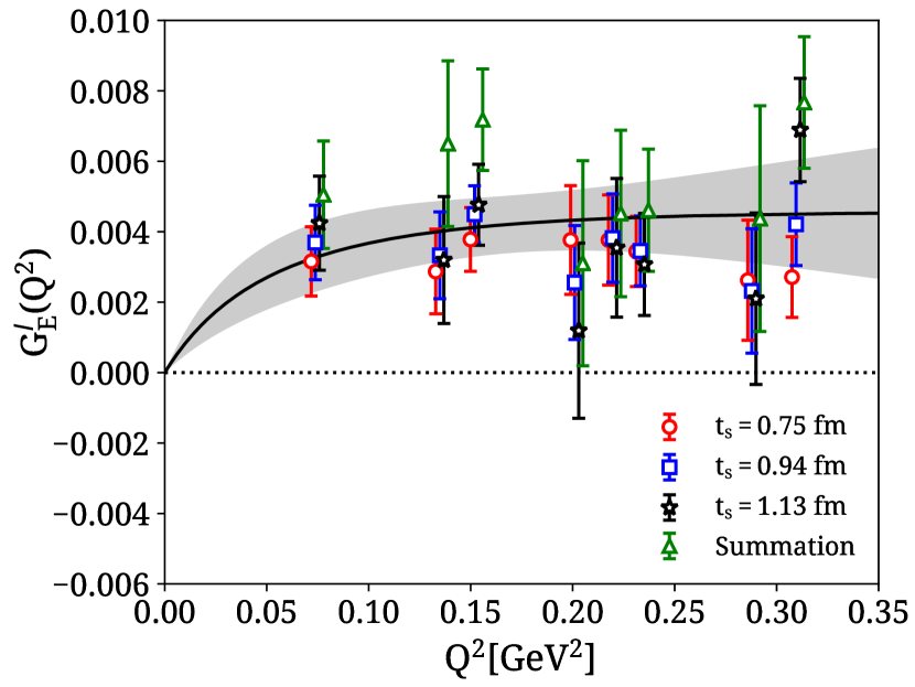
Figure 6: Disconnected light quarks contribution to the nucleon electric form factor denoted as $G_{E}^{l}(Q^{2})$. Results are extracted using the plateau method for three source-sink time separations with $t_{s}=0.75$ fm (red open circles), $t_{s}=0.94$ fm (blue open squares) and $t_{s}=1.13$ fm (black open stars). Results using the summation method in the fit range of [0.56-1.31] fm are depicted with the green open triangles. Results shown are obtained after a binning of neighboring $Q^{2}$ values as explained in the text. Results are shifted slightly to the right for clarity. The gray band is a fit to the results extracted from the plateau method using $t_{s}=1.13$ fm.

In Fig. 6 we present the light quarks disconnected contribution to the nucleon electric form factor. The form factor is shown up to $Q^{2}\sim 0.3$ GeV². The fits of the form factor yield a monotonically increasing dependence on the $Q^{2}$ that flattens out for $Q^{2}>0.2$ GeV². In the case of $G_{E}^{l}(Q^{2})$ we impose $a_{0}=0$. Fitting the results extracted from the plateau method at $t_{s}=1.13$ fm, we find a value for the radius $(r^{2})_{E}^{l}=-0.022(9)$ $\rm fm^{2}$, whereas using the summation method we find $(r^{2})_{E}^{l}=-0.035(11)$ $\rm fm^{2}$. We assign a systematic error due to possible excited states from the difference between the values extracted using the plateau and summation methods obtaining a value for the electric squared charge radius

$$(r^{2})_{E}^{l}=-0.022(9)(13)~{}\textrm{fm}^{2}.$$ (16)

It is interesting to check how much the proton and neutron charge radii are affected by the disconnected contributions. Using results for the connected contributions from Ref. Alexandrou et al. (2017a), tabulated in Table 3, we find that the connected plus disconnected light quark contributions are

$$(r^{2})_{E}^{p}(\textrm{total}) = 0.562(31)(31)~{}\textrm{fm}^{2},$$ (17)

$$(r^{2})_{E}^{n}(\textrm{total}) = -0.064(25)(14)~{}\textrm{fm}^{2}.$$ (18)

Although the light disconnected contribution to the proton charge radius is small, it is important to calculate accurately enough when comparing to experiment, especially in light of the discrepancy observed in the experimental value of proton charge radius between the conventional and the muonic hydrogen measurement. For the neutron, disconnected quark contributions are more important making the value of the charge radius more negative, albeit with large statistical errors.

In Fig. 7 we show our results for $G_{M}^{l}(Q^{2})$, which as noted above, shows a clear trend to decrease by increasing source-sink time separation, especially at small values of $Q^{2}$.

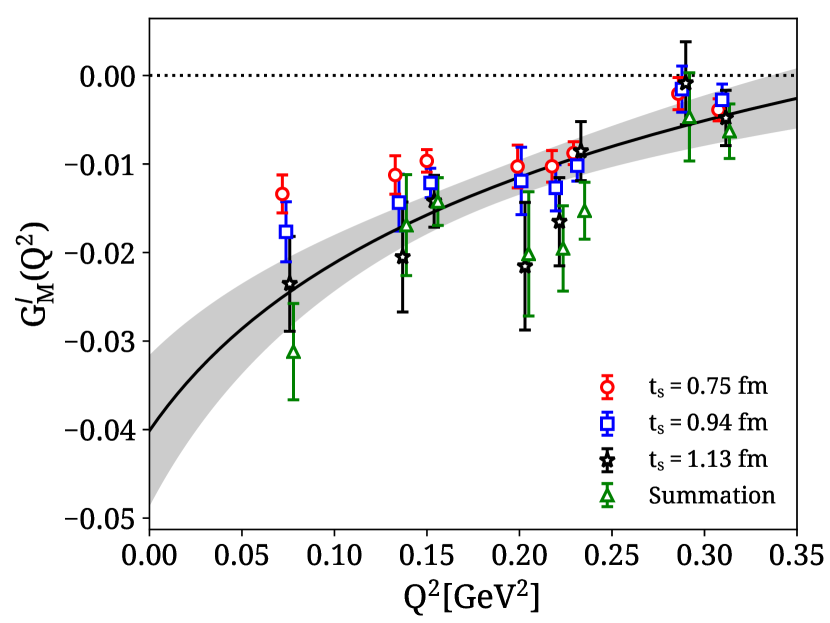
Figure 7: Disconnected light quarks contribution to the nucleon magnetic form factor $G_{M}^{l}(Q^{2})$. The notation is as in Fig. 6.

Fitting $G_{M}^{l}(Q^{2})$ using the z-expansion we find that disconnected contributions to the nucleon magnetic moment and radius are $\mu^{l}=-0.040(9)(3),\;\;\;(r^{2})^{l}_{M}=-0.071(24)(4)~{}\textrm{fm}^{2}$. In Fig. 8, we show results for the strange nucleon electric form factor, which receives only disconnected contributions. We find that the strange charge radius of the nucleon is

$$(r^{2})^{s}_{E}=0.0012(6)(7)~{}\textrm{fm}^{2},$$ (19)

which is consistent with zero if one takes into account the systematic error due to the estimate of excited state contributions.

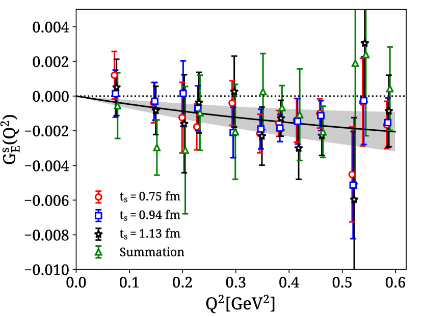
Figure 8: Strange nucleon electric form factor, $G_{E}^{s}(Q^{2})$. The notation is as in Fig. 6.

The strange magnetic form factor $G_{M}^{s}(Q^{2})$ is shown in Fig. 9. We find a strange nucleon magnetic moment of

$$\mu^{s}=0.006(4)(1).$$ (20)

The strange magnetic radius is $(r^{2})^{s}_{M}=0.0014(27)(2)~{}\textrm{fm}^{2}$, consistent with zero, as expected from the flat behavior of the form factor in Fig. 9. Our results for the proton and neutron magnetic moments and radii are given in Table 3.

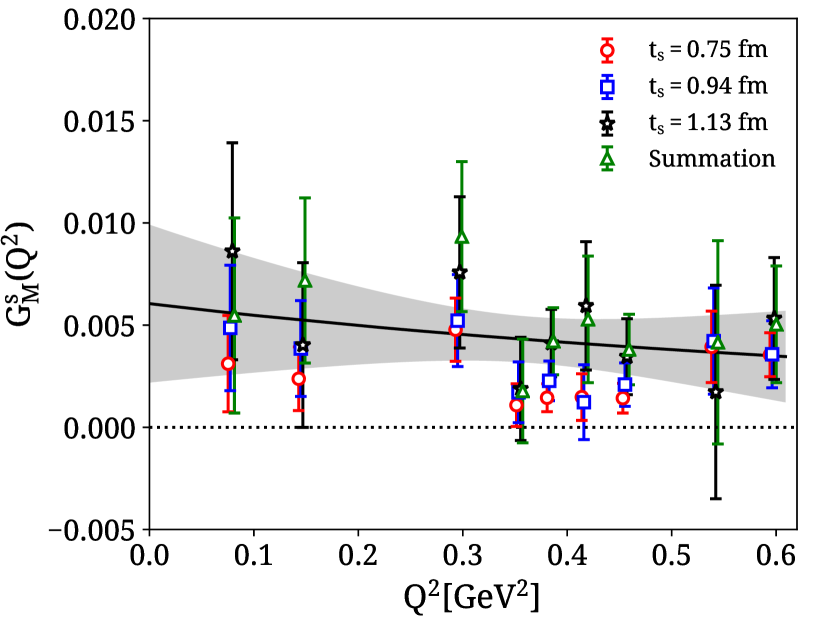
Figure 9: Strange nucleon magnetic form factor, $G_{M}^{s}(Q^{2})$. The notation is as in Fig. 6.

Table 3: Our final results for $(r^{2})_{E}$ (first row), $\mu$ (middle row) and $(r^{2})_{M}$ (last row). In the first and second columns we give the light and strange disconnected contributions, in the third and fourth, the proton connected and total values and in the fifth and sixth the corresponding ones for neutron. The radius is defined in Eq. (14). In the case of the magnetic radius one has to divide with the total value of magnetic moment to extract the mean square radius. Results for the connected are taken from Ref. Alexandrou et al. (2017a).

Quantity	Disc. light	Strange	p (conn.)	p (total)	n (conn.)	n (total)
$(r^{2})_{E}$ [fm2]	-0.022(9)(13)	0.0012(6)(7)	0.584(30)(28)	0.563(31)(31)	-0.042(23)(6)	-0.063(25)(14)
$\mu$	-0.040(9)(3)	0.006(4)(1)	2.455(127)(155)	2.421(127)(155)	-1.564(94)(123)	-1.598(95)(123)
$(r^{2})_{M}$ [fm2]	-0.071(24)(4)	0.0014(27)(2)	1.284(183)(218)	1.214(185)(218)	-0.875(139)(180)	-0.945(141)(180)

IV Comparison with other studies

Disconnected quark loop contributions to the nucleon electromagnetic form factors are available from two recent works beyond the current one. In Ref. Green et al. (2015), LHPC has analyzed an ensemble of $N_{f}=2+1$ Wilson clover-improved fermions simulated for heavier than physical pion mass, namely $m_{\pi}=317$ MeV. The other study, from $\chi$QCD, used valence overlap fermions on four $N_{f}=2+1$ domain-wall fermion ensembles with pion masses in the range $m_{\pi}\in(135,403)$ MeV Sufian et al. (2017). Their final values were extracted by performing a simultaneous chiral, infinite volume and continuum extrapolation.

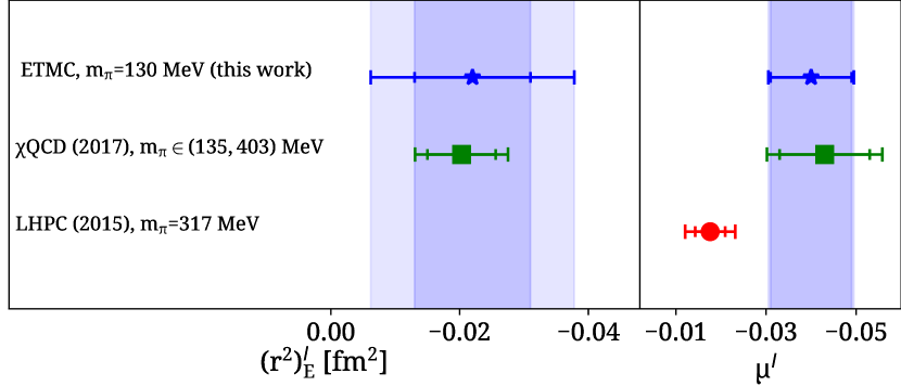
Figure 10: Comparison of our results (blue star) for $\mu^{l}$ with results from LHPC (red circle) and $\chi$QCD (green square) and for $(r^{2})^{l}_{E}$ with $\chi$QCD. We multiply by a factor of 1/3 the results from LHPC to match our convention. The inner error band is the statistical error, while the outer band is the total error.

In Fig. 10, we compare our result for $\mu^{l}$ to the one from $\chi$QCD, while for $(r^{2})^{l}_{E}$ to those from both $\chi$QCD and LHPC. The dark, inner band indicates the statistical error, while the outer band is the statistical and systematic error added in quadrature. The good agreement with $\chi$QCD, for which a continuum and infinite volume extrapolation has been performed, indicates that lattice artifacts due to finite lattice spacing and volume on these quantities are small for our ensemble. On the other hand, the result for $\mu^{l}$ from LHPC at higher than physical pion mass is smaller, as expected from chiral perturbation theory arguments. In Fig. 11 we compare the strange $\mu^{s}$ and $(r^{2})^{s}_{E}$ with the corresponding results from the two other studies. For $(r^{2})^{s}_{E}$, results from the three studies are in good agreement, whereas for $\mu^{s}$, the result from $\chi$QCD agrees within one standard deviation. Given the large statistical errors on the strange quark contributions such an agreement among lattice QCD results is welcoming.

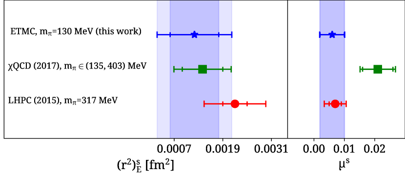
Figure 11: Comparison of our results (blue star) for $(r^{2})^{s}_{E}$ and $\mu^{s}$ with results from LHPC (red circles) and $\chi$QCD (green square). The convention is as in Fig. 10.

V Conclusions

In this study, we compute the disconnected quark loop contributions from up, down and strange quarks to the nucleon electromagnetic form factors using $N_{f}=2$ maximally twisted mass fermions at the physical point. While all source-sink time separations accessible, we opt to use up to $t_{s}=1.31$ fm for which statistical errors are not prohibitively large. Both the plateau and the summation methods are employed to estimate contamination due to the excited states. Three-point functions produced with final nucleon momenta of $\vec{p}\,^{\prime}=\vec{0}$ and $\vec{p}\,^{\prime}=\frac{2\pi}{L}\vec{\hat{n}}$ and analyzed to increase statistics. The form factors, $G_{E}^{l}(Q^{2})$ and $G_{M}^{l}(Q^{2})$, are computed up to $Q^{2}\simeq 0.3$ GeV² while $G_{E}^{s}(Q^{2})$ and $G_{M}^{s}(Q^{2})$ are computed up to $Q^{2}\simeq 0.6$ GeV². The model independent z-expansion is used to fit the $Q^{2}$ dependence of the form factors and extract the electric and magnetic radii as well as the magnetic moment. The size of the individual contributions as well as the total values for the extracted quantities are tabulated in Table 3. While the contribution of the light quark-disconnected diagram is clearly non-zero, strange quark contributions are almost consistent with zero within the current errors.

We plan to analyze an $N_{f}=2+1+1$ twisted mass ensemble with a clover term at the physical point to check possible quenching effects of the strange and charm quarks in the sea. Further improvements for the computation of disconnected quark loops are under investigation to improve the accuracy of the disconnected loop determination.

Acknowledgments: We would like to thank the members of the ETM Collaboration for a productive collaboration. We acknowledge funding from the European Union’s Horizon 2020 research and innovation program under the Marie Sklodowska-Curie Grant Agreement No. 642069.We gratefully acknowledge the Gauss Centre for Supercomputing e.V. (www.gauss-centre.eu) for funding this project by providing computing time on the GCS Supercomputer SuperMUC at Leibniz Supercomputing Centre (www.lrz.de). Results were obtained using Piz Daint at Centro Svizzero di Calcolo Scientifico (CSCS), via projects with ids s540, s625 and s702. We thank the staff of CSCS for access to the computational resources and for their constant support as well as the Jülich Supercomputing Centre (JSC) for the tape storage. MC acknowledged financial support by the US National Science Foundation under Grant No. PHY-1714407.

Appendix A Extraction of form factors from lattice QCD ratios

In this Appendix we generalize the equations from which the form factors are extracted for a nucleon with non-zero final momentum ${\vec{p}}^{\prime}$. All expressions are given in Euclidean space.

$$\Pi_{\mu}(\Gamma_{0},\vec{p}\,^{\prime},\vec{p})) = \frac{-iG_{E}(Q^{2})C}{2m(4m^{2}+Q^{2})}\left((p^{\prime}_{\mu}+p_{\mu})\left[m\left(E(\vec{p^{\prime}})+E(\vec{p})+m\right)-p^{\prime}_{\rho}p_{\rho}\right]\right)$$ (21)

$$+\frac{G_{M}(Q^{2})C}{4m^{2}(4m^{2}+Q^{2})}\Big{(}\delta_{\mu 0}\big{(}4m^{4}+m^{2}Q^{2}+4m^{2}p^{\prime}_{\rho}p_{\rho}+Q^{2}p^{\prime}_{\rho}p_{\rho}\big{)}$$

$$+2im^{2}p^{\prime}_{\mu}\big{(}E(\vec{p^{\prime}})-E(\vec{p})\big{)}-2im^{3}(p^{\prime}_{\mu}+p_{\mu})-E(\vec{p})iQ^{2}p^{\prime}_{\mu}-E(\vec{p^{\prime}})iQ^{2}p_{\mu}$$

$$-imQ^{2}(p^{\prime}_{\mu}+p_{\mu})-2im^{2}p_{\mu}\big{(}E(\vec{p^{\prime}})-E(\vec{p})\big{)}-2imp^{\prime}_{\rho}p_{\rho}(p^{\prime}_{\mu}+p_{\mu})\Big{)};$$

$$\Pi_{\mu}(\Gamma_{k},\vec{p}\,^{\prime},\vec{p})) = \frac{-G_{E}(Q^{2})C}{2m(4m^{2}+Q^{2})}\Big{(}m^{2}\varepsilon_{\mu k0\rho}(p_{\rho}^{\prime}-p_{\rho})-i\varepsilon_{\mu k\rho\sigma}p_{\rho}^{\prime}p_{\sigma}\big{(}E(\vec{p^{\prime}})+E(\vec{p})\big{)}$$ (22)

$$+\varepsilon_{\mu 0\rho\sigma}p_{\rho}^{\prime}p_{\sigma}(p_{k}^{\prime}+p_{k})-\varepsilon_{\mu k0\rho}p_{\sigma}^{\prime}p_{\sigma}(p_{\rho}^{\prime}-p_{\rho})\Big{)}$$

$$-\frac{G_{M}(Q^{2})C}{4m^{2}(4m^{2}+Q^{2})}\Big{(}m\varepsilon_{\mu k0\rho}(p_{\rho}^{\prime}-p_{\rho})(2m^{2}+Q^{2})$$

$$+2im\varepsilon_{\mu k\rho\sigma}p^{\prime}_{\rho}p_{\sigma}\big{(}2m+E(\vec{p^{\prime}})+E(\vec{p})+\frac{Q^{2}}{2m}\big{)}$$

$$-2m\varepsilon_{\mu 0\rho\sigma}p^{\prime}_{\rho}p_{\sigma}(p_{k}^{\prime}+p_{k})+2m\varepsilon_{\mu k0\rho}p^{\prime}_{\sigma}p_{\sigma}(p_{\rho}^{\prime}-p_{\rho})\Big{)},$$

where

$$C=\frac{2m}{E(\vec{p})(E(\vec{p}\,^{\prime})+m)}\sqrt{\frac{E(\vec{p})(E(\vec{p}\,^{\prime})+m)}{E(\vec{p}\,^{\prime})(E(\vec{p})+m)}}.$$ (23)

References

- Aniol et al. [2004] K. A. Aniol et al. Parity violating electroweak asymmetry in polarized-e p scattering. Phys. Rev., C69:065501, 2004. doi: 10.1103/PhysRevC.69.065501.
- Maas et al. [2004] F. E. Maas et al. Measurement of strange quark contributions to the nucleon’s form-factors at Q**2 = 0.230-(GeV/c)**2. Phys. Rev. Lett., 93:022002, 2004. doi: 10.1103/PhysRevLett.93.022002.
- Hasty et al. [2000] R. Hasty et al. Strange magnetism and the anapole structure of the proton. Science, 290:2117, 2000. doi: 10.1126/science.290.5499.2117.
- Ahmed et al. [2012] Z. Ahmed et al. New Precision Limit on the Strange Vector Form Factors of the Proton. Phys. Rev. Lett., 108:102001, 2012. doi: 10.1103/PhysRevLett.108.102001.
- Baunack et al. [2009] S. Baunack et al. Measurement of Strange Quark Contributions to the Vector Form Factors of the Proton at Q**2=0.22 (GeV/c)**2. Phys. Rev. Lett., 102:151803, 2009. doi: 10.1103/PhysRevLett.102.151803.
- Androic et al. [2010] D. Androic et al. Strange Quark Contributions to Parity-Violating Asymmetries in the Backward Angle G0 Electron Scattering Experiment. Phys. Rev. Lett., 104:012001, 2010. doi: 10.1103/PhysRevLett.104.012001.
- Capitani et al. [2015] S. Capitani, M. Della Morte, D. Djukanovic, G. von Hippel, J. Hua, B. Jäger, B. Knippschild, H. B. Meyer, T. D. Rae, and H. Wittig. Nucleon electromagnetic form factors in two-flavor QCD. Phys. Rev., D92(5):054511, 2015. doi: 10.1103/PhysRevD.92.054511.
- Bhattacharya et al. [2014] Tanmoy Bhattacharya, Saul D. Cohen, Rajan Gupta, Anosh Joseph, Huey-Wen Lin, and Boram Yoon. Nucleon Charges and Electromagnetic Form Factors from 2+1+1-Flavor Lattice QCD. Phys. Rev., D89(9):094502, 2014. doi: 10.1103/PhysRevD.89.094502.
- Green et al. [2014] J. R. Green, J. W. Negele, A. V. Pochinsky, S. N. Syritsyn, M. Engelhardt, and S. Krieg. Nucleon electromagnetic form factors from lattice QCD using a nearly physical pion mass. Phys. Rev., D90:074507, 2014. doi: 10.1103/PhysRevD.90.074507.
- Alexandrou et al. [2017a] Constantia Alexandrou, Martha Constantinou, Kyriakos Hadjiyiannakou, Karl Jansen, Christos Kallidonis, Giannis Koutsou, and Alejandro Vaquero Aviles-Casco. Nucleon electromagnetic form factors using lattice simulations at the physical point. Phys. Rev., D96(3):034503, 2017a. doi: 10.1103/PhysRevD.96.034503.
- Alexandrou et al. [2006] C. Alexandrou, G. Koutsou, John W. Negele, and A. Tsapalis. The Nucleon electromagnetic form factors from Lattice QCD. Phys. Rev., D74:034508, 2006. doi: 10.1103/PhysRevD.74.034508.
- Alexandrou et al. [2011] C. Alexandrou, M. Brinet, J. Carbonell, M. Constantinou, P. A. Harraud, P. Guichon, K. Jansen, T. Korzec, and M. Papinutto. Nucleon electromagnetic form factors in twisted mass lattice QCD. Phys. Rev., D83:094502, 2011. doi: 10.1103/PhysRevD.83.094502.
- Alexandrou et al. [2013] C. Alexandrou, M. Constantinou, S. Dinter, V. Drach, K. Jansen, C. Kallidonis, and G. Koutsou. Nucleon form factors and moments of generalized parton distributions using twisted mass fermions. Phys. Rev., D88(1):014509, 2013. doi: 10.1103/PhysRevD.88.014509.
- Green et al. [2015] Jeremy Green, Stefan Meinel, Michael Engelhardt, Stefan Krieg, Jesse Laeuchli, John Negele, Kostas Orginos, Andrew Pochinsky, and Sergey Syritsyn. High-precision calculation of the strange nucleon electromagnetic form factors. Phys. Rev., D92(3):031501, 2015. doi: 10.1103/PhysRevD.92.031501.
- Abdel-Rehim et al. [2017] A. Abdel-Rehim et al. First physics results at the physical pion mass from Wilson twisted mass fermions at maximal twist. Phys. Rev., D95(9):094515, 2017. doi: 10.1103/PhysRevD.95.094515.
- Hill and Paz [2010] Richard J. Hill and Gil Paz. Model independent extraction of the proton charge radius from electron scattering. Phys. Rev., D82:113005, 2010. doi: 10.1103/PhysRevD.82.113005.
- Gockeler et al. [1999] M. Gockeler, R. Horsley, H. Oelrich, H. Perlt, D. Petters, Paul E. L. Rakow, A. Schafer, G. Schierholz, and A. Schiller. Nonperturbative renormalization of composite operators in lattice QCD. Nucl. Phys., B544:699–733, 1999. doi: 10.1016/S0550-3213(99)00036-X.
- Alexandrou et al. [2012] C. Alexandrou, M. Constantinou, T. Korzec, H. Panagopoulos, and F. Stylianou. Renormalization constants of local operators for Wilson type improved fermions. Phys. Rev., D86:014505, 2012. doi: 10.1103/PhysRevD.86.014505.
- Alexandrou et al. [2017b] Constantia Alexandrou, Martha Constantinou, and Haralambos Panagopoulos. Renormalization functions for Nf=2 and Nf=4 twisted mass fermions. Phys. Rev., D95(3):034505, 2017b. doi: 10.1103/PhysRevD.95.034505.
- Osterwalder and Seiler [1978] K. Osterwalder and E. Seiler. Gauge Field Theories on the Lattice. Annals Phys., 110:440, 1978. doi: 10.1016/0003-4916(78)90039-8.
- Alexandrou and Kallidonis [2017] Constantia Alexandrou and Christos Kallidonis. Low-lying baryon masses using twisted mass clover-improved fermions directly at the physical pion mass. Phys. Rev., D96(3):034511, 2017. doi: 10.1103/PhysRevD.96.034511.
- Gusken [1990] S. Gusken. A Study of smearing techniques for hadron correlation functions. Nucl. Phys. Proc. Suppl., 17:361–364, 1990. doi: 10.1016/0920-5632(90)90273-W.
- Alexandrou et al. [1994] C. Alexandrou, S. Gusken, F. Jegerlehner, K. Schilling, and R. Sommer. The Static approximation of heavy - light quark systems: A Systematic lattice study. Nucl. Phys., B414:815–855, 1994. doi: 10.1016/0550-3213(94)90262-3.
- Albanese et al. [1987] M. Albanese et al. Glueball Masses and String Tension in Lattice QCD. Phys. Lett., B192:163–169, 1987. doi: 10.1016/0370-2693(87)91160-9.
- Alexandrou et al. [2017c] Constantia Alexandrou, Martha Constantinou, Kyriakos Hadjiyiannakou, Karl Jansen, Christos Kallidonis, Giannis Koutsou, and Alejandro Vaquero Aviles-Casco. Nucleon axial form factors using = 2 twisted mass fermions with a physical value of the pion mass. Phys. Rev., D96(5):054507, 2017c. doi: 10.1103/PhysRevD.96.054507.
- McNeile and Michael [2006] C. McNeile and Christopher Michael. Decay width of light quark hybrid meson from the lattice. Phys. Rev., D73:074506, 2006. doi: 10.1103/PhysRevD.73.074506.
- Alexandrou et al. [2014] C. Alexandrou, M. Constantinou, V. Drach, K. Hadjiyiannakou, K. Jansen, G. Koutsou, A. Strelchenko, and A. Vaquero. Evaluation of disconnected quark loops for hadron structure using GPUs. Comput. Phys. Commun., 185:1370–1382, 2014. doi: 10.1016/j.cpc.2014.01.009.
- Abdel-Rehim et al. [2014] A. Abdel-Rehim, C. Alexandrou, M. Constantinou, V. Drach, K. Hadjiyiannakou, K. Jansen, G. Koutsou, and A. Vaquero. Disconnected quark loop contributions to nucleon observables in lattice QCD. Phys. Rev., D89(3):034501, 2014. doi: 10.1103/PhysRevD.89.034501.
- Bali et al. [2010] Gunnar S. Bali, Sara Collins, and Andreas Schafer. Effective noise reduction techniques for disconnected loops in Lattice QCD. Comput. Phys. Commun., 181:1570–1583, 2010. doi: 10.1016/j.cpc.2010.05.008.
- Hand et al. [1963] L. N. Hand, D. G. Miller, and Richard Wilson. Electric and Magnetic Formfactor of the Nucleon. Rev. Mod. Phys., 35:335, 1963. doi: 10.1103/RevModPhys.35.335.
- Kelly [2004] J. J. Kelly. Simple parametrization of nucleon form factors. Phys. Rev., C70:068202, 2004. doi: 10.1103/PhysRevC.70.068202.
- Perdrisat et al. [2007] C. F. Perdrisat, V. Punjabi, and M. Vanderhaeghen. Nucleon Electromagnetic Form Factors. Prog. Part. Nucl. Phys., 59:694–764, 2007. doi: 10.1016/j.ppnp.2007.05.001.
- Epstein et al. [2014] Zachary Epstein, Gil Paz, and Joydeep Roy. Model independent extraction of the proton magnetic radius from electron scattering. Phys. Rev., D90(7):074027, 2014. doi: 10.1103/PhysRevD.90.074027.
- Sufian et al. [2017] Raza Sabbir Sufian, Yi-Bo Yang, Jian Liang, Terrence Draper, and Keh-Fei Liu. Sea Quarks Contribution to the Nucleon Magnetic Moment and Charge Radius at the Physical Point. Phys. Rev., D96(11):114504, 2017. doi: 10.1103/PhysRevD.96.114504.