Perturbed thermodynamics and thermodynamic geometry of a static black hole in $f(R)$ gravity

Abstract

In this paper, we consider a static black hole in $f(R)$ gravity. We recapitulate the expression for corrected thermodynamic entropy of this black hole due to small fluctuations around equilibrium. Also, we study the geometrothermodynamics (GTD) of this black hole and investigate the adaptability of the curvature scalar of geothermodynamic methods with phase transition points of this black hole. Moreover, we study the effect of correction parameter on thermodynamic behaviour of this black hole. We observe that the singular point of the curvature scalar of Ruppeiner metric coincides completely with zero point of the heat capacity and the deviation occurs with increasing correction parameter.

1 Introduction

The thermodynamics of black holes is a subject of interest these days. Thermodynamic quantities of black holes such as temperature, entropy and heat capacity; thermodynamic properties such as phase transitions and thermal stability; geometrical quantities such as horizon area and surface gravity; thermodynamical variable such as cosmological constant have been studied in several papers  [1, 2, 3, 4, 5, 6, 7, 8, 9, 10, 11, 12, 13, 14, 15, 16, 17, 18, 19, 20, 21, 22, 23, 24, 25]. Geometrical thermodynamics is other applied and important method to study phase transition of black holes. For present different implications of geometry in to usual thermodynamics, many endeavour are presented in various articles [26, 27, 28, 29, 30, 31, 32]. It is well-known that the larger black holes in comparison to the Planck scale have entropy proportional to its horizon area, so it is important to investigate the form of entropy as one reduces the size of the black hole [33, 34, 35, 36, 37, 38]. It is found that the area-law of entropy of a thermodynamic system gets correction due to the fluctuations around equilibrium [38]. These corrections are evaluated through both microscopically and using a stringy embedding of the Kerr/CFT correspondence [39]. The leading-order correction to the entropy area-law is also estimated through the Cardy formula [40]. Various check-ups confirm that the entropy due to the perturbation around thermal equilibrium of the black hole has logarithmic correction.

The study of fluctuations to the black holes thermodynamics is a subject of current interests. For instance, the thermal fluctuations corrects the thermodynamics of higher dimensional AdS black hole, where it has been found that the Van der Waals black hole is completely stable in presence of the logarithmic correction [41]. The leading-order corrections to the Gibbs free energy, charge and total mass densities of charged quasitopological and charged rotating quasitopological black holes due to thermal fluctuation are derived, where the stability and bound points of such black holes under effect of leading-order corrections are also discussed [42]. The effect of thermal fluctuations on the thermodynamics of a black geometry with hyperscaling violation is also studied recently [43]. The thermal corrections on the thermodynamics and stability of Schwarzschild-Beltrami-de Sitter black hole [44], non-rotating BTZ black hole [45], charged rotating AdS black holes [46], Gödel black hole [47], and massive black hole [48] have been investigated recently. Also, the effects of thermal fluatuation on the Hořava-Lifshitz black hole thermodynamics and their stability are discussed [49]. The leading-order correction to modified Hayward black hole is derived and found that correction term reduces the pressure and internal energy of the Hayward black hole [50].

On the other hand, in order to introduce concepts of geometry into ordinary thermodynamics many efforts have been made. In this regard, the implication of thermodynamic phase space as a differential manifold is defined, which embeds a special subspace of thermodynamic equilibrium states [26]. Many different perspective with different goals and reviews in $f(R)$ gravity have been studied in the past decade until now [51, 52, 53, 54, 55, 56, 57, 59, 58, 60]. Keeping importance of $f(R)$ gravity in mind, our motivation is to study the effect of thermal fluctuation on the thermodynamics and thermodynamic geometry of a static black hole in $f(R)$ gravity.

In this paper, we obtain corrected thermodynamic entropy and investigate thermodynamic quantities and thermodynamic geometric methods for a black holes in $f(R)$ gravity. We find that the Hawking temperature is a decreasing function of horizon radius. In order to evaluate the correction to the entropy of a static black hole in $f(R)$ gravity due to thermal fluctuation, we exploit the expressions of Hawking temperature and uncorrected specific heat. Moreover, utilizing standard thermodynamical relation, we compute first-order corrected mass and heat capacity. Here, we observe that the uncorrected mass of the black hole has a maximum value at $r_{+}=r_{m}=2.31$, and takes zero value at two points, $r_{+}=0$ and $r_{+}=4$. For the corrected mass with positive correction coefficient $\alpha$, the number of zero points of mass are not changing, but they appear with larger horizon radius. In case of heat capacity, we find that the uncorrected heat capacity is in the negative region (unstable phase) for $0<r_{+}<r_{m}$ and it takes type one phase transition at $r_{+}=r_{m}$ for which $C(r_{+}=r_{m})=0$. For $r_{+}>r_{m}$, it becomes positive valued (stable). So, without considering thermal fluctuation, this black hole has a type one phase transition. However, as long as we turn on effects of thermal fluctuation, the number of zero points of the heat capacity changes to the three zero points. Furthermore, we analyse the thermodynamic geometry of such black holes. In order to do so, we plot thermodynamic quantities and curvature scalar of Weinhold, Ruppeiner and GTD methods in terms of horizon radius. We find that the singular points of curvature scalar of Weinhold and GTD methods, for both with and without thermal fluctuations, are not coinciding with zero point of heat capacity (the phase transition points) which suggests that we are unable to get any physical information about the system with these two methods. However, without considering correction, we find that the heat capacity has only one zero, and the singular point of the curvature scalar of Ruppeiner metric is completely coinciding with it. The heat capacity under the effects of thermal fluctuation has three zero points and not all the singular points of the curvature scalar of Ruppeiner metric are not completely coinciding with zero points of such black hole but only one of the singular point of the curvature scalar of Ruppeiner metric is completely coincide with one of the zero point of the heat capacity. This suggests that, by increasing $\alpha$, the above adaptation is reducing.

This paper is organized as follows, in Sec. 2, we recapitulate the expression for corrected thermodynamic entropy of black hole due to small fluctuations around equilibrium, Then, in Sec. 3, we briefly review the static $f(R)$ black hole solution and its thermodynamics. Also, we study modified thermodynamics due to thermal fluctuations and thermodynamic geometry methods for this black hole. We conclude our results in Sec. 4.

2 Entropy under thermal fluctuation

In this section, we recapitulate the expression for corrected thermodynamic entropy of black holes due to small fluctuations around equilibrium. To do so, let us begin by defining the density of states with fixed energy as [61, 62]

$$\rho(E)=\frac{1}{2\pi i}\int_{c-i\infty}^{c+i\infty}e^{{\cal S}(\beta)}d\beta,$$ (2.1)

where the exact entropy, ${\cal S}(\beta)=\log Z(\beta)+\beta E$, depends on temperature $T(=\beta^{-1})$ explicitly. So, this (exact entropy) is not just its value at equilibrium. The exact entropy corresponds to the sum of entropies of subsystems of the thermodynamical system. This thermodynamical systems are small enough to be considered in equilibrium. To investigate the form of exact entropy, we solve the complex integral (2.1) by considering the method of steepest descent around the saddle point $\beta_{0}(={T_{H}^{-1}})$ such that $\left.\frac{\partial{\cal S}(\beta)}{\partial\beta}\right|_{\beta=\beta_{0}}=0$. Now, performing Taylor expansion of exact entropy around the saddle point $\beta=\beta_{0}$ leads to

$${\cal S}(\beta)={\cal S}_{0}+\frac{1}{2}(\beta-\beta_{0})^{2}\left(\frac{\partial^{2}{\cal S}(\beta)}{\partial\beta^{2}}\right)_{\beta=\beta_{0}}+\mbox{(higher order terms)}.$$ (2.2)

Here ${\cal S}_{0}(={\cal S}(\beta_{0}))$ is the leading-order entropy. With this value of ${\cal S}(\beta)$, the density of states (2.1 becomes

$$\rho(E)=\frac{e^{{\cal S}_{0}}}{2\pi i}\int_{c-i\infty}^{c+i\infty}\exp\left[\frac{1}{2}(\beta-\beta_{0})^{2}\left(\frac{\partial^{2}{\cal S}(\beta)}{\partial\beta^{2}}\right)_{\beta=\beta_{0}}\right]d\beta.$$ (2.3)

This further leads to [38]

$$\rho(E)=\frac{e^{{\cal S}_{0}}}{\sqrt{2\pi\left(\frac{\partial^{2}{\cal S}(\beta)}{\partial\beta^{2}}\right)_{\beta=\beta_{0}}}},$$ (2.4)

where $c=\beta_{0}$ and $\left.\frac{\partial^{2}{\cal S}(\beta)}{\partial\beta^{2}}\right|_{\beta=\beta_{0}}>0$ are chosen.

Taking logarithm of above density of states yields the microcanonical entropy density due to the small fluctuations around thermal equilibrium

$$S={\cal S}_{0}-\frac{1}{2}\log\left(\frac{\partial^{2}{\cal S}(\beta)}{\partial\beta^{2}}\right)_{\beta=\beta_{0}}+\mbox{(sub-leading terms)}.$$ (2.5)

One can determine the form of $\left.\frac{\partial^{2}{\cal S}(\beta)}{\partial\beta^{2}}\right|_{\beta=\beta_{0}}$ by considering the most general form of the exact entropy density ${\cal S}(\beta)$. Das et al. in [38] have found the form of $\left.\frac{\partial^{2}{\cal S}(\beta)}{\partial\beta^{2}}\right|_{\beta=\beta_{0}}=C_{0}T_{H}^{2}$, which leads to the leading-order corrected entropy as

$$S={\cal S}_{0}-\frac{1}{2}\ln(C_{0}T_{H}^{2}),$$ (2.6)

where $C_{0}=\left(\frac{\partial E}{\partial T}\right)_{T_{H}}$ is specific heat and $T_{H}$ is Hawking temperature. Now, a general expression for the corrected entropy can be written as following:

$$S={\cal S}_{0}-\alpha\ln(C_{0}T_{H}^{2}).$$ (2.7)

Here we introduced a parameter $\alpha$ by hand to track corrected terms where $\alpha$ can have two values either $0$ or $0.5$. In case of $\alpha=0$ we have original results and for $\alpha=0.5$ we have corrected entropy. Now, we would like to study the effects of such correction term on the thermodynamic geometry of black holes in $f(R)$ gravity.

3 Corrected thermal behaviour of a static black hole in $f(R)$ gravity

In this section we briefly review the static $f(R)$ black hole solution and its thermodynamics. The generic form of the action (in unit $G=c=\hbar=\kappa=1$) is given by

$$I=\frac{1}{2}\int d^{4}{x}\sqrt{-g}f(R)+S_{mat},$$ (3.1)

where $S_{mat}$ refers to the matter part of the action and expression for $f(R)$ gravity is considered as

$$f(R)=R+\Lambda+\frac{R+\Lambda}{R/R_{0}+2/\eta}\ln\frac{R+\Lambda}{C}.$$ (3.2)

Here $\Lambda$ is the cosmological constant, $C$ is integration constant and $R_{0}=6\eta^{2}/d^{2}$ with free parameters $\eta$ and $d$. The spherically symmetric solution of the field equations of the action (3.1) is

$$ds^{2}=-B(r)dt^{2}+B(r)^{-1}dr^{2}+r^{2}(d\theta^{2}+\sin^{2}\theta d\varphi^{2}),\quad$$ (3.3)

where

$$B(r)=1-\frac{2m}{r}+\beta_{1}r-\frac{1}{3}\Lambda{r}^{2},$$ (3.4)

here parameter $m$ is related to the mass of the black hole, $\Lambda$ is the cosmological constant and $\beta_{1}$ is a real constant [63, 64]. Eqs. (3.3) and (3.4), for $\beta_{1}=0$, convert to the space time of Schwarzschild AdS black hole and for $\beta_{1}=0$ and $\Lambda=0$, represent the Schwarzschild black hole. If $r_{+}$ denotes the radius of the event horizon, by setting $B(r)=0$, the mass of the black hole, using the relation between entropy ${\cal S}_{0}$ and event horizon radius $r_{+}$, $({\cal S}_{0}=\pi r^{2}_{+})$, is given by

$${M}_{0}({\cal S}_{0},l,\beta)=\frac{l^{2}\pi^{1/2}\beta_{1}{\cal S}_{0}+l^{2}\pi{\cal S}_{0}^{1/2}-{\cal S}_{0}^{3/2}}{2l^{2}\pi^{3/2}},$$ (3.5)

where parameter $l$ is related to the cosmological constant $\Lambda$ as follows  [65],

$$\Lambda=\frac{3}{l^{2}}.$$ (3.6)

The Hawking temperature ($T_{H}=\frac{\partial{M_{0}}}{\partial{\cal S}_{0}}$) and heat capacity ($C_{0}=T_{H}\frac{\partial{\cal S}_{0}}{\partial T_{H}}$) are calculated as [66]

$$T_{H} = \frac{2\beta_{1}l^{2}\pi^{1/2}{\cal S}_{0}^{1/2}-3{\cal S}_{0}+l^{2}\pi}{4\pi^{3/2}l^{2}{\cal S}_{0}^{1/2}},$$ (3.7)

$$C_{0} = -\frac{4\beta_{1}l^{2}\pi^{1/2}{\cal S}_{0}^{3/2}-6{\cal S}_{0}^{2}+2l^{2}\pi{\cal S}_{0}}{l^{2}\pi+3{\cal S}_{0}}.$$ (3.8)

Eqs. (3.5), (3.7) and (3.8) for $\beta_{1}=0$, convert to

$$M_{(Schwarzschild-AdS)} = 1/2\,{\frac{\sqrt{S}\left(\pi\,{l}^{2}-S\right)}{{\pi}^{3/2}{l}^{2}}},$$ (3.9)

$$T_{(Schwarzschild-AdS)} = 1/4\,{\frac{\pi\,{l}^{2}-3\,S}{{\pi}^{3/2}\sqrt{S}{l}^{2}}},$$ (3.10)

$$C_{(Schwarzschild-AdS)} = -2\,{\frac{\left(\pi\,{l}^{2}-3\,S\right)S}{\pi\,{l}^{2}+3\,S}},$$ (3.11)

and for $\beta_{1}=0$ and $\Lambda=0$, convert to

$$M_{(Schwarzschild)} = 1/2\,{\frac{\sqrt{S}}{\sqrt{\pi}}},$$ (3.12)

$$T_{Schwarzschild} = 1/4\,{\frac{1}{\sqrt{\pi}\sqrt{S}}},$$ (3.13)

$$C_{Schwarzschild} = -2\,S,$$ (3.14)

which represent the Schwarzschild-AdS and Schwarzschild black holes respectively.

We shall utilize these expressions of Hawking temperature and heat capacity to compute the corrected entropy due to thermal fluctuations. The behavior of Hawking temperature in terms of horizon radius $r_{+}$ can be seen in Fig. 1. From this plot, it is obvious that the temperature is a decreasing function of $r_{+}$ and takes positive value only in a particular range of $r_{+}$, then at $r_{+}=r_{m}$, it reaches into zero, and after that, it falls into negative region. Also, Fig. 2 shows the comparison of variation of temprature in terms of horizon radius for a static black hole in $f(R)$ gravity and the Schwarzschild-AdS and Schwarzschild black holes of standard general relativity. As we can see, the temperature behavior for a static black hole in $f(R)$ gravity and the Schwarzschild-AdS black hole is somewhat the same, i.e it is initially positive and becomes negative as the event horizon increases. But for the Schwarzschild black hole, the temperature is always positive.

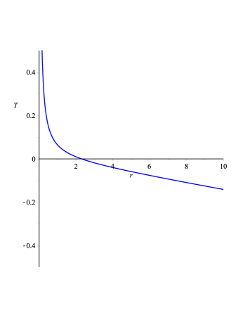
Figure 1: Variation of temprature of the black hole in terms of horizon radius $r_{+}$. $l=4.0$, $\beta_{1}=10^{-4}$.

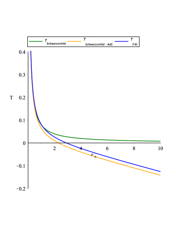
Figure 2: Comparison of variation of temprature in terms of horizon radius $r_{+}$. $l=4.0$, $\beta_{1}=10^{-4}$, for $f(R)$ black hole, $l=4.0$, $\beta_{1}=0$, for Schwarzschild-AdS black hole, and $l=0$, $\beta_{1}=0$, for Schwarzschild black hole.

3.1 Modified thermodynamics due to thermal fluctuations

Exploiting relations (2.7), (3.7) and (3.8), the leading-order corrected entropy due to thermal fluctuations is given by

$$S={\cal S}_{0}-\alpha\log\left[-\frac{4\beta_{1}l^{2}\pi^{1/2}{\cal S}_{0}^{3/2}-6{\cal S}_{0}^{2}+2l^{2}\pi{\cal S}_{0}}{l^{2}\pi+3{\cal S}_{0}}\right]-2\alpha\log\left[\frac{2\beta_{1}l^{2}\pi^{1/2}{\cal S}_{0}^{1/2}-3{\cal S}_{0}+l^{2}\pi}{4\pi^{3/2}l^{2}{\cal S}_{0}^{1/2}}\right].$$ (3.15)

Using standard relation $\left(M=\int T_{H}dS\right)$, the corrected mass is calculated as

$$M = \frac{l^{2}\pi^{1/2}\beta_{1}{\cal S}_{0}+l^{2}\pi{\cal S}_{0}^{1/2}-{\cal S}_{0}^{3/2}}{2l^{2}\pi^{3/2}}+\alpha\frac{l^{2}\pi+3{\cal S}_{0}}{2l^{2}\pi^{3/2}{\cal S}_{0}^{1/2}}+\frac{\sqrt{3}\alpha}{l\pi}\cot^{-1}\left(\frac{l\pi^{1/2}}{\sqrt{3{\cal S}_{0}}}\right)$$ (3.16)

$$- \frac{\alpha\beta_{1}}{4\pi}[3\log{\cal S}_{0}-2\log(l^{2}\pi+3{\cal S}_{0})]-2\alpha\frac{2\beta_{1}l^{2}\pi^{1/2}{\cal S}_{0}^{1/2}-3{\cal S}_{0}+l^{2}\pi}{4\pi^{3/2}l^{2}{\cal S}_{0}^{1/2}}.$$

The corrected heat capacity, using relation $\left(C=T_{H}\frac{\partial S}{\partial T_{H}}\right)$, is computed as

$$C = -\frac{4\beta_{1}l^{2}\pi^{1/2}{\cal S}_{0}^{3/2}-6{\cal S}_{0}^{2}+2l^{2}\pi{\cal S}_{0}}{l^{2}\pi+3{\cal S}_{0}}-2\alpha$$ (3.17)

$$- \alpha\frac{\left(\pi^{2}l^{4}+3\beta_{1}\sqrt{\pi}l^{2}\sqrt{{\cal S}_{0}}\left(\pi l^{2}+{\cal S}_{0}\right)-6\pi l^{2}{\cal S}_{0}-9S^{2}\right)\left(2l^{2}\beta_{1}\sqrt{\pi}{\cal S}_{0}^{3/2}+\pi l^{2}-3{\cal S}_{0}\right)}{{\cal S}_{0}\left(\pi l^{2}+3{\cal S}_{0}\right)\left(2l^{2}\beta_{1}\sqrt{\pi}\sqrt{{\cal S}_{0}}+\pi l^{2}-3{\cal S}_{0}\right)^{2}}.$$

Again, Eqs. (3.16) and (3.17) for $\alpha=0$, and $\beta_{1}=0$, convert to Eqs. (3.9) and (3.11), and for $\alpha=0$, $\beta_{1}=0$ and $\Lambda=0$, convert to Eqs. (3.12) and (3.14), which represent the Schwarzschild-AdS and Schwarzschild black holes, respectively. These thermodynamic parameters are plotted in terms of horizon radius $r_{+}$ (see Figs. 3, 4, 5 and 6).

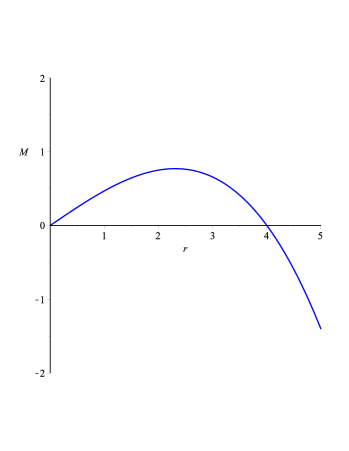
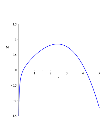
Figure 3: Variation of mass in terms of horizon radius of a static black hole $r_{+}$ for $l=4.0$, $\beta_{1}=10^{-2}$ and $\alpha=0$, $\alpha=0.5$ for (a) and (b), respectively.

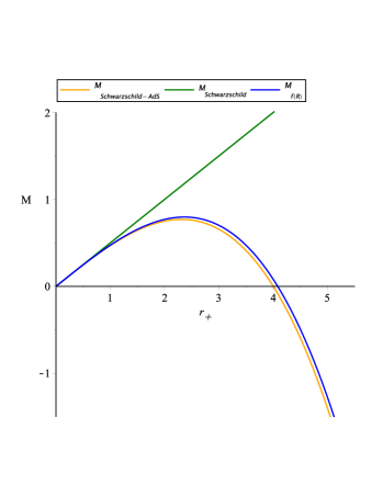
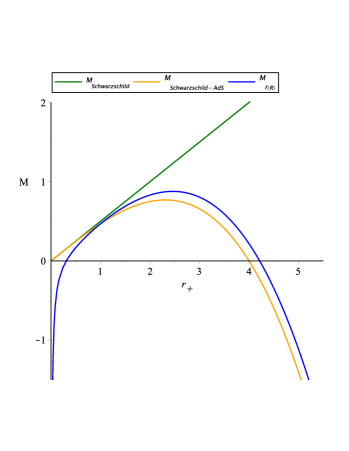
Figure 4: Comparison of variation of mass in terms of horizon radius $r_{+}$. $l=4.0$, $\beta_{1}=10^{-2}$, for $f(R)$ black hole, $l=4.0$, $\beta_{1}=0$, for Schwarzschild-AdS black hole, and $l=0$, $\beta_{1}=0$, for Schwarzschild black hole. Also, $\alpha=0$, $\alpha=0.5$ for (a) and (b), respectively.

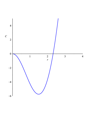
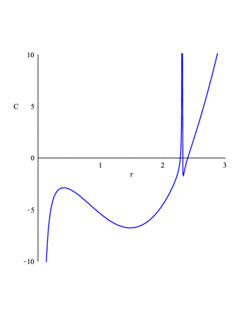
Figure 5: Variation of heat capacity in terms of horizon radius of a static black hole $r_{+}$ for $l=4.0$, $\beta_{1}=10^{-4}$ and $\alpha=0$, $\alpha=0.5$ for (a) and (b), respectively.

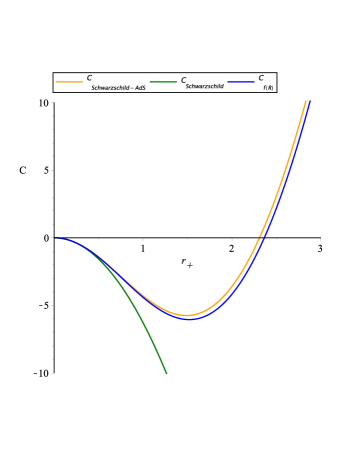
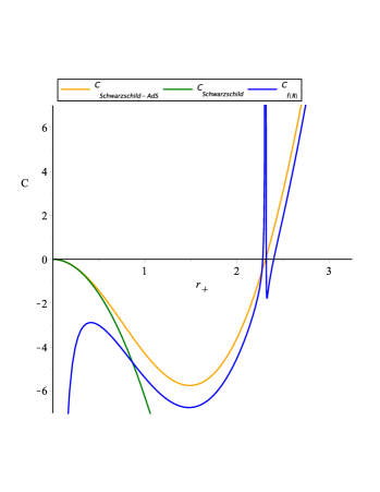
Figure 6: Comparison of variation of heat capacity in terms of horizon radius $r_{+}$. $l=4.0$, $\beta_{1}=10^{-4}$, for $f(R)$ black hole, $l=4.0$, $\beta_{1}=0$, for Schwarzschild-AdS black hole, and $l=0$, $\beta_{1}=0$, for Schwarzschild black hole. Also, $\alpha=0$, $\alpha=0.5$ for (a) and (b), respectively.

From Fig. 3(a), (for $\alpha=0$), it can be seen that, mass of the black hole has a maximum value at $r_{+}=r_{m}=2.31$, and it become zero at two points, $r_{+}=r_{01}=0$ and $r_{+}=r_{02}=4$. Also, as can be seen from Fig. 3(b) (for $\alpha>0$), by increasing $\alpha$, the number of zero points of mass are not changing, but they shift towards larger values.

Moreover, Fig. 4 shows the comparison of variation of mass versus horizon radius for a static black hole in $f(R)$ gravity and the Schwarzschild-AdS and Schwarzschild black holes of standard general relativity. As one can see, for both cases ($\alpha=0$ and $\alpha=0.5$), mass variations are somewhat the same for a static black hole in $f(R)$ gravity and the Schwarzschild-AdS black hole. But for the Schwarzschild black hole the mass variation is quite different.

In addition, plot of the heat capacity can be seen in Fig. 5. In this case, we find that, for the case $\alpha=0$ (Fig. 6(a)), for $0<r_{+}<r_{m}$, the heat capacity is in the negative region (unstable phase), then, at $r_{+}=r_{m}$, it takes type one phase transition, in which $C(r_{+}=r_{m})=0)$, after that, for $r_{+}>r_{m}$, it becomes positive valued (stable). So, for the case $\alpha=0$, this black hole has a type one phase transition. However, (for $\alpha>0$), as can be seen from Fig. 5(b), by increasing $\alpha$, the number of zero points of the heat capacity are changing to the three zero points. In other words, for the case $\alpha=0$, in addition to one zero two other zeroes also appear.

Also, Fig. 6 shows the comparison of variation of the heat capacity versus horizon radius for a static black hole in $f(R)$ gravity and the Schwarzschild-AdS and Schwarzschild black holes of standard general relativity. As we can be seen, for the case $\alpha=0$, the heat capacity variations are somewhat the same for a static black hole in $f(R)$ gravity and the Schwarzschild-AdS black hole. But for the Schwarzschild black hole the heat capacity variation is quite different and it is always in the negative phase and it is unstable. Moreover, for the case $\alpha>0$, these comparisons are somewhat different. For this case, all three black holes have completely different heat capacity variations. the Schwarzschild black hole has no zero and is therefore always unstable. The Schwarzschild-AdS black hole has a zero and therefore, as mentioned earlier, has a phase transition of a type one. The static black hole in $f(R)$ gravity (for $\alpha>0$), has more zeros as alpha increases and therefore has more phase transitions.

3.2 Thermodynamic geometry

In this section, using the geometric technique of Weinhold, Ruppeiner and GTD metrics of the thermal system, we construct the geometric structure for a static black hole in $f(R)$ gravity. In this case, the extensive variables are, $N^{r}=(l,\beta_{1})$. The Weinhold metric is defined as the Hessian in the mass representation as follows [27]

$$g^{W}_{ij}=\partial_{i}\partial_{j}M(S,N^{r}).$$ (3.18)

We can write the Weinhold metric for this system as follows

$$g^{W}_{ij}=\partial_{i}\partial_{j}M(S,l,\beta_{1}).$$ (3.19)

The line element corresponding to Weinhold metric is given by

$$ds^{2}_{W}=M_{SS}dS^{2}+M_{ll}dl^{2}+M_{\beta_{1}\beta_{1}}d\beta_{1}^{2}$$

$$2M_{Sl}dSdl+2M_{S\beta_{1}}dSd\beta_{1}+2M_{l\beta_{1}}dld\beta_{1},$$ (3.20)

therefore

$$g^{W}=\begin{bmatrix}M_{SS}&M_{Sl}&M_{S\beta_{1}}\\ M_{lS}&M_{ll}&M_{l\beta_{1}}\\ M_{\beta_{1}S}&M_{\beta_{1}l}&0\end{bmatrix}.$$ (3.21)

The components of above matrix can be found using the expression of $M$, given in Eq. (3.16). Since the equation of the curvature scalar of the Weinhold metric is too large, so we demonstrate it in Fig. (7).

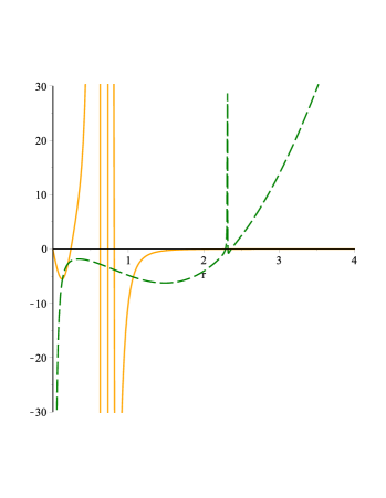
Figure 7: Curvature scalar variation of Weinhold metric (orange continuous line) and the heat capacity of a static black hole (green dash line) in terms of the radius of the horizon r+, for $\alpha=0.5$, $l=4.0$, $\beta_{1}=10^{-4}$.

It can be observed from Fig. 7 that the singular points of curvature scalar of Weinhold metric do not coincide with zero points of heat capacity, so, in this case we can’t find any physical information about the system from the Weinhold method. In following, we use Ruppeiner method, which is conformaly transformed to the Weinhold metric. The Ruppeiner metric is defined by [28, 29, 67]

$$ds^{2}_{R}=\frac{1}{T}ds^{2}_{W}.$$ (3.22)

The matrix corresponding to the metric components of Ruppeiner method is as following:

$$g^{R}=\left(\frac{4l^{2}\pi^{\frac{3}{2}}S_{0}^{\frac{1}{2}}}{2l^{2}\pi^{\frac{1}{2}}S_{0}^{\frac{1}{2}}\beta_{1}-3S_{0}+l^{2}\pi}\right)\begin{bmatrix}M_{SS}&M_{Sl}&M_{S\beta_{1}}\\ M_{lS}&M_{ll}&M_{l\beta_{1}}\\ M_{\beta_{1}S}&M_{\beta_{1}l}&0\end{bmatrix}.$$ (3.23)

Plot of the scalar curvature of the Ruppeiner metric is shown in Fig. 8(a). Also, plots of the curvature scalar of the Ruppeiner metric and the heat capacity, in terms of $r_{+}$, are demonstrated in Fig. 8(b), (c) and (d). As one can see from Fig. 8(b), for the case $\alpha=0$, the heat capacity has only one zero (the phase transition point), however, the singular point of the curvature scalar of Ruppeiner metric completely coincides with zero point of the heat capacity. On the other hand, for the case $\alpha>0$ (see Fig. 8(c), (d)), the heat capacity has three zero points, however, the singular points of the curvature scalar of Ruppeiner metric are not completely coinciding with the zero points of the heat capacity of the static black hole. In fact, only one of the singular point of the curvature scalar of Ruppeiner metric is completely coinciding with one of the zero point of the heat capacity. In the other word, by increasing $\alpha$, this adaptation is reduced.

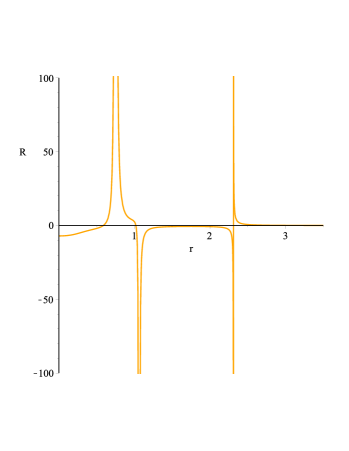
(a) $\alpha=0.5$

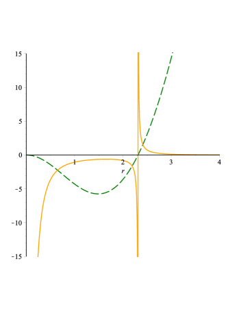
(b) $\alpha=0$

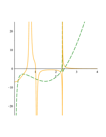
(c) $\alpha=0.5$

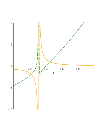
(d) Closeup of figure (c)

Figure 8: Curvature scalar variation of Ruppeiner metric (orange continuous line) and the heat capacity of a static black hole (green dash line) in terms of $r_{+}$ for $l=4.0$, $\beta_{1}=10^{-4}$.

In the next step, we will investigate the GTD method. The general form of the metric in GTD method is as following [31]:

$$g=\left(E^{c}\frac{\partial\Phi}{\partial E^{c}}\right)\left(\eta_{ab}\delta^{bc}\frac{\partial^{2}\Phi}{\partial E^{c}\partial E^{d}}dE^{a}dE^{d}\right),$$ (3.24)

where

$$\frac{\partial\Phi}{\partial E^{c}}=\delta_{cb}I^{b},$$ (3.25)

in which $\Phi$ is the thermodynamic potential, $I^{b}$ and $E^{a}$ are the intensive and extensive thermodynamic variables. So, according to Eq. (3.24), the metric for this thermodynamic system is as following:

$$g^{GTD}=(SM_{S}+lM_{l}+\beta M_{\beta_{1}})\begin{bmatrix}-M_{SS}&0&0\\ 0&M_{ll}&M_{l\beta_{1}}\\ 0&M_{\beta_{1}l}&0\end{bmatrix}.$$ (3.26)

The plot of the scalar curvature of GTD metric is shown in Fig. (9).

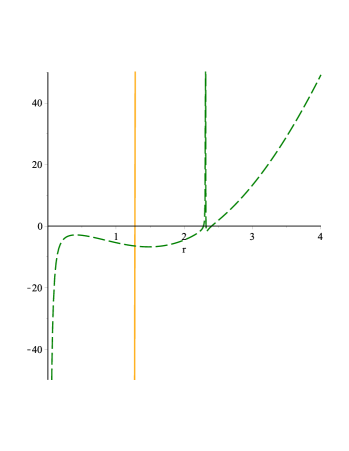
Figure 9: Curvature scalar variation of GTD metric (orange continuous line) and the heat capacity of a static black hole (green dash line) in terms of the radius of the horizon r+, for $\alpha=0.5$, $l=4.0$, $\beta_{1}=10^{-4}$.

It can be observed from Fig. 9, the singular point of curvature scalar of GTD metric does not coincide with zero point of heat capacity, so, in this case we can’t find any physical information about the system from the GTD method.

4 Conclusions

In this paper, we studied small statistical fluctuations around equilibrium for a static black hole in $f(R)$ gravity and analyzed thermodynamic quantities of this black hole according to corrected thermodynamic entropy. We have found that the Hawking temperature is a decreasing function of horizon radius. We have utilized the expressions of Hawking temperature and uncorrected specific heat to evaluate the correction to the entropy of a static black hole in $f(R)$ gravity due to thermal fluctuation. Also, we have computed the first-order corrected mass and heat capacity by utilizing the standard thermodynamical definitions. From graphical study, we observed that the uncorrected mass of the black hole gets a maximum value at $r_{+}=r_{m}=2.31$, and takes zero value at two points, $r_{+}=0$ and $r_{+}=4$. However, for the corrected mass with positive correction coefficient $\alpha$, the number of zero points of mass do not changing, but they appear at larger horizon radius. For the case of heat capacity, we have found that the uncorrected heat capacity has negative values (unstable phase) for $0<r_{+}<r_{m}$ and type one phase transition takes place for black holes undergo at $r_{+}=r_{m}$ as $C(r_{+}=r_{m})=0$. For $r_{+}>r_{m}$, the heat capacity takes positive value (stable). So, one may conclude that without considering thermal fluctuation, this black hole has a type one phase transition. However, due to e thermal fluctuation, the number of zero points of the heat capacity changes to the three zero points.

Also, we investigated the thermodynamic geometry of this black hole and plotted thermodynamic quantities and curvature scalar of Weinhold, Ruppeiner and GTD methods in terms of horizon radius $r_{+}$. We observed that, the singular points of curvature scalar of Weinhold and GTD methods, for both $\alpha=0$ and $\alpha>0$ cases, are not coincided with zero point of heat capacity (the phase transition points). This suggests that we could not find any physical information about the system from these two methods. However, for the case $\alpha=0$, we realized that the heat capacity has only one zero, and the singular point of the curvature scalar of Ruppeiner metric is completely coinciding with it, moreover for the case $\alpha>0$, the heat capacity has three zero points, and the singular points of the curvature scalar of Ruppeiner metric are not completely coinciding with zero points of the heat capacity of this black hole and only one of the singular point of the curvature scalar of Ruppeiner metric is completely coincide with one of the zero point of the heat capacity, that’s mean by increasing $\alpha$, this adaptation is reduced.

References

- [1] J. D. Bekenstein, Phys. Rev. D 7 (1973) 2333.
- [2] S. W. Hawking, Nature 248 (1974) 30.
- [3] P. C. W. Davies, Proc. Roy. Soc. Lond. A 353, 499 (1977).
- [4] S. Hawking and D. N. Page, Commun. Math. Phys. 87, 577 (1983).
- [5] R. G. Cai, L. M. Cao and Y. W. Sun, JHEP 11, 039 (2007).
- [6] D. Kothawala, T. Padmanabhan and S. Sarkar, Phys. Rev. D 78, 104018 (2008).
- [7] Y. S. Myung, Phys. Rev. D 77, 104007 (2008). B. M. N. Carter and I. P. Neupane, Phys. Rev. D 72, 043534 (2005). D. Kastor, S. Ray and J. Traschen, Class. Quant. Grav. 26, 195011 (2009). F. Capela and G. Nardini, Phys. Rev. D 86, 024030 (2012).
- [8] M. Eune, W. Kim and S. H. Yi, JHEP 03, 020 (2013).
- [9] G. Gibbons, R. Kallosh and B. Kol, Phys. Rev. Lett. 77, 4992 (1996).
- [10] B. P. Dolan, Class. Quantum Gravit. 28, 235017 (2011).
- [11] R. Banerjee and D. Roychowdhury, Phys. Rev. D 85, 104043 (2012).
- [12] D. Kubiznak and R. B. Mann, JHEP 07, 033 (2012).
- [13] R. G. Cai, L. M. Cao, L. Li and R. Q. Yang, JHEP 09, 005 (2013).
- [14] M. B. Jahani Poshteh, B. Mirza and Z. Sherkatghanad, Phys. Rev. D 88, 024005 (2013).
- [15] S. Chen, X. Liu and C. Liu, Chin. Phys. Lett. 30, 060401 (2013).
- [16] J. X. Mo and W. B. Liu, Eur. Phys. J. C 74, 2836 (2014).
- [17] D. C. Zou, S. J. Zhang and B. Wang, Phys. Rev. D 89, 044002 (2014).
- [18] W. Xu and L. Zhao, Phys. Lett. B 736, 214 (2014).
- [19] A. M. Frassino, D. Kubiznak, R. B. Mann and F. Simovic, JHEP 09, 214 (2014).
- [20] C. V. Johnson, Class. Quantum Gravit. 31, 205002 (2014).
- [21] B. P. Dolan, JHEP 10, 179 (2014).
- [22] J. Xu, L. M. Cao and Y. P. Hu, Phys. Rev. D 91, 124033 (2015).
- [23] S. H. Hendi, B. Eslam Panah and S. Panahiyan, JHEP 11, 157 (2015).
- [24] A. Mandal, S. Samanta and B. R. Majhi, Phys. Rev. D 94, 064069 (2016).
- [25] S. H. Hendi, R. B. Mann, S. Panahiyan and B. Eslam Panah, Phys. Rev. D 95, 021501(R) (2017).
- [26] R. Hermann, Geometry, physics and systems, (Marcel Dekker., New York, 1973).
- [27] F. Weinhold, J. Chem. Phys 63, 2479 (1975).
- [28] G. Ruppeiner, Phys. Rev. A 20, 1608 (1979).
- [29] P. Salamon, J. D. Nulton and E. Ihrig, J. Chem. Phys, 80,436 (1984).
- [30] G. Ruppeiner, Rev. Mod. Phys. 67, 605 (1995).
- [31] H. Quevedo, J. Math. Phys. 48 (2007) 013506.
- [32] H. Quevedo, Gen. Rel. Grav. 40, 971 (2008).
- [33] A. Strominger, C. Vafa, Phys. Lett. B379 (1996) 99.
- [34] A. Ashtekar, J. Baez, A. Corichi, K. Krasnov, Phys. Rev. Lett. 80 (1998) 905.
- [35] S. Carlip, Phys. Rev. Lett. 82 (1999) 2828.
- [36] S. N. Solodukhin, Phys. Lett. B454 (1999) 213.
- [37] A. Ashtekar, Lectures on Non-perturbative Canonical Gravity, World Scientific (1991).
- [38] S. Das, P. Majumdar, R. K. Bhaduri, Class. Quant. Grav.19:2355-2368, (2002).
- [39] A. Pathak, A. P. Porfyriadis, A. Strominger and O. Varela, JHEP 04 (2017) 090.
- [40] S. Carlip, Class. Quant. Grav. 17, 4175 (2000).
- [41] S. Upadhyay and B. Pourhassan, Prog. Theor. Exp. Phys. 013B03 (2019).
- [42] S. Upadhyay, Phys. Lett. B 775, 130 (2017).
- [43] B. Pourhassan, M. Faizal, S. Upadhyay and L. A. Asfar, Eur. Phys. J. C 77, 555 (2017).
- [44] B. Pourhassan, S. Upadhyay and H. Farahani, Int. J. Mod. Phys. A 34 (2019) 1950158.
- [45] N.-ul Islam, P. A. Ganai, S. Upadhyay, Prog. Theor. Exp. Phys. 103B06 (2019).
- [46] S. Upadhyay, Gen. Rel. Grav. 50, 128 (2018).
- [47] A. Pourdarvish, J. Sadeghi, H. Farahani and B. Pourhassan, Int. J. Theor. Phys. 52, 3560 (2013).
- [48] S. Upadhyay, B. Pourhassan and H. Farahani, Phys. Rev. D 95, 106014 (2017).
- [49] B. Pourhassan, S. Upadhyay, H. Saadat and H. Farahani, Nucl. Phys. B 928 (2018) 415.
- [50] B. Pourhassan, M. Faizal, and U. Debnath, Eur. Phys. J. C 76, 145 (2016). York, 1973).
- [51] C. Brans and R. H. Dicke, Phys. Rev. 124, 925 (1961).
- [52] A. G. Riess et al. [Supernova Search Team Collaboration], Astron. J. 116, 1009 (1998). S. Perlmutter et al. [Supernova Cosmology Project Collaboration], Astrophys. J. 517, 565 (1999). J. L. Tonry et al. [Supernova Search Team Collaboration], Astrophys. J. 594, 1 (2003). C. L. Bennett et al. [WMAP Collaboration], Astrophys. J. Suppl. 148, 1 (2003). G. Hinshaw et al. [WMAP Collaboration], Astrophys. J. Suppl. 170, 288 (2007).
- [53] Y. Fujii and K. Maeda. The Scalar-Tensor Theory of Gravitation (Cambridge University Press, Cambridge, 2003). T. P. Sotiriou, Class. Quant. Grav. 23, 5117 (2006).
- [54] P. Brax and C. van de Bruck, Class. Quant. Grav. 20, R201 (2003). L. A. Gergely, Phys. Rev. D 74, 024002 (2006). M. Demetrian, Gen. Rel. Grav. 38, 953 (2006).
- [55] H. A. Buchdahl, Mon. Not. Roy. Astron. Soc. 150, 1 (1970).
- [56] A. A. Starobinsky, Phys. Lett. B 91, 99 (1980).
- [57] K. Bamba and S. D. Odintsov, JCAP 0804, 024 (2008).
- [58] S. Soroushfar, R. Saffari, S. Kazempour, S. Grunau and J. Kunz, Phys. Rev. D 94, 024052 (2016).
- [59] S. Dastan, R. Saffari and S. Soroushfar, arXiv:1606.06994 [gr-qc].
- [60] S. Chakraborty and S. SenGupta, Eur. Phys. J. C 75,538 (2015).
- [61] A. Bohr and B. R. Mottelson, “Nuclear Structure”, Vol.1 (W. A. Benjamin Inc., New York, 1969).
- [62] R. K. Bhaduri, “Models of the Nucleon”, (Addison-Wesley, 1988).
- [63] R. Saffari and S. Rahvar, Phys. Rev. D 77, 104028 (2008).
- [64] S. Soroushfar, R. Saffari, J. Kunz and C. Lämmerzahl, Phys. Rev. D 92, 044010 (2015).
- [65] R. Tharanath, J. Suresh, N. Varghese and V. C. Kuriakose, Gen. Rel. Grav. 46, 1743 (2014).
- [66] S. Soroushfar, R. Saffari and N. Kamvar, Eur. Phys. J. C 76, 476 (2016).
- [67] R. Mrugala, Physica. A (Amsterdam), 125, 631 (1984).