Phase space reconstruction for non-uniformly sampled noisy time series

Abstract

Analyzing data from paleoclimate archives such as tree rings or lake sediments offers the opportunity of inferring information on past climate variability. Often, such data sets are univariate and a proper reconstruction of the system’s higher-dimensional phase space can be crucial for further analyses. In this study, we systematically compare the methods of time delay embedding and differential embedding for phase space reconstruction. Differential embedding relates the system’s higher-dimensional coordinates to the derivatives of the measured time series. For implementation, this requires robust and efficient algorithms to estimate derivatives from noisy and possibly non-uniformly sampled data. For this purpose, we consider several approaches: (i) central differences adapted to irregular sampling, (ii) a generalized version of discrete Legendre coordinates and (iii) the concept of Moving Taylor Bayesian Regression. We evaluate the performance of differential and time delay embedding by studying two paradigmatic model systems – the Lorenz and the Rössler system. More precisely, we compare geometric properties of the reconstructed attractors to those of the original attractors by applying recurrence network analysis. Finally, we demonstrate the potential and the limitations of using the different phase space reconstruction methods in combination with windowed recurrence network analysis for inferring information about past climate variability. This is done by analyzing two well-studied paleoclimate data sets from Ecuador and Mexico. We find that studying the robustness of the results when varying the analysis parameters is an unavoidable step in order to make well-grounded statements on climate variability and to judge whether a data set is suitable for this kind of analysis.

Nonlinear methods such as recurrence quantification analysis and recurrence network analysis offer the prospect of gaining valuable insights into past climate variability. In order to apply these methods, the phase space of the underlying dynamical system has to be reconstructed if the system dynamics are expected to be higher-dimensional than the measured data. In the paleoclimate context, observations are usually univariate while the dynamics of the climate system cannot be assumed to be low-dimensional. Additionally, time series of paleoclimate proxies are often non-uniformly sampled and subject to noise, giving rise to challenges for phase space reconstruction and raising the question how reliable results are when applying nonlinear methods. By systematically studying different phase space reconstruction techniques and combining them with windowed recurrence network analysis, we want to address this problem. We find that not all data sets are suited for recurrence network analysis and that the robustness of the results has to be studied before drawing conclusions about past climate variability.

I Introduction

Reconstructing a system’s phase space from measured data is a standard procedure in nonlinear time series analysis. In particular, finding a proper embedding is a key step in many applications. Among others, recurrence-based methods often make use of embedded time series and have been proven useful in studying dynamical transitions in a variety of disciplines, ranging from medical to paleoclimate data Marwan et al. (2007); Donges et al. (2011a). For example, when aiming at detecting and characterizing nonlinear regime shifts in past climate variability by analyzing data from paleoclimate archives such as tree rings, lake sediments or speleothems, the reconstruction of the system’s higher-dimensional phase space is unavoidable. This is, because the dynamics of the climate system are not expected to be low-dimensional but the measured time series are commonly univariate. Also, proxy variables can be assumed to have been influenced by more than one climate variable. Since such data are inherently subject to noise and very often non-uniformly sampled, methodological difficulties arise. For example, time delay embedding is not well defined for non-uniformly sampled data. Moreover, common approaches to estimate appropriate embedding parameters rely on regularly sampled time series Rehfeld et al. (2011). Still, such kind of analyses constitute an important step towards better understanding the climate of the past. This is not only a historically relevant task but can also serve to assess major implications for modern civilizations in the context of recent climate change. It has been shown that climate variability and extremes can trigger migration Donges et al. (2015a), armed conflict Schleussner et al. (2016) and the development of civilization Donges et al. (2015a), the most prominent example being the rise and fall of the Classic Maya Culture Kennett et al. (2012); Carleton, Campbell, and Collard (2017).

To gain additional insights into the underlying dynamical principles of the climate system, a reliable analysis framework is required. We here aim at contributing to the further development of such a framework by systematically studying different methods to reconstruct the phase space of a system from a measured univariate time series that may be non-uniformly sampled and subject to noise. In particular, we study how those different phase space reconstructions behave when combining them with windowed recurrence network analysis. To do so, we compare the method of time delay embedding with that of differential embedding and present several approaches of estimating derivatives from noisy, non-uniformly sampled data in Sec. II. We then reconstruct the phase space of two paradigmatic model systems and compare their geometric properties to those of the original attractors using recurrence network analysis in Sec. III. Finally, we apply the different phase space reconstruction methods in combination with windowed recurrence network analysis to two well-studied real-world paleoclimate data sets and test the robustness of this analysis framework when varying the different analysis parameters in Sec. IV. We summarize our insights and conclusions in Sec. V.

II Methods

II.1 Phase space reconstruction

Attractors of dynamical systems can be reconstructed topologically equivalent from data as has been shown in the embedding theorems by Whitney Whitney (1936), Takens Takens (1980) and Mañé Mañé (1981). Takens and Packard independently suggested differential embedding and time delay embedding as two methods to reconstruct the higher-dimensional phase space of a system from a measured, univariate time series Takens (1980); Packard et al. (1980).

Time delay embedding substitutes the non-observed essential coordinates of the system by delayed versions of the measured time series, i. e., if the time series $x(t_{i})$ was measured at times $t_{i},i=1,\dots,N$, the reconstructed state vectors are given by

$$x(t_{i})\rightarrow\left\{x(t_{i}),x(t_{i}-\tau),\dots,x(t_{i}-(m-1)\tau)\right\}$$ (1)

with $\tau$ some suitable time delay and $m$ the embedding dimension. In a similar way, differential embedding relates the higher-dimensional coordinates to the respective derivatives up to order $m-1$,

$$x(t_{i})\rightarrow\left\{x(t_{i}),\dfrac{dx(t_{i})}{dt},\dots,\dfrac{d^{m-1}x(t_{i})}{dt^{m-1}}\right\}.$$ (2)

Takens proved that for regularly sampled and noise free data, the attractors reconstructed using time delay or differential embedding are diffeomorphic to the original attractor if the embedding dimension is larger than twice the dimension of the original attractor Takens (1980). The work of Packard et al. Packard et al. (1980) was more practically inspired, searching for independent coordinate representations from experimental data and suggesting both the method of delays and the method of derivatives.

Since then, much work has focused on how to choose the delay time and embedding dimension for given data. Practically, the dimension of the system’s attractor is not known and any measurement process will be subject to noise. For noise-free data, any delay time $\tau$ can be chosen, whereas in the presence of noise the choice of the embedding delay can be crucial (Casdagli et al., 1991). The first zero of the autocorrelation or the first minimum of the mutual information have been suggested as practically applicable criteria Kantz and Schreiber (2004); Abarbanel et al. (1993); Fraser and Swinney (1986). To deal with noise, principal component embedding has been developed Gibson et al. (1992); Casdagli et al. (1991). For the embedding dimension, the false nearest neighbor algorithm has been shown to provide a reasonable estimate Kennel, Brown, and Abarbanel (1992). A recent approach avoids the choice of dimension by using an infinite dimensional embedding with weighted coordinates, introducing a scaling factor Hirata and Aihara (2017).

The above discussion shows that the choice of embedding parameters is a subject of ongoing research. In this context, the problem of non-uniform sampling of the data has not yet been addressed sufficiently. In this case, time delay embedding suffers from conceptual problems. Not only standard estimators for the autocorrelation and mutual information rely on regularly sampled time series Ozken et al. (2015); Rehfeld et al. (2011); Rehfeld and Kurths (2014), also the embedding itself is not well defined for irregular sampling such that interpolation of the data becomes unavoidable. In turn, differential embedding does not suffer from those conceptual problems and the choice of derivatives as higher-dimensional coordinates may seem more natural than that of delays, in particular, when thinking of the dynamics of a system to be generated by differential equations. In addition, it obeys only one characteristic parameter ($m$) instead of two ($m$, $\tau$), which may be beneficial in real-world cases. However, differential embedding has not yet been used often in practice as the robust numerical estimation of derivatives from noisy data is challenging.

II.2 Estimating derivatives

In the following, we discuss different techniques to estimate derivatives from noisy and possibly non-uniformly sampled data. That is, given a time series $x_{i}=x(t_{i})$ for $i=1,\dots,N$ and non-uniform sampling intervals $\Delta t_{i}=t_{i+1}-t_{i}$, we want to approximate the time derivatives

$$\frac{d^{j}x}{dt^{j}}\bigg{|}_{t=t_{i}} \equiv\frac{d^{j}}{dt^{j}}x_{i}$$ (3)

at all times $t_{i}$ and for orders $j$ up to some order $j_{\max}$.

II.2.1 Central differences

The first and probably simplest approach to numerically estimate derivatives is to approximate the derivative by differences. For regular sampling the central difference quotient is given as

$$\frac{d}{dt}x_{i}\approx\frac{\Delta x_{i}}{\Delta t} =\dfrac{x_{i+1}-x_{i-1}}{2\Delta t}.$$ (4)

Taking non-uniform sampling into account, this formula can be generalized to

$$\frac{\Delta x_{i}}{\Delta t}=\dfrac{\Delta t_{i-1}^{2}x_{i+1}-(\Delta t_{i-1}^{2}-\Delta t_{i}^{2})x_{i}-\Delta t_{i}^{2}x_{i-1}}{\Delta t_{i-1}\Delta t_{i}(\Delta t_{i-1}+\Delta t_{i})},$$ (5)

which reduces to (4) when $\Delta t_{i}=\Delta t_{i-1}$. To derive the above expression, we approximate the values of the neighboring points of our target point $x_{i}$ using a Taylor expansion up to second order:

$$x_{i-1} \approx x_{i}-\Delta t_{i-1}\frac{d}{dt}x_{i}+\dfrac{\Delta t_{i-1}^{2}}{2}\frac{d^{2}}{dt^{2}}x_{i},$$

$$x_{i+1} \approx x_{i}+\Delta t_{i}\frac{d}{dt}x_{i}+\dfrac{\Delta t_{i}^{2}}{2}\frac{d^{2}}{dt^{2}}x_{i}.$$

Eliminating the term with the second derivatives from this system of equations and solving for $\frac{d}{dt}x_{i}$ gives the desired result (5). Higher order derivatives can be obtained by repeatedly applying Eq. (5).

II.2.2 Discrete Legendre polynomials

A refined approach to estimate derivatives suggested by Gibson et al. Gibson et al. (1992) uses discrete Legendre polynomials. This concept can be generalized to irregular sampling and relates the $j$th derivative at $x_{i}$ to a weighted sum of the $p$ nearest points to each side of $x_{i}$ as

$$\dfrac{d^{j}}{dt^{j}}x_{i} \approx\dfrac{j!}{c_{j,p}(\Delta t_{i,n})}\sum_{n=-p}^{p}r_{j,p,n}^{(i)}x_{i+n}$$ (6)

with $\Delta t_{i,n}=t_{i+n}-t_{i}$ and

$$c_{j,p}(\Delta t_{i,n}) =\sum_{n=-p}^{p}(\Delta t_{i,n})^{j}r_{j,p,n}^{(i)}.$$

The weights are given by the discrete Legendre polynomials $r_{j,p,n}^{(i)}=r_{j,p}(\Delta t_{i,n})$ that can be calculated recursively by the relation

$$r_{j,p,n}^{(i)} =\dfrac{1}{c_{j}p^{j}}\left[\Delta t_{i,n}^{j}-\sum_{k=0}^{j-1}r_{k,p,n}^{(i)}\sum_{l=-p}^{p}\Delta t_{i,l}^{j}r_{k,p,l}^{(i)}\right]$$ (7)

for $2p\geq j$ with $r_{0,p,n}^{(i)}=1/c_{0}$. The normalization constants $c_{j}$ can be determined by the conditions

$$\sum_{n=-p}^{p}(r_{j,p,n}^{(i)})^{2} =1.$$ (8)

The derivation of (6) can be found in the appendix A. It should be noted that the discrete Legendre polynomials are not a discretization of the common Legendre polynomials. Instead, for $p\rightarrow\infty$, they converge to the latter. By changing the parameter $p$ (the number of neighbors to each side that are included for estimating the derivatives) it is possible to control the smoothing of the data. That is, some noise can be averaged out which makes this procedure more robust with respect to noise than other methods. For estimating the optimal value of $p$, a procedure has been suggested by Gibson et al.Gibson et al. (1992). In general, we recommend choosing a $p$ of the order of the embedding dimension, i. e. of the order of the highest derivative that needs to be estimated. In the limit case of choosing $p$ as small as possible, this approach reduces to a central difference quotient.

II.2.3 Moving Taylor Bayesian Regression

The concept of Moving Taylor Bayesian Regression (MoTaBaR) introduced by Heitzig Heitzig (2013) can be used to estimate the value of some function $f$ and its derivatives of order smaller than $p$ at some specific position of interest $\xi$. To do so, a set of $N$ measured data points, prior beliefs about the variability of argument and measurement error and about the variability of $f$ and some of its derivatives are required. In the context of paleoclimate data, the argument and measurement errors correspond to the time and measurement uncertainties. Using the measured data and Bayesian updating, posterior distributions can be obtained from the prior distributions and the posterior mean and variance can be used as estimators of the value and uncertainty of the function and its derivatives at $\xi$. To be more precise, we here assume that the measured data set $\left\{x_{i},y_{i}\right\}_{i=1}^{N}$ is one-dimensional, that the argument and measurement errors ($\gamma_{i}$ and $\epsilon_{i}$) are Gaussian and that we do not have prior information about the variability of the function $f$ and its derivatives. A local Taylor approximation at the position of interest $\xi$ relates the measured values to the derivatives $\varphi^{\alpha}=\frac{d^{\alpha}f(\xi)}{dx^{\alpha}}$ as

$$y_{i} =\sum_{\alpha=0}^{p-1}X_{i,\alpha}\varphi^{\alpha}+r_{i}+\epsilon_{i}.$$

The $X_{i,\alpha}$ are given by

$$X_{i,\alpha} =\dfrac{(x_{i}-\gamma_{i}-\xi)^{\alpha}}{\alpha!}$$ (9)

and $r_{i}$ is the Taylor residual

$$r_{i} =X_{i,p}\psi_{i},$$

$$\psi_{i} =\dfrac{d^{p}}{dx^{p}}f(\xi+\lambda_{i}(x_{i}-\gamma_{i}-\xi))$$

with $\lambda_{i}\in[0,1]$. The procedure to estimate the posterior mean $\tilde{\mu}_{\varphi}$ and variance $\tilde{\Sigma}_{\varphi}$ of $f$ and its derivatives for non-informative priors, i. e.  prior variance $\Sigma_{\varphi}^{-1}=0$ and prior mean of $\psi$, $\mu_{\psi}=0$, is as follows:

• Calculate $X_{i,\alpha}$ for all $i$ and $\alpha<p$ from $x$, $\gamma$ and $\xi$ using (9).

• Calculate $\left(\Sigma_{r}\right)_{i,j}$ from the prior belief about $\left(\Sigma_{\psi}\right)_{i,j}$

  $$\left(\Sigma_{r}\right)_{i,j} =X_{i,p}\left(\Sigma_{\psi}\right)_{i,j}X_{j,p}.$$

• Calculate $W=(\Sigma_{r}+\Sigma_{\epsilon})^{-1}$.

• Obtain the posterior variance and mean as

  $$\tilde{\Sigma}_{\varphi} =(X^{\prime}WX)$$

  $$\tilde{\mu}_{\varphi} =\tilde{\Sigma}_{\varphi}(X^{\prime}Wy).$$

If the distribution of the argument errors $\rho(\gamma|x)$ is known, the final estimators $\hat{\varphi}$ and $\hat{\Sigma}_{\varphi}$ can be obtained by integrating over all possible argument errors. A detailed and more general description of the method can be found in Heitzig (2013).

II.3 Recurrence network analysis

Recurrences in phase space have been successfully used for characterizing system dynamics in many fields of application Marwan et al. (2007). The underlying concept of recurrence plots relies on the recurrence matrix $R_{i,j}$

$$R_{i,j}(\epsilon) =\theta\left(\epsilon-\|\vec{x}_{i}-\vec{x}_{j}\|\right)$$ (10)

that quantifies at which points $t_{j}$ in time the observed trajectory of the system is closer to some previous state $\vec{x}_{i}=\vec{x}(t_{i})$ than a given threshold distance $\epsilon$ with respect to some metric $\|\cdot\|$ in phase space. Here, $\theta(\cdot)$ is the Heaviside function and $\vec{x}_{i}$ is the state vector of the system at time $t_{i}$. To quantify distances, we use the supremum norm

$$\|\vec{z}\|_{\infty} =\max_{j=1,\dots,m}\left\{z^{(j)}\right\}$$

with $m$ the dimension of the time series.

Beyond the characterization of recurrences in phase space, time series analysis using complex network techniques has received considerable attention in the past few years. Different classes of networks have been suggested to characterize the dynamics of a system from a time series Donner et al. (2010a, 2011a). Among these different concepts, recurrence networks integrate the two aspects of recurrences and time series analysis using complex networks by reinterpreting the recurrence matrix as the adjacency matrix of a complex network as

$$A_{i,j}(\epsilon) =R_{i,j}(\epsilon)-\delta_{i,j},$$ (11)

where the delta function $\delta_{i,j}$ excludes self-connections. That is, the nodes of the recurrence network correspond to the state vectors of the system under study that can be identified with a certain time of observation. A link between two nodes is established when the states are closer than the threshold $\epsilon$ in phase space.

It should be noted that recurrence network analysis solely captures geometric properties of the system in phase space and is invariant under re-ordering of the nodes. Specifically, the network structure depends on the geometric characteristics of the system’s attractor and can be characterized using measures like the average path length $\mathcal{L}$ and network transitivity $\mathcal{T}$ Donner et al. (2010b, 2011b). This makes recurrence network analysis particularly suitable for comparing different attractor reconstructions in phase space. The average path length is defined as

$$\mathcal{L} =\dfrac{2}{N(N-1)}\sum_{i<j}l_{i,j}$$ (12)

with $l_{i,j}$ denoting the length of the shortest path between node $i$ and node $j$. Low average path lengths have been attributed to more regular dynamics of the system while high values indicate more chaotic dynamics Donner et al. (2010b). The network transitivity is defined as

$$\mathcal{T} =\dfrac{\sum_{v,i,j}A_{v,i}A_{i,j}A_{j,v}}{\sum_{v,i,j}A_{v,i}A_{j,v}},$$ (13)

which can be interpreted as the probability that two neighbors $i$ and $j$ of a randomly chosen node $v$ in the network are mutually connected. High values of the transitivity correspond to lower-dimensional dynamics while low values relate to higher-dimensional dynamics Donner et al. (2010b). In this context, transitivity has been demonstrated to constitute a generalized notion of dimensionality of a chaotic attractor Donner et al. (2011b).

III Model systems

To study the potential of the different ways to reconstruct the phase space of a system from noisy and non-uniformly sampled data, we first consider two model systems, the Lorenz Lorenz (1963) and the Rössler system Rössler (1976), which are given as

$$\dot{x} =a(y-x)$$

$$\dot{y} =x(b-z)-y$$

$$\dot{z} =xy-cz$$

and

$$\dot{x} =-y-z$$

$$\dot{y} =x+dy$$

$$\dot{z} =e+z(x-f),$$

respectively. To obtain a high-resolution reference solution, we numerically integrate the respective set of differential equations with a high sampling rate ($dt=0.001$) with regular sampling. As parameters and initial conditions, we chose $a=10,b=28,c=8/3$, $x_{0}=-8.0,y_{0}=8.0,z_{0}=27.0$ for the Lorenz and $d=0.15$, $e=0.2$, $f=10.$, $x_{0}=0.5$, $y_{0}=0.0$, $z_{0}=0.0$ for the Rössler system. These choices of parameters correspond to the canonical choices that lead to chaotic solutions.

III.1 Analysis procedure

The basic idea is to compare some characteristics of recurrence networks constructed from the reference attractors and using different phase space reconstructions. To do so, we first construct non-uniformly sampled and noisy time series from the reference series. This is done in a two-step procedure. First, we randomly draw $N-1$ time intervals from a gamma distribution

$$P_{\Gamma}(t) =t^{k-1}\dfrac{\exp(-t/\theta)}{\theta^{k}\Gamma(k)}$$ (14)

where $\theta$ is the scale and $k$ is the shape parameter of the distribution. By using the corresponding values of the $x$-coordinate of the respective model system at the resulting times, we end up with a non-uniformly sampled time series of length $N$. Specifically, we employ $500$ independent random permutations of the gamma distributed sampling intervals to obtain $500$ different realizations of the non-uniformly sampled time series.

In a second step, we add white noise to the data

$$x_{i} \rightarrow x_{i}+\eta_{i}$$

where the noise $\eta$ is chosen according to a normal distribution

$$p(x) =\dfrac{1}{\sqrt{2\pi\sigma^{2}}}{\rm e}^{-\frac{(x-\mu)^{2}}{2\sigma^{2}}}$$ (15)

with mean $\mu$ and variance $\sigma^{2}$. The resulting time series exhibits some typical characteristics of measured time series and is then used to reconstruct the systems’ attractors in phase space using time delay embedding on the one hand and differential embedding with different methods to estimate the derivatives on the other hand. Note that the effect of noise on attractor reconstructions from regularly sampled time series has already been studied elsewhere Xiang et al. (2012); Jacob et al. (2016).

As time delay embedding requires regular sampling, we first interpolate the data back to regular sampling using either linear or cubic spline interpolation. For differential embedding, we directly use the non-uniformly sampled data. Additionally, we consider the two interpolated data sets and also compare the situations with and without scaling each coordinate of the embedded data to unit variance. Note that for time delay embedding, the variance of all reconstructed coordinates is by definition of the same order while for differential embedding this is not necessarily the case. The scaling to unit variance accounts for that fact.

From each embedded time series, we finally construct recurrence networks and calculate network transitivity $\mathcal{T}$ and average path length $\mathcal{L}$ to characterize the attractors. We also calculate the corresponding network measures for regular reference solutions $(x,y,z)$ of equal length $N$ and denote them as $\mathcal{T}_{\text{ref}}$ and $\mathcal{L}_{\text{ref}}$, respectively. This is done by subsampling the original high resolution time series according to the average sampling time of the lower resolution non-uniformly sampled time series. To quantify the quality of the attractor reconstruction, we use the mean and standard deviation of the relative difference of the network measures between the reference and the reconstructed attractor

$$\Delta\mathcal{T} =\dfrac{\lvert\mathcal{T}_{\text{ref}}-\mathcal{T}\rvert}{\mathcal{T}_{\text{ref}}},\qquad\Delta\mathcal{L}=\dfrac{\lvert\mathcal{L}_{\text{ref}}-\mathcal{L}\rvert}{\mathcal{L}_{\text{ref}}}$$

taken over all $500$ realizations of the non-uniform sampling.

III.2 Results

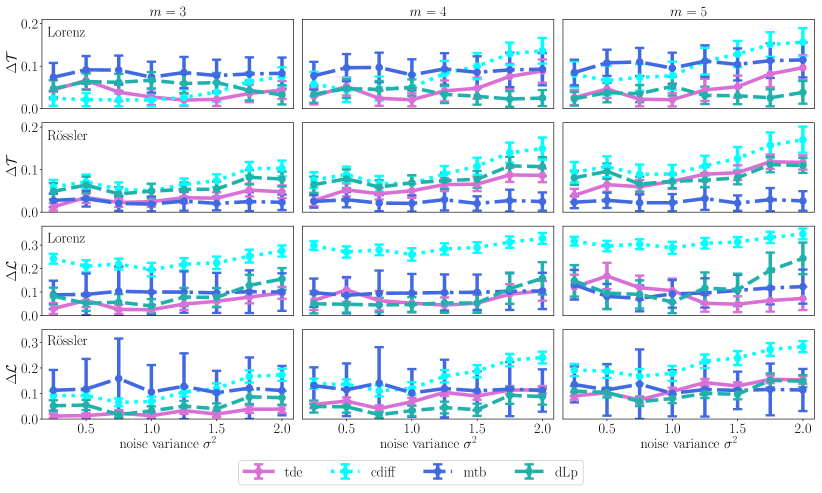
Figure 1: Mean and standard deviation of $\Delta\mathcal{T}$ and $\Delta\mathcal{L}$ as a function of the noise variance $\sigma^{2}$ for the Lorenz and the Rössler system and increasing embedding dimension for different attractor reconstructions. Purple solid lines: time delay embedding (tde) for $\tau=2\left\langle\Delta t\right\rangle$ (Lorenz) and $\tau=\left\langle\Delta t\right\rangle$ (Rössler) and linear interpolation. Light blue dotted lines: central differences (cdiff) scaled to unit variance for cubic spline interpolation. Dark blue dash-dotted lines: MoTaBaR (mtb) based derivative estimates scaled to unit variance and internally interpolated. Cyan dashed lines: discrete Legendre polynomials (dLp) for $p=4$ ($m=3$) and $p=6$ ($m=4,5$) for cubic spline interpolation scaled to unit variance (Lorenz) and without scaling (Rössler).

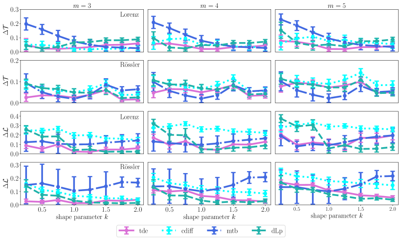
Figure 2: Same as in Fig. 1 for the dependence on the shape parameter $k$ of the sampling interval distribution.

We now study how well the different attractor reconstruction techniques perform when varying (i) the noise level and (ii) the shape parameter of the gamma distribution that determines the non-uniform sampling. For this, we sample ensembles of $N=500$ points each from the reference solutions as described in the previous section. The sampling intervals are distributed according to the gamma distribution (14) with scale parameter $\theta=8.0$ and varying shape parameter $k\in[0.25,2.0]$. The additive noise is given by Eq. (15) with mean $\mu=0$ and variance $\sigma^{2}$ varying in the interval $[0.25,2.0]$.

For time delay embedding, we chose the linearly interpolated data and a delay time of $\tau=\left\langle\Delta t\right\rangle$ for the Rössler and of $\tau=2\left\langle\Delta t\right\rangle$ for the Lorenz system with $\left\langle\Delta t\right\rangle$ being the corresponding average sampling time. This choice of delay times is motivated by calculating the autocorrelation of the time series as a function of the delay and choosing the first zero as delay time $\tau$ Kantz and Schreiber (2004). Also, we found that these choices of the delay time correspond to those that give the best results for the attractor reconstruction. We chose linear interpolation as this is the most commonly used technique when reconstructing the phase space of a system from non-uniformly sampled data using time delay embedding.

For differential embedding using central differences, a procedure first interpolating the data to regular sampling via cubic splines and then rescaling the coordinates to unit variance was found to perform best. For MoTaBaR, we focus on the derivative estimates that were interpolated to regular sampling using the internal MoTaBaR interpolation routine and including $N_{mtb}=20$ data points to estimate the derivatives. Here, the data were again scaled to unit variance. Finally, for the discrete Legendre polynomials, we also found the best results for cubic spline interpolation. For the Lorenz system, additionally rescaling the data to unit variance greatly improved the results while for the Rössler system, the results were best without rescaling. A possible reason for this is that the Rössler system exhibits one outstanding coordinate ($z$) with values of a different order of magnitude than the other coordinates. As the number of neighboring points that are included to each side when estimating the derivatives, we chose $p=4$ for embedding dimension $m=3$ and $p=6$ for $m=4$ and $m=5$. As already mentioned, the choice of $p$ can be justified using a recursive algorithm proposed in Gibson et al. (1992). In our case this suggests $p$ of the order $3$. As this estimation procedure is independent of the embedding dimension and we require estimates of higher order derivatives, we prefer to choose $p$ accordingly a bit higher. Another approach to estimate a reasonable value for $p$ for oscillating data is to choose $p$ such, that the points taken into account to both sides together cover approximately a quarter of an oscillation Gibson et al. (1992). For very noisy data, applying this approach can however be difficult in practice as identifying the system’s oscillations from noisy data can be challenging. For the model systems considered here, the latter method would result in a choice of $p$ around $6$. Our choice of $p$ is thus in accordance with the above considerations. Also, we find that those choices perform quite well compared to other values of $p$. In particular, we find that for lower/higher embedding dimensions a slightly lower/higher choice of $p$ performs better (not shown).

When increasing the noise level (Fig. 1), we expect the results to gradually get worse. Also, for higher embedding dimensions and differential embedding, the noise effect should amplify as higher-order derivatives need to be estimated which are more sensitive to noise. For time delay embedding, this trend is visible in most cases. Still, this approach performs quite well for high noise levels, in particular for the difference of the average path length in the case of $m=3$ and in the case of $m=6$ for the Lorenz system. Also for differential embedding using central differences, the reconstructions tend to differ more from the reference attractor for higher noise level. However, this method generally performs worse than the other methods. For differential embedding using MoTaBaR, we observe a relatively constant difference to the reference attractors’ properties but a higher standard deviation among the $500$ different realizations. This method performs particularly well compared to the other approaches for the difference in transitivity and the Rössler system. Also, MoTaBaR in conjunction with irregular sampling and using the internal interpolation shows in all cases a very similar behavior, though the interpolated case always gives slightly better results (not shown). When using differential embedding with discrete Legendre polynomials, we sometimes observe the expected increase of the difference to the reference case when increasing the noise level. However, in other cases, the results hardly depend on the noise level, in particular for the difference in transitivity for the Lorenz system and also up to a high noise level for the difference in average path length for the Rössler system.

When changing the shape parameter $k$ of the gamma distribution (Fig. 2), we expect better performance for higher values of the parameter as in this case, the distribution is more centered and thus closer to regular sampling. For time delay embedding, this expected trend is visible in some cases but not in all. Still, it performs relatively good for most cases. Differential embedding using central differences for derivative estimation provides rather constant results when varying the shape parameter of the gamma distribution. But, except for the difference to the transitivity of the Lorenz system where it exhibits reasonable results for small values of the shape parameter, this approach does not perform very well compared to the other methods. Differential embedding using MoTaBaR derivative estimates shows the expected trend very clearly for the difference to the reference transitivity. For the difference in the average path length, it first improves performance with increasing the shape parameter, then, when further increasing it, the performance gets worse again. For differential embedding using discrete Legendre polynomials to estimate the derivatives, we mostly find the expected trend and particularly notice a large difference in performance for the average path length in the Lorenz system between $k=0.75$ and $k=1.0$.

Overall, we have found that time delay embedding using linear interpolation performs quite well but often differential embedding using discrete Legendre polynomials or MoTaBaR performs even better. In contrast to this, differential embedding with estimating the derivatives by central differences does not perform very well in almost all cases. Hence, we conclude that more sophisticated methods should be applied to estimate derivatives from noisy and non-uniformly sampled data. Also, we have found that in general, the recurrence network transitivity is slightly closer to the reference transitivity than the average path length to its reference.

IV Application to paleoclimate data sets

We will now apply the different phase space reconstruction methods in combination with recurrence network analysis to two well-studied paleoclimate time series from Ecuador and Mexico. The aim is to detect nonlinear regime shifts in past climate variability. To do so, we will first introduce the proxy time series and the exact analysis procedure before interpreting the results and drawing conclusions about the suitability of methods on the one hand and on the variability of the regional climate of the past $2000$ years on the other hand.

IV.1 Data

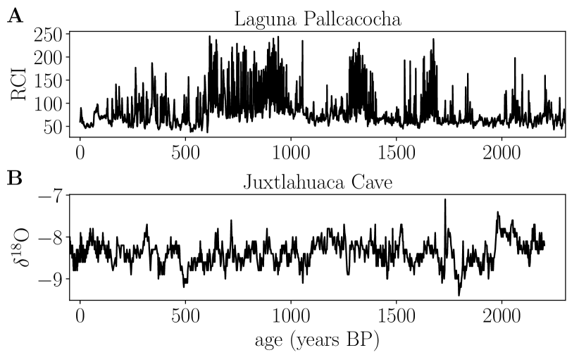
Figure 3: Paleoclimate data from (A) Laguna Pallcacocha Moy et al. (2002) (red color intensity) and (B) Juxtlahuaca cave Lachniet et al. (2012) (oxygen-18 residuals in units of ‰PDB). Data provided by https://www.ncdc.noaa.gov/.

The first data set (Fig. 3A) comprises the most recent $2300$ years ($N=4683$) of the red color intensity (RCI) data from Laguna Pallcacocha, a high-altitude lake sediment from southern Ecuador. The red color intensity serves as a proxy for rainfall intensity and has been related to the strength of historical El Niño Southern Oscillation (ENSO) events Moy et al. (2002). The data have a high temporal resolution with an average sampling time of $\left\langle\Delta t\right\rangle=0.49$ years with standard deviation $\sigma=0.27$ years. The values of the red color intensity vary between $37$ and $245$ with mean $\mu_{\text{RCI}}=96.7$ and standard deviation $\sigma_{\text{RCI}}=42.9$. High values of the RCI correspond to light colored laminae in the sediment and are associated with strong rainfall events triggered by moderate to strong warm ENSO episodes (El Niño events) Moy et al. (2002).

The second data set (Fig. 3B) consists of oxygen isotope ratios ($\delta^{18}$O) of the past $2250$ years ($N=1218$) recorded in a stalagmite from Juxtlahuaca cave in the Basin of Mexico Lachniet et al. (2012). This data set has also been related to rainfall variability in that region mostly affected by the strength of the North American summer monsoon. The latter is known to be affected by ENSO, where warm ENSO episodes lead to a weakened summer monsoon in this area and vice versa. This second data set has a larger average sampling time of $\left\langle\Delta t\right\rangle=1.8$ years with standard deviation $\sigma=0.86$ years. The proxy values vary between $-9.4$ ‰PDB (Peedee Belemnite) and $-7.1$ ‰PDB with mean $\mu_{\delta^{18}\text{O}}=-8.4$ ‰PDB and standard deviation $\sigma_{\delta^{18}\text{O}}=0.29$ ‰PDB. More negative values indicate higher rainfall amounts and less negative values less rainfall in the study area Lachniet et al. (2012).

IV.2 Analysis procedure

We analyze both data sets using windowed recurrence network analysis. That is, after reconstructing the phase space of the system, we take the first $W$ points of the time series, construct a recurrence network as described in Sec. II.3 and calculate the transitivity of the network. We focus here on transitivity as the only network measure, since the results shown in Sec. III for the two model systems indicate that the obtained results could be slightly more robust than for the average path length. Then we move the window and repeat the analysis, such that we end up with a time series of network measures. We assign the most recent time of the $W$ data points to the network measure as it is the result of the system dynamics up to this point. In order to characterize at which points in time the system exhibits extraordinary behavior, we use surrogate data to estimate significance levels Schreiber and Schmitz (2000). Our surrogates are created by randomly drawing $W$ embedded state vectors from the time series and calculating the transitivity of the corresponding recurrence network. This is repeated $N_{\text{surr}}=500$ times and two-sided $95\%$ significance levels are estimated using the $2.5$th and the $97.5$th percentile of the resulting network measures for the surrogates. This kind of analysis has already been shown to deliver valuable insights into the variability of the climate of the past Donges et al. (2011a, b, 2015a). It should be noted that the analysis of recurrence networks itself does not require regular sampling but can handle non-uniformly sampled data. Still, the reconstruction of the phase space is required prior to this analysis. As we have seen in the previous section that the results from interpolated time series perform quite well and because the interpretation of the results is not very clear for non-uniformly sampled data, we here use interpolated data.

We perform the windowed recurrence network analysis for different window widths, embedding dimensions and different methods to reconstruct the phase space. For each of the methods, we vary the internal embedding parameter, i. e. the delay time $\tau$ for time delay embedding and the number of neighboring points included when estimating the derivatives using discrete Legendre polynomials and MoTaBaR to check the robustness of the results. We chose to use linear interpolation for time delay embedding to get the required regular sampling of the data and compare the results to those obtained with differential embedding. According to the results obtained for the phase space reconstruction for the model systems (Sec. III), we use spline interpolation and scale the data to unit variance before constructing the recurrence networks for discrete Legendre polynomials. For MoTaBaR, we use the internal interpolation routine and also scale the data to unit variance. We vary the embedding dimension between $3$ and $6$ and choose window lengths of $W=\left[100,150,200,250,500\right]$. For time delay embedding, we vary the delays between $0$ and $50$ for Laguna Pallcacocha and between $0$ and $100$ for Juxtlahuaca cave. For differential embedding, we consider values of $p$ between $2$ and $20$ and for MoTaBaR, we vary $N_{mtb}$ between $10$ and $50$.

IV.3 Results

Figure 4 shows the results for the two data sets and three methods mentioned above for embedding dimension $m=4$.

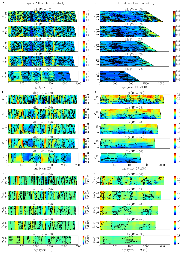
Figure 4: Network transitivity $\mathcal{T}$ as a function of age of Laguna Pallcacocha (left panels) and Juxtlahuaca cave (right panels) data sets for embedding dimension $m=4$, different phase space reconstructions and different window widths $W$. (A,B) Time delay embedding for varying delay times $\tau$. (C,D) Differential embedding with discrete Legendre polynomials and different values of the number of neighboring points $p$. (E,F) Differential embedding using MoTaBaR when varying the number of included points $N_{mtb}$.

This dimension has been chosen in accordance with the false nearest neighbor criterion Kennel, Brown, and Abarbanel (1992). In fact, when further increasing the embedding dimension, we do not observe significant changes in the results.

For Laguna Pallcacocha and time delay embedding (Fig. 4A), we identify four to five periods in which the network transitivity is significantly above that of the surrogate data. Also, we identify one to two periods with significantly lower transitivity. We observe that the timing of those anomalies shifts to more recent times when increasing the window width. This can be understood when recalling that we assign the most recent time to our time windows. For differential embedding using discrete Legendre polynomials to estimate the derivatives (Fig. 4C), we find similar but not identical significant periods. In general, the significant periods are wider, in particular for higher values of $W$ such that there is no clear separation between some periods like for time delay embedding. Also, the percentage of windows with significant values of the transitivity is higher than for time delay embedding. For differential embedding using MoTaBaR (Fig. 4E), we observe a rather stable behavior when varying the number of utilized points, but we also observe more and shorter significant regimes with different timings than those identified by the other two methods. Additionally, the minimum/maximum values of the network transitivity are larger/smaller than those obtained with time delay embedding and differential embedding using discrete Legendre polynomials.

The aforementioned behavior and the different timing of the identified significant periods is highlighted in more detail in Fig. 5.

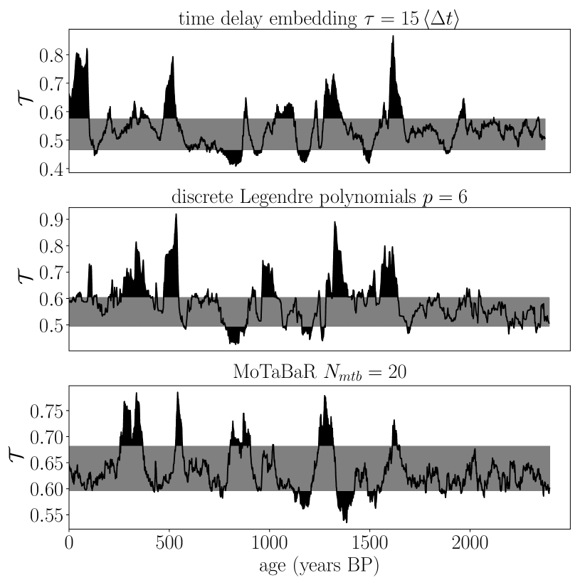
Figure 5: Network transitivity $\mathcal{T}$ as a function of age for the Laguna Pallcacocha data set using embedding dimension $m=4$, window width $W=200$ and different phase space reconstruction methods. For time delay embedding, the delay time is $\tau=15\left\langle\Delta t\right\rangle$; for differential embedding with discrete Legendre polynomials, the number of neighboring points is $p=6$; and for differential embedding using MoTaBaR, the number of included points is $N_{mtb}=20$.

Here, we choose the delay time to be $\tau=15\left\langle\Delta t\right\rangle$. This choice is in accordance with the first zero of the autocorrelation function of the time series using an estimator that can handle non-uniformly sampled data Rehfeld et al. (2011). For the discrete Legendre polynomials, we choose $p=6$. The estimator from Gibson suggests $p=2$, but in order to also estimate the higher order derivatives, we prefer to choose a slightly larger number of neighbors as already discussed in Sec. III. For MoTaBaR, the results do not vary a lot depending on the number of included points, so we decided to have a closer look at $N_{mtb}=20$. We see that the results for time delay embedding and discrete Legendre polynomials generally are in good agreement though some periods are more pronounced in either of the methods. For MoTaBaR, we partially find significant deviations from the surrogates at the same time as for the other methods, but we also observe shifts in timing and even opposite behavior as for example around $900$ years before present (BP). This highlights that it is not enough to consider a single analysis method or a single analysis parameter to infer information about the variability of the past climate. Instead, to gain confidence in the analysis results, several methods and a broad range of analysis parameters should be considered and checked for robustness.

The Laguna Pallcacocha RCI data set has previously been related to the succession of moderate to strong El Niño events. Moy et al. Moy et al. (2002) found that the frequency of those events has increased after $7000$ years BP and declined again from about $1200$ years BP onward. Here we do not analyze the number of individual El Niño events but rather aim at detecting general nonlinear changes and dynamical regime shifts in the climate signal represented by the considered proxy. Periods such as the Little Ice Age (LIA) or the Medieval Climate Anomaly (MCA) have been well expressed in North Atlantic climate proxies and Northern Hemisphere temperature trends have been argued to also influence ENSO and the position of the Intertropical Convergence zone (ITCZ) and, thus, Southern Hemisphere climate Novello et al. (2016). Starting from the past, we find consistent anomalies in recurrence network transitivity estimated using time delay embedding and discrete Legendre polynomials in the periods from (i) $2000-1950$ years BP, (ii) $1650-1550$ years BP, (iii) $1380-1275$ years BP, (iv) $870-750$ years BP, (v) $540-470$ years BP, (vi) $400-300$ years BP, and (vii) $100-0$ years BP. Generally, the anomalies start and finish slightly earlier for differential embedding using discrete Legendre polynomials than for time delay embedding. The first anomalies (i) and (ii) are similarly pronounced for both methods and might be related to the Roman Warm Period in Europe. This episode of rather stable warm temperatures might also have affected Southern Hemisphere climate by influencing SST temperatures in the Pacific leading to changes in ENSO. The latter is also visible in the MoTaBaR results. Anomaly (iii) is rather pronounced and might relate to changes in ENSO frequency around $1200$ years BP as observed by Moy et al Moy et al. (2002). Anomaly (iv) shows a significantly reduced network transitivity and co-occurred with the termination of the MCA. Vuille et al. determined this episode to be around $1050-850$ years BP in the Southern Hemisphere Vuille et al. (2012). The MCA in South America is associated with dryer climate due to a weakened South American monsoon system responding to anomalously high Northern Hemisphere temperatures. During this interval, we cannot observe consistent significant signals in the network transitivity across the different methods. Still, the anomaly we observe between $870-750$ years BP is likely the result of a change towards more complex climate variability as compared to the relatively stable climate during the MCA. Anomalies (v) and (vi) show significantly enhanced network transitivity and can be associated with the LIA that has been found to be around $350-130$ years BP in that area Vuille et al. (2012). Finally, anomaly (vii) can be related to the onset of the Current Warm Period and the associated recent climate change. Also, it should be mentioned that we find two periods where we observe inconsistencies between time delay embedding and differential embedding using discrete Legendre polynomials, one around $1500$ years BP and the other one around $1000$ years BP. For those periods, we cannot draw any conclusions about whether something significant happened, even though for the second time interval, we might expect to find signatures of the onset of the MCA.

Unlike for the Laguna Pallcacocha record, for the Juxtlahuaca cave, we generally cannot identify consistent periods during which the network transitivity shows significant anomalies over the full considered parameter range. For time delay embedding (Fig. 4B), we observe some elevated values in the very past and during more recent times together with some significantly reduced values around $500$ to $700$ years BP, but the timing varies a lot with both, the delay time $\tau$ and window width $W$. For differential embedding using discrete Legendre polynomials (Fig. 4D), we find that for higher values of $p$, almost all values of the transitivity are significantly above those of the surrogate data. This may be understood when recalling that higher values of $p$ increasingly smoothen the data corresponding to a low-pass filter. At some value of $p$ that also depends on the sampling rate, the time series becomes too flat, which is probably what happens here. For lower values of $p$ we observe a similar pattern as for time delay embedding, which is for some window widths also more localized. For differential embedding using MoTaBaR (Fig. 4F), we also find some significantly reduced values of the transitivity at similar times as for the other methods. Although these seem to be more robust than the other results, they appear still much less reliable than the results obtained for the Laguna Pallcacocha data set. Also, we observe again, that the values of the transitivity obtained with MoTaBaR are generally higher than those obtained with the other methods but in this case show some very high but no very low values.

The Juxtlahuaca cave record has been previously used to reconstruct rainfall over the past $2500$ years in the Basin of Mexico and related drought conditions to cultural change in this area. It has been argued that not only changes in mean conditions but also changes in climate variability can foster cultural change Donges et al. (2011b, 2015a). However, from the perspective of recurrence analyses, we cannot make any reliable statements for this data set. In turn, other more suitable records need to be obtained and analyzed to further examine the aforementioned relation.

V Conclusions

The reconstruction of a system’s phase space from measured data is an important step in the nonlinear analysis of real-world time series in many fields of application. However, care has to be taken in choosing an appropriate embedding, in particular when the data are non-uniformly sampled and noisy. For two paradigmatic model systems, we have used recurrence network measures to systematically compare the reference attractor to system attractors reconstructed using time delay embedding and differential embedding for different methods to estimate derivatives. When varying the noise level of the data and the shape of the distribution of the non-uniform sampling intervals, we found that differential embedding using discrete Legendre polynomials or Moving Taylor Bayesian Regression can be an alternative to time delay embedding for reconstructing the phase space of a system.

We also studied two precipitation sensitive paleoclimate proxy records from Ecuador and Mexico by combining windowed recurrence network analysis and different methods for phase space reconstruction. We found that the Laguna Pallcacocha data set from southern Ecuador gives robust results when varying embedding and network analysis parameters and therefore seems to be well-suited for such an analysis. Anomalies detected are in general in good agreement for two of the three considered methods but partially differ significantly for the third, highlighting that different phase space reconstructions should be compared before interpreting the results. We could relate the detected anomalies to known episodes of past climate change such as the Medieval Climate Anomaly and the Little Ice Age. Our corresponding results are consistent with previous work demonstrating that those periods, even though most pronounced in the Northern Hemisphere, have also left significant imprints in past climate variability of the Southern Hemisphere. For the Juxtlahuaca cave data set from southern Mexico, we could not identify robust anomalies using any of the methods applied. Thus, we have to conclude that this data set does not seem to be suitable to make any well-grounded statements about the variability of rainfall and possible regime shifts when using windowed recurrence network analysis. In turn, this shows that not all paleoclimate data sets are suited for this kind of analysis, and care has to be taken when analyzing paleoclimate time series with recurrence networks and related techniques. It is necessary to test the results for robustness by varying the different analysis parameters and comparing the results to draw reliable conclusions.

When respecting these insights for analyzing non-uniformly and noisy data in the paleoclimatologic context, we find that a framework of different phase space reconstruction methods combined with windowed recurrence network analysis and the associated robustness tests can be used to gain valuable insights into past climate variability. Thus, it should be further used to better understand and systematically study the climate of the past as this might help to better anticipate possible future changes.

*

Appendix A Estimating derivatives using discrete Legendre polynomials

In order to derive the formula for estimating the derivatives of a time series using discrete Legendre polynomials (Eq. (6)), we assume a discrete set of one-dimensional data $\left\{x_{i}\right\}_{i=1}^{N}$ with irregular sampling intervals $\Delta t_{i,n}=t_{i+n}-t_{i}$. We can apply a discrete linear filter

$$\omega_{j}(t_{i}) =\sum_{n=-p}^{p}r_{j,p,n}^{(i)}x(t_{i}+\Delta t_{i,n})$$ (16)

to the data and perform a Taylor expansion for small $\Delta t_{i,n}$ yielding

$$\omega_{j}(t_{i}) =\sum_{n=-p}^{p}r_{j,p,n}^{(i)}\left[\sum_{\nu=0}^{\infty}\dfrac{(\Delta t_{i,n})^{\nu}}{\nu!}\dfrac{d^{\nu}}{dt^{\nu}}x_{i}\right]$$

$$=\sum_{\nu=0}^{\infty}\dfrac{1}{\nu!}\dfrac{d^{\nu}}{dt^{\nu}}x_{i}\sum_{n=-p}^{p}(\Delta t_{i,n})^{\nu}r_{j,p,n}^{(i)}.$$ (17)

As we aim at deriving an expression for $\omega_{j}(t_{i})$ that is proportional to the $j$th derivative, we have to choose the filter function $r_{j,p,n}^{(i)}$ such that it is orthogonal to $(\Delta t_{i,n})^{\nu}$ for $\nu<j$:

$$\sum_{n=-p}^{p}(\Delta t_{i,n})^{\nu}r_{j,p,n}^{(i)} =0.$$ (18)

It can be shown that the discrete Legendre polynomials defined by the recursion (7) are mutually orthonormal filters, that is, they satisfy

$$\sum_{n=-p}^{p}r_{k,p,n}^{(i)}r_{l,p,n}^{(i)} =\delta_{k,l}$$

with $\delta_{k,l}$ being the Kronecker Delta. Thus, condition (18) holds and the Taylor expansion (17) reduces to

$$\omega_{j}(t_{i}) =\dfrac{1}{j!}\dfrac{d^{j}}{dt^{j}}x_{i}\sum_{n=-p}^{p}(\Delta t_{i,n})^{j}r_{j,p,n}^{(i)}$$

to leading order. Equating this result with Eq. (16) yields the desired result (6)

$$\dfrac{d^{j}}{dt^{j}}x_{i} \approx\dfrac{j!}{c_{j,p}(\Delta t_{i,n})}\sum_{n=-p}^{p}r_{j,p,n}^{(i)}x_{i+n},$$

relating the $j$th derivative of $x_{i}$ to the data points $\left\{x_{i+\mu}\right\}_{\mu=-p}^{p}$ of the time series. For given $p$, the discrete Legendre polynomials $r_{j,p,n}^{(i)}$ can easily be calculated numerically using the recursive relation (7) and the normalization condition (8).

References

- Marwan et al. (2007) N. Marwan, M. C. Romano, M. Thiel, and J. Kurths, “Recurrence plots for the analysis of complex systems,” Physics Reports 438, 237–329 (2007).
- Donges et al. (2011a) J. F. Donges, R. V. Donner, K. Rehfeld, N. Marwan, M. H. Trauth, and J. Kurths, “Identification of dynamical transitions in marine palaeoclimate records by recurrence network analysis,” Nonlinear Processes in Geophysics 18, 545–562 (2011a).
- Rehfeld et al. (2011) K. Rehfeld, N. Marwan, J. Heitzig, and J. Kurths, “Comparison of correlation analysis techniques for irregularly sampled time series,” Nonlinear Processes in Geophysics 18, 389–404 (2011).
- Donges et al. (2015a) J. F. Donges, R. V. Donner, N. Marwan, S. F. M. Breitenbach, K. Rehfeld, and J. Kurths, “Non-linear regime shifts in Holocene Asian monsoon variability: potential impacts on cultural change and migratory patterns,” Climate of the Past 11, 709–741 (2015a).
- Schleussner et al. (2016) C.-F. Schleussner, J. F. Donges, R. V. Donner, and H. J. Schellnhuber, “Armed-conflict risks enhanced by climate-related disasters in ethnically fractionalized countries,” Proceedings of the National Academy of Sciences 113, 9216–9221 (2016).
- Kennett et al. (2012) D. J. Kennett, S. F. M. Breitenbach, V. V. Aquino, Y. Asmerom, J. Awe, J. U. L. Baldini, P. Bartlein, B. J. Culleton, C. Ebert, and C. Jazwa et al., “Development and disintegration of Maya political systems in response to climate change,” Science 338, 788–791 (2012).
- Carleton, Campbell, and Collard (2017) W. C. Carleton, D. Campbell, and M. Collard, “Increasing temperature exacerbated classic maya conflict over the long term,” Quaternary Science Reviews 163, 209 – 218 (2017).
- Whitney (1936) H. Whitney, “Differentiable manifolds,” Annals of Mathematics 37, 645–680 (1936).
- Takens (1980) F. Takens, “Detecting strange attractors in turbulence,” in Lecture Notes in Mathematics (Springer Science and Business Media, 1980) pp. 366–381.
- Mañé (1981) R. Mañé, “On the dimension of the compact invariant sets of certain non-linear maps,” Lecture Notes in Mathematics, Berlin Springer Verlag 898, 230 (1981).
- Packard et al. (1980) N. H. Packard, J. P. Crutchfield, J. D. Farmer, and R. S. Shaw, “Geometry from a time series,” Physical Review Letters 45, 712–716 (1980).
- Casdagli et al. (1991) M. Casdagli, S. Eubank, J. Farmer, and J. Gibson, “State space reconstruction in the presence of noise,” Physica D 51, 52 – 98 (1991).
- Kantz and Schreiber (2004) H. Kantz and T. Schreiber, Nonlinear time series analysis, 2nd ed. (Cambridge University Press, 2004).
- Abarbanel et al. (1993) H. D. I. Abarbanel, R. Brown, J. J. Sidorowich, and L. S. Tsimring, “The analysis of observed chaotic data in physical systems,” Reviews of Modern Physics 65, 1331–1392 (1993).
- Fraser and Swinney (1986) A. M. Fraser and H. L. Swinney, “Independent coordinates for strange attractors from mutual information,” Physical Review A 33, 1134–1140 (1986).
- Gibson et al. (1992) J. F. Gibson, J. D. Farmer, M. Casdagli, and S. Eubank, “An analytic approach to practical phase space reconstruction,” Physica 57D (1992).
- Kennel, Brown, and Abarbanel (1992) M. B. Kennel, R. Brown, and H. D. I. Abarbanel, “Determining embedding dimension for phase-space reconstruction using a geometrical construction,” Physical Review A 45, 3403–3411 (1992).
- Hirata and Aihara (2017) Y. Hirata and K. Aihara, “Dimensionless embedding for nonlinear time series analysis,” Phys. Rev. E 96, 032219 (2017).
- Ozken et al. (2015) I. Ozken, D. Eroglu, T. Stemler, N. Marwan, G. B. Bagci, and J. Kurths, “Transformation-cost time-series method for analyzing irregularly sampled data,” Physical Review E 91, 062911 (2015).
- Rehfeld and Kurths (2014) K. Rehfeld and J. Kurths, “Similarity estimators for irregular and age-uncertain time series,” Climate of the Past 10, 107–122 (2014).
- Heitzig (2013) J. Heitzig, “Moving Taylor Bayesian Regression for nonparametric multidimensional function estimation with possibly correlated errors,” SIAM Journal on Scientific Computing 35, A1928–A1950 (2013).
- Donner et al. (2010a) R. V. Donner, Y. Zou, J. F. Donges, N. Marwan, and J. Kurths, “Recurrence networks — a novel paradigm for nonlinear time series analysis,” New Journal of Physics 12, 033025 (2010a).
- Donner et al. (2011a) R. V. Donner, M. Small, J. F. Donges, N. Marwan, Y. Zou, R. Xiang, and J. Kurths, “Recurrence-based time series analysis by means of complex network methods,” International Journal of Bifurcation and Chaos 21, 1019–1046 (2011a).
- Donner et al. (2010b) R. V. Donner, Y. Zou, J. F. Donges, N. Marwan, and J. Kurths, “Ambiguities in recurrence-based complex network representations of time series,” Physical Review E 81, 015101 (2010b).
- Donner et al. (2011b) R. V. Donner, J. Heitzig, J. F. Donges, Y. Zou, N. Marwan, and J. Kurths, “The geometry of chaotic dynamics — a complex network perspective,” The European Physical Journal B 84, 653–672 (2011b).
- Lorenz (1963) E. N. Lorenz, “Deterministic nonperiodic flow,” Journal of the Atmospheric Sciences 20, 130–141 (1963).
- Rössler (1976) O. Rössler, “An equation for continuous chaos,” Physics Letters A 57, 397 – 398 (1976).
- Xiang et al. (2012) R. Xiang, J. Zhang, X.-K. Xu, and M. Small, “Multiscale characterization of recurrence-based phase space networks constructed from time series,” Chaos 22, 013107 (2012).
- Jacob et al. (2016) R. Jacob, K. Harikrishnan, R. Misra, and G. Ambika, “Characterization of chaotic attractors under noise: A recurrence network perspective,” Communications in Nonlinear Science and Numerical Simulation 41, 32 – 47 (2016).
- Moy et al. (2002) C. M. Moy, G. O. Seltzer, D. T. Rodbell, and D. M. Anderson, “Variability of el niño southern oscillation activity at millennial timescales during the holocene epoch,” Nature 420, 162 (2002).
- Lachniet et al. (2012) M. S. Lachniet, J. P. Bernal, Y. Asmerom, V. Polyak, and D. Piperno, “A 2400 yr Mesoamerican rainfall reconstruction links climate and cultural change,” Geology 40, 259–262 (2012).
- Schreiber and Schmitz (2000) T. Schreiber and A. Schmitz, “Surrogate time series,” Physica D: Nonlinear Phenomena 142, 346 – 382 (2000).
- Donges et al. (2011b) J. F. Donges, R. V. Donner, M. H. Trauth, N. Marwan, H.-J. Schellnhuber, and J. Kurths, “Nonlinear detection of paleoclimate-variability transitions possibly related to human evolution,” Proceedings of the National Academy of Sciences 108, 20422–20427 (2011b).
- Novello et al. (2016) V. F. Novello, M. Vuille, F. W. Cruz, N. M. Stríis, M. S. de Paula, R. L. Edwards, H. Cheng, I. Karmann, P. F. Jaqueto, and R. I. F. Trindade et al., “Centennial-scale solar forcing of the South American monsoon system recorded in stalagmites,” Scientific Reports 6, 24762 (2016).
- Vuille et al. (2012) M. Vuille, S. J. Burns, B. L. Taylor, F. W. Cruz, B. W. Bird, M. B. Abbott, L. C. Kanner, H. Cheng, and V. F. Novello, “A review of the South American monsoon history as recorded in stable isotopic proxies over the past two millennia,” Climate of the Past 8, 1309–1321 (2012).
- Donges et al. (2015b) J. F. Donges, J. Heitzig, B. Beronov, M. Wiedermann, J. Runge, Q. Y. Feng, L. Tupikina, V. Stolbova, R. V. Donner, and N. Marwan et al., “Unified functional network and nonlinear time series analysis for complex systems science: The pyunicorn package,” Chaos 25, 113101 (2015b).