IFT-UAM/CSIC-18-005
FTUAM-18-2
January 2018
Non-Perturbative Renormalisation and Running
of BSM Four-Quark Operators in QCD
![]()
P. Dimopoulosa,b, G. Herdoízac,d, M. Papinuttoe, C. Penac,d, D. Pretic,f, and A. Vladikasg
a Centro Fermi - Museo Storico della Fisica e Centro Studi e Ricerche “Enrico Fermi”,
Compendio del Viminale, Piazza del Viminale 1, 00184 Rome, Italy
b Dipartimento di Fisica, Università di Roma Tor Vergata,
Via della Ricerca Scientifica 1, I-00133 Rome, Italy
c Instituto de Física Teórica UAM/CSIC,
c/Nicolás Cabrera 13-15, Universidad Autónoma de Madrid,
Cantoblanco E-28049 Madrid, Spain
d Departamento de Física Teórica, Universidad Autónoma de Madrid,
Cantoblanco E-28049 Madrid, Spain
e Dipartimento di Fisica, “Sapienza” Università di Roma, and INFN, Sezione di Roma
Piazzale A. Moro 2, I-00185 Roma, Italy
f INFN Sezione di Torino,
Via Pietro Giuria 1, I-10125 Turin, Italy
g INFN-Sezione di Tor Vergata, c/o Dipartimento di Fisica,
Università di Roma Tor Vergata, Via della Ricerca Scientifica 1,
I-00133 Rome, Italy
Abstract: We perform a non-perturbative study of the scale-dependent renormalisation factors of a complete set of dimension-six four-fermion operators. The renormalisation-group (RG) running is determined in the continuum limit for a specific Schrödinger Functional (SF) renormalisation scheme in the framework of lattice QCD with two dynamical flavours (). The theory is regularised on a lattice with a plaquette Wilson action and -improved Wilson fermions. For one of these operators, the computation had been performed in ref. [1]; the present work completes the study for the rest of the operator basis, on the same simulations (configuration ensembles). The related weak matrix elements arise in several operator product expansions; in transitions they contain the QCD long-distance effects, including contributions from beyond-Standard Model (BSM) processes. Some of these operators mix under renormalisation and their RG-running is governed by anomalous dimension matrices. In ref. [2] the RG formalism for the operator basis has been worked out in full generality and the anomalous dimension matrix has been calculated in NLO perturbation theory. Here the discussion is extended to the matrix step-scaling functions (matrix-SSFs), which are used in finite-size recursive techniques. We rely on these matrix-SSFs to obtain non-perturbative estimates of the operator anomalous dimensions for scales ranging from to .
1 Introduction
In lattice QCD, the renormalisation of composite operators is an important step towards obtaining estimates of hadronic low-energy quantities in the continuum limit. Quark masses, decay constants, form factors, etc. are extracted from matrix elements of such operators; see ref. [3] for a recent review of lattice flavour phenomenology. Of interest to the present work is the class of dimension-six, four-fermion composite fields, arising in operator product expansions (OPE), in which the heavier quark degrees of freedom are integrated out. For and many transitions ( stands for flavour here), the resulting weak matrix elements of these operators govern long-distance QCD effects. They can be reliably evaluated by applying an intrinsically non-perturbative approach. Lattice QCD is our regularisation of choice which, by combining theoretical and computational methods, allows for an evaluation of these quantities with errors that can be reliably estimated and systematically improved.
Here we address the problem of calculating the renormalisation parameters and their renormalisation group (RG)-running for the operators defined in Eq. (2.6) below. We opt for the lattice regularisation consisting in the Wilson plaquette gauge action and the -improved Wilson quark action. We renormalise the bare operators in the Schrödinger Functional (SF) renormalisation scheme. This problem has first been studied with Wilson fermions for the relatively simple case of the multiplicatively renormalisable operators of Eq. (2.6), both perturbatively [4] and non-perturbatively in the quenched approximation [5]. Subsequently results for have also been obtained with dynamical sea quarks [1]. (An analogous study with quenched Neuberger fermions may be found in ref. [6].) Recently the perturbative calculations have been extended in ref. [2] for the rest of the operator basis of Eq. (2.6). The present is a companion paper of this work, complementing it by providing non-perturbative results for the operators , computed in lattice QCD.
As stressed in refs. [7, 2], these operators, treated here in full generality, become relevant for a number of interesting processes, once specific physical flavours are assigned to their fermion fields. For example, with and (cf. Eq. (2.7)), the weak matrix element comprises leading long-distance contributions in the effective Hamiltonian formalism for neutral -meson oscillations in the Standard Model (SM). Allowing for beyond-Standard-Model (BSM) interactions introduces similar matrix elements of the remaining operators . In some lattice regularisations, the corresponding bare matrix elements are expressed in terms of the operators , with some important simplifications in their renormalisation properties [7, 8, 9]. In refs. [2] other flavour assignments are listed, leading to four-fermion operators related to the low-energy effects of transitions (– and – mixing) and to the effective weak Hamiltonian with an active charm quark. In the present work we will concentrate on the renormalisation and RG-runing of .
It is important to keep in mind that the sets and are parity-even and parity-odd components of operators with chiral structures (such as “left-left” or “left-right”) which ensure their transformation under specific irreducible chiral representations. Chiral symmetry may be broken by the regularisation (e.g. lattice Wilson fermions) but it is recovered by the continuum theory. An important consequence is that our results, obtained for the continuum RG-evolution of the parity-odd bases , are also valid for the parity-even ones .
The paper is organised as follows:
In section 2 we list the operators we
are studying and their basic renormalisation pattern. We also
derive their RG-equations, and define the evolution matrices and the renormalisation-group
invariant operators, which are scale- and scheme-independent quantities.
This is an abbreviated version of section 2 of ref. [2]. The interesting
feature of the renormalisation pattern of operators is that
they mix in pairs111This is not to be confused with the operator mixing of
(the operator arising in transitions in the Standard Model), which
mixes with when Wilson lattice fermions are used, and chiral
symmetry is broken by the regularisation.. In the case of , mixing is not an artefact of the lattice
regularisation, as it also happens in schemes where all symmetries of the continuum target
theory (QCD) are preserved; cf. ref. [7]. An important consequence of this property is that
the RG-running of these operators is governed by anomalous-dimension and RG-evolution
matrices, rather than scalar functions. The RG-evolution matrices are well known in NLO perturbation
theory; cf. refs. [10, 11]. Here, following ref. [2],
we use them in closed form, suitable for non-perturbative evaluations.
In section 3 we outline our strategy. First we
define the SF renormalisation conditions for the operators ; again this is
an abridged version of subsection 3.3 of ref. [2]. Next, we define
in the SF scheme
the matrix step-scaling functions (SSFs) as the RG-evolution matrices for a change of renormalisation scale by a fixed arbitrary factor; this factor is 2 in the present work. These are our basic lattice quantities,
computed for a sequence of lattice spacings, at fixed renormalised gauge coupling. They have a well defined continuum limit, which is obtained by extrapolation, as explained in the same section. Repeating the calculation for a range of renormalisation scales (i.e. a range of renormalised couplings) and interpolating our data points,
we finally have the SSFs as continuous polynomials of the gauge coupling, from which we obtain the anomalous dimension matrices, with NLO perturbation theory taking over only at scales.
In section 4 we present our results. Besides the aforementioned SSFs, RG-evolution matrices and anomalous-dimension matrices, we also compute the renormalisation matrices for
values of the gauge coupling corresponding to low-energy scales. These renormalisation factors
are needed, in order to renormalise the corresponding bare matrix elements at these hadronic scales.
The computation of the latter requires independent simulations on large physical lattices (of about
3-5 fm), which is beyond the scope of this work.
Appendix A collects additional tests of the comparision
between perturbative and non-perturbative RG evolution, including the
specific renormalisation scale range, [2 GeV, 3 GeV], considered
in ref. [12]. Further details about one-loop cutoff
effects in the SSFs are presented in Appendix B.
2 Renormalisation of four-quark operators
This section is an abridged version of sect. 2 of ref. [2], which we repeat here for completeness.
2.1 Renormalisation and mixing of four-quark operators
We recapitulate the main renormalisation properties of the four-fermion operators under study. These results have been obtained in full generality in ref. [7]. The absence of subtractions is elegantly implemented by using a formalism in which the operators consist of quark fields with four distinct flavours. A complete set of Lorentz-invariant operators is
| (2.6) |
where
| (2.7) |
. The operator subscripts obviously correspond to the labelling , , , , , , with . Repeated Lorentz indices, such as and are summed over. In the above expression round parentheses indicate spin and colour traces and the subscripts of the fermion fields are flavour labels. Note that operators are parity-even, and are parity-odd.
In the following we will assume a mass-independent renormalisation scheme. Renormalised operators can be written as
| (2.8) |
(summations over are implied), where the renormalisation matrices are scale-dependent and reabsorb logarithmic divergences, while are (possible) matrices of finite subtraction coefficients that only depend on the bare coupling. Throughout this work we use boldface symbols for the column vectors of four-fermion operator and the matrices which act on these vectors (e.g. , etc.) while their elements are indicated with explicit indices (e.g. , etc.). We also introduce a simplification in our notation, by dropping the superscripts , wherever no ambiguity arises. This should not be a problem as the symmetric operator bases and (symmetric under flavour exchange ) never mix with the antisymmetric ones and , and thus equations are valid separately for each basis.
The renormalisation matrices have the generic structure
| (2.19) |
Analogous expressions hold for and D. If chiral symmetry is preserved by the regularisation, both and D vanish. In the case of Wilson fermions, with chiral symmetry explicitly broken, we have , whereas due to residual discrete flavour symmetries ; this is the main result of ref. [7]. Therefore the left-left operators , which mediate Standard Model-allowed transitions, renormalise multiplicatively, while operators , which appear as effective interactions in extensions of the Standard Model, mix in pairs: and .
In conclusion, with Wilson fermions the parity-odd basis renormalises in a pattern analogous to that of a chirally symmetric regularisation, while the parity-even one has a more complicated renormalisation pattern due to the non-vanishing of . We will henceforth concentrate on the non-perturbative renormalisation of the parity-odd basis with Wilson fermions.
2.2 Renormalisation group equations
The scale dependence of renormalised quantities is governed by renormalisation group evolution. Denoting as the running momentum scale and the renormalisation scale where mass-independent renormalisation conditions are imposed, we have the following Callan-Symanzik equations for the gauge coupling and quark masses respectively:
| (2.20) | ||||
| (2.21) |
where is a flavour label. The scheme mass-independence implies that the Callan-Symanzik function and the mass anomalous dimension depend only on the coupling. Asymptotic perturbative expansions read
| (2.22) | ||||
| (2.23) |
Let us now turn to Euclidean correlation functions of gauge-invariant composite operators, of the form222To simplify the notation, we have omitted the dependence of on the coupling, the masses and the UV cutoff (e.g. the lattice spacing).
| (2.24) |
with . For concreteness we have opted for correlation functions of the parity-odd operators , which are the subject of the present work. Nevertheless, the results of this section apply to any set of operators that mix under renormalisation. The operators may be any convenient, multiplicatively renormalisable source field. For example they could be currents or densities (e.g. and/or ), or Schrödinger functional sources at the time-boundaries. The latter will be explicitly discussed in Sect. 3. Renormalised correlation functions satisfy the system of Callan-Symanzik equations
| (2.25) |
or, expanding the total derivative,
| (2.26) |
where is a matrix of anomalous dimensions describing the mixing of (cf. Eq. (2.27) below), and is the anomalous dimension of (defined in a way analogous to Eq. (2.27)). A possible term arising from the running of the gauge parameter of the action is omitted here, for reasons explained in ref. [2]. A convenient shorthand notation for the anomalous dimension matrix of the operators is thus
| (2.27) |
The operator anomalous dimensions admit perturbative expansions of the form
| (2.28) |
In standard fashion we can then derive
| (2.29) |
This result implies that the block-diagonal form of the renormalisation matrices (and ) of Eq. (2.19) induces the same block-diagonal structure for the anomalous dimension matrix . Thus the sums in Eqs. (2.27) and (2.29) simplify: for operator and its anomalous dimension there is no summation; for operators summations run over indices 2 and 3 only, and similarly for the operator sub-basis .
2.3 Evolution matrices and renormalisation group invariants
In order to obtain a solution of Eq. (2.27) in closed form, it is convenient to introduce the renormalisation group evolution matrix that evolves renormalised operators between scales333Restricting the evolution operator to run towards the IR avoids unessential algebraic technicalities below. The running towards the UV can be trivially obtained by taking . and :
| (2.30) |
Substituting the above into Eq. (2.27) we obtain for the running of
| (2.31) |
with initial condition . Note that the r.h.s. is a matrix product. Following a standard procedure, the above expression can be converted into a Volterra-type integral equation and solved iteratively, viz.
| (2.32) |
where as usual the notation denotes a Taylor expansion of the exponent, in which each term is an ordered (here -ordered) product. Explicitly, for a generic matrix function , we have
| (2.33) |
In the specific case of interest, , with a matrix function and a real function. To leading order (LO) we have that and the independence of the matrix from the coupling simplifies eq. (2.33), so that the becomes a standard exponential. One can then easily integrate the exponent in eq. (2.32) and obtain the LO approximation of the evolution matrix:
| (2.34) |
When next-to-leading order corrections are included, the T-exponential becomes non-trivial. Further insight is gained upon realising that the associativity property of the evolution matrix implies that it can actually be factorised in full generality as
| (2.35) |
and the matrix can be expressed in terms of a matrix , defined through
| (2.36) |
The matrix can be interpreted as the piece of the evolution operator containing contributions beyond the leading perturbative order. Putting everything together, we see that
| (2.37) |
and thus we make contact with the literature (see e.g. [11, 10]).
Upon inserting Eq. (2.37) in Eq. (2.31) we obtain for the RG equation
| (2.38) |
Expanding perturbatively we can check [2] that is regular in the UV, and all the logarithmic divergences in the evolution operator are contained in ; in particular,
| (2.39) |
Rewriting Eq. (2.30) as
| (2.40) |
and observing that the l.h.s. (respectively r.h.s.) is obviously independent of (respectively ), we conclude that these are scale-independent expressions. Thus we can define the vector of RGI operators as
| (2.41) |
where in the last step we use Eq. (2.39).
3 Schrödinger Functional renormalisation setup
In this section we introduce the finite volume Schrödinger Functional (SF) renormalisation schemes and the RG evolution matrix between scales separated by a fixed factor (i.e. the matrix-step-scaling function).
3.1 Renormalisation conditions
We first define Schrödinger Functional renormalisation schemes for the operator basis of Eq. (2.6). This section is an abridged version of sec. 3.3 of ref. [2]. We use the standard SF setup as described in [13], where the reader is referred for full details including unexplained notation.
We work with lattices of spatial extent and time extent ; here we opt for . Source fields are made up of boundary quarks and antiquarks,
| (3.42) | ||||
| (3.43) |
where are flavour indices, unprimed (primed) fields live at the () boundary, and is a Dirac matrix. The boundary fields are constrained to satisfy the conditions
| (3.44) |
and similarly for primed fields. This implies that the Dirac matrices must anticommute with , otherwise the boundary operators and vanish; thus may be either or ().
Renormalisation conditions are imposed in the massless theory, in order to obtain a mass-independent scheme by construction. They are furthermore imposed on the parity-odd four-quark operators of Eq. (2.6), since working in the parity-even sector would entail dealing with the extra mixing due to explicit chiral symmetry breaking with Wilson fermions, cf. Eq. (2.19). In order to obtain non-vanishing SF correlation functions, we then need a product of source operators with overall negative parity; taking into account the above observation about boundary fields, and the need to saturate flavour indices, the minimal structure involves three boundary bilinear operators and the introduction of an extra, “spectator” flavour (labeled as number 5, keeping with the notation in Eq. (2.7)). We thus end up with correlation functions of the generic form
| (3.45) | ||||
| (3.46) |
where is one of the five source operators
| (3.47) | ||||
| (3.48) | ||||
| (3.49) | ||||
| (3.50) | ||||
| (3.51) |
with
| (3.52) |
and similarly for , which is defined with the boundary fields exchanged between time boundaries; e.g etc. The constant is a sign that ensures for all possible indices444This time reversal property, besides being a useful numerical cross check of our codes, allows taking the average of and so as to reduce statistical fluctuations. From now on denotes this average.; it is easy to check that .We also use the two-point functions of boundary sources
| (3.53) | ||||
| (3.54) |
Finally, we define the ratios
| (3.55) |
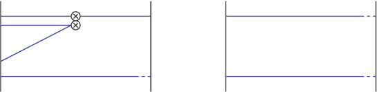
where is an arbitrary real parameter. The geometry of , and is illustrated in Fig. 1.
We can now impose Schrödinger functional renormalisation conditions on the ratio of correlation functions defined in Eq. (3.55), at fixed bare coupling , vanishing quark mass, and scale . For the renormalisable multiplicative operators we set
| (3.56) |
For operators that mix in doublets, we impose555S. Sint, private communication.
| (3.63) |
and similarly for . The product of boundary-to-boundary correlators in the denominator of Eq. (3.55) cancels the renormalisation of the boundary operators in , and therefore only contains anomalous dimensions of four-fermion operators. Following [14, 5, 1], conditions are imposed on renormalisation functions evaluated at , and the phase that parameterises spatial boundary conditions on fermion fields is fixed to . Together with the geometry of our finite box, this fixes the renormalisation scheme completely, up to the choice of boundary source, indicated by the index , and the parameter . The latter can in principle take any value, but we restrict our choice to .
One still has to check that the above renormalisation conditions are well-defined at tree-level. This is straightforward for Eq. (3.56), but not for Eq. (3.63): it is still possible that the matrix of ratios has zero determinant at tree-level, rendering the system of equations for the renormalisation matrix ill-conditioned. This is indeed obviously the case for , but the determinant vanishes also for other non-trivial choices of . In practice, out of the ten possible schemes one is only left with six, viz.666Note that schemes obtained by exchanging are trivially related to each other.
| (3.64) |
This property is independent of the choice of and . Thus, we are left with a total of 15 schemes for , and 18 for each of the pairs and .
Given the strong scheme dependence of the matrices (cf. Eq. (2.28)), a criterion has been devised in ref. [2] in order to single out the scheme with the smallest NLO anomalous dimension. This consists in choosing the scheme with the smallest determinant and trace of the matrix for each non-trivial anomalous dimension matrix. It turns out that the scheme defined by and satisfies these requirements in all cases (i.e. for the matrices related to and ). In the following we will present non-perturbative results for this scheme only777Although we have completed our analyses in all schemes discussed here, for reasons of economy of presentation we will not show these results. In any case, the and scheme displays the most reliable matching to perturbative RG-running at the electorweak scale..
3.2 Matrix-step-scaling functions and non-perturbative computation of RGI operators
In order to trace the RG evolution non-perturbatively, we introduce matrix-step-scaling functions (matrix-SSFs), defined as888The relative factor between the scales is arbitrary; one could introduce a that evolves from scale to scale . In this notation, our choice corresponds to .
| (3.65) |
The above definition generalises the step-scaling functions (SSFs) defined for quark masses [14] and multiplicatively renormalisable four-fermion operators [5] such as . Just like the anomalous dimension matrix , the matrix-SSF has a block-diagonal structure. So the above definition either refers to one of the two multiplicative operators , or to one of the four pairs of operators that mix under renormalisation; i.e. or . In the former cases is a real function, whereas in the latter cases it is a matrix of real functions. Again in what follows the superscripts will be suppressed.
The advantage of working with step-scaling functions is that they can be computed on the lattice with all systematic uncertainties under control. More concretely, we define the lattice matrix-SSF in a finite lattice; as repeatedly stated previously, in this work we set . Working in the chiral limit, at a given bare coupling (i.e. at a given finite UV cutoff ) , is defined as the following “ratio” of renormalisation matrices at two renormalisation scales and :
| (3.66) |
This quantity has a well defined continuum limit. For a sequence of lattice sizes , we tune the bare coupling (and thus the corresponding lattice spacing ) to a sequence of values which correspond to a constant renormalised squared coupling . Keeping fixed implies that the renormalisation scale is also held fixed. It is then straightforward to check that satisfies
| (3.67) |
Thus, the computation of the renormalisation matrices at a fixed value of the renormalised squared coupling and various values of the lattice sizes and , allows for a controlled extrapolation of the matrix-SSFs to the continuum limit.
The strategy for obtaining non-perturbative estimates of RGI operators proceeds in standard fashion: We start from a low-energy scale , implicitly defined by . The SSF for the coupling, defined as , is known for from ref. [15]. Thus we generate a sequence of squared couplings through the recursion , and compute recursively the matrix-SSFs which correspond to a sequence of physical lattice lengths (inverse renormalisation scales) . This is followed by the computation of
| (3.68) |
with . Here is thought of as a high-energy scale, safely into the perturbative regime, and as a low-energy scale, characteristic of hadronic physics. The RGI operators of Eq. (2.41) can finally be constructed as follows:
| (3.69) |
In other words, once we know the column of renormalised operators at a hadronic scale from a standard computation on a lattice of “infinite” physical volume (which is beyond the scope of the present paper), we can combine it with the non-perturbative evolution matrix (which is the result of this work) and the remaining -dependent factors at scale (known in NLO perturbation theory from ref. [2]), to obtain the RGI operators999The computation of operators (i.e. their physical matrix elements) must be known with a precision similar to that of the evolution matrix.. All factors on the r.h.s. must be known in the same renormalisation scheme, which here is the SF. The scheme dependence should cancel in the product of the r.h.s., since is scheme-independent. In practice a residual dependence remains due to the fact that is only known in perturbation theory (typically to NLO). Finally we stress that depends, through the operators , on the values of the quark masses; of course the result also depends on the flavour content of the QCD model under scrutiny (i.e. ).
We mentioned above that the matrix is known in NLO perturbation theory from ref. [2]. This statement requires a brief elucidation: is obtained by numerically integrating Eq. (2.38), using the NLO (2-loop) perturbative result for and the NNLO (3-loop) perturbative result for . In what follows this will be abbreviated as NLO-2/3PT. In line with ref. [2], also the present work devotes considerable effort to the investigation of the reliability of NLO-2/3PT at the scale .
3.3 Matrix-step-scaling functions and continuum extrapolations
We now turn to some practical considerations concerning the extrapolation of to the continuum limit , from which we obtain ; cf. Eq. (3.67). We stress that although fermionic and gauge actions are Symanzik-improved by the presence of bulk and boundary counter-terms, correlation functions with dimension-six operators in the bulk of the lattice, such as those defined in Eqs. (3.45) and (3.55), are subject to linear discretisation errors. Their removal could be achieved in principle by the subtraction of dimension-7 counter-terms, but their coefficients are not easy to determine in practice. We therefore expect linear cutoff effects and consequently fit with the Ansatz
| (3.70) |
In analogy to ref. [16], we explore the reliability of the above extrapolations with the help of the lowest-order perturbative expression for , which includes terms. In general the perturbative series for the operator renormalisation matrices has the form [16]
| (3.71) |
where in the limit the coefficients are -degree polynomials in up to corrections of . In particular the coefficient of the logarithmic divergence in is given by the one-loop anomalous dimension , and thus we parametrise as
| (3.72) |
with and . It is now easy to see that the one-loop perturbative expression for the matrix-SSF is given by
| (3.73) |
with
| (3.74) |
In the continuum limit ( with fixed) we have
| (3.75) |
The quantity
| (3.76) |
contains all lattice artefacts at . Results for are reported in Appendix B.
The “subtracted” matrix-SSF, defined as
| (3.77) |
also tends to in the continuum limit, but has the effects removed. We will also use this quantity when studying the reliability of the linear continuum extrapolations below.
3.4 Perturbative expansion of matrix-step-scaling functions
Once the continuum matrix-SSF has been computed for discrete values of the renormalised coupling , it is useful to interpolate the data so as to obtain as a continuous function. This is done by fitting the points by a suitably truncated polynomial
| (3.78) |
With only a few () points at our disposal, the fit stability is greatly facilitated by fixing the first two coefficients (matrices) and respectively to their LO and NLO perturbative values, leaving as the only free fit parameter. We will now derive the perturbative coefficients and .
Since the operator RG-running is coupled to that of the strong coupling, we also need the LO and NLO coefficients of its step-scaling function (SSF); i.e.
| (3.79) |
Given the strong coupling value at a renormalisation scale , its SSF is defined as ; cf. ref.[17]. Combining this definition with that of the Callan-Symanzik -function of Eq. (2.20), we find that
| (3.80) |
Plugging the NLO expansion of Eq. (2.22) in the above and taking Eq. (3.79) into account, we obtain the coefficients of the coupling SSF
| (3.81) | ||||
| (3.82) |
Matrix-SSFs for four-quark operators have been introduced in Eq. (3.65). In order to calculate the coefficients and of its perturbative expansion Eq. (3.78), we first write down the LO evolution matrix as
| (3.83) |
Furthermore, the matrix of Eq. (3.65) has the NLO perturbative expansion (cf. ref. [2] and references therein)
| (3.84) |
from which the inverse matrix is readily obtained:
| (3.85) |
We arrive at the last expression on the rhs by inserting the power-series expansion of form Eq. (3.79). Substituting the various terms in Eq. (3.65) by the perturbative series (LABEL:eq:U_LO), (3.84) and (3.85), we find
| (3.86) | ||||
| (3.87) |
From the first expression obtained for we see explicitly that corrections to do not contribute (i.e. terms with are absent), in accordance with the fact that the term of already contains all NLO contributions. The second expression for is obtained by using the property (cf. ref. [2] and references therein)
| (3.88) |
Remarkably, the final result for is the exact analogue of the one found for operators that renormalise multiplicatively, cf. e.g. Eq. (6.6) in [4].
4 Non-perturbative computations
Our simulations are performed using the lattice regularisation of QCD consisting of the standard plaquette Wilson action for the gauge fields and the non-perturbatively improved Wilson action for dynamical fermions. The fermion action is Clover-improved with the Sheikoleslami-Wohlert (SW) coefficient determined in [18]. The matrix-SSFs are computed at six different values of the SF renormalised coupling, corresponding to six physical lattice extensions (i.e six values of the renormalisation scale ). For each physical volume three different values of the lattice spacing are simulated, corresponding to lattices with ; this is achieved by tuning the bare coupling so that the renormalised coupling (and thus ) is approximately fixed. At the same we also generate configuration ensembles at twice the lattice volume; i.e. respectively. We compute and and thus ; cf. Eq. (3.66). The gauge configuration ensembles used in the present work and the tuning of the lattice parameters are taken over from ref. [19] where all technical details concerning these dynamical fermion simulations are discussed. As pointed out in [19], the gauge configurations at the three weakest couplings have been produced using the one-loop perturbative estimate of [20], except for and . For these two cases and for the three strongest couplings the two-loop value of [21] has been used.
Statistical errors are computed by blocking (binning) the measurements of each renormalisation parameter and calculating the bootstrap error on the binned averages. In order to take their autocorrelation length into account, we determine the block-size for which the bootstrap error of a given renormalisation parameter reaches a plateau. This varies for each of the four matrix elements of a given renormalisation matrix. We conservatively fix our preferred block-size to the maximum of all four cases, and estimate our statistical error accordingly. We crosscheck our results by also applying the Gamma method error analysis of ref. [22], and by varying the summation-window size. The results from the two methods agree within the (relevant) uncertainties.
Numerical results for and , computed from Eq. (3.63), are collected in Tabs. 7 and 8. The reason we prefer quoting the inverse of is that it is this quantity which is required for the computation of the matrix-SSFs; cf. Eq. (3.66).
4.1 Lattice computation of matrix-functions
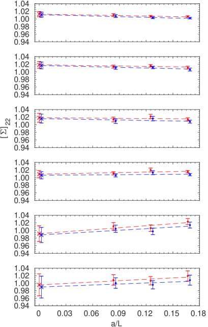
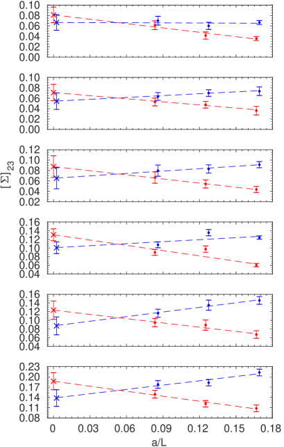
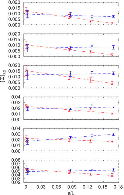
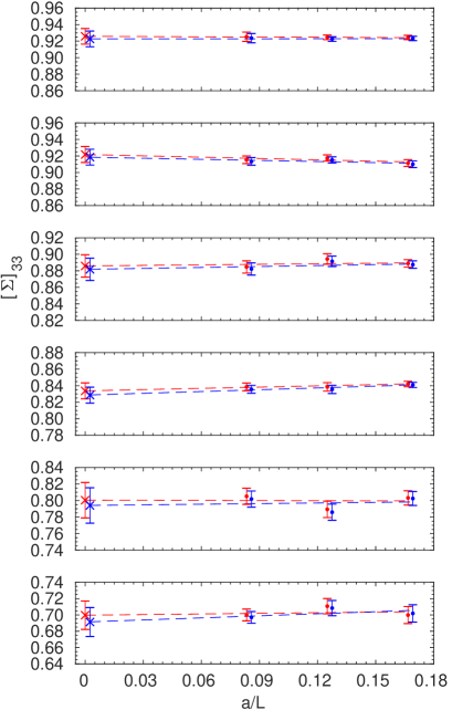
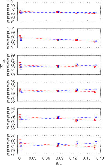
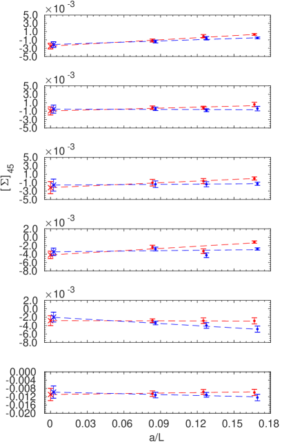
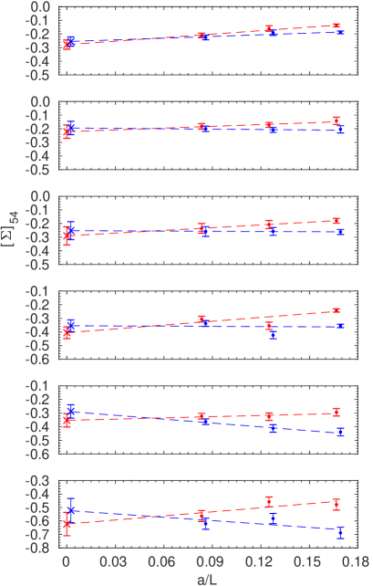
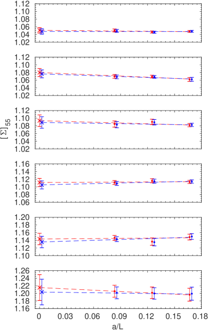
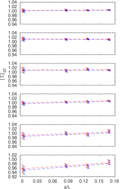
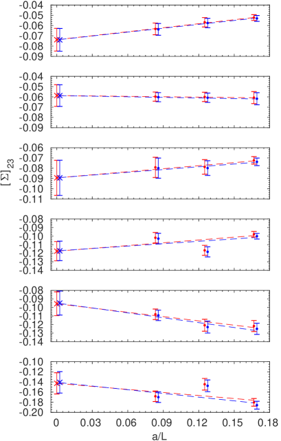
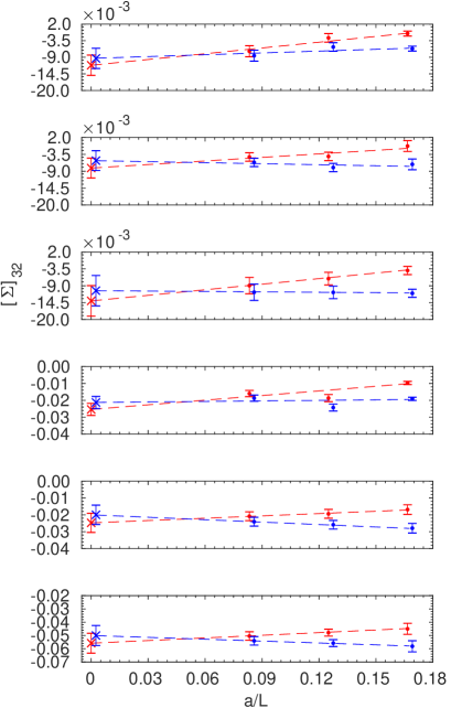
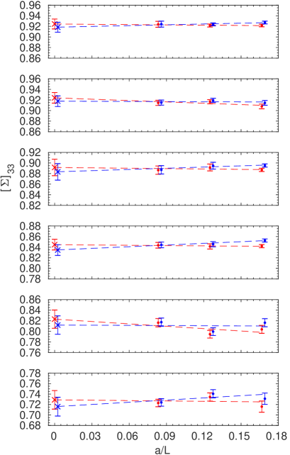
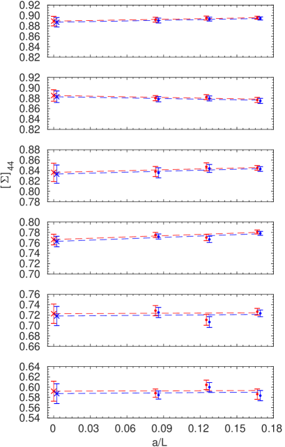
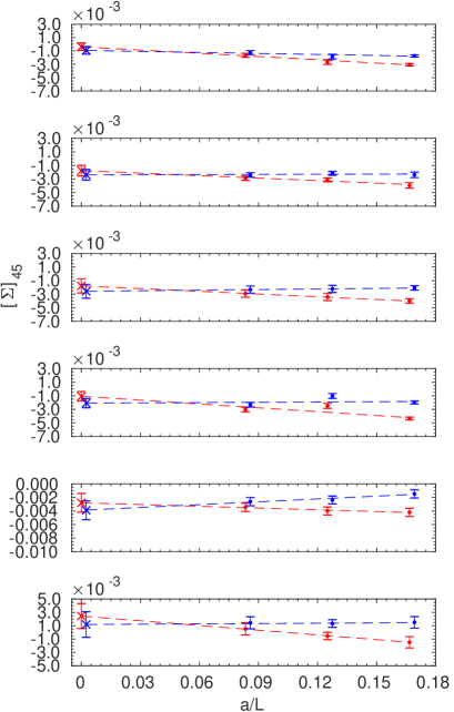
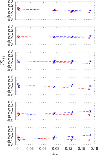
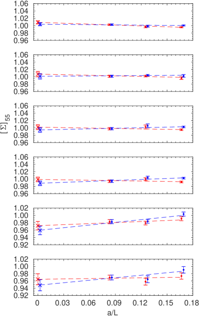
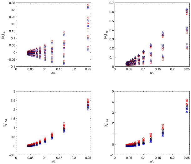
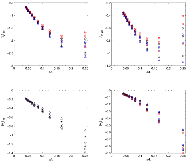
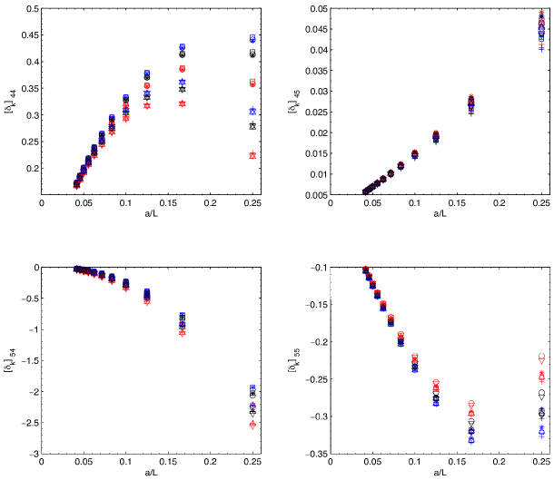
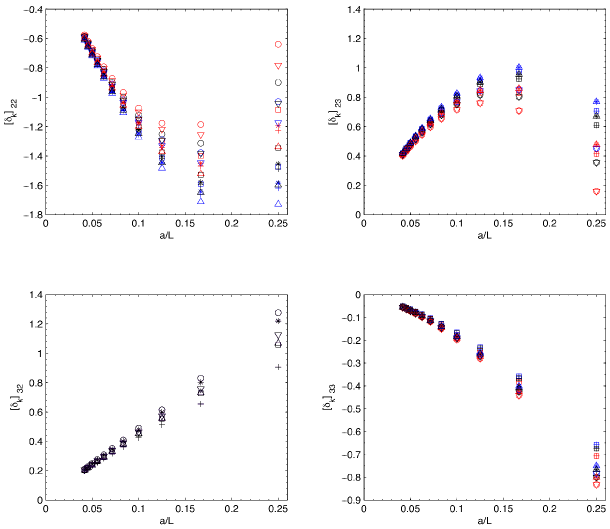
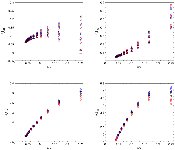
We perform linear extrapolations in of both and (cf. Eqs. (3.70) and (3.77)), so as to crosscheck the reliability of the continuum value . The extrapolation results can be found in Tabs. 1 and 2, as well as in Figs. 6,7,8, and 9. In most cases both extrapolations agree; at worst the agreement is within two standard deviations (e.g. in Fig. 6 the difference between off-diagonal elements of the matrices and is sizeable). We quote, as our best results, those obtained from linear extrapolations in , involving all three data-points of the “subtracted” matrix-SSFs. We estimate the systematic error as the difference between the value of obtained by extrapolating and . This error is added in quadrature to the one from the fit.
Similar checks with another two definitions of “subtracted” matrix-SSFs, namely:
| (4.89) | ||||
| (4.90) |
which differ at have not revealed any substantial differences in the results.
| 0.9793 | ||
|---|---|---|
| 1.1814 | ||
| 1.5078 | ||
| 2.0142 | ||
| 2.4792 | ||
| 3.3340 |
| 0.9793 | ||
|---|---|---|
| 1.1814 | ||
| 1.5078 | ||
| 2.0142 | ||
| 2.4792 | ||
| 3.3340 |
4.2 RG running in the continuum
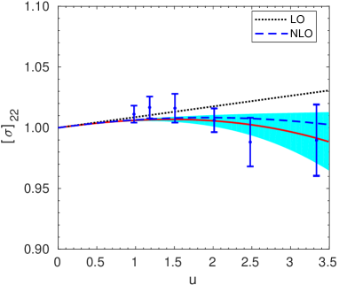
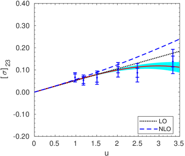
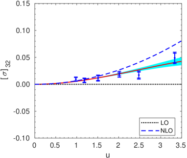
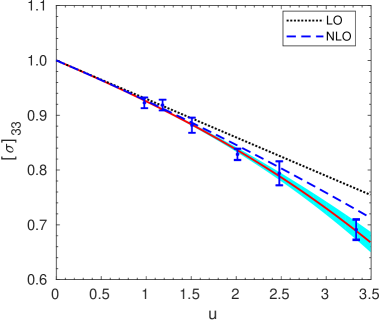
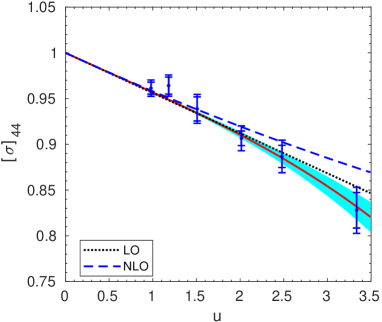
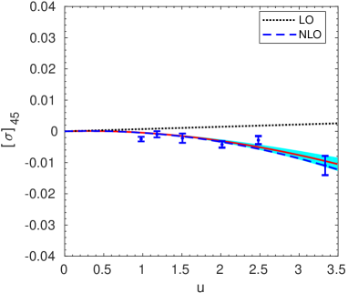
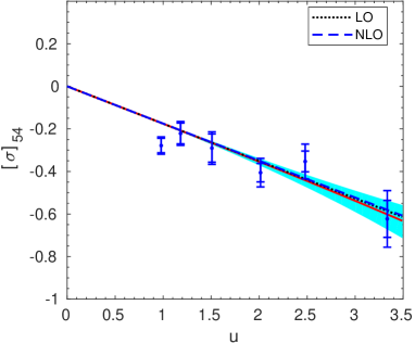
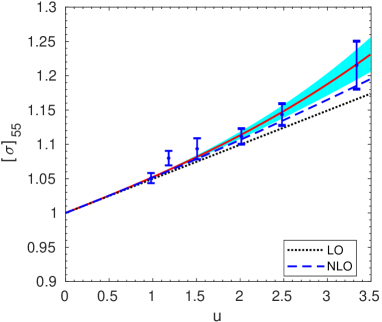
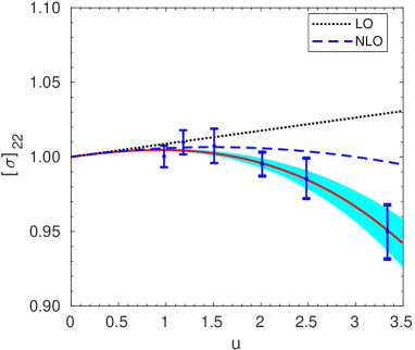
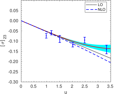
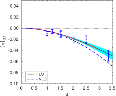
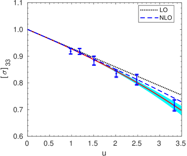
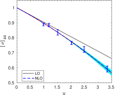
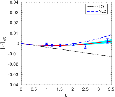
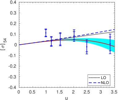
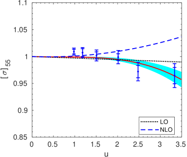
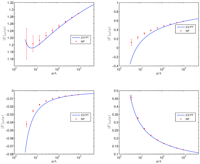
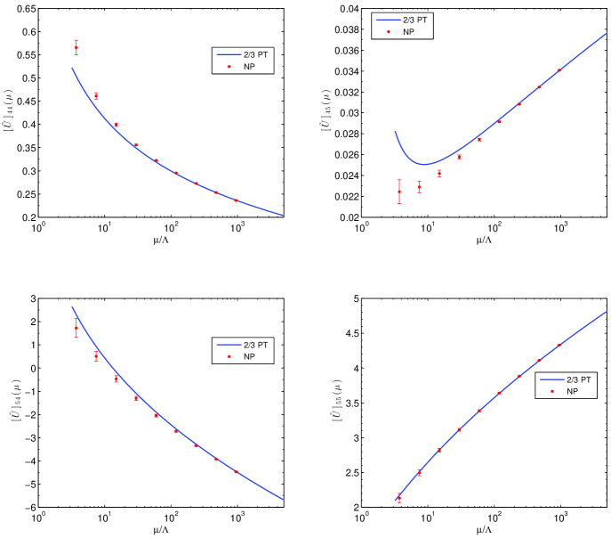
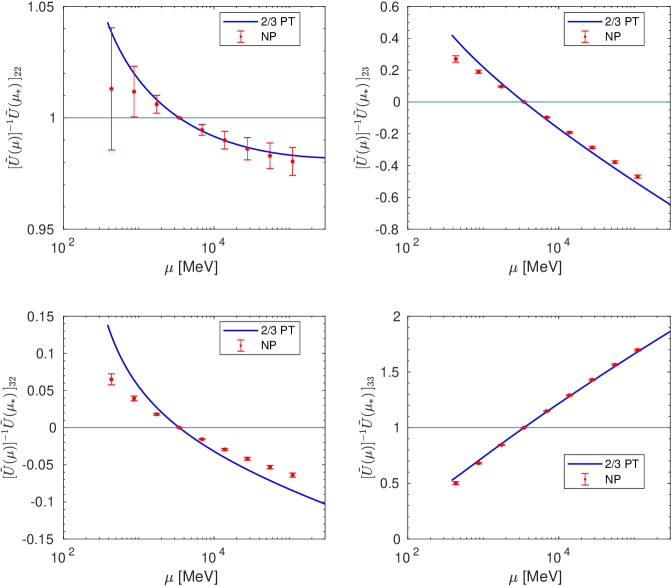
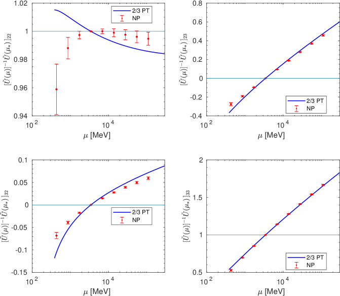
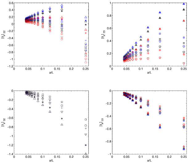
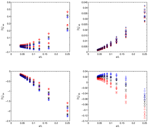
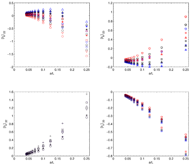
In order to compute the RG running of the operators in the continuum limit, matrix-SSFs have to be fit to the functional form shown in Eq. (3.78). Several fits have been tried out, with different orders in the polynomial expansion and either kept fixed to its perturbative value or allowed to be a free fit parameter. Fits with fixed by perturbation theory and the only free fit parameter do not describe the data well. This is understandable, as deviations from LO are large for some matrix elements (for in particular) and knowledge of the NLO anomalous dimension (and therefore ; cf. Eq. (3.87)) is necessary for a well-converging fit. It is however an encouraging crosscheck that the value returned by the fit is close to the perturbative prediction of Eq. (3.87). If, besides , we also include as a free fit parameter, the results have large errors. The best option turns out to be the one with the polynomial expansion of Eq. (3.78) truncated at , and fixed to their perturbative values and left as free fit parameter. The plots of the matrix-SSFs are collected in Figs. 2 and 3.
In the same Figures we also show the LO and NLO perturbative results, calculated from Eq. (3.78), truncated at and respectively. The comparison between the non-perturbative, the LO, and the NLO results provides a useful assessment of the reliability of the perturbative series. There is coincidence of all three curves at very small (perturbative) values of the squared gauge coupling , but this is obviously guaranteed by the form of our fit function, as described above. At larger -values one would ideally hope to see the NLO curves lying closer to the non-perturbative ones, compared to the LO curves. For this is mostly the case, as shown in Fig. 2, the only exception being and . For the operator basis , non-perturbative and NLO curves seem in good agreement for the diagonal elements and . This is less so for the non-diagonal and . For the operator basis , non-perturbative and NLO curves mostly agree, with the exception of . We also note that the non-perturbative tends to decrease at large , unlike the monotonically increasing perturbative predictions. For the NLO curves lie closer to the non-perturbative results compared to the LO ones, in all cases but and (for LO and NLO are very close to each other). In several cases non-perturbative and NLO curves are in fair, or even excellent, agreement also at large -values (cf. , , and ). In other cases this comparison in less satisfactory. Note that the NLO and curves are monotonically increasing, as opposed to the non-perturbative ones. In conclusion the overall picture in the renormalisation scheme under investigation is in accordance with our general expectations, although there are signs of slow or bad convergence of the perturbative results to the non-perturbative ones.
Once the matrix-SSFs are known as continuum functions of the renormalised coupling, we can obtain the RG-running matrix ; cf. Eq. (3.68). We check the reliability of our results by writing Eq. (2.35) as
| (4.91) |
The matrix does not depend on the higher-energy scale , so the -dependence on the rhs should in principle cancel out. We check this by computing the second line for varying , using our non-perturbative result for and the perturbative one for . As explained in the comments following Eq. (3.69), the latter is obtained as the NLO-2/3PT , multiplied by . The scale is held fixed through , which defines ; see the running coupling computation of ref. [19] for details. The higher-energy scale is varied over a range of values ; for each of these is computed. Our results are shown in Tabs. 3 and 4. As expected, -independence sets in with increasing .
More specifically, taking from ref. [19] and from ref. [15] with , we obtain the hadronic matching energy scale . Our final results for the non-perturbative running at are obtained from Eq. (4.91) and for . They are:
| (4.92) | |||||
| (4.93) |
for the operator bases , and
| (4.94) | |||||
| (4.95) |
for ,. The first error refers to the statistical uncertainty, while the second is the systematic one due to the use of NLO-2/3PT at the higher scale . We estimate the systematic error as the difference between the final result, obtained with perturbation theory setting in at scale , and the one where perturbation theory sets in at (cf. Tabs. 3,4).
We note that systematic errors are almost negligible compared to statistical ones, the latter being the result of error propagation in the product of matrix-SSFs from to . This however does not tell us much about the accuracy of NLO-2/3PT around the scale . We investigate this issue in Appendix A, where we compare , calculated in NLO-2/3PT and non-perturbatively. For several matrix elements of we see that NLO-2/3PT is not precise enough, even at the largest scale we can reach (corresponding to ).
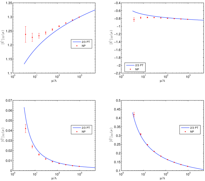
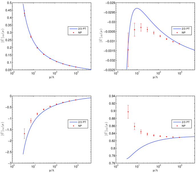
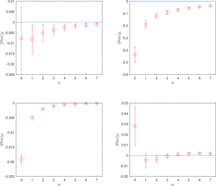
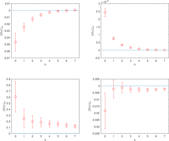
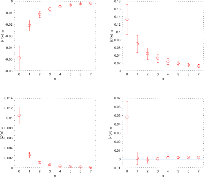
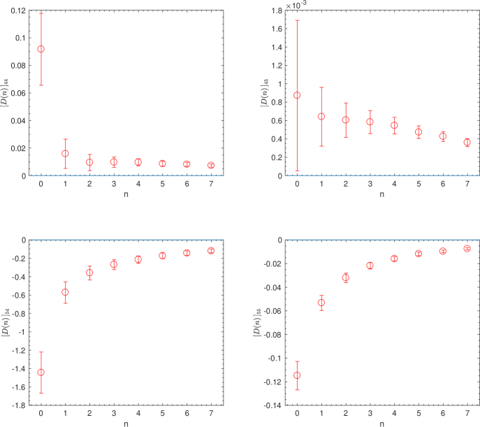
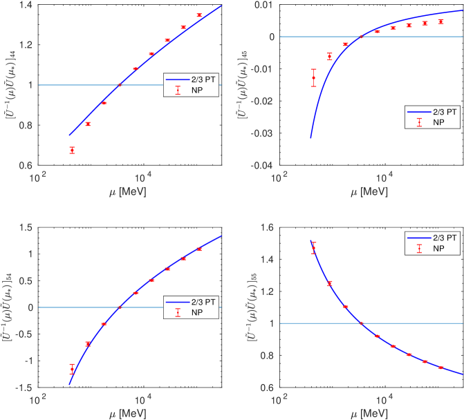
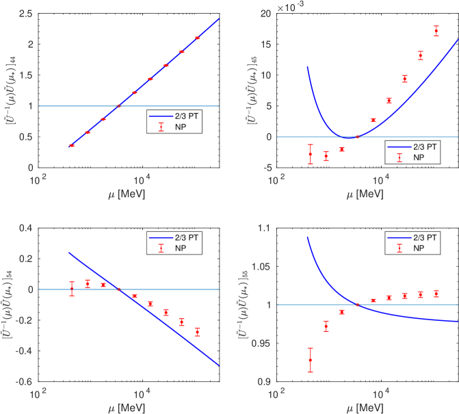
We now play the inverse game, keeping fixed and calculating
| (4.96) |
for decreasing . The results for are shown in Figs. 4 and 5. They are the first non-perturbative computation of the RG-evolution of operators which mix under renormalisation in the continuum. We stress that these results are scheme dependent. Note that the computation thus described enforces the coincidence of our most perturbative point to the perturbative prediction, which we assume to describe accurately the running from to infinity. The discrepancies between perturbation theory and our results are evident at ever decreasing scales . These discrepancies are sometimes dramatic; e.g. . This is related to the discussion of Figs. 2 and 3 above, concerning disagreements between non-perturbative and NLO behaviour of several matrix elements. Since in Eq. (4.96) is a product of several matrices, these disagreements accumulate, becoming very sizeable as decreases.
Finally, we compare the perturbative (NLO-2/3PT) to the non-perturbative RG evolution between scales and , where GeV is kept fixed and is varied in the range [0.43 GeV, 110 GeV]. The comparison is described Appendix A and confirms the unreliability of the perturbative computation of the RG running at scales of about .
| 0 | ||
| 1 | ||
| 2 | ||
| 3 | ||
| 4 | ||
| 5 | ||
| 6 | ||
| 7 | ||
| 8 |
| 0 | ||
| 1 | ||
| 2 | ||
| 3 | ||
| 4 | ||
| 5 | ||
| 6 | ||
| 7 | ||
| 8 |
4.3 Matching to hadronic observables with non-perturbatively improved Wilson fermions
Having computed the non-perturbative evolution matrices as in Eq. (4.96), which provide the RG-running at the low energy scale , we proceed to establish the connection between bare lattice operators and their RGI counterparts. Starting from the definition of Eq. (2.41), we write the RGI operator as
is independent of any renormalisation scheme or scale; of course it is also independent of the regularisation. It is a product of several quantities:
-
•
The factors and depend on a high-energy scale and are calculated in NLO perturbation theory. This was one of the main objectives of ref. [2].
-
•
The running matrix is known between the high-energy scale and a low-energy scale ; its non-perturbative computation for QCD is the main objective of the present work.
-
•
The product of the last two factors stands for the usual lattice computation of bare hadronic quantities and their renormalisation constants on large physical volumes and for several bare couplings, with the continuum limit taken though extrapolation.
Although the last item in the above list is beyond the scope of this paper, we have computed following [19], at three values of the lattice spacing, namely , which are in the range commonly used for simulations of QCD in physically large volumes. The results are listed in Tabs. 5, 6. In order to interpolate to the target renormalized coupling , the data can be fitted with a polynomial. Our numerical studies reveal that additional values of would be needed to improve the quality of the interpolation to the target value of the coupling.
| 5.20 | 0.13600 | 4 | 3.65 | ||
| 6 | 4.61 | ||||
| 5.29 | 0.13641 | 4 | 3.39 | ||
| 6 | 4.30 | ||||
| 8 | 5.65 | ||||
| 5.40 | 0.13669 | 4 | 3.19 | ||
| 6 | 3.86 | ||||
| 8 | 4.75 |
| 5.20 | 0.13600 | 4 | 3.65 | ||
| 6 | 4.61 | ||||
| 5.29 | 0.13641 | 4 | 3.39 | ||
| 6 | 4.30 | ||||
| 8 | 5.65 | ||||
| 5.40 | 0.13669 | 4 | 3.19 | ||
| 6 | 3.86 | ||||
| 8 | 4.75 |
5 Conclusions
In the present work we have studied the non-perturbative RG-running of the parity-odd, dimension-six, four-fermion operators , defined in Eqs. (2.6) and (2.7). Assigning physical flavours to the generic fermion fields , the above operators describe four-quark effective interactions for various physical processes at low energies. Under renormalisation, these operators mix in pairs, as discussed in Section 2. This mixing is not an artefact of the eventual loss of symmetry due to the (lattice) regularisation; rather it is a general property of operators belonging to the same representations of their symmetry groups. It follows that also the RG-running of each operator is governed by two anomalous dimensions, and the corresponding RG-equations are imposed on evolution matrices. This makes the problem of RG-running more complicated than the cases of multiplicatively renormalised quantities, such as the quark masses or .
The novelty of the present work is that, using long-established finite-size scaling techniques and the Schrödinger Functional renormalisation conditions described in Section 3, we have computed the non-perturbative evolution matrices of these operators between widely varying low- and high-energy scales and for QCD with two dynamical flavours. Our results are shown in Figs. 4 and 5 and Eqs. (4.92) – (4.95). The accuracy of our results for the diagonal matrix elements ranges from 3% to 5%. The accuracy on the determination of the non-diagonal matrix elements ranges from as high as 3% to as poor as 60%. Clearly there is room for improvement. In our next project concerning the renormalisation and RG-running of the same operators for QCD with three dynamical flavours, we plan to introduce several novelties, which ought to improve the precision of our results significantly.
Perturbation theory is to be used for the RG-running for scales above . In our SF scheme the perturbative results at our disposal are NNLO (3-loops) for the Callan-Symanzik -function and NLO (2-loops) for the four-fermion operator anomalous dimensions. In Figs. 4 and 5 we see the presence of possibly relevant non-perturbative effects already at scales of about 3 GeV, where it is often assumed that beyond-LO perturbation theory converges well101010We have checked that other SF schemes, with different choices of and (see subsection 3.1), display similar overall behaviour.. We have also performed some checks by computing the RG-evolution matrix from a generic scale to a scale of about 3 GeV and found some matrix elements where the NLO perturbative result significantly differs from the non-perturbative one (see Appendix A). This should serve as a warning for other non-perturbative approaches which assume that perturbation theory is convergent at such scales.
Finally, at a fixed hadronic scale and for three values of the bare gauge coupling, we have computed the renormalisation constants (again in matrix form) of our four-fermion operators.
As a closing remark we wish to point out that the non-perturbative evolution matrices computed in this work describe not only the RG-running of the parity-odd operators , but also that of their parity-even counterparts . This is because evolution matrices are continuum quantities: in the continuum, each parity-odd operator combines with its parity-even counterpart to form an operator which transforms in a given chiral representation, both parts having consequently the same anomalous dimension matrices.
In the case, for instance, of transitions, we are dealing with operator matrix elements between two neutral -meson states and therefore only the parity-even operators ( in the SM and for BSM) contribute. Our results for the continuum RG-evolution, obtained for the parity-odd basis, can be used in this case. The renormalization of the bare operators, however, depends on the details of the lattice action. If the lattice regularisation respects chiral symmetry (e.g. lattice QCD with Ginsparg-Wilson fermions), then the parity-even and parity-odd parts of a given basis of chiral operators renormalise with the same renormalisation constants. Consequently they also have the same matrix-SSFs and evolution matrices. All results obtained for the parity-odd operators are then also valid for the , without further ado.
Things are somewhat more complicated if the regularisation breaks chiral symmetry (e.g. lattice QCD with Wilson fermions). Then parity-even and parity-odd operators again have the same anomalous dimensions, as these are continuum quantities, but the “ratio” of their renormalisation matrices is a finite (scale-independent) matrix which is a function of the bare gauge coupling; it becomes the unit matrix in the continuum limit. This “ratio” is fixed by lattice Ward identities, as discussed for example in ref. [7]. So the subtlety here is that once the renormalisation condition has been fixed for say, the parity-odd operator bases at a value of the squared gauge coupling, the condition for the parity-even counterparts is also fixed through . Consequently, renormalisation matrix “ratios” like are equal to their parity-even counterparts . Thus matrix-SSFs and evolution matrices are the same for parity-odd and parity-even cases; cf. Eq. (3.66). But if we wish to use the evolution matrices of the present work also for the parity-even operators, we must ensure that these are renormalised in the “same” SF scheme employed for their parity-odd counterparts. This is ensured by writing the RGI parity-even operator column (in analogy to Eq. (4.3)) as:
where is the “subtracted” bare operator, as suggested by Eq. (2.8). The term in square brackets of the last expression is the renormalised parity-even operator . It is computed however in a way that ensures that the bare operator is renormalised in our SF scheme: the SF renormalisation parameter (which removes the logarithmic divergences) is multiplied by the scheme-independent, scale-independent “ratio” .
Clearly, the procedure sketched above for the renormalisation of parity-even operators is fairly cumbersome. It is also prone to enhanced statistical uncertainties, as it involves subtracted operators with non-zero . Fortunately, there is a way to circumvent the problem: it is well known that, using chiral (axial) transformations of the quark fields, we can obtain continuum correlation functions of specific parity-even composite operators in terms of bare correlation functions of parity-odd operators of the same chiral multiplet, regularised with twisted-mass (tmQCD) Wilson fermions [23]. The prototype example is the one expressing renormalized correlation functions of the axial current in terms of bare twisted-mass Wilson-fermion correlation functions of the properly renormalised vector current. The situation is more complicated with four-fermion operators: in ref. [8] it was shown that such chiral rotations do indeed relate parity-even to parity-odd 4-fermion operators, but the resulting tmQCD Wilson-fermion determinant is not real, and thus unsuitable for numerical simulations. This problem is circumvented by working with a lattice theory with sea- and valence-quarks regularised with different lattice actions [9]. The valence action is the so-called Osterwalder-Seiler [24] variety of tmQCD, with valence twisted-mass fermion fields suitably chosen so as to enable the mapping of correlation functions involving parity-even operators to those of the parity-odd basis . The sea-quark action may be any tenable lattice fermion action. While the price to pay is the loss of unitarity at finite values of the lattice spacing, this is, however, outweighed by the advantage of vanishing finite subtractions ( in eq. (2.8)).
Acknowledgments
The present work is an extension of previous efforts dedicated to the SF renormalisation and running of the -parameter in the Standard Model. We are indebted to our collaborators at the time, namely M. Guagnelli, J. Heitger, F. Palombi, and S. Sint, for their early contributions. We owe a lot to their participation in the defining phase of this project. G.H., C.P. and D.P. acknowledge support by the Spanish MINECO grant FPA2015-68541-P (MINECO/FEDER), the MINECO’s Centro de Excelencia Severo Ochoa Programme under grant SEV-2016-0597 and the Ramón y Cajal Programme RYC-2012-10819. M.P. acknowledges partial support by the MIUR-PRIN grant 2010YJ2NYW and by the INFN SUMA project.
| 0.9793 | 9.50000 | 0.131532 | 6 | |||
| 9.73410 | 0.131305 | 8 | ||||
| 10.05755 | 0.131069 | 12 | ||||
| 1.1814 | 8.50000 | 0.132509 | 6 | |||
| 8.72230 | 0.132291 | 8 | ||||
| 8.99366 | 0.131975 | 12 | ||||
| 1.5078 | 7.54200 | 0.133705 | 6 | |||
| 7.72060 | 0.133497 | 8 | ||||
| 8.02599 | 0.133063 | 12 | ||||
| 2.0142 | 6.60850 | 0.135260 | 6 | |||
| 6.82170 | 0.134891 | 8 | ||||
| 7.09300 | 0.134432 | 12 | ||||
| 2.4792 | 6.13300 | 0.136110 | 6 | |||
| 6.32290 | 0.135767 | 8 | ||||
| 6.63164 | 0.135227 | 12 | ||||
| 3.3340 | 5.62150 | 0.136665 | 6 | |||
| 5.80970 | 0.136608 | 8 | ||||
| 6.11816 | 0.136139 | 12 |
A Non-perturbative vs perturbative behaviour of the RG evolution
In analogy to Appendix C of ref. [12] we construct the quantity:
| (A.99) | |||||
Once again , , and are perturbative quantities known in NLO-2/3PT , while is a single non-perturbative matrix-SSF. In the last line of Eq. (A.99), the product is the ratio of the non-perturbative over the perturbative RG evolution between scales and . If perturbation theory were reliable at these high scales, would vanish at large . The results for the matrix elements are shown in Figs. 10, 11. At the largest values some of them are compatible with 0 while others are not. The latter case signals that due to large anomalous dimensions, NLO-2/3PT performs poorly even at scales as high as and .
Moreover, in Appendix C of ref. [12] the non-perturbative RG evolution between scales and has been compared to the result from NLO-2/3PT. In ref. [12], is kept fixed to 2 GeV while is varied in the range [2 GeV, 3 GeV]. We perform a similar study by fixing the reference scale , corresponding to the squared coupling . This is the scale closest to the interval [2 GeV, 3 GeV] of ref. [12], for which we have directly computed the matrix-SSFs non-perturbatively. The scale is varied in the range [0.43 GeV, 110 GeV]. We compute in the following way:
| (A.100) | |||||
can be evaluated in a purely non-pertubative way for integer and . The results are presented Figs. 12, 13. Very dominant non-perturbative effects are clearly visible for the elements , , and of the operators and . Given the large deviation from the NLO-2/3PT running already seen in Fig. 5, these results are not surprising and simply confirm the non-reliability of the NLO-2/3PT computation of the RG running at scales around . Notice that the scale interval where this comparison has been performed in ref. [12] is completely contained in our plots between the third and the fourth point which correspond to scales of 1.73 GeV and 3.46 GeV. We remind the reader that a direct comparison between our results and those of ref. [12] is meaningless, the crucial differences being, among many others, the renormalisation scheme and the -value.
B One-loop cutoff effects in the step scaling function
In Tab. 9 we gather numerical values for , defined in Eq. (3.76). We have calculated this quantity for a fermionic action with () and without () a Clover term. These results are also displayed in Figs. 14, 15, 16, and 17 (the target scheme , is plotted with a blue triangle). Notice that the element of is independent from due to an accidental cancellation. This is why all data-points in the corresponding figures are not in colour. As expected, the Clover term has an important effect on the discretisation errors, which are significantly reduced when . The observed discretisation effects in Figs. 14 and 15 are only due to the unimproved operators, the action being tree-level improved.
References
- [1] ALPHA Collaboration, P. Dimopoulos, G. Herdoiza, F. Palombi, M. Papinutto, C. Pena, and A. Vladikas, Non-perturbative renormalisation of four-fermion operators in two-flavour QCD, JHEP 0805 (2008) 065, [0712.2429].
- [2] M. Papinutto, C. Pena, and D. Preti, On the perturbative renormalization of four-quark operators for new physics, Eur. Phys. J. C77 (2017), no. 6 376, [1612.06461].
- [3] S. Aoki et. al., Review of lattice results concerning low-energy particle physics, Eur. Phys. J. C77 (2017), no. 2 112, [1607.00299].
- [4] F. Palombi, C. Pena, and S. Sint, A Perturbative study of two four-quark operators in finite volume renormalization schemes, JHEP 03 (2006) 089, [hep-lat/0505003].
- [5] ALPHA Collaboration, M. Guagnelli, J. Heitger, C. Pena, S. Sint, and A. Vladikas, Non-perturbative renormalization of left-left four-fermion operators in quenched lattice QCD, JHEP 03 (2006) 088, [hep-lat/0505002].
- [6] P. Dimopoulos, L. Giusti, P. Hernández, F. Palombi, C. Pena, A. Vladikas, H. Wennekers, and H. Wittig, Non-perturbative renormalisation of left-left four-fermion operators with Neuberger fermions, Phys.Lett. B641 (2006) 118–124, [hep-lat/0607028].
- [7] A. Donini, V. Giménez, G. Martinelli, M. Talevi, and A. Vladikas, Nonperturbative renormalization of lattice four fermion operators without power subtractions, Eur. Phys. J. C10 (1999) 121–142, [hep-lat/9902030].
- [8] C. Pena, S. Sint, and A. Vladikas, Twisted mass QCD and lattice approaches to the rule, JHEP 0409 (2004) 069, [hep-lat/0405028].
- [9] R. Frezzotti and G. Rossi, Chirally improving Wilson fermions. II. Four-quark operators, JHEP 0410 (2004) 070, [hep-lat/0407002].
- [10] M. Ciuchini, E. Franco, V. Lubicz, G. Martinelli, I. Scimemi, et. al., Next-to-leading order QCD corrections to effective Hamiltonians, Nucl.Phys. B523 (1998) 501–525, [hep-ph/9711402].
- [11] A. Buras, M. Misiak, and J. Urban, Two loop QCD anomalous dimensions of flavor changing four quark operators within and beyond the standard model, Nucl.Phys. B586 (2000) 397–426, [hep-ph/0005183].
- [12] RBC, UKQCD Collaboration, P. A. Boyle, N. Garron, R. J. Hudspith, C. Lehner, and A. T. Lytle, Neutral kaon mixing beyond the Standard Model with nf = 2 + 1 chiral fermions. Part 2: non perturbative renormalisation of the four-quark operators, JHEP 10 (2017) 054, [1708.03552].
- [13] M. Lüscher, S. Sint, R. Sommer, and P. Weisz, Chiral symmetry and improvement in lattice QCD, Nucl. Phys. B478 (1996) 365–400, [hep-lat/9605038].
- [14] S. Capitani, M. Lüscher, R. Sommer, and H. Wittig, Non-perturbative quark mass renormalization in quenched lattice QCD, Nucl. Phys. B544 (1999) 669–698, [hep-lat/9810063]. [Erratum: Nucl. Phys.B582,762(2000)].
- [15] ALPHA Collaboration, M. Della Morte, R. Frezzotti, J. Heitger, J. Rolf, R. Sommer, and U. Wolff, Computation of the strong coupling in QCD with two dynamical flavors, Nucl. Phys. B713 (2005) 378–406, [hep-lat/0411025].
- [16] ALPHA Collaboration, S. Sint and P. Weisz, The Running quark mass in the SF scheme and its two loop anomalous dimension, Nucl. Phys. B545 (1999) 529–542, [hep-lat/9808013].
- [17] M. Luscher, R. Sommer, U. Wolff, and P. Weisz, Computation of the running coupling in the SU(2) Yang-Mills theory, Nucl. Phys. B389 (1993) 247–264, [hep-lat/9207010].
- [18] ALPHA Collaboration, K. Jansen and R. Sommer, O() improvement of lattice QCD with two flavors of Wilson quarks, Nucl. Phys. B530 (1998) 185–203, [hep-lat/9803017]. [Erratum: Nucl. Phys.B643,517(2002)].
- [19] ALPHA Collaboration, M. Della Morte, R. Hoffmann, F. Knechtli, J. Rolf, R. Sommer, I. Wetzorke, and U. Wolff, Non-perturbative quark mass renormalization in two-flavor QCD, Nucl. Phys. B729 (2005) 117–134, [hep-lat/0507035].
- [20] M. Lüscher, R. Narayanan, P. Weisz, and U. Wolff, The Schrödinger functional: A Renormalizable probe for nonAbelian gauge theories, Nucl. Phys. B384 (1992) 168–228, [hep-lat/9207009].
- [21] ALPHA Collaboration, A. Bode, P. Weisz, and U. Wolff, Two loop computation of the Schrodinger functional in lattice QCD, Nucl. Phys. B576 (2000) 517–539, [hep-lat/9911018]. [Erratum: Nucl. Phys.B600,453(2001)].
- [22] ALPHA Collaboration, U. Wolff, Monte Carlo errors with less errors, Comput. Phys. Commun. 156 (2004) 143–153, [hep-lat/0306017]. [Erratum: Comput. Phys. Commun.176,383(2007)].
- [23] Alpha Collaboration, R. Frezzotti, P. A. Grassi, S. Sint, and P. Weisz, Lattice QCD with a chirally twisted mass term, JHEP 08 (2001) 058, [hep-lat/0101001].
- [24] K. Osterwalder and E. Seiler, Gauge Field Theories on the Lattice, Annals Phys. 110 (1978) 440.