Mind-to-mind heteroclinic coordination:
model of sequential episodic memory initiation

Abstract

Retrieval of episodic memory is a dynamical process in the large scale brain networks. In social groups, the neural patterns, associated to specific events directly experienced by single members, are encoded, recalled and shared by all participants. Here we construct and study the dynamical model for the formation and maintaining of episodic memory in small ensembles of interacting minds We prove that the unconventional dynamical attractor of this process – the nonsmooth heteroclinic torus – is structurally stable within the Lotka-Volterra-like sets of equations. Dynamics on this torus combines absence of chaos with asymptotic instability of every separate trajectory; its adequate quantitative characteristics are length-related Lyapunov exponents. Variation of the coupling strength between the participants results in different types of sequential switching between metastable states; we interpret them as stages in formation and modification of the episodic memory.

Our ability to graft images and ideas into the minds of other humans is crucial for the existence of science, technology and literature. Participation of a community member in an event or group of events (episode) suffices to implant the memory of that episode into the minds of the whole community. In our daily life we take this ability for granted, but only the recent advances of measurement technique have disclosed how e.g., a movie spectator encodes and transfers aposteriori to listeners the neural patterns associated with viewing specific episodes, and how these event-specific patterns are shared among the brains. In the large-scale networks of the individual brain, a retrieval of episodic memory occurs in a way of sequential switching between the events, the perpetual “winnerless competition”. We propose and investigate the mathematical model for the formation and maintaining of common memory in interacting minds. By combining rigorous proofs with numerical studies we show that weak coupling between the participant’s minds ensures the existence of the so-called “attracting heteroclinic torus” in the phase space of the model. Changing the coupling strength, we observe different types of dynamics that correspond to various forms of episodic memory.

I Introduction

Even across different languages, our brains show similar activity, or become ”aligned” when we hear the same idea or story. This amazing neural mechanism allows us to transmit brain patterns, sharing memories and knowledge.
                                                    Uri Hasson (2016).

Development of technology and science, as well as the sheer existence of oral and written literature owes much to the fact that personal participation in an event is not a necessary precondition of keeping that event in one’s memory: humans are able to mentally construct episodes when reading or listening to recollections of other humans. A recent study, based on analysis of magnetic resonance brain imaging during the performance of verbal communication tasks, traced how neural patterns associated with viewing specific scenes in a movie were encoded, recalled, and then transferred to a group of listeners who had not seen the movie Zadbood_2017 . It disclosed that event-specific patterns, observed in the brain default mode network, were shared across the processes of encoding, recall, and construction of the same episodes. Such studies uncover intimate correspondences between episodic memory encoding and construction, and underscore the role of the common language in the transmission of memory to other brains.

Communication in persistent social groups (families, friends, colleagues, $\ldots$) is facilitated by common episodic memories: interpersonal knowledge of past, shared by the group members Bietti_2010 . Distributed within the group, such memories serve as a stem around which new layers of shareable information are accumulated. Notably, episodic memories are not exact replicas of the lives: rather, they are organized summaries of experience, encoded in the form of sequential groups of events Heusser_2017 . According to recent imaging data, the brain areas responsible for storage and retrieval of episodic memories include hippocampus, striatum and the prefrontal cortex Sadeh_2011 ; Collin_2017 .

Low-dimensional mind dynamics

Below, we present and study a low-dimensional model of mind-to-mind episodic memory interaction. We emphasize from the beginning that we intend not to model the brain itself as a system but to create a dynamical model for the activity of this system. Our ultimate goal is to describe, understand and make predictions of mind dynamics, obtaining, in particular, dynamical models of specific classes of such activities as cognition, creativity, and autobiographic memory.

Recent technological progress has allowed the researchers to observe the brain patterns with resolution and clearness that could be previously only dreamed of. The prominent role is currently played by functional magnetic resonance imaging (fMRI) that tracks the changes associated with the blood flow through the brain. Experimental findings indicate that cognition in the human brain, as well as the conscience of certain mammals:
a) is closer to determinism than to random processes;
b) bears the characteristic features of low-dimensional dynamics, and
c) manifests itself in the form of sequential metastable spatio-temporal patterns.

We cite just a few pertinent publications:

• In a recent study, Ma and Zhang investigate the temporal organization of resting-state functional connectivity (RSFC) in awake rodents and humans. They report: “We found that transitions between RSFC patterns were not random but followed specific sequential orders. Transitions between RSFC patterns exhibited high reproducibility and were significantly above chance”, and conclude: “Spontaneous brain activity is not only nonrandom spatially, but also nonrandom temporally” Ma_Zhang_2018 .

• By analyzing local field potentials from the cortices of rats under anesthesia, Hudson et al. find out that “recovery of consciousness occurs after the brain traverses a series of metastable intermediate activity configurations” Hudson_et_al_2014 . They demonstrate that “recovery is confined to a low-dimensional subspace” and conclude that “organization of metastable states, along with dramatic dimensionality reduction, significantly simplifies the task of sampling the parameter space” Hudson_et_al_2014 .

• Analysis of high temporal resolution human fMRI data from a large sample of unrelated individuals in the study of Shine et al Shine_Breakspear_2017 suggests that the “integrative core of brain regions … manipulates the low-dimensional architecture of the brain across an attractor landscape via highly conserved modulatory neurotransmitter systems”; reconstruction of state-space trajectories unambiguously confirms “existence of a low-dimensional, dynamic, integrated component that recurs across multiple unique tasks and demarcates a common cognitive architecture within the human brain”. The authors of the study summarize: “Global brain states exist along a low dimensional manifold” Shine_Breakspear_2017 .

• In the study Slapsinskaite_2017 of incremental exhaustive cycling performed by the group of physically active adults, the participants were instructed to monitor bodily regions with discomfort and pain. Tracking the evolution of pain-attention during the exercises, the researchers disclosed the “dynamical phenomenon of chunking that the biological-cognitive system uses to manage larger sequence of information into smaller units to facilitate information processing”; they concluded that “the chunks operate on an heteroclinic cycle of metastable states where each metastable state itself is a heteroclinic cycle of basic information items”.

• Finally, experimental studies on the formation of episodic memory Baldassano_et_al_2017 show how “cortical structures generate event representations during narrative perception and how these events are stored to and retrieved from memory. The data-driven approach allows to detect event boundaries as shifts between stable patterns of brain activity without relying on stimulus annotations and reveals a nested hierarchy from short events in sensory regions to long events in high order areas (including angular gyrus and posterior medial cortex), which represent abstract, multimodal situation models.” Below, we interpret such “shifts” as heteroclinic switches between metastable patterns.

In accordance with this convincing evidence, certain kinds of mind activity definitely can be (and already are) a subject for low-dimensional dynamical modeling Friston_2000 ; Tognoli_Kelso_2014 ; Cocchi_et_al_2017 .

Our modeling approach below is based on the following assumptions, suggested by experimental data:

1. Sensory, semantic and emotional information is encoded, memorized, stored and retrieved by global brain networks.

2. During perception, encoded patterns are similar for different humans that share memory representations for the same real-life events Chen_2017 .

3. In the course of continuous perception, the brain automatically segments experience into discrete events Baldassano_2017 , “the meaningful segments of one’s life, the coherent units of one’s personal history” Beal_Weiss_2013 . Segmented information is memorized in the form of abstract patterns at the high level of hippocampus and cortical areas Chen_2017 .

4. Memorized events are segmented into chunks chunking_2014 . Temporally organized chunks form episodes, organized into sequences changing with environment Cohn_Sheehy_Ranganath_2017 .

5. Recent studies provide evidence that within events, temporal memory is related to temporal stability of brain memory patterns Clewett_Davachi_2017 . Accordingly, in the phase space the event patterns should display metastability: In the retrieval process the chunks compete and form heteroclinic chains of sequentially switching metastable patterns Rabinovich_2008 ; Rabinovich_2015 ; Bick_and_Rabinovich_2009 .

These assumptions lead us to the simplified dynamical model of the mutual mind-to-mind interaction. We demonstrate that the attractor of the model in the case of two interacting subsystems (brains) for a wide range of parameters is the unconventional object: the two-dimensional non-smooth invariant torus. Peculiarity of dynamics upon it is strict absence of chaos, contrasted with instability (in the sense of Lyapunov) of each trajectory. Remarkably, the proper characteristics of the instability are not the conventional Lyapunov exponents (average rates of instability growth per time unit), but the average rates of instability growth per unit of orbit length in the phase space. At larger strength of the coupling between the partners, the torus undergoes a breakup, and the resulting dynamical pattern indicates some kind of cooperative interaction, akin to synchronization in certain features, but different from it in the other ones.

The layout of the paper is as follows. In Sect.II, starting from general requirements to characteristics of individual brain dynamics and to kinds of interactions between the brains, we delineate the class of considered dynamical systems and reduce it to a set of coupled units, each one governed by Lotka-Volterra-like ordinary differential equations. Each subsystem features the non-autonomous episodic memory recall; mathematically, we interpret it as the closed heteroclinic chain of episodes in the long term memory under parametric excitation by sequences that come from the partner subsystems.

The bulk of the paper is focused on the simplest case: unidirectional mind-to-mind entrainment, “master-slave” dynamics. In Section III we show that the attractor of this system is the two-dimensional non-smooth invariant torus. When subsystems are uncoupled, this torus appears as the direct product of two heteroclinic cycles, and, as we rigorously prove, it persists at least under sufficiently small coupling strength. Every trajectory on the torus is a heteroclinic connection joining two metastable states of equilibrium. Hence, dynamics on the torus is absolutely non-chaotic. Nevertheless, as numerical experiments in Sect.IV force us to believe, each trajectory in the basin of this attractor is Lyapunov unstable. When, at stronger coupling, the torus breaks up, dynamics in the slaved subsystem turns into alternation of piecewise constant segments that follows the switches in the master subsystem.

II The basic model of social cooperation

Dynamical cell assembly coding belongs to prevailing concepts in the context of information processing in the individual human brain. In global functional brain networks these assemblies form different spatio-temporal modes. When the minds interact, specific networks are responsible for the performance of specific cognitive functions in the partners. Since the coding occurs on the population level, dynamics of the modes is usually low-dimensional Ma_Zhang_2018 . Low-dimensionality results from coherent activity of many elements that form modes, and can be extracted from the records by application of e.g., principal component analysis Hudson_et_al_2014 ; Shine_Breakspear_2017 . We assume that $N$ different spatio-temporal patterns (brain modes) $P_{i}(\vec{r},t),\;i=1,2,\ldots,N$ are characterized by a discrete set of spatial coordinates $\vec{r}$. Spatial structure of the patterns is influenced, besides physiological factors, by the social environment. Noteworthy, $P_{i}(\vec{r},t)$ may have different sense, related to the performance of different cognitive and behavioral tasks.

The patterns $P_{i}(\vec{r},t)$ can be based on several brain subnetworks like perceptual, memory, and motor brain circuits, therefore their intrinsic dynamics can be quite complex. In certain cases, temporal and spatial patterns of the modes can be separated: $P_{i}(\vec{r},t)=Q_{i}(\vec{r})\,R_{i}(t)$ where $Q_{i}(\vec{r})$ describes the spatial organization of the $i$-th mode and $R_{i}(t)$ characterizes its temporal evolution. Remarkably, the amplitudes $R_{i}$ cannot be initiated “from outside”: the mode, absent at a particular moment of time, will be absent for all subsequent times. Suppose that all $R_{i}(t)$ obey a kinetic equation up to the second order. If, as the result of the inferential process, the spatial structure of the modes is known, then, after factorization, the basic kinetic model for a single brain can be written in the generalized Lotka-Volterra form:

$$\dot{R}_{i}=R_{i}\big{(}\overline{\sigma}_{i}-R_{i}-\sum_{j\neq i}^{N}\overline{\rho}_{ij}R_{j}\big{)}+\varepsilon\zeta_{i}(R_{i}),\,i=1,\ldots,N.$$ (1)

Here $\overline{\sigma}_{i}$ denotes the excitation rate of the $i$-th mode, $\{\overline{\rho}_{ij}\}$ is the cognitive inhibition matrix that characterizes the mutual interaction between the modes, and $\varepsilon$ parameterizes the environmental state-dependent fluctuations $\zeta_{i}$.

Below we describe the interaction between two social partners; generalization to larger number of participants is straightforward. Denote the temporal patterns $R_{i}(t)$ for partners $X$ and $Y$ by the sets of functions $x_{i}(t)$ ($i$=$1,\ldots,N_{x}$) and $y_{s}(t)$ ($s$=$1,\ldots,N_{y}$) respectively. In general, each mode of $X$ should be enabled to interact with every mode of $Y$ and vice versa. Then, collective dynamics is governed by the system

$$\dot{x}_{i} = x_{i}\left(\sigma_{i}-x_{i}-\sum_{j\neq i}^{N_{x}}\rho_{ij}x_{j}\,-q\sum_{s=1}^{N_{y}}\theta_{is}y_{s}\right)+\varepsilon\zeta_{i}(x_{i})$$

$$\dot{y}_{k} = y_{k}\left(\delta_{k}-y_{k}-\sum_{k\neq s}^{N_{y}}\xi_{ks}y_{s}\,-p\sum_{s=1}^{N_{x}}\eta_{ks}x_{s}\right)+\varepsilon\overline{\zeta}_{k}(y_{k})$$

where $\sigma_{i}$ and $\delta_{k}$ are the respective sets of excitation rates for the participants $X$ and $Y$, $\{\rho_{ij}\}$ and $\{\xi_{ks}\}$ are their cognitive inhibition matrices, the parameters $p$ and $q$ measure the strength of the social interaction, and the interaction itself is prescribed by the matrices $\{\theta_{is}\}$ and $\{\eta_{ks}\}$. Finally, $\zeta_{i}$ and $\tilde{\zeta}_{k}$ are state-dependent fluctuations (noise) that will be specified below.

Formally, the system (II) is just the decomposition of (1). However, our setup distinguishes between the patterns formed by $X$ and those formed by $Y$. Accordingly, we expect that the largest elements in the matrices $\rho,\,\xi,\,\theta,\,\eta$ are of the order one whereas the coupling coefficients $p$ and $q$ stay relatively small.

II.1 Configurations of social entrainment

Complex dynamics of the system (II) in the wide domains of parameter values is able to represent the evolution of the sequences of events/episodes. It is thereby a convenient model for the analysis of mutual social influence on the performance of episodic memory. In different regions of its parameter space, various attractors can be encountered; for example, many of the 64 stationary solutions (states of equilibrium) are stable in certain parameter ranges. We are, however, not interested in stable equilibria or in simple limit cycles: episodic memory, as it is known from the experiments, is neither time-independent, nor strictly periodic. Hence we seek in the parameter space the domains where all states of equilibrium are unstable nodes or saddle points. Presence of many invariant hyperplanes in the phase space favors formation of structurally (within the frame of Lotka-Volterra-like systems) stable heteroclinic connections between the saddle points. In the context of the memory functioning, such connections enable an efficient dynamical way of information coding through robust sequential switching, based on the winnerless competition principle. The image of this coding in the phase space is the stable heteroclinic channel (see Fig. 1 ).

  

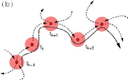
Figure 1: (a) Global brain network whose activity can be represented in the cognitive space by robust sequential switching; excitation level of different network modes is shown by different colors (b) Stable heteroclinic channel with a chain of metastable states (informational patterns). Dashed lines: separatrices of metastable states (Adapted from Varona_Rabinovich_2016 ).

In our mathematical and numerical studies below, we restrict ourselves to the minimal configuration with $N_{x}$=$N_{y}$=3: operating with just three patterns for each of two partners delivers a revealing example of heteroclinic switching in the mind-to-mind dynamics. Cases of larger $N_{x}$ and $N_{y}$, albeit more demanding computationally, can be treated in the similar way.

If the information exchange between the participants is unidirectional ($|q|\ll|p|$) – this happens, for example, if $X$ does not focus her/his attention on the visual or verbal signals of $Y$ – the model (II) allows for simplification, enabling the analytic investigation.

Purely unidirectional connection acquires importance in yet another situation, relevant for the modeling of memory-related processes. Suppose the brain $X$ is not the brain of some other person but it is the brain of $Y$ in the past. Then the stated problem turns into the question, how the episodic memory from the past encodes memory dynamics for the future: a dynamical description of the imagination process. Several decades ago, D. Ingvar recognized: in order to be useful, a simulation of the future event should be encoded into memory so that the gained information can be retrieved at a later time when the simulated behavior is actually carried out; he termed this process “memory of the future” Ingvar_1985 (for further details see Szpunar_2013 ; Schacter_2017 ). From the dynamical theory point of view, “memory of the future” is a result of the inhibitory interaction of the events-modes from the past episodic memory with modes in the present time (see Varona_Rabinovich_2016 ). About the role of memory inhibition in imagination of the sequences see Gomez-Ariza_2017 .

This setup differs from heteroclinic harmonic entrainment, observed in the single three-state network under sinusoidal forcing Rabinovich_et_al_2006 : The localized in time actions of information units are determined not only by the frequency of heteroclinic cycling but also by the characteristics (exit times) of metastable states.

II.2 Dynamical characteristics: length-related Lyapunov exponents.

When characterizing dynamical regimes in the model (II), we cannot rely on the standard tools like conventional Lyapunov exponents: in the situation of heteroclinicity to states of equilibrium, they are of little help. Recall that the Lyapunov exponents are defined for the reference trajectory in the system of order $N$ as

$$\lambda_{i}=\lim_{t\to\infty}\frac{1}{t}\log\frac{\|\tilde{x}_{i}(t)\|}{\|\tilde{x}_{i}(0)\|},\;\;i=1,\dots N,$$ (3)

where $\tilde{x}_{i}(t)$ are linearly independent solutions of the linearization near this reference trajectory, that start from $N$ appropriate perturbation vectors $\tilde{x}_{i}(0)$. In our case, we expect that the largest $\lambda_{i}$ vanish and cannot help us to measure the amount of instability stored in the attraction basin.

This can be explained by the following reasoning. A conventional Lyapunov exponent characterizes the rate of perturbation growth per unit of time. For trajectories close to heteroclinicity and their perturbations tangent to invariant hyperplanes in the phase space of (II), the overwhelming (asymptotically tending to 1) proportion of time is spent in nearly static configurations, hence a characterization in terms of time units loses its merits. A more appropriate characteristics of weak instability in this situation requires a different parameterization of the trajectory: the rate of perturbation growth per unit of length of the reference trajectory in the phase space,

$$\Lambda_{i}=\lim_{t\to\infty}\frac{1}{L(t)}\log\frac{\|\tilde{x}_{i}(t)\|}{\|\tilde{x}_{i}(0)\|},\;\;i=1,\dots N,$$ (4)

where $L(t)$ is the (Euclidean) length of the segment of the reference phase trajectory between time instants 0 and $t$. This kind of characteristics was introduced in  AN where the standard (time-related) Lyapunov exponent vanished for similar reasons whereas the length-related ones were positive. For the numerical example treated below in Section IV, in a range of coupling strength there are two positive length-related exponents $\Lambda_{1,2}$ and, hence, $\|\tilde{x}_{1,2}(t)\|\sim\exp\big{(}\Lambda_{1,2}L(t)\big{)}$. Recalling that dynamics with two or more positive $\lambda_{i}$ is termed “hyperchaos”, here we can speak of weak hyperchaos.

The length-related Lyapunov exponents not only quantify this kind of dynamics but also serve as indicators of essential transitions: in our context, bifurcations of the torus break-up. In the exemplary system treated in Section IV, such bifurcations occur due to the partial regain of stability by equilibria belonging to the attractor: their formerly two-dimensional unstable manifolds become one-dimensional. After this event, only one length-related Lyapunov exponent stays positive. Accordingly, dynamics becomes “one-dimensional” but in a tricky way: time plots of observables are almost piecewise constant, with each plateau corresponding to the interval of activity for one of the master variables (see details below).

III Non-smooth torus: rigorous results

Here, we introduce and study a new dynamical object: two dimensional non-smooth invariant torus $\mathbb{T}^{2}$ that can be viewed as a mathematical image of interactions, in the master-slave way, of two cognitive systems.

When the systems are uncoupled, this object appears as the direct product of two heteroclinic cycles, and, as we prove below, it persists at least under small rates of coupling. Since every trajectory on $\mathbb{T}^{2}$ is a heteroclinic connection between two saddle points, dynamics upon it cannot be chaotic. Nevertheless, as follows from numerical experiments in the subsequent Sect. IV, each trajectory in the basin of this attractor is Lyapunov unstable. Thus, we deal here with a situation, quite different both from the case of chaotic attractors and from the phenomenon of transient chaos where instability of trajectories is caused by the presence of an unstable chaotic set in the boundary of the attractors basin GOY . For the first time, dynamics of this kind was reported in AN : a numerical study of interaction between two systems, one of them possessing a heteroclinic cycle and another one having a stable limit cycle ACY . Two-dimensional sets, entirely consisting of heteroclinic connections, were studied also in  ARF and  AMY but instability of trajectories in the basin of attractor was out of scope of those publications.

In this Section, we treat the variant of the system (II) with unilateral coupling and without fluctuating terms:

$$\dot{x}_{i} = x_{i}\big{(}\sigma_{i}-x_{i}-\sum_{j\neq i}\rho_{ij}x_{j}\big{)}$$ (5)

$$\dot{y}_{k} = y_{k}\big{(}\delta_{k}-y_{k}-\sum_{s\neq k}\xi_{ks}y_{s}-p\sum_{s=1}^{3}\eta_{ks}x_{s}\big{)}$$ (6)

where $\sigma_{i}>0$, $\rho_{ij}>0$, $\delta_{k}>0$, $\xi_{ks}>0$, $\eta_{ks}\geq 0$,   $i,j,k,s\in\{1,2,3\}$.

III.1 The uncoupled system

Our analysis refers to small values of the coupling strength $p$. We begin with the decoupled case

$$\dot{x}_{i} = x_{i}(\sigma_{i}-x_{i}-\sum_{j\neq i}\rho_{ij}x_{j}),\hskip 17.07182pti,j=1,2,3$$ (7)

$$\dot{y}_{k} = y_{k}(\delta_{k}-y_{k}-\sum_{s\neq k}\xi_{ks}y_{s}),\hskip 17.07182ptk,s=1,2,3.$$ (8)

First, we impose conditions under which subsystem (7) has a heteroclinic cycle AZR . This system has altogether 8 states of equilibrium. Of these, three states lie on the coordinate axes. These are $O_{1}=(\sigma_{1},0,0)$, $O_{2}=(0,\sigma_{2},0)$, $O_{3}=(0,0,\sigma_{3})$ with eigenvalues equal to

$$\sigma_{2}-\rho_{21}\sigma_{1},\; \sigma_{3}-\rho_{31}\sigma_{1}, -\sigma_{1}\hskip 14.22636pt\text{at}\hskip 5.69046ptO_{1},$$

$$\sigma_{3}-\rho_{32}\sigma_{2},\; \sigma_{1}-\rho_{12}\sigma_{2},\, -\sigma_{2}\hskip 14.22636pt\text{at}\hskip 5.69046ptO_{2},\hskip 14.22636pt\text{and}$$

$$\sigma_{1}-\rho_{13}\sigma_{3},\; \sigma_{2}-\rho_{23}\sigma_{3}, -\sigma_{3}\hskip 14.22636pt\text{at}\hskip 5.69046ptO_{3}.$$

Under the conditions

$$\sigma_{2}-\rho_{21}\sigma_{1}>0, \sigma_{3}-\rho_{31}\sigma_{1}<0,$$

$$\sigma_{3}-\rho_{32}\sigma_{2}>0, \sigma_{1}-\rho_{12}\sigma_{2}<0,$$ (9)

$$\sigma_{1}-\rho_{13}\sigma_{3}>0, \sigma_{2}-\rho_{23}\sigma_{3}<0.$$

every $O_{i}$ ($i$=1,2,3) has the one-dimensional unstable and the two-dimensional stable manifolds.

Moreover, if $\rho_{21}\rho_{12}\neq 1,\;\rho_{32}\rho_{23}\neq 1$, and $\rho_{13}\rho_{31}\neq 1,$ the unstable manifold of $O_{i}$ contains a heteroclinic trajectory $\Gamma_{i,(i\,\rm{mod}\,3)+1}$ joining $O_{i}$ and $O_{(i\,\rm{mod}\,3)+1}$. Under a combination of all these conditions, the system (7) has a heteroclinic cycle

$$\Gamma=\cup_{i}O_{i}\cup_{i}\Gamma_{(i\,\rm{mod}\,3)+1}$$

For the sake of definiteness, we assume that the leading direction on the stable manifold of $O_{i}$ is different from the coordinate axis, i.e.,

$$-\sigma_{1} < \sigma_{3}-\rho_{31}\sigma_{1},$$

$$-\sigma_{2} < \sigma_{1}-\rho_{12}\sigma_{2},$$ (10)

$$-\sigma_{3} < \sigma_{2}-\rho_{23}\sigma_{3}.$$

Then, the heteroclinic cycle has a shape sketched in Fig. 2a.

1

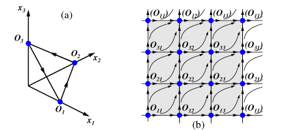
Figure 2: (a) The heteroclinic cycle $\Gamma$; (b) Unfolding of the torus $T_{0}$ on the plane: sketch of the vector field.

Finally, we impose stability conditions

$$-\frac{(\sigma_{3}-\rho_{31}\sigma_{1})}{\sigma_{2}-\rho_{21}\sigma_{1}} > 1,$$

$$-\frac{(\sigma_{1}-\rho_{32}\sigma_{2})}{\sigma_{3}-\rho_{32}\sigma_{2}} > 1,$$ (11)

$$-\frac{(\sigma_{2}-\rho_{23}\sigma_{3})}{\sigma_{1}-\rho_{13}\sigma_{3}} > 1,$$

under which $\Gamma$ is attracting.

Similarly, for the subsystem (8) we consider three equilibrium points $\tilde{O}_{1}=(\delta_{1},0,0)$, $\tilde{O}_{2}=(0,\delta_{2},0)$, $\tilde{O}_{3}=(0,0,\delta_{3})$ and impose:

1. Conditions for the existence of one-dimensional unstable and two-dimensional stable manifolds at $\tilde{O}_{i}$:

   $$\delta_{2}-\xi_{21}\delta_{1}>0, \quad\delta_{3}-\xi_{31}\delta_{1}<0,$$

   $$\delta_{3}-\xi_{32}\delta_{2}>0, \quad\delta_{1}-\xi_{12}\delta_{2}<0,$$ (12)

   $$\delta_{1}-\xi_{13}\delta_{3}>0, \quad\delta_{2}-\xi_{23}\delta_{3}<0.$$

2. Conditions for leading directions:
   

   $$-\delta_{1} < \delta_{3}-\xi_{31}\delta_{1},$$

   $$-\delta_{2} < \delta_{1}-\xi_{12}\delta_{2},$$ (13)

   $$-\delta_{3} < \delta_{2}-\xi_{23}\delta_{3}.$$

3. Conditions for the existence of heteroclinic trajectories: $\xi_{21}\xi_{12}\neq 1,\quad\xi_{32}\xi_{23}\neq 1,\quad\xi_{13}\xi_{31}\neq 1.$

4. Conditions of stability:

   $$-\frac{(\delta_{3}-\xi_{31}\delta_{1})}{\delta_{2}-\xi_{21}\delta_{1}}>1, \displaystyle-\frac{(\delta_{1}-\xi_{32}\delta_{2})}{\delta_{3}-\xi_{32}\delta_{2}}>1, -\frac{(\delta_{2}-\xi_{23}\delta_{3})}{\delta_{1}-\xi_{13}\delta_{3}}>1.$$

Under these provisions, subsystem (8) has an attractor

$$\tilde{\Gamma}=\cup_{i=1}^{3}\tilde{O}_{i}\cup_{i}\tilde{\Gamma}_{(i\,\rm{mod}\,3)+1},$$

where $\tilde{\Gamma}_{(i\,\rm{mod}\,3)+1}$ is the heteroclinic trajectory joining $\tilde{O}_{i}$ and $\tilde{O}_{(i\,\rm{mod}\,3)+1}$. The heteroclinic cycle $\tilde{\Gamma}$ looks analogously to $\Gamma$ in Fig. 2a.

Hence, it follows that the system (7,8) has an invariant set $T_{0}$ that is the direct product of $\Gamma$ and $\tilde{\Gamma}$: $T_{0}=\Gamma\times\tilde{\Gamma}$. Since both $\Gamma$ and $\tilde{\Gamma}$ are homeomorphic to the circle, $T_{0}$ is homeomorphic to the two-dimensional torus $\mathbb{T}^{2}$. The equilibrium points belonging to $T_{0}$ are $O_{ij}=O_{i}\times\tilde{O}_{j}$; the eigenvalues of the linearized at these points system (7,8) are summarized in the Table 1.

Saddle	Eigenvalues
$O_{11}$	$-\sigma_{1}$, $\sigma_{2}-\rho_{21}\sigma_{1}$, $\sigma_{3}-\rho_{31}\sigma_{1}$, $-\delta_{1}$, $\delta_{2}-\xi_{21}\delta_{1}$, $\delta_{3}-\xi_{31}\delta_{1}$
$O_{12}$	$-\sigma_{1}$, $\sigma_{2}-\rho_{21}\sigma_{1}$, $\sigma_{3}-\rho_{31}\sigma_{1}$, $-\delta_{2}$, $\delta_{3}-\xi_{32}\delta_{2}$, $\delta_{1}-\xi_{12}\delta_{2}$
$O_{13}$	$-\sigma_{1}$, $\sigma_{2}-\rho_{21}\sigma_{1}$, $\sigma_{3}-\rho_{31}\sigma_{1}$, $-\delta_{3}$, $\delta_{1}-\xi_{13}\delta_{3}$, $\delta_{2}-\xi_{23}\delta_{3}$
$O_{21}$	$-\sigma_{2}$, $\sigma_{3}-\rho_{32}\sigma_{2}$, $\sigma_{1}-\rho_{31}\sigma_{1}$, $-\delta_{1}$, $\delta_{2}-\xi_{21}\delta_{1}$, $\delta_{3}-\xi_{31}\delta_{1}$
$O_{22}$	$-\sigma_{2}$, $\sigma_{3}-\rho_{32}\sigma_{2}$, $\sigma_{1}-\rho_{12}\sigma_{2}$, $-\delta_{2}$, $\delta_{3}-\xi_{32}\delta_{2}$, $\delta_{1}-\xi_{12}\delta_{2}$
$O_{23}$	$-\sigma_{2}$, $\sigma_{3}-\rho_{32}\sigma_{2}$, $\sigma_{1}-\rho_{12}\sigma_{2}$, $-\delta_{3}$, $\delta_{1}-\xi_{13}\delta_{3}$, $\delta_{2}-\xi_{23}\delta_{3}$
$O_{31}$	$-\sigma_{3}$, $\sigma_{1}-\rho_{13}\sigma_{3}$, $\sigma_{1}-\rho_{23}\sigma_{3}$, $-\delta_{1}$, $\delta_{2}-\xi_{21}\delta_{1}$, $\delta_{3}-\xi_{31}\delta_{1}$
$O_{32}$	$-\sigma_{3}$, $\sigma_{1}-\rho_{13}\sigma_{3}$, $\sigma_{2}-\rho_{23}\sigma_{3}$, $-\delta_{2}$, $\delta_{3}-\xi_{32}\delta_{2}$, $\delta_{1}-\xi_{12}\delta_{2}$
$O_{33}$	$-\sigma_{3}$, $\sigma_{1}-\rho_{13}\sigma_{3}$, $\sigma_{2}-\rho_{23}\sigma_{3}$, $-\delta_{3}$, $\delta_{1}-\xi_{13}\delta_{3}$, $\delta_{2}-\xi_{23}\delta_{3}$

Table 1: Eigenvalues of the linearized system (7,8).

The assumed conditions imply that each of the points $O_{ij}$ has the two-dimensional unstable manifold and the four-dimensional stable manifold (below we denote these manifolds by, respectively, $W^{u}$ and $W^{s}$). Moreover, some of $O_{ij}$ are joined by heteroclinic trajectories. To list them we introduce the following notation: let $H(A\rightarrow B)$ be a heteroclinic trajectory joining the equilibrium points A and B. For heteroclinic cycles $\Gamma$ and $\tilde{\Gamma}$ we have the heteroclinic trajectories: $H(O_{1}\rightarrow O_{2})=:\Gamma_{12}$, $H(O_{2}\rightarrow O_{3})=:\Gamma_{23}$, $H(O_{3}\rightarrow O_{1})=:\Gamma_{31}$, $H(\tilde{O}_{1}\rightarrow\tilde{O}_{2})=:\tilde{\Gamma}_{12}$, $H(\tilde{O}_{2}\rightarrow\tilde{O}_{3})=:\tilde{\Gamma}_{23}$, and $H(\tilde{O}_{3}\rightarrow\tilde{O}_{1})=:\tilde{\Gamma}_{31}$. Heteroclinic trajectories can be listed in the way presented in the Table 2.

$O_{1}$	$H(O_{11}\to O_{12})=O_{1}\times\tilde{\Gamma}_{12}$	$H(O_{12}\to O_{13})=O_{1}\times\tilde{\Gamma}_{23}$	$H(O_{13}\to O_{11})=O_{1}\times\tilde{\Gamma}_{31}$
$O_{2}$	$H(O_{21}\to O_{22})=O_{2}\times\tilde{\Gamma}_{12}$	$H(O_{22}\to O_{23})=O_{2}\times\tilde{\Gamma}_{23}$	$H(O_{23}\to O_{21})=O_{2}\times\tilde{\Gamma}_{31}$
$O_{3}$	$H(O_{31}\to O_{32})=O_{3}\times\tilde{\Gamma}_{12}$	$H(O_{32}\to O_{33})=O_{3}\times\tilde{\Gamma}_{23}$	$H(O_{33}\to O_{31})=O_{3}\times\tilde{\Gamma}_{31}$
$\tilde{O}_{1}$	$H(O_{11}\to O_{21})=\Gamma_{12}\times\tilde{O}_{1}$	$H(O_{21}\to O_{31})=\Gamma_{23}\times\tilde{O}_{1}$	$H(O_{31}\to O_{11})=\Gamma_{31}\times\tilde{O}_{1}$
$\tilde{O}_{2}$	$H(O_{12}\to O_{22})=\Gamma_{12}\times\tilde{O}_{2}$	$H(O_{22}\to O_{32})=\Gamma_{23}\times\tilde{O}_{2}$	$H(O_{32}\to O_{12})=\Gamma_{31}\times\tilde{O}_{2}$
$\tilde{O}_{3}$	$H(O_{13}\to O_{23})=\Gamma_{12}\times\tilde{O}_{3}$	$H(O_{23}\to O_{33})=\Gamma_{23}\times\tilde{O}_{3}$	$H(O_{33}\to O_{13})=\Gamma_{31}\times\tilde{O}_{3}$

Table 2: Heteroclinic trajectories of basic heteroclinic network of $T_{0}$.

For convenience, we place in the left column of this Table the equilibrium points that enter the corresponding direct products. These 18 heteroclinic trajectories form a basic heteroclinic network: see Fig. 3.

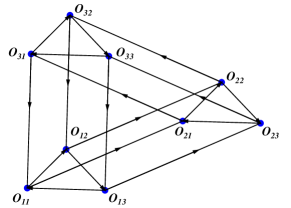
Figure 3: Heteroclinic network $\Gamma_{0}$ on the torus $T_{0}$.

Let us now construct a two-dimensional invariant surface for which $\Gamma_{0}$ plays the role of ”skeleton”. For that, we show that each ”rectangle” in $\Gamma_{0}$ serves as a boundary of a two-dimensional invariant surface. Consider, e.g., the rectangle formed by the heteroclinic trajectories $H(O_{13}\rightarrow O_{11})$, $H(O_{31}\rightarrow O_{11})$, $H(O_{33}\rightarrow O_{31})$, $H(O_{33}\rightarrow O_{13})$ and the points $O_{33}$, $O_{31}$, $O_{13}$, $O_{11}$. All these heteroclinic trajectories and saddle points belong to the four-dimensional invariant plane $x_{2}=y_{2}=O$ which we denote by $\mathbb{R}^{4}$.

Recalling that $H(O_{13}\rightarrow O_{11})=O_{1}\times\tilde{\Gamma}_{31}$, $H(O_{33}\rightarrow O_{31})=O_{3}\times\tilde{\Gamma}_{31}$ and $H(O_{31}\rightarrow O_{11})=\Gamma_{31}\times\tilde{O}_{1}$, $H(O_{33}\rightarrow O_{13})=\Gamma_{31}\times\tilde{O}_{3}$, we naturally consider the two-dimensional surface $\Gamma_{31}\times\tilde{\Gamma}_{31}=\tilde{R}_{0}$ that possesses the following properties:

1. It is invariant by definition.

2. $\tilde{R}_{0}\subset\mathbb{R}^{4}$, by definition.

3. $\tilde{R}_{0}\subset{W^{u}}_{O_{33}}$. Indeed, a point in $\tilde{R}_{0}$ is the product of two points, say P $\in\Gamma_{31}$ and $Q\in\tilde{\Gamma}_{31}$. As time goes to $-\infty$, the representative point on $\Gamma_{31}$ tends to $O_{3}$ and that on $\tilde{\Gamma}_{3}$ tends to $\tilde{O}_{3}$, so the representative point the trajectory of the full system going through $P\times Q$ tends to $O_{33}$.

4. $\tilde{R}_{0}\subset{W^{s}}_{O_{11}}$. The proof is the same as in (iii). Thereby, $\tilde{R}_{0}$ is a collection of heteroclinic connections joining $O_{33}$ and $O_{11}$, see Fig 4.

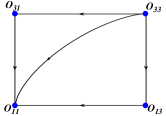
Figure 4: The rectangle $\tilde{R}_{0}$.

In the same way we prove that there are other 8 rectangles with boundaries consisting of heteroclinic trajectories from the basic network, see Fig 3. They form a two-dimensional surface, say, $T_{0}$, homeomorphic to the two-dimensional torus. In fact, $T_{0}$ is the direct product of heteroclinic cycles in the systems (7) and (8).

By construction, the complete set of trajectories on $T_{0}$ consists of nine metastable equilibria $O_{ij}$ and heteroclinic connections joining them pairwise. Since in the full phase space of system (7,8) all $O_{ij}$ are structurally stable saddles, their presence on the toroidal surface (in absence of compensating nodes or foci) may seem to violate the index theorem. However, reduction to $T_{0}$ involves “folding” along the separatrices of the saddles. As seen in the schematic unfolding of $T_{0}$ on the two-dimensional plane sketched in Fig. 2b, the procedure of folding turns steady states into compound equlibria: in the adjacent segment of the plane, each of them is a source in one quadrant, a sink in another one and a saddle point in two remaining quadrants, so that the resulting Poincaré index of every steady state is identically zero. Accordingly, the total index of $T_{0}$ vanishes as well, as required for every two-dimensional toroidal surface.

Now we formulate the sufficient conditions under which $T_{0}$ is an attractor. For that, we remind the notion of the saddle index Sh . If $O$ is a hyperbolic saddle point with Jacobian eigenvalues $\lambda_{1},\dots,\lambda_{m}$, $\gamma_{1},\dots,\gamma_{n}$ such that $\operatorname{Re}{\lambda_{i}}<0$, $\operatorname{Re}{\gamma_{j}}>0$, then the number

$$\nu=-\frac{\max_{i}\operatorname{Re}\lambda_{i}}{\max_{j}\operatorname{Re}\gamma_{j}}$$

is called the saddle index of $O$. If $\nu>1$, the point $O$ is called the dissipative saddle. For example, for the point $O_{33}$ the saddle index equals

$$\nu=-\frac{\max\{\sigma_{2}-\rho_{23}\sigma_{3},\delta_{2}-\xi_{23}\delta_{3}\}}{\max\{\sigma_{1}-\rho_{13}\sigma_{3},\delta_{1}-\xi_{13}\delta_{3}\}}$$

See Table 1 and the inequalities (III.1) - ((ii).).

Theorem 1.

If all saddle points in $\Gamma_{0}$ are dissipative, then $T_{0}$ is an attractor.

Proof.

It suffices to show that the representative point on the trajectory passing through any initial point in a neighborhood of $T_{0}$ tends to $T_{0}$ as $t\rightarrow\infty$. Without a loss of generality we start with an initial point $q_{0}$ that is close to one of the equilibria in $\Gamma_{0}$; let this equilibrium be, e.g., $O_{33}$. Let $\epsilon={\rm dist}(q_{0},{W_{O}^{s}}_{33})$. It follows (see Sh ; AH ) that the orbit passing through $q_{0}$ leaves a neighborhood of $O_{33}$ at a point $q_{1}$ such that ${\rm dist}(q_{1},{W_{O}^{u}}_{33})<\epsilon^{\nu_{0}}$ where $1<\nu_{0}<\nu_{33}$ ($\nu_{33}$ denotes the saddle index of $O_{33}$). Then the orbit follows a trajectory on ${W_{O}^{u}}_{33}$ and comes, after a finite time, to a point $q_{2}$ in a small neighborhood of the equilibrium $\tilde{O}$ that is either $O_{33}$ or $O_{13}$ or $O_{11}$, so that ${\rm dist}(q_{3},W^{s}(\tilde{O}))<C\epsilon^{\nu_{0}}$, $C=const$. If $\epsilon$ has been small enough, then $C\epsilon^{\nu_{0}}<\epsilon/2$. Then we reproduce the previous consideration for the point $\tilde{O}$, replacing $\epsilon$ by $\epsilon/2$. Repeating this procedure again and again, we ensure that ${\rm dist}(q_{2k+1},T_{0})<{\epsilon}/{2^{k}}$ where $q_{2k+1}$ is the representative point after the time in which the trajectory intersects $k$ successive neighborhoods. Remark that we should choose constant $C$ only finitely many times independently of $k$ since the passage time from one neighborhood of an equilibrium to another one in the same rectangle is bounded from above. Thus, the representative point tends to $T_{0}$ as $t\rightarrow+\infty$. ∎

Table 3 shows the saddle indices of all saddles in $\Gamma_{0}$.

Saddle	Saddle index $\nu$
$O_{11}$	$\frac{-\max\{\sigma_{3}-\rho_{31}\sigma_{1},\delta_{3}-\xi_{31}\delta_{1}\}}{\max\{\sigma_{2}-\rho_{21}\sigma_{1},\delta_{2}-\xi_{21}\delta_{1}\}}$
$O_{12}$	$\frac{-\max\{\sigma_{3}-\rho_{31}\sigma_{1},\delta_{1}-\xi_{12}\delta_{2}\}}{\max\{\sigma_{2}-\rho_{21}\sigma_{1},\delta_{3}-\xi_{32}\delta_{2}\}}$
$O_{13}$	$\frac{-\max\{\sigma_{3}-\rho_{31}\sigma_{1},\delta_{2}-\xi_{23}\delta_{3}\}}{\max\{\sigma_{2}-\rho_{21}\sigma_{1},\delta_{1}-\xi_{13}\delta_{3}\}}$
$O_{21}$	$\frac{-\max\{\sigma_{1}-\rho_{12}\sigma_{2},\delta_{3}-\xi_{31}\delta_{1}\}}{\max\{\sigma_{3}-\rho_{32}\sigma_{2},\delta_{2}-\xi_{21}\delta_{1}\}}$
$O_{22}$	$\frac{-\max\{\sigma_{1}-\rho_{12}\sigma_{2},\delta_{1}-\xi_{12}\delta_{2}\}}{\max\{\sigma_{3}-\rho_{32}\sigma_{2},\delta_{3}-\xi_{32}\delta_{3}\}}$
$O_{23}$	$\frac{-\max\{\sigma_{1}-\rho_{12}\sigma_{2},\delta_{2}-\xi_{23}\delta_{3}\}}{\max\{\sigma_{3}-\rho_{32}\sigma_{2},\delta_{1}-\xi_{13}\delta_{3}\}}$
$O_{31}$	$\frac{-\max\{\sigma_{2}-\rho_{23}\sigma_{3},\delta_{3}-\xi_{31}\delta_{1}\}}{\max\{\sigma_{1}-\rho_{13}\sigma_{3},\delta_{2}-\xi_{21}\delta_{1}\}}$
$O_{32}$	$\frac{-\max\{\sigma_{3}-\rho_{23}\sigma_{3},\delta_{1}-\xi_{12}\delta_{2}\}}{\max\{\sigma_{1}-\rho_{13}\sigma_{3},\delta_{3}-\xi_{32}\delta_{2}\}}$

Table 3: Saddle indices of the saddle equilibrium points.

III.2 Persistence of $\Gamma_{0}$ and $T_{0}$ for small values of $|p|$

Now we introduce in Eq.(8) the weak non-zero coupling $p$ from the subsystem $X$ to the subsystem $Y$.

1. Persistence of $\Gamma_{0}$
   To show the persistence of the heteroclinic network $\Gamma_{0}$ we consider all heteroclinic orbits belonging to it. Without loss of generality we choose the rectangle $\tilde{R}_{0}$; the proof for other rectangles is similar.

   Persistence of $H(O_{33}\rightarrow O_{31})=O_{1}\times\tilde{\Gamma}_{31}$.
   This trajectory belongs to the three dimensional plane $x_{2}=x_{3}=0$, $y_{2}=0$. Denote it by $\mathbb{R}^{3}_{1}$. This plane is invariant for $\varepsilon=0$ both for the system (7,8) and (5,6). Inside $\mathbb{R}^{3}_{1}$ the point $O_{33}=(\sigma_{1},0,\delta_{3})$ is the saddle equilibrium point for the system (7,8) with eigenvalues $-\sigma_{1}$, $\delta_{1}-\xi_{13}\delta_{3}$, $\delta_{2}-\xi_{23}\delta_{3}$, see ((i).), i.e., with one-dimensional unstable manifold whereas the point $O_{31}=(\sigma_{1},0,\delta_{1})$ is the stable node with eigenvalues $-\sigma_{1}$, $-\delta_{1}$, $\delta_{3}-\xi_{31}\delta_{1}$, see Table 1. Inside $\mathbb{R}^{3}_{1}$, for small values of $|p|$ the saddle (node) equilibrium point stays the saddle (node). Denote them by $O_{33}(p)$ and $O_{31}(p)$. The smooth dependence of the unstable manifold on parameters and continuous dependence of solutions of the ODE on parameters imply that for small values of $|p|$ there exists a heteroclinic orbit joining $O_{33}(p)$ and $O_{31}(p)$. Persistence of this heteroclinic trajectory is a structurally stable feature.

   Persistence of $H(O_{33}\rightarrow O_{13})=\Gamma_{31}\times\tilde{O}_{3}$.
   This trajectory belongs to the three-dimensional invariant plane $x_{2}=0$, $y_{1}=y_{2}=0$, say $\mathbb{R}^{3}_{2}$. Inside $\mathbb{R}^{3}_{2}$ the point $O_{33}=(0,\sigma_{3},\delta_{3})$ is the saddle with the eigenvalues $\sigma_{1}-\rho_{13}\sigma_{3}$, $\sigma_{2}-\rho_{23}\sigma_{3}$, $-\delta_{3}$, and the point $O_{13}=(\sigma_{1},0,\delta_{3})$ is the node with the eigenvalues $-\sigma_{1}$, $\sigma_{3}-\rho_{31}\sigma_{1}$, $-\delta_{3}$, The situation is structurally stable as well.

   Persistence of $H(O_{31}\rightarrow O_{11})=\Gamma_{31}\times\tilde{O}_{1}$.
   This trajectory belongs to the three-dimensional invariant plane $x_{2}=0$, $y_{2}=y_{3}=0$, say $\mathbb{R}^{3}_{3}$. Inside $\mathbb{R}^{3}_{3}$ (which is invariant also for $p\neq 0$) the point $O_{31}=(\sigma_{3},0,\delta_{1})$ is the saddle with the eigenvalues $-\sigma_{3}$, $\sigma_{1}-\rho_{13}\sigma_{3}$, $-\delta_{1}$, and the point $O_{11}$ is the node with the eigenvalues $-\sigma_{1}$, $\sigma_{3}-\rho_{31}\sigma_{1}$, $-\delta_{1}$. The heteroclinic trajectory joining $O_{31}$ and $O_{11}$ inside $\mathbb{R}^{3}_{3}$ is also structurally stable.

   Persistence of $H(O_{13}\rightarrow O_{11})=O_{1}\times\tilde{\Gamma}_{31}$.
   The heteroclinic trajectory belongs to the three-dimensional invariant plane $x_{2}=x_{3}=0$, $y_{2}=0$, say $\mathbb{R}^{3}_{4}$. Inside it the point $O_{13}=(\sigma_{1},0,\delta_{3})$ is the saddle with the eigenvalues $-\sigma_{1}$, $\delta_{1}-\xi_{13}\delta_{3}$, $-\delta_{3}$, and $O_{11}$ is the node, with the eigenvalues $-\sigma_{1}$, $-\delta_{1}$, $\delta_{3}-\xi_{31}\delta_{1}$. Again, persistence of this trajectory is a structurally stable property.

   Summarizing, we conclude:

   Theorem 2.

   Under the above conditions the heteroclinic network $\Gamma_{0}$ persists for sufficiently small values of $|p|$.

2. Persistence of the heteroclinic attractor

   To show the existence of a heteroclinic attractor at weak coupling $|p|$, we prove the persistence of all rectangles that form $T_{0}$. As an example, we take the rectangle $\tilde{R_{0}}$; for other rectangles the proof is similar. The proof is based on the following facts,

   1. All points $O_{ij}(p)$ belong to the invariant four-dimensional space $\mathbb{R}^{4}_{0}$ $(x_{2}=y_{2}=0)$. At small values of $|p|$, they are saddle points in $\mathbb{R}_{4}$ with two-dimensional unstable manifolds. Heteroclinic trajectories between them that exist for small $|p|$ due to Theorem 2, also belong to $\mathbb{R}^{4}_{0}$. Denote them by $\Gamma_{ij}(p)$, so that $\Gamma_{ij}(0)=\Gamma_{ij}$, $i,j\in\{1,2,3\}$.

   2. At $p=0$, the point $O_{11}$ is the stable node in $\mathbb{R}^{4}_{0}$ with negative eigenvalues $-\sigma_{1}$, $-\delta_{1}$, $\sigma_{3}-\rho_{31}\delta_{1}$, $\delta_{3}-\xi_{31}\delta_{1}$, all of them disjoint from zero. Hence, at small values of $|p|$ it is still a sink, and there exists an absorbing region $U$ with the maximal attractor $O_{11}$ inside it: see Fig 5.

      

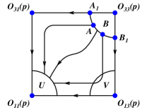
      Figure 5: Trajectories on the rectangle.

   3. The local unstable manifold of $O_{33}(p)$ depends smoothly on parameters, so for small values of $|p|$ it is $C^{1}$ close to $W^{u}(O_{33}(0))$, the local unstable manifold for $p$=0. Therefore, if one chooses an initial point $q$ on the interval $(A,B)$, Fig. 5, on $W^{u}(O_{33}(p))$ it will be close to a point $q_{0}\in W^{u}(O_{33}(0))$. For the uncoupled system ($p=0$) the trajectory passing through $q_{0}$ reaches $U$ in finite, bounded from above time. Thus, the trajectory of the system (5,6) passing through $q$ also comes into $U$ in finite time if $|p|$ is small enough.

   4. We show now that the representative point on the trajectory passing through a point $\tilde{q}\in(A,A_{1})\cup(B,B_{1})$ comes eventually into $U$. Without loss of generality we may assume that the point $B$ is so close to $B_{1}$ that the trajectory passing through it intersects a small neighborhood $V$ of $O_{13}(p)$ at a point $\tilde{q}_{1}$ such that ${\rm dist}(\tilde{q}_{1},W^{u}(O_{13}(p))<\delta$. We apply now the known results (see e.g., the book Sh ) to establish that ${\rm dist}(\tilde{q}_{2},W^{u}(O_{13}(p))<\delta^{\nu}$ where $\tilde{q}_{2}$ is the point on the considered trajectory at the instant when it leaves $V$ (see Fig. 6) and $1<\nu<\nu_{13}$, $\nu_{13}$ is the saddle index of $O_{13}(p)$.

      

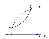
      Figure 6: Trajectories in $V$.

      This means that if $\delta$ is small enough, then the point $\tilde{q}_{2}$ is close to a point on the heteroclinic trajectory joining $O_{13}(p)$ and $O_{11}(p)$, therefore the trajectory passing through $\tilde{q}_{2}$ reaches $U$ in finite time. The proof for points on $(A,A_{1})$ is the same.

   5. Thus, we have proved that every trajectory passing though a point on $(A_{1},B_{1})$ enters $U$, and then tends to $O_{11}(p)$. The points on these trajectories together with equilibrium points and heteroclinic trajectories belonging to $\Gamma_{0}(p)$ form the desired rectangles $\tilde{R}_{0}(p)$.

      The union of these rectangles forms the surface $T(p)$. The fact that $T(p)$ is homeomorphic to $T_{0}$ follows directly from the construction above. It follows

Theorem 3.

The attractor $T_{0}$ persists for small $|p|$.

Since the saddle indices of all equilibria depend continuously on p, the following statement holds:

Theorem 4.

Under the conditions of Theorem 3, the torus $T(p)$ remains to be an attractor for small $|p|$.

IV Numerical investigation

IV.1 General aspects

For numerical studies of the system (5,6) we fix the coefficients of linear terms at $\sigma_{1}$=1, $\sigma_{2}$=1.1, $\sigma_{3}$=0.9, $\delta_{1}$=2.2, $\delta_{2}$=2.1, and $\delta_{3}$=1.9. For the matrices, the values

$$\displaystyle\rho_{21}=0.6\,\frac{\sigma_{2}}{\sigma_{1}},\; \rho_{31}=1.65\displaystyle\frac{\sigma_{3}}{\sigma_{1}},\; \rho_{32}=0.7\displaystyle\frac{\sigma_{3}}{\sigma_{2}},$$

$$\rho_{12}=1.55\frac{\sigma_{1}}{\sigma_{2}},\; \rho_{13}=0.62\frac{\sigma_{1}}{\sigma_{3}},\> \rho_{23}=1.45\frac{\sigma_{2}}{\sigma_{3}}$$

and

$$\xi_{21}=0.6\frac{\delta_{2}}{\delta_{1}},\; \xi_{31}=1.65\displaystyle\frac{\delta_{3}}{\delta_{1}},\; \xi_{32}=0.7\frac{\delta_{3}}{\delta_{2}},\,$$

$$\xi_{12}=1.55\frac{\delta_{1}}{\delta_{2}},\; \xi_{13}=0.62\displaystyle\frac{\delta_{1}}{\delta_{3}},\; \xi_{23}=1.45\frac{\delta_{2}}{\delta_{3}}$$

are adopted. Finally, the coefficients $\eta_{ij}$ at mixed terms obey $\eta_{ij}=i+0.2j^{2}$.

In nine states of equilibrium of Eq.(5,6) exactly two of three $x_{i}$ and two of three $y_{i}$ vanish. At the above values of coefficients, and at vanishing or sufficiently weak coupling $p$, all these equilibria are saddles with two-dimensional unstable manifolds. At $p$=0 the $x$- and $y$-subsystems decouple; each of them possesses three saddles with one-dimensional unstable manifold and the heteroclinic contour formed by the separatrices that connect those saddles. The above choice of parameter values ensures (in terms of the corresponding saddle indices) that each contour is attracting in the partial subspace of the respective subsystem. In accordance with results of Sect. III, an attractor in the joint phase space at small values of $|p|$ should be a persistent two-dimensional torus $T_{0}$ with the heteroclinic network $\Gamma_{0}$ upon it (see Fig. 3).

Peculiarities of dynamics near attracting heteroclinic contours result in long epochs when a trajectory hovers in vicinities of saddle points. Duration of these repetitive epochs grows exponentially, and a perfect numerical integrator will, instead of delivering information about the whole attracting state, exhaust the time resources in ever longer passages near the unstable equilibrium. It is known that inevitable numerical inaccuracies (at least, at the roundoff level) and/or introduction of explicit noise are able to kick the trajectories from the vicinities of the saddles; as a result of these imperfections, a system with an attracting heteroclinic contour displays virtually periodic behavior, with the “period” proportional to the logarithm of the imperfection amplitude. Below, we introduce this imperfection in the explicit controllable way; this should allow us to infer the asymptotic properties of the unperturbed dynamics on $T_{0}$ from observable properties of perturbed numerical evolution.

Equations (5,6) possess invariant hyperplanes: $x_{i}$=0 or $y_{i}$=0 $\forall i$. We impose impenetrable barriers parallel to these hyperplanes: none of the coordinates is allowed to vanish. In this way, we replace the continuous dynamics by a piecewise-continuous one: after every timestep of integration of (5,6), the “calibrations”

$$x_{i}\to\max(x_{i},\varepsilon),\;\;y_{i}\to\max(y_{i},\varepsilon),\;\;\;i=1,2,3$$ (14)

are performed, with fixed small $\varepsilon>0$. In this way, $\varepsilon$ becomes a governing parameter of the dynamical system.

IV.2 Measuring the instability rates

A hallmark of a motion along the invariant two-dimensional surface are two vanishing Lyapunov exponents. The top panel of Fig. 7 shows in the decreasing order all six Lyapunov exponents, evaluated in the standard way (cf.(4)) for the trajectory of the system (5,6,14) at a relatively weak coupling $p$=0.01 for $t=5\times 10^{5}$ and $\varepsilon$ ranging from $10^{-3}$ to $10^{-36}$.

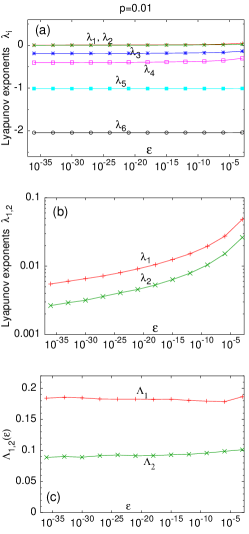
Figure 7: Characteristics of instability for Eqs (5,6,14) at $p$=0.01. (a),(b) conventional Lyapunov exponents; (c): length-related Lyapunov exponents

Indeed, at this level of graphical resolution we get an impression that at sufficiently small values of $\varepsilon$ the Lyapunov exponents tend to constant values, and their set with four negative and two vanishing values of $\lambda_{i}$ characterizes a motion along the attracting two-dimensional torus. However, a proper magnification of the region adjacent to zero (middle panel of Fig. 7) discloses that the saturation for the two largest exponents is deceptive: both exponents approach zero rather slowly, $\lambda_{1,2}(\varepsilon)\sim\ -1/\log\varepsilon$. At finite values of $\varepsilon$ the estimates $\lambda_{1,2}$ stay positive, indicating presence of two modes of instability, albeit rather weak.

Computation of conventional Lyapunov exponents $\lambda_{i}$ in accordance with (3) is ambiguous for the two largest ones. We are much better served if, instead, we use the length-related characteristics $\Lambda_{i}$, defined by Eq.(4). As visualized in Fig. 7(c), estimates of both length-related exponents $\Lambda_{1,2}$ stay nearly constant in the considered range of $\varepsilon$. This means that $\|\tilde{\mathbf{x}}_{1,2}(t)\|\sim\exp\big{(}\Lambda_{1,2}L(t)\big{)}$.

Similarly to the jargon based on conventional Lyapunov exponents where presence of two and more positive LE is called “hyperchaos”, here we can speak of “weak hyperchaos”. Of two positive exponents shown in Fig. 7c, the larger one stems from the $y$-subsystem of the equations (5,6) whereas the smaller one is related to the intrinsic dynamics of the $x$-subsystem.

Choosing the appropriate length

Before presenting reaction of $\Lambda_{1,2}$ to variation of the coupling amplitude $p$, an important technical aspect should be discussed. The flow (5,6) is a skew system: the variables $x_{i}$ act upon the set $\{y_{i}\}$ without reverse action. By construction, internal dynamics in the subspace $x_{i}$ ($i=1,2,3$) is independent of the value of $p$. Three of the six Lyapunov exponents characterize evolution of perturbations within this subspace and do not depend on $p$; in Fig. 7 these are, along with $\lambda_{2}$, the negative exponents $\lambda_{3}$ and $\lambda_{5}$. Being restricted to the internal dynamics of the subsystem $x$, the re-parameterized exponent $\Lambda_{2}$ should stay $p$-independent as well. However, the total length of the phase trajectory includes the coordinates $y_{i}$ and thereby depends on $p$; hence, it cannot be used in the evaluation of $\Lambda_{2}$, and should be replaced there by the length $L_{x}(t)$ of the projection onto the $x$-subspace. For a comparison of the growth rates of two instability modes, we cannot express them in terms of different lengths, hence below we substitute $L(t)$ in Eq.(4) by $L_{x}(t)$ both for $\Lambda_{1}$ and $\Lambda_{2}$.

Notably, for $\Lambda_{1}$ this procedure is not especially accurate at vanishing and very small values of $p$: as mentioned above, at $p=0$, $\Lambda_{1}$ characterizes the growth of instability in the isolated subsystem $y$ where a normalization with respect to $L_{y}$ would be an obvious choice. At very small $p$, the influence of the coupling subsystem $x$ is weak, and an evaluation in terms of $L_{x}$ may distort the whole picture. This is confirmed in the left panel of Fig. 8: there, the estimate of $\Lambda_{1}$ based on $L_{x}$ approaches the horizontal asymptote at small $\varepsilon$ distinctly slower than analogous estimates based on $L_{y}$ or the total length $L$. The length values have been determined in accordance with the following protocol: for all values of $\varepsilon$ (and further below, of the parameter $p$) the trajectory starts from the same initial conditions, and after a (discarded) transient of $10^{3}$ time units is further integrated for $5\times 10^{5}$ time units, producing a phase curve in the 6-dimensional phase space. For this curve, we calculate its total Euclidean length $L$ as well as the lengths of its projections onto the three-dimensional $x$- and $y$-subspaces: respectively, $L_{x}$ and $L_{y}$.

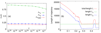
Figure 8: Characteristic lengths for phase trajectories of (5,6). Green, blue and red curves correspond to measurements based on, respectively, $L_{x}$, $L_{y}$ and the total length $L$. Integration interval: $t=5\times 10^{5}$. (a): Instability rate (4) at $p=0.01$ and variable $\bm{\varepsilon}$ in terms of different projections of trajectory. (b): Dependence of lengths on the coupling strength $p$ at $\varepsilon$=$10^{-27}$.

IV.3 Variation of the coupling strength

Variation of the parameter $p$ affects the dynamics of the system (5,6,14), both quantitatively and qualitatively. In the expression for the growth rate (4), this concerns $y$-related terms in the length $L$ of the reference orbit and in the norm $\|\tilde{\mathbf{x}}(t)\|$ of the perturbation. We start with the influence of $p$ upon $L$ under fixed observation time $t$. When, at constant $\varepsilon\neq 0$, the coupling $p$ is increased, repulsion near the saddles in the $y$-subspace weakens (quantitatively, this can be read off the respective saddle indices), hence the system stays longer in the neighborhoods of those saddles, and the average speed of motion across the $y$-subspace lowers. As a result, the total length of the reference orbit, as well as the length of its $y$-projection, decrease. This effect is illustrated in the right panel of Fig. 8. At low values of $p$, $y$-related components dominate in the total length; at larger $p$, in contrast, $L_{y}$ becomes much shorter than $p$-independent $L_{x}$, so that the difference between the total length and the length of $x$-projection becomes virtually negligible.

For estimates of the mean growth rates $\Lambda_{1,2}$ of perturbations we use the $p$-independent length $L_{x}(t)$, so that the entire effect is due to changes in the value of $\|\tilde{\mathbf{x}}(t)\|$. Recall that the rate $\Lambda_{2}$ characterizes the internal dynamics in the $x$-subsystem and is thereby insensitive to variations of $p$. In contrast, the value of $\Lambda_{1}$ (determined at $p$=0 by dynamics in the subspace $y$), varies when $p$ is changed. This is illustrated in Fig. 9.

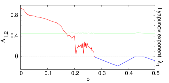
Figure 9: Red and green solid curves, respectively: length-related exponents $\Lambda_{1}$ and $\Lambda_{2}$. Blue solid curve: conventional (time-related) negative Lyapunov exponent. The value of $\varepsilon$ is fixed at $10^{-27}$.

As we see in the plot, increase of $p$ weakens this instability mode: the value of $\Lambda_{1}$ nearly monotonically decays until, at $p\approx$0.175 it becomes smaller than the exponent $\Lambda_{2}$. Further growth of $p$ results in a jagged non-monotonic pattern: probably, an indicator of internal transitions in this weakly chaotic state. Finally, $\Lambda_{1}$ changes sign close to $p=0.27$. There, this mode of slowly growing instability is replaced by the exponentially decaying perturbations, characterized by negative conventional Lyapunov exponent. Only one weakly chaotic component, corresponding to evolution of $x$-variables persists; in the projections of $y$-variables, there is almost no dynamics: practically all the time they hover close to the saddle points, and the total length of the trajectory $L$ nearly coincides with the length $L_{x}$ of the $x$-projection. In this way, the weakly chaotic dynamics close to the torus $T_{0}$ of the whole system is replaced by the “simpler” weakly chaotic dynamics near the heteroclinic contour of the master $x$-subsystem. Around $p\approx 0.45$ there is a short range of $p$ where the negative Lyapunov exponent nearly vanishes again; there, dynamics of the variables $y$ consists of short jerks, and the length of projection onto subspace $y$ becomes comparable with $x$-projection (cf. Fig. 8).

IV.4 Transformations in the phase space

Changes in the instability rates, imposed by variation of $p$, are reflected in changes of the phase portraits. In a reasonably broad parameter range $0\leq p\leq 0.27$, these changes appear to be mostly quantitative: the shape of phase trajectories is qualitatively persistent. Exemplary evolution of individual variables at two values of $p$ from this range is presented in Fig. 10. All variables display more or less ordered patterns. Recall that due to finite value of $\varepsilon$ the trajectories stay at a bounded distance from the invariant planes. For this reason, the times of residence in vicinities of the saddles, instead of forming the growing geometric progression (as would be the case at $\varepsilon=0$), weakly oscillate near the constant values. Remarkably, these values for two subsystems are different: there is no simple phase locking. In both subsystems we observe the typical winnerless competition. All three variables $x$ (top row) as well as all three $y$ variables (lower rows) oscillate in turn: while one of them traverses the high plateau, two other ones nearly vanish. For each variable in the $y$-system the plateaus consist of segments with three different heights: $y_{i}=\delta_{i}-\,p\sum_{j}\eta_{ij}x_{j}$ where $x_{j}$ are the coordinates of the master system at its saddle points. Differences between the plateau heights are proportional to $p$; they are weaker expressed in the left column of the plot, but are well visible (especially for the variable $y_{2}$) in the right column. At $p=0.22$ the temporal pattern is apparently weakly disordered; furthermore, the plateaus of $y_{2}$ are distinctly wider than the plateaus of other driven variables: epochs of activity of $y_{3}$ and, especially, of $y_{1}$ turn into the sharp spikes separated by uneven intervals.

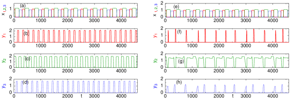
Figure 10: Dynamics on the non-smooth torus: Temporal evolution of the system (5,6,14) at $\varepsilon=10^{-18}$. Left column: $p$=0.05; right column: $p$=0.22. Top row: variables of the master system. Lower rows: variables of the forced $y$ system.

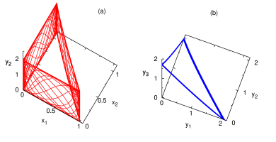
Figure 11: Projections of the phase portrait of the system (5,6,14) at $p=0.05$, $\varepsilon=10^{-18}$.

Characteristic projections of the phase portrait onto three-dimensional subspaces for this oscillatory state are shown in Fig. 11. In the master $x$-subsystem (not shown) we observe just the attracting heteroclinic contour. A plot with two coordinates from the master system and one coordinate from the driven $y$-subsystem (left panel of Fig. 11) has the shape of a right triangular prism; equilibria are projected onto vertices whereas the unstable manifolds run along the edges. At finite $\varepsilon$ the attracting orbits escape the vertices along the faces of the prism.

The projection with coordinates entirely from the driven subsystem (right panel of Fig. 11) has a triangular shape. Recall that each vertex of the triangle results from projecting of three different (and well separated in terms of coordinates $x_{i}$) points of equilibrium from the $x$-system. In terms of the coordinates $y_{i}$, the distances between these three projections are proportional to $p$, and a closer look in Fig. 12 shows that the triangle possesses a “width”: its vertices (and, correspondingly the whole phase portrait) split into three components. Deceptively close on the $y$-projection, these components are macroscopically separated in terms of the $x$-coordinates.

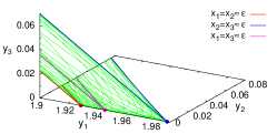
Figure 12: Blowup of the phase space region near the $y_{2}$-axis. Filled circles and thicker curves: points of equilibrium and their separatrices. Parameter values like in Fig. 11.

.

At still higher values of $p$ the picture changes drastically: in the range $0.28\leq p\leq 0.42$ only the variable $y_{2}$ survives in the driven system whereas the variables $y_{1}$ and $y_{3}$ completely decay (numerically both of them attain the value of $\varepsilon$). An example of evolution of $y_{2}$ is presented in Fig. 13a: it consists of horizontal plateaus connected by segments of rapid transitions. Comparison with dynamics of variables of the master system in the panel 13b shows that each plateau corresponds to the epoch of activity for one of the master variables. At 0.43$\leq p\leq$ 0.45 a further regime is observed (Fig. 13c,d) in which only $y_{3}$ decays whereas $y_{1}$ and $y_{2}$ alternate in activity. Finally, beyond $p=0.45$ the driven system returns to the state with only one active variable that jumps between three plateaus (Fig. 13e,f); this time it is the variable $y_{1}$ whereas $y_{2}$ and $y_{3}$ decay. The reasons for this profound change in dynamics can be understood from the plot of parameter dependence of the overall saddle indices of the heteroclinic contours (see Sect.III): the products of saddle indices over all saddles participating in the contour Afr_MIR_Varona_2004 .

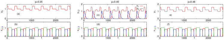
Figure 13: Dynamics after the breakup of the non-smooth torus: Temporal evolution of the system (5,6,14) at $\varepsilon=10^{-18}$. Left column: $p$=0.35; middle column: $p$=0.45; right column: $p$=0.48. Top row: non-decaying variables of the driven system: (a) $y_{2}$; (c) $y_{1,2}$; (e) $y_{1}$. Bottom row: variables of the master system: $x_{1},x_{2},x_{3}$.

The non-smooth torus at small $|p|$ is built from several heteroclinic contours: when the master $x$ is frozen at one of its saddle equilibria, the driven system has three saddle points whose one-dimensional unstable manifolds form a contour. Altogether there are three such contours, and for each of them the overall saddle index should be checked separately, taking into account only the eigenvalues pertaining to the $y$-subspace. Recall: a heteroclinic contour is attracting if its overall index exceeds 1.

Fig. 14 shows dependence of all three overall indices on the coupling strength $p$. For each curve, an initial weak decrease is superseded by subsequent growth: attraction to the contours becomes stronger. Remarkably, the saddle indices of separate saddles may decrease and fall below 1 (not shown in Fig. 14); what matters, however, are not the separate indices but their overall product – and it grows! Furthermore, one by one, the values of the overall products diverge: one of the respective positive eigenvalues becomes small and finally vanishes: the equilibrium loses instability and turns from the saddle into the stable node.

Figure 14: Overall saddle indices, composed of eigenvalues, leading in the $y$-subspace. Coloring denotes location of the saddle point in the $x$-subspace: $(x_{1}$=$\sigma_{1},\,x_{2}$=$x_{3}$=0) for the red curve, $(x_{1}$=0, $x_{2}$=$\sigma_{2},\,x_{3}$=0) for the green curve, and $(x_{1}$=$x_{2}$=0, $x_{3}$=$\sigma_{3})$ for the blue curve. Dotted vertical lines: stabilization (via transcritical bifurcations) of respective saddles. Note: growth of overall indices does not exclude the decrease of indices of separate saddles (not shown here).

For an equilibrium lying on the coordinate axis of the $y$-subsystem, stabilization is a result of the transcritical bifurcation. With the master system frozen at one of its saddles, the driven subsystem, along with a set of three such “axial” equilibria, possesses three further steady states, one in each of the invariant planes $y_{i}$=0, $i=1,2,3$. At $p$=0 all three “in-plane” states have, beside zero, a positive and a negative coordinate $y_{i}$; thereby, they lie in the “non-physical” part of the phase space. Two of these states are asymptotically stable in the subspace $y$ whereas the third one is a saddle with one negative and two positive Jacobian eigenvalues. Since the coordinates of these equilibria are linear functions of the coupling $p$, some of them move into the positive octant when $p$ is increased. Crossing on their way the pertaining coordinate axis, they collide with the corresponding “axial” equilibrium. In the course of this transcritical bifurcation, the equilibria exchange stability, and the axial one becomes stable. Explicit expressions for the bifurcation parameter values are too lengthy to be quoted here.

Stabilization of the former saddle(s) changes the dynamics of $y$ at frozen $x$: now there is a simple attractor, the subsystem eventually converges to it and stays there forever. “Unfreezing” $x$ leads to rapid switches in the dynamics of the driven subsystem: arrival of the master system at its next saddle point implies for the driven one a new structure of the phase space, where there may still be three saddle points and a heteroclinic contour, or, instead, a steady “axial” attractor at which the driven system resides until the next switch. In the latter case two of the coordinates $y_{i}$ decay whereas the third one assumes the equilibrium value. In the course of the further increase of $p$, stabilization of saddle states, step by step, occurs in all three “frozen” subspaces, and finally heteroclinic dynamics in the driven system dies out. In the situations of the left and right columns of Fig.13, the stable equilibria before/after the switch lie on the same coordinate axis, hence the evolution of the driven subsystem becomes effectively one-dimensional; in the middle column, the driven subsystem jumps between equilibria on two axes, keeping the third coordinate negligible.

The states in the left and right columns of Fig.13 illustrate replacement of the winnerless competition in the slave subsystem $y$ by the quasi-steady “winner-take-all” situation: As long as the master $x$ remains in the nearly static configuration at one of its saddle-points, the slave subsystem synchronizes with it, becoming static as well. Nontrivial dynamics emerges in the situation of “nimble master, lazy slave” when the typical time of heteroclinic switching in the master subsystem is smaller than the time of relaxation to the equilibrium in the slave subsystem; details of this dynamics will be reported elsewhere.

Alteration of quasi-steady states also explains the practically piecewise-linear dependence on $p$ of the negative Lyapunov exponent (blue solid curve in Fig. 9 above). In those states, the driven subsystem jumps between the (emerging) stable equilibria, and the Lyapunov exponent is just the weighted sum of the least negative Jacobian eigenvalues of these equilibria; the weights are the normalized lengths of the corresponding plateaus. Since all eigenvalues are linear functions of $p$, their weighted sum is it as well.

V Discussion

In this paper, we have discussed coordination among coupled heteroclinic networks, whose dynamics mimics sequential switching of metastable information units. Coupled networks of this kind exist on different levels of brain elements hierarchy. The hierarchy itself results from complex functional interactions, residing between the poles of segregation and integration tendencies for networks that perform joint specific cognitive and/or behavioral tasks. In particular, we have suggested the dynamical mechanism of low-dimensional coordination that is related to the general information processing in the brain sequential units Baldassano_et_al_2017 . The key phenomenon of this coordination is entrainment of localized units in multimodal brain activity RAV_2010 .

For the upper level of network hierarchy we have proposed a low-dimensional mathematical model of the brain-to brain interaction. The model belongs to the class of generalized Lotka-Volterra systems that, when decoupled, feature rhythmic activity. Regimes, observed in the phase space in the case of the simplest master-slave configuration, can be viewed as mathematical images of the corresponding cognitive processes. Under sufficiently weak coupling, the attractor is a non-smooth two-dimensional torus that contains equilibrium points of the saddle type and is composed of heteroclinic orbits joining those points. Instability of all trajectories in the basin of the attractor is confirmed by presence of two positive length-related Lyapunov exponents. Typical pattern of behavior on the attractor is successive switching between the saddles along different heteroclinic channels AGR . Under stronger coupling the system undergoes a bifurcation related to the breakup of the invariant torus. After the breakup, the winnerless competition dynamics in the slave subsystem is replaced by the winner-take-all quasistatics. This restricts the number of options in the slave subsystem and makes cooperation between the master and the slave more rigid.

Proper account of fluctuations.  In numerical studies we have substituted the fluctuating terms in the equations (e.g., explicit multiplicative noise) by the formal construction that keeps trajectories from coming too close to the invariant hyperplanes. Replacement is justified by the fact that the sole role of fluctuations, regardless of their explicit shape, is to kick the system out of the vicinities of the equilibria where, otherwise, the system would spend the overwhelming proportion of its time. Therefore, we expect qualitatively the same results if, instead, the stochastic version of Eq.(II) is simulated.

A few words about bidirectional coupling.  Our analysis has been restricted to unilateral coupling; in the dynamical system (II) this corresponds to vanishing parameter $q$, responsible for the reverse influence of the participant $Y$ upon the participant $X$. Part of our results can be extended to the case of bidirectional interaction; this refers, in particular, to the existence at weak coupling rates of the attracting non-smooth torus with the heteroclinic network. The proof in Sect. III is based on presence of the torus in the case of decoupled subsystems and on the continuity arguments for sufficiently weak unilateral coupling $p$. Similar continuity arguments ensure persistence of this attractor under sufficiently small values of reverse coupling $q$ as well. Accordingly, the system with weak two-way coupling should also feature the “toroidal” winnerless competition, with heteroclinic channels between the saddles formed not along one-dimensional separatrices but along two-dimensional manifolds. Substantial increase of either (or both) of the coupling coefficients $p$ and $q$ enforces the breakup of the non-smooth torus; along with the mechanism described above (partial regain of stability by the saddle points in one of the subsystems), other scenarios can develop as well, e.g., loss of attraction by some of the heteroclinic contours and subsequent “smoothing” of respective corners of the attractor. Details of these effects will be reported elsewhere.

Master-slave case: are we slaves of our memories? As mentioned in the Introduction, unidirectional configuration of coupling can model the influence of episodic memory in the past upon memory dynamics in the future. In this respect, the winner-takes-all behavior described in the end of the preceding section might be of interest for certain kinds of mental disorder where attention of a patient is rigidly fixed at a few past events: the past memory (master) cyclically switches between several episodes with long stay at each of them; during these stays, the current memory (driven subsystem) stays frozen, but as soon as the past episode changes, the equilibrium of the current memory ceases to exist, and the memory abruptly moves on to its new tentative attractor.

Brain-to-Brain information generation. Episodic memory for real life involves the orchestration of multiple time scales dynamical processes, including hierarchical chunking and multimodal binding of events. To concentrate at the core of the phenomenon of episodic entrainment, we have restricted our treatment to the simplest approximation. We supposed that the characteristic time of episodes forming i.e., chunking $t_{\rm ch}$ is much shorter than the characteristic time $t_{\rm ep}$ of sequential switching between episodes. Based on the generalized hierarchical model of episodic memory Varona_Rabinovich_2016 , entrainment with arbitrary ratio $t_{\rm ch}\ll t_{\rm ep}$ can be considered. Interesting new dynamics is expected within this modeling framework. In particular, confusion or entanglement of the events from different episodes in the entrainment memory can occur. The dynamical origin of such memory errors can be the overlap of weakly chaotic time series representing different episodes in the sequential entrainment process (about the neurophysiological origin of the errors and distortion in the episodic memory see, for example, Schacter_2012 ). To estimate the level of information generated in the error sequence of episodes, the technics suggested in Rabinovich_etal_2012 can be employed.

References

- (1) A. Zadbood, J. Chen, Y. C. Leong, K. A. Norman, U. Hasson, How We Transmit Memories to Other Brains: Constructing Shared Neural Representations Via Communication, Cerebral Cortex 27, 4988 (2017).
- (2) L. M. Bietti, Sharing memories, family conversation and interaction, Discourse & Society 21, 499 (2010).
- (3) A. C. Heusser, Y. Ezzyat, I. Shiff, L. Davachi, Perceptual Boundaries Cause Mnemonic Trade-Offs Between Local Boundary Processing and Across-Trial Associative Binding. (2017) https://psyarxiv.com/z3tsd/ .
- (4) T. Sadeh, D. Shohamy, D. R. Levy, N. Reggev, A. Maril, Cooperation between the Hippocampus and the Striatum during Episodic Encoding, J. of Cognitive Neuroscience 23, 1597 (2011).
- (5) S. H. P. Collin, B. Milivojevic, C. F. Doelle, Hippocampal hierarchical networks for space, time, and memory, Current Opinion in Behavioral Sciences 17, 71 (2017).
- (6) Z. Ma, N. Zhang, Temporal transitions of spontaneous brain activity, Elife. 7, e33562 (2018). DOI: https://doi.org/10.7554/eLife.33562
- (7) A. E. Hudson, D. P. Calderon, D. W. Pfaff, A. Proekt, Recovery of consciousness is mediated by a network of discrete metastable activity states PNAS 111, 9283 (2014).
- (8) J. M. Shine, M. Breakspear, P. Bell, K. E. Martens, R. Shine, O. Koyejo, O. Sporns, R. Poldrack, The low dimensional dynamic and integrative core of cognition in the human brain, bioRxiv 266635 (2017); doi: https://doi.org/10.1101/266635.
- (9) A. Slaps̆inskaite, R. Hristovski, S. Razon, N. Balagué, G. Tenenbaum, Metastable Pain-Attention Dynamics during Incremental Exhaustive Exercise, Frontiers in Psychology 7, 2054 (2017).
- (10) C. Baldassano, J. Chen, A. Zadbood, J. W. Pillow, U. Hasson, K. A. Norman, Discovering Event Structure in Continuous Narrative Perception and Memory, Neuron 95, 709 (2017).
- (11) K. J. Friston, The labile brain. I. Neuronal transients and nonlinear coupling, Phil.Trans. R. Soc. Lond. B 355, 215 (2000) 215.
- (12) E. Tognoli, J. A. S. Kelso, The Metastable Brain, Neuron 81, 36 (2014).
- (13) L. Cocchi, L. L. Gollo, A. Zalesky, M. Breakspear, Criticality in the brain: A synthesis of neurobiology, models and cognition, Progress in Neurobiology 158, 132 (2017).
- (14) J. Chen, Y. C. Leong, C. J. Honey, C. H. Yong, K. A. Norman, U. Hasson, Shared memories reveal shared structure in neural activity across individuals, Nature Neuroscience 20, 115 (2017).
- (15) C. Baldassano, D. M. Beck, L. Fei-Fei, Human-object interactions are more than the sum of their parts, Cerebral Cortex 27, 2276 (2017).
- (16) D. J. Beal, H. M. Weiss, The episodic structure of life at work, Chapter 2 in: A Day in the Life of a Happy Worker, Eds: A. B. Bakker and K. Daniels, Psychology Press, London (2013).
- (17) M. I. Rabinovich, P. Varona, I. Tristan, V. S. Afraimovich, Chunking Dynamics: Heteroclinics in Mind, Front. Comput. Neurosci. 8, 22 (2014).
- (18) B. I. Cohn-Sheehy, C. Ranganath, Time regained: how the human brain constructs memory for time, Current Opinion in Behavioral Sciences 17, 169 (2017).
- (19) D. Clewett, L. Davachi, The ebb and flow of experience determines the temporal structure of memory, Current Opinion in Behavioral Sciences 17, 186 (2017).
- (20) M. I. Rabinovich, R. Huerta, P. Varona, V. S. Afraimovich, Transient cognitive dynamics, metastability, and decision making, PLoS Comput. Biol. 4, e1000072 (2008).
- (21) M. I. Rabinovich, A. N. Simmons, P. Varona, Dynamical bridge between brain and mind, Trends in Cognitive Sciences 19, 453 (2015).
- (22) C. Bick, M. I. Rabinovich, Dynamical origin of the effective storage capacity in the brain’s working memory, Phys. Rev. Lett. 103, 218101 (2009).
- (23) D. H. Ingvar, “Memory of the future”: an essay on the temporal organization of conscious awareness, Hum. Neurobiol. 4, 127 (1985).
- (24) K. K. Szpunar, D. R. Addis, V.C. McLelland, D. L. Schacter, Memories of the future: new insights into the adaptive value of episodic memory, Front. Behavioral Neurosci. 7, 47 (2013).
- (25) D. L. Schacter, D. R. Addis, K. K. Szpunar, Escaping the Past: Contributions of the Hippocampus to Future Thinking and Imagination, In: The Hippocampus from Cells to Systems, D. E. Hannula, M. C. Duff (eds.), Springer, p.439 (2017).
- (26) P. Varona, M. I. Rabinovich, Hierarchical dynamics of informational patterns and decision-making, Proc. Royal Soc. B 283, 20160475 (2016).
- (27) C. J. Gómez-Ariza, F. del Prete, L. Prieto del Val, T. Valle, M. T. Bajo, A Fernandez, Memory inhibition as a critical factor preventing creative problem solving. J. of Experimental Psychology: Learning, Memory, and Cognition 43, 986 (2017).
- (28) M. I. Rabinovich, R. Huerta, and P. Varona, Heteroclinic synchronization: ultrasubharmonic locking. Phys. Rev. Lett. 96, 141001 (2006).
- (29) C. Grebogi, E. Ott, J. A. Yorke, Crises, sudden changes in chaotic attractors and transient chaos, Physica D 7, 181 (1983).
- (30) V. S. Afraimovich, A. B. Neiman, Weak Transient Chaos. In: Advances in Dynamics, Patterns, Cognition (Eds: I. S. Aranson, A. Pikovsky, N. F. Rulkov, L. S. Tsimring) Nonlinear Systems and Complexity 20, Springer, p. 3 (2017).
- (31) V. Afraimovich, D. Cuevas, T. Young, Sequential dynamics of a master-slave system, Dyn. Syst. 28, 154 (2013).
- (32) M. Agurval, A. Rodrigues, M. Field, Dynamics near the product of planar heteroclinic attractors, Dyn. Syst. 4, 199 (2011).
- (33) V. Afraimovich, G. Moses, T. Young, Two-dimensional heteroclinic attractor in the generalized Lotka-Volterra System, Nonlinearity 29, 1645 (2016).
- (34) L. P. Shilnikov, A. L. Shilnikov, D. V. Turaev, L. O. Chua, Methods of Qualitative Theory in Nonlinear Dynamics. World Scientific (1998), New Jersey.
- (35) V. S. Afraimovich, V. P. Zhigulin, M. I. Rabinovich, On the origin of reproducible sequential activity in neural circuits, Chaos 14, 1123 (2004).
- (36) M. I. Rabinovich, V. S. Afraimovich, P. Varona, Heteroclinic Binding, Dynamical Systems 25, 433 (2010).
- (37) V. Afraimovich, X. Gong, M. Rabinovich, Sequential memory: Binding dynamics, Chaos 25, 103118 (2015).
- (38) V. Afraimovich, S. B. Hsu, Lectures in Chaotic Dynamics, AMS/IP Studies in Advanced Mathematics 28, International Press, 2003.
- (39) V. S. Afraimovich, M. I. Rabinovich, P. Varona, Heteroclinic contours in neural ensembles and the winnerless competition principle, Int. J. Bifurcation Chaos 14, 1195 (2004).
- (40) D. L. Schacter, Constructive memory: past and future, Dialogues Clin. Neurosci. 14, 7 (2012).
- (41) M. I. Rabinovich, V. S. Afraimovich, C. Bick, and P. Varona, Information flow dynamics in the brain, Phys. Life Rev. 9, 51 (2012).