Join Query Optimization Techniques for Complex Event Processing Applications

Abstract

Complex event processing (CEP) is a prominent technology used in many modern applications for monitoring and tracking events of interest in massive data streams. CEP engines inspect real-time information flows and attempt to detect combinations of occurrences matching predefined patterns. This is done by combining basic data items, also called “primitive events”, according to a pattern detection plan, in a manner similar to the execution of multi-join queries in traditional data management systems. Despite this similarity, little work has been done on utilizing existing join optimization methods to improve the performance of CEP-based systems.

In this paper, we provide the first theoretical and experimental study of the relationship between these two research areas. We formally prove that the CEP Plan Generation problem is equivalent to the Join Query Plan Generation problem for a restricted class of patterns and can be reduced to it for a considerably wider range of classes. This result implies the NP-completeness of the CEP Plan Generation problem. We further show how join query optimization techniques developed over the last decades can be adapted and utilized to provide practically efficient solutions for complex event detection. Our experiments demonstrate the superiority of these techniques over existing strategies for CEP optimization in terms of throughput, latency, and memory consumption.

1 Introduction

Complex event processing has become increasingly important for applications in which arbitrarily complex patterns must be efficiently detected over high-speed streams of events. Online finance, security monitoring, and fraud detection are among the many examples. Pattern detection generally consists of collecting primitive events and combining them into potential (partial) matches using some type of detection model. As more events are added to a partial match, a full pattern match is eventually formed and reported. Popular CEP mechanisms include nondeterministic finite automata (NFAs) [5, 18, 50], finite state machines [6, 44], trees [35], and event processing networks [21, 41].

A CEP engine creates an internal representation for each pattern $P$ to be monitored. This representation is based on a model used for detection (e.g., an automaton or a tree) and reflects the structure of $P$. In some systems [5, 50], the translation from a pattern specification to a corresponding representation is a one-to-one mapping. Other frameworks [6, 29, 35, 41, 44] introduce the notion of a cost-based evaluation plan, where multiple representations of $P$ are possible, and one is chosen according to the user’s preference or some predefined cost metric.

We will illustrate the above using the following example. Assume that we are receiving periodical readings from four traffic cameras A, B, C and D. We are required to recognize a sequence of appearances of a particular vehicle on all four cameras in order of their position on a road, e.g., $A\rightarrow B\rightarrow C\rightarrow D$. Assume also that, due to a malfunction in camera D, it only transmits one frame for each 10 frames sent by the other cameras.

Figure 1LABEL:sub@fig:nfa-no-reordering displays a nondeterministic finite automaton (NFA) for detecting this pattern, as described in [50]. A state is defined for each prefix of a valid match. During evaluation, a combination of camera readings matching each prefix will be represented by a unique instance of the NFA in the corresponding state. Transitions between states are triggered nondeterministically by the arrival of an event satisfying the constraints defined by the pattern. A new NFA instance is created upon each transition.

The structure of the above automaton is uniquely dictated by the order of events in the given sequence. However, due to the low transmission rate of D, it would be beneficial to wait for its signal before examining the local history for previous readings of A, B and C that match the constraints. This way, fewer prefixes would be created. Figure 1LABEL:sub@fig:nfa-with-reordering demonstrates an out-of-order NFA for the rewritten pattern (defined as “Lazy NFA” in [29]). It starts by monitoring the rarest event type D and storing the other events in the dedicated buffer. As a reading from camera D arrives, the buffer is inspected for events from A, B and C preceding the one received from D and located in the same time window. This plan is more efficient than the one implicitly used by the first automaton in terms of the total number of partial matches created during evaluation. Moreover, unless more constraints on the events are defined, it is the cheapest among all $\left(4!\right)$ available plans, that is, all mutual orders of A, B, C and D.

Not all CEP mechanisms represent a plan as an evaluation order. In Figure 1LABEL:sub@fig:zstream-abcd a tree-based evaluation mechanism [35] for detecting the above pattern is depicted. Events are accepted at the corresponding leaves of the tree, and passed towards the root where full matches are reported. Note that this model requires an evaluation plan to be supplied, because, for a pattern of size $n$, there are at least $C_{n-1}=\frac{\left(2n-2\right)!}{\left(n-1\right)!n!}$ possible trees (where $C_{n}$ is the $n^{th}$ Catalan number).

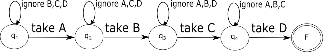
(a)

(b)

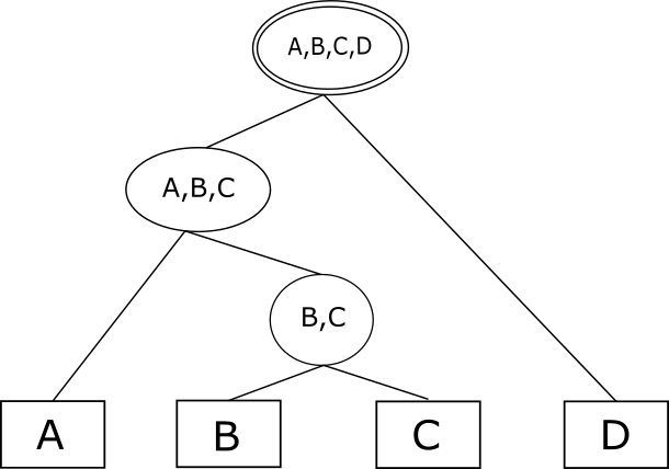
(c)

Figure 1: Evaluation structures for a CEP pattern SEQ(A,B,C,D): LABEL:sub@fig:nfa-no-reordering NFA with no reordering; LABEL:sub@fig:nfa-with-reordering NFA with reordering; LABEL:sub@fig:zstream-abcd evaluation tree.

In many scenarios, we will prefer the evaluation mechanisms supporting cost-based plan generation over those mechanisms allowing for only one such plan to be defined. This way, we can drastically boost system performance subject to selected metrics by picking more efficient plans. However, as the space of potential plans is at least exponential in pattern size, finding an optimal evaluation plan is not a trivial task.

Numerous authors have identified and targeted this issue. Some of the proposed solutions are based on rewriting the original pattern according to a set of predefined rules to maximize the efficiency of its detection [41, 44]. Other approaches discuss various strategies and algorithms for generating an evaluation plan that maximizes the performance for a given pattern according to some cost function [6, 29, 35]. While the above approaches demonstrate promising results, this research field remains largely unexplored, and the space of the potential optimization techniques is still far from being exhausted.

The problem described above closely resembles the problem of estimating execution plans for large join queries. As opposed to CEP plan generation, this is a well-known, established, and extensively targeted research topic. A plethora of methods and approaches producing close-to-optimal results were published during the last few decades. These methods range from simple greedy heuristics, to exhaustive dynamic programming techniques, to randomized and genetic algorithms [31, 32, 36, 45, 46, 47]. Figure 2 illustrates two main types of execution plans for join queries, a left-deep tree (2LABEL:sub@fig:left-deep-tree) and a bushy tree (2LABEL:sub@fig:bushy-tree) [25].

(a)

(b)

Figure 2: Execution plans for a join of four relations $R_{1},R_{2},R_{3},R_{4}$: LABEL:sub@fig:left-deep-tree a left-deep tree; LABEL:sub@fig:bushy-tree a bushy tree.

Both problems look for a way to efficiently combine multiple data items such that some cost function is minimized. Also, both produce solutions possessing similar structures. If we reexamine Figures 1 and 2, we can see that left-deep tree plans (2LABEL:sub@fig:left-deep-tree) and bushy tree plans (2LABEL:sub@fig:bushy-tree) closely resemble evaluation plans for NFAs (1LABEL:sub@fig:nfa-with-reordering) and trees (1LABEL:sub@fig:zstream-abcd) respectively. An interesting question is whether join-related techniques can be used to create better CEP plans using a proper reduction.

In this work, we attempt to close the gap between the two areas of research. We study the relationship between CEP Plan Generation (CPG) and Join Query Plan Generation (JQPG) problems and show that any instance of CPG can be transformed into an instance of JQPG. Consequently, any existing method for JQPG can be made applicable to CPG. Our contributions can be summarized as follows:

• We formally prove the equivalence of JQPG and CPG for a large subset of CEP patterns, the conjunctive patterns. The proof addresses the two major classes of evaluation plans, the order-based plans and the tree-based plans (Section 4).

• We extend the above result by showing how other pattern types can be converted to conjunctive patterns, thus proving that any instance of CPG can be reduced to an instance of JQPG (Section 5).

• The deployment of a JQPG method to CPG is not trivial, as multiple CEP-specific issues need to be addressed, such as detection latency constraints, event consumption policies, and adaptivity considerations. We present and discuss the steps essential for successful adaptation of JQPG techniques to the CEP domain (Section 6).

• We validate our theoretical analysis in an extensive experimental study. Several well-known JQPG methods, such as Iterative Improvement [47] and Dynamic Programming [45], were applied on a real-world event dataset and compared to the existing state-of-the-art CPG mechanisms. The results demonstrate the superiority of the adapted JQPG techniques (Section 7).

2 Complex Event Processing

In this section, we introduce the notations used throughout this paper and provide the necessary background on complex event processing. We present the elements of a CEP pattern, including a brief taxonomy of commonly used pattern types. Then, we describe two classes of CEP evaluation mechanisms that are the focus of this work: the order-based and the tree-based CEP. The results obtained in the later sections are based on but not limited to these two representation models, and they can be extended to more complex schemes, such as event processing networks [21, 41].

2.1 CEP Patterns

The patterns recognized by CEP systems are normally formed using declarative specification languages [14, 18, 50]. A pattern is defined by a combination of primitive events, operators, a set of predicates to be satisfied by the participating events, and a time window. Each event is represented by a type and a set of attributes, including the occurrence timestamp. The operators describe the relations between different events comprising a pattern match. The predicates, usually organized in a Boolean formula, specify the constraints on the attribute values of the events. As an example, consider the following pattern specification syntax, taken from SASE [50]:

$$\begin{array}[]{l}PATTERN\>op\left(T_{1}\>e_{1},T_{2}\>e_{2},\cdots,T_{n}\>e_{n}\right)\\ WHERE\>(c_{1,1}\wedge c_{1,2}\wedge\cdots\wedge c_{n,n-1}\wedge c_{n,n})\\ WITHIN\>W.\end{array}$$

Here, the PATTERN clause specifies the events $e_{1},\cdots,e_{n}$ we would like to detect and the operator $op$ to combine them (see below). The WHERE clause defines a Boolean CNF formula of inter-event constraints, where $c_{i,j};1\leq i,j\leq n$ stands for the mutual condition between attributes of $e_{i}$ and $e_{j}$. $c_{i,i}$ declares filter conditions on $e_{i}$. Any of $c_{i,j}$ can be empty. For the rest of our paper, we assume that all conditions between events are at most pairwise (i.e., a single condition involves at most two different events). This assumption is for presentational purposes only, as our results can be easily generalized to arbitrary predicates. The WITHIN clause sets the time window $W$, which is the maximal allowed difference between the timestamps of any pair of events in a match.

Throughout this work we assume that each primitive event has a well-defined type, i.e., the event either contains the type as an attribute or it can be easily inferred from other attributes using negligible system resources. While this constraint may seem limiting, it is easy to overcome in most cases by redefining what a pattern creator considers a type.

In this paper, we will consider the most commonly used operators, namely AND, SEQ, and OR. The AND operator requires the occurrence of all events specified in the pattern within the time window. The SEQ operator extends this definition by also expecting the events to appear in a predefined temporal order. The OR operator corresponds to the appearance of any event out of those specified.

Two additional operators of particular importance are the negation operator (NOT) and the Kleene closure operator (KL). They can only be applied on a single event and are used in combination with other operators. $NOT\left(e_{i}\right)$ requires the absence of the event $e_{i}$ from the stream (or from a specific position in the pattern in the case of the SEQ operator), whereas $KL\left(e_{i}\right)$ accepts one or more instances of $e_{i}$. In the remainder of this paper, we will refer to NOT and KL as unary operators, while AND, SEQ and OR will be called n-ary operators.

The PATTERN clause may include an unlimited number of n-ary and unary operators. We will refer to patterns containing a single n-ary operator, and at most a single unary operator per primitive event, as simple patterns. On the contrary, nested patterns are allowed to contain multiple n-ary operators (e.g., a disjunction of conjunctions and/or sequences will be considered a nested pattern). Nested patterns present an additional level of complexity and require advanced techniques (e.g., as described in [33]).

We will further divide simple patterns into subclasses. A simple pattern whose n-ary operator is an AND operator will be denoted as a conjunctive pattern. Similarly, sequence pattern and disjunctive pattern will stand for patterns with SEQ and OR operators, respectively. In addition, a simple pattern containing no unary operators will be called a pure pattern.

The “four cameras pattern” described in Section 1 illustrates the above. This is a pure sequence pattern, written in SASE as follows:

$$\begin{array}[]{l}PATTERN\>SEQ\left(A\>a,B\>b,C\>c,D\>d\right)\\ WHERE\>(a.vehicleID=b.vehicleID=\\ \qquad\qquad=c.vehicleID=d.vehicleID)\\ WITHIN\>W.\end{array}$$

The following example depicts a nested pattern, consisting of a (non-pure) conjunctive pattern and an inner pure disjunctive pattern:

$$\begin{array}[]{l}PATTERN\>AND\left(A\>a,NOT\left(B\>b\right),OR\left(C\>c,D\>d\right)\right)\\ WITHIN\>W.\end{array}$$

2.2 Order-based Evaluation Mechanisms

Order-based evaluation mechanisms play an important role in CEP engines based on state machines. One of the most commonly used models following this principle is the NFA (nondeterministic finite automaton) [5, 18, 50]. An NFA consists of a set of states and conditional transitions between them. Each state corresponds to a prefix of a full pattern match. Transitions are triggered by the arrival of the primitive events, which are then added to partial matches. Figures 1LABEL:sub@fig:nfa-no-reordering and 1LABEL:sub@fig:nfa-with-reordering depict an example of two NFAs constructed for the same sequence pattern using different order-based plans. While in theory NFAs may possess an arbitrary topology, non-nested patterns are normally detected by a chain-like structure.

The basic NFA model does not include any notion of altering the “natural” evaluation order or any other optimization based on pattern rewriting. Multiple works have presented methods for constructing NFAs with out-of-order processing support. W.l.o.g., we will use the Lazy NFA mechanism, a chain-structured NFA introduced in [28, 29] and capable of following a specified evaluation order.

Given a pattern of $n$ events and a user-specified order $O$ on the event types appearing in the pattern, a chain of $n+1$ states is constructed, with each state $k$ corresponding to a match prefix of size $k-1$. The order of the states matches $O$ (i.e., the transition from the initial state to the second one expects the first type in $O$, the transition from the second to the third state expects the second type in $O$, etc.). The $\left(n+1\right)^{th}$ state in the chain is the accepting state. To achieve out-of-order evaluation, NFA instances store events which arrive out-of-order. A buffered event is retrieved and processed when its corresponding state in the chain is reached. During a traversal attempt on an edge connecting two adjacent states $q_{i}$ and $q_{i+1}$, the following conditions will be verified: $\left\{c_{i+1,j}|e_{j}\>precedes\>e_{i+1}\>in\>O\right\}$.

This construction method allows us to apply all possible $\left(n!\right)$ orders. Note that the detection correctness is not affected, i.e., all $\left(n!\right)$ NFAs will track the exact same pattern.

2.3 Tree-based Evaluation Mechanisms

An alternative to NFA, the tree-based evaluation mechanism [35] specifies which subsets of full pattern matches are to be tracked by defining tree-like structures. For each event participating in a pattern, a designated leaf is created. During evaluation, events are routed to their corresponding leaves and are buffered there. The non-leaf nodes accumulate the partial matches. The computation at each non-leaf node proceeds only when all of its children are available (i.e., all events have arrived or partial matches have been calculated). Matches formed at the tree root are reported to the end users. An example is shown in Figure 1LABEL:sub@fig:zstream-abcd.

The main advantage of the tree-based evaluation mechanism over NFA is its flexibility. Instead of relying on a single evaluation order, it allows primitive events to arrive in any possible order and still be efficiently processed.

ZStream assumed a batch-iterator setting [35]. To perform our study under a unified framework, we modify this behavior to support arbitrary time windows. As described above with regard to NFAs, a separate tree instance will be created for each currently found partial match. As a new event arrives, an instance will be created containing this event. Every instance $I$ corresponds to some subtree $s$ of the tree plan, with the leaves of $s$ holding the primitive events in $I$. Whenever a new instance $I^{\prime}$ is created, the system will attempt to combine it with previously created “siblings”, that is, instances corresponding to the subtree sharing the parent node with $s^{\prime}$. As a result, another new instance containing the unified subtree will be generated. This in turn will trigger the same process again, and it will proceed recursively until the root of the tree is reached or no siblings are found.

Contrary to the basic version of NFA [5, 18, 50], ZStream includes an algorithm for determining the optimal tree structure for a given pattern. This algorithm is based on a cost model that takes into account the arrival rates of the primitive events and the selectivities of their predicates. However, since leaf reordering is not supported, a subset of potential plans is missed. We will illustrate this drawback using the following example:

$$\begin{array}[]{l}PATTERN\>SEQ\left(A\>a,B\>b,C\>c\right)\\ WHERE\>(a.x=c.x)\\ WITHIN\>W.\end{array}$$

We assume that all events arrive at identical rates, and that the condition between A and C is very restrictive. Figures 3LABEL:sub@fig:zstream-abc-left and 3LABEL:sub@fig:zstream-abc-right present the only two possible plans according to the algorithm presented in [35]. However, due to the condition between A and C, the most efficient evaluation plan is the one displayed in Figure 3LABEL:sub@fig:zstream-abc-reordering. It will be shown later how join query optimization methods can be incorporated to overcome this issue.

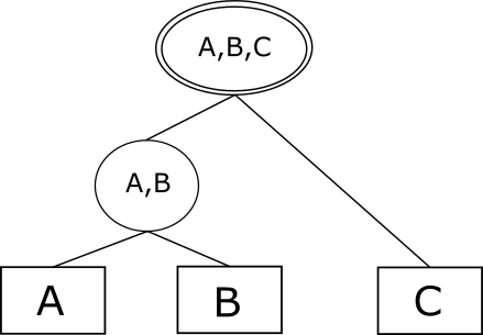
(a)

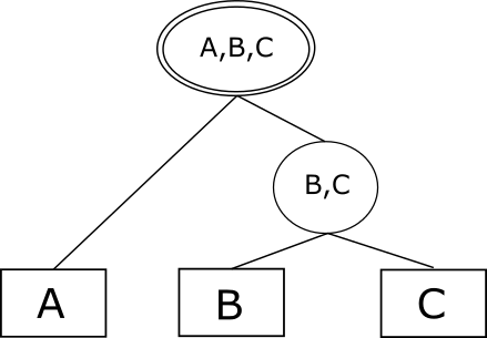
(b)

(c)

Figure 3: Evaluation trees for a pattern SEQ(A,B,C): LABEL:sub@fig:zstream-abc-left a left-deep tree produced by ZStream; LABEL:sub@fig:zstream-abc-right a right-deep tree produced by ZStream; LABEL:sub@fig:zstream-abc-reordering an optimal evaluation tree, which cannot be produced by ZStream.

3 Plan Generation Problems

This section defines and describes the two problems whose relationship will be closely studied in the subsequent sections. We start by presenting the CEP Plan Generation problem and explain its two variations, order-based CPG and tree-based CPG. Then, we briefly outline the Join Query Plan Generation (JQPG) problem.

3.1 CEP Plan Generation

We will start with the definition of the CEP evaluation plan. The evaluation plan provides a scheme for the evaluation mechanism, according to which its internal pattern representation is created. Therefore, different evaluation plans are required for different CEP frameworks. In this paper, we distinguish between two main types of plans, the order-based plan and the tree-based plan, with more complex types left for future work.

An order-based plan consists of a permutation of the primitive event types declared by the pattern. An order-based CEP engine uses this plan to set the order in which events are processed at runtime. Order-based plans are applicable to mechanisms evaluating a pattern event-by-event, as described in Section 2.2.

A tree-based plan extends the above by providing a tree-like scheme for pattern evaluation. In this scheme, the structure of the internal nodes serves as a loose order in which different events are to be matched. It specifies which subsets of valid matches are to be locally buffered and how to combine them into larger partial matches. Plans of this type can be used for the tree-based evaluation mechanism presented in Section 2.3.

We can thus define two variations of the CEP Plan Generation problem, order-based CPG and tree-based CPG. In each variation, the goal is to determine an optimal evaluation plan $P$ subject to some cost function $Cost\left(P\right)$. Different CEP systems define different metrics to measure their efficiency. In this paper we will consider a highly relevant performance optimization goal: reducing the number of active partial matches within the time window (denoted below simply as number of partial matches).

Regardless of the system-specific performance objectives, the implicit requirement to monitor all valid subsets of primitive events can become a major bottleneck. Because any partial match might form a full pattern match, their number is worst-case exponential in the number of events participating in a pattern. Further, as a newly arrived event needs to be checked against all (or most of) the currently stored partial matches, the processing time and resource consumption per event can become impractical for real-time applications. Other metrics, such as detection latency or network communication cost, may also be negatively affected. Thus, given the crucial role of the number of partial matches in all aspects of CEP, it was chosen as our primary cost function.

The formal definitions of the cost functions for order-based CPG and tree-based CPG will be given in Sections 4.1 and 4.2 respectively.

3.2 Join Query Plan Generation

Join Query Plan Generation is a well-known problem in query optimization [31, 45, 47]. In this problem, we are given relations $R_{1},\cdots,R_{n}$ and a query graph describing the mutual conditions to be satisfied by the tuples of the relations in order to be included in the result. A condition between any pair of relations $R_{i},R_{j}$ has a known selectivity $f_{i,j}\in\left[0,1\right]$ (we define $f_{i,j}=1$ if no such condition is defined between the two). The goal is to produce a query plan for this join operation, such that a predefined cost function defined on the plan space will be minimized.

One popular choice for the cost function is the number of intermediate tuples produced during plan execution. For the rest of this paper, we will refer to it as the intermediate results size. In [13], the following expression is given to calculate this function for each two-way join of two input relations:

$$C\left(R_{i},R_{j}\right)=\left|R_{i}\right|\cdot\left|R_{j}\right|\cdot f_{i,j},$$

where $\left|R_{i}\right|,\left|R_{j}\right|$ are the cardinalities of the joined relations. This formula is naturally extended to relations produced during join calculation:

$$C\left(S,T\right)=\left|S\right|\cdot\left|T\right|\cdot f_{S,T}.$$

Here, $S=R_{i_{1}}\bowtie\cdots\bowtie R_{i_{s}};T=R_{j_{1}}\bowtie\cdots\bowtie R_{j_{t}}$ are the partial join results of some subsets of $R_{1},\cdots,R_{n}$ and

$$f_{S,T}=\left|S\bowtie T\right|/\left|S\times T\right|$$

is the product of selectivities of all predicates defined between the individual relations comprising $S$ and $T$.

The two most popular classes of join query plans are the left-deep trees and the bushy trees. Algorithms based on the former type restrict their output to plans with a so-called “left-deep” topology. This type of join tree processes the input relations one-by-one, adding a new relation to the current intermediate result during each step. Hence, for this class of techniques, a valid solution is a join order rather than a join plan, since for any order over $R_{1},\cdots,R_{n}$ there exists exactly one left-deep tree. Figure 2LABEL:sub@fig:left-deep-tree depicts an example of a left-deep tree for a join query of four relations.

Approaches based on bushy trees pose no limitations on the plan topology, allowing it to contain arbitrary branches. An example is shown in Figure 2LABEL:sub@fig:bushy-tree. Here a valid solution specifies a complete join tree rather than merely an order.

In Sections 4.1 and 4.2 we will provide the formal definitions of the execution plan costs for left-deep and bushy join trees, respectively. The join query plan generation problem was shown by multiple authors to be NP-complete [13, 24], even when only left-deep trees are considered.

4 The Equivalence of CPG and JQPG for Pure Conjunctive Patterns

This section presents the formal proof of equivalence between CPG and JQPG for pure conjunctive patterns. We show that, when the pattern to be monitored is a pure conjunctive pattern and the CPG cost function represents the number of partial matches, the two problems are equivalent. From this result, we deduce the NP-completeness of CPG. In Section 5 we demonstrate how to convert non-pure sequence and conjunctive patterns to pure conjunctive form, thus proving that an instance of CPG for these pattern types can be reduced to an instance of JQPG (though the opposite does not hold).

4.1 Order-Based Evaluation

We will first focus on a CPG variation for order-based evaluation plans. In this section we will show that this problem is equivalent to JQPG restricted to left-deep trees. To that end, we will define the cost model functions for both problems and then present the equivalence theorem.

Our cost function $Cost_{ord}$ will reflect the number of partial matches coexisting in memory within the time window. The calculations will be based on the arrival rates of the events and the selectivities of the predicates.

Let $sel_{i,j}$ denote the selectivity of $c_{i,j}$, i.e., the probability of a partial match containing instances of events of types $T_{i}$ and $T_{j}$ to pass the condition. Additionally, let $r_{1},\cdots r_{n}$ denote the arrival rates of corresponding event types $T_{1},\cdots T_{n}$. Then, the expected number of primitive events of type $T_{i}$ arriving within the time window $W$ is $W\cdot r_{i}$. Let $O=\left(T_{p_{1}},T_{p_{2}},\cdots T_{p_{n}}\right);p_{i}\in[1,n]$ denote an execution order. Then, during pattern evaluation according to $O$, the expected number of partial matches of length $k,1\leq k\leq n$ is given by:

$$PM\left(k\right)=W^{k}\cdot\prod_{i=1}^{k}r_{p_{i}}\cdot\prod_{i,j\leq k;i\leq j}sel_{p_{i},p_{j}}.$$

The overall cost function we will attempt to minimize is thus the sum of partial matches of all sizes, as follows:

$$Cost_{ord}\left(O\right)=\sum_{k=1}^{n}\left(W^{k}\cdot\prod_{i=1}^{k}r_{p_{i}}\cdot\prod_{i,j\leq k;i\leq j}sel_{p_{i},p_{j}}\right).$$

For the JQPG problem restricted to output left-deep trees only, we will use the two-way join cost function $C\left(S,T\right)$ defined in Section 3.2. Let $L$ be a left-deep tree and let $\left\{i_{1},i_{2},\cdots,i_{n}\right\}$ be the order in which input relations are to be joined according to $L$. Let $P_{k},1\leq k<n$ denote the result of joining the first $k$ tables by $L$ (that is, $P_{1}=R_{i_{1}}$, $P_{2}=R_{i_{1}}\bowtie R_{i_{2}}$, etc.). In addition, let $C_{1}=\left|R_{i_{1}}\right|\cdot f_{i_{1},i_{1}}$ be the cost of the initial selection from $R_{i_{1}}$. Then, the cost of $L$ will be defined according to a left-deep join (LDJ) cost function:

$$Cost_{LDJ}\left(L\right)=C_{1}+\sum_{k=2}^{n}C\left(P_{k-1},R_{i_{k}}\right).$$

We are now ready to formally prove the statement formulated in the beginning of the section.

Theorem 1

Given a pure conjunctive pattern $P$, the problem of finding an order-based evaluation plan for $P$ minimizing $Cost_{ord}$ is equivalent to the Join Query Plan Generation problem for left-deep trees subject to $Cost_{LDJ}$.

We will start by proving that $CPG\subseteq JQPG$. To that end, we will present the corresponding reduction.

Given a pure conjunctive pattern $P$ defined as follows:

$$\begin{array}[]{l}\texttt{PATTERN AND}\left(T_{1}\>e_{1},\cdots T_{n}\>e_{n}\right)\\ \texttt{WHERE }\left(c_{1,1}\wedge c_{1,2}\wedge\cdots\wedge c_{n-1,n}\wedge c_{n,n}\right)\\ \texttt{WITHIN\> W,}\end{array}$$

let $R_{1},\cdots,R_{n}$ be a set of relations such that each $R_{i}$ corresponds to an event type $T_{i}$. For each attribute of $T_{i}$, including the timestamp, a matching column will be defined in $R_{i}$. The cardinality of $R_{i}$ will be set to $W\cdot r_{i}$, and, for each predicate $c_{i,j}$ with selectivity $sel_{i,j}$, an identical predicate will be formed between the relations $R_{i}$ and $R_{j}$. We will define the query corresponding to $P$ as follows:

$$\begin{array}[]{l}\texttt{SELECT *}\\ \texttt{FROM }R_{1},\cdots R_{n}\\ \texttt{WHERE }\left(c_{1,1}\texttt{ AND}\cdots\texttt{AND }c_{n,n}\right).\\ \end{array}$$

We will show that a solution to this instance of the JQPG problem is also a solution to the initial CPG problem. Recall that a left-deep JQPG solution $L$ minimizes the function $Cost_{LDJ}$. By opening the recursion and substituting the parameters with those of the original problem, we get:

$$Cost_{LDJ}\left(L\right)=C_{1}+\sum_{k=2}^{n}C\left(P_{k-1},R_{i_{k}}\right)=$$

$$= \left|R_{i_{1}}\right|\cdot f_{i_{1},i_{1}}+\sum_{k=2}^{n}\left(\prod_{j=1}^{k}\left|R_{i_{j}}\right|\cdot\prod_{j.l\leq k;j\leq l}f_{i_{j},i_{l}}\right)=$$

$$= \sum_{k=1}^{n}\left(\prod_{j=1}^{k}\left(W\cdot r_{i_{j}}\right)\cdot\prod_{j.l\leq k-1;j\leq l}sel_{i_{j},i_{l}}\right)=Cost_{ord}\left(O\right).$$

Consequently, the solution that minimizes $Cost_{LDJ}$ also minimizes $Cost_{ord}$, which completes the proof of the first direction of the theorem.

We will now proceed to proving the second direction, i.e., $JQPG\subseteq CPG$. Let $R_{1},\cdots,R_{n}$ be the relations to be joined with mutual predicates $F_{i,j}$ of selectivities $f_{i,j}$. We will demonstrate a decomposition of this problem to an instance of the CPG problem.

Let $T_{1},\cdots,T_{n}$ be primitive event types such that each $T_{i}$ corresponds to a relation $R_{i}$. Let each instance of $T_{i}$ have the attributes identical to the columns of $R_{i}$. In addition, let $S$ be an input stream containing a primitive event $t_{i,k}$ of type $T_{i}$ for each tuple $k$ of a relation $R_{i}$, where $1\leq k\leq\left|R_{i}\right|$ is an index of a tuple in a relation. Let the timestamp of each such event be defined as $t_{i,k}.ts=k$. Define the time window as $W=max\left|R_{i}\right|$, where $\left|R_{i}\right|$ is the cardinality of $R_{i}$. Finally, let $r_{i}$, the arrival rate of events of type $T_{i}$, be equal to $\frac{\left|R_{i}\right|}{W}$.

Now we are ready to define a CEP conjunctive pattern corresponding to the join of $R_{1},\cdots,R_{n}$, as follows:

$$\begin{array}[]{l}\texttt{PATTERN AND}\left(T_{1}\>e_{1},\cdots T_{n}\>e_{n}\right)\\ \texttt{WHERE }\left(F_{1,1}\wedge F_{1,2}\wedge\cdots\wedge F_{n-1,n}\wedge F_{n,n}\right)\\ \texttt{WITHIN\> W.}\end{array}$$

We will show that a solution to this instance of the CPG problem is also a solution to the initial JQPG problem. Recall that such a solution $O$ minimizes the function $Cost_{ord}$. By substituting the parameters with those of the original problem, we get:

$$Cost_{ord}\left(O\right)=\sum_{k=1}^{n}\left(W^{k}\cdot\frac{\prod_{i=1}^{k}\left|R_{p_{i}}\right|}{W^{k}}\cdot\prod_{i,j\leq k;i\leq j}f_{p_{i},p_{j}}\right)=$$

$$= \sum_{k=1}^{n}\left(\left(\prod_{i=1}^{k-1}\left|R_{p_{i}}\right|\cdot\prod_{i,j\leq k-1;i\leq j}f_{p_{i},p_{j}}\right)\cdot\left|R_{p_{k}}\right|\cdot\prod_{i\leq k}f_{p_{i},p_{k}}\right).$$

Here, the first sub-expression inside the summation is the intermediate results size until the point when the $k^{th}$ relation is to be joined, as follows from the definition above. The second sub-expression is the cardinality of the relation $R_{p_{k}}$, and the third sub-expression is the product of all predicates to be applied on tuples from $R_{p_{k}}$ upon joining it with $R_{p_{1}},\cdots R_{p_{k-1}}$. Therefore, the resulting expression is identical to $Cost_{LDJ}$ (in particular, the first element of the summation equals $C_{1}$). Consequently, the solution that minimizes $Cost_{ord}$ also minimizes $Cost_{LDJ}$, which completes the proof.$\blacksquare$

In [13] the authors showed the problem of Join Query Plan Generation for left-deep trees to be NP-complete for the general case of arbitrary query graphs. From this result and from the above theorem we will deduce the following corollary.

Corollary 1

The problem of finding an order-based evaluation plan for a general pure conjunctive complex event pattern that minimizes $Cost_{ord}$ is NP-complete.

4.2 Tree-Based Evaluation

In this section, we will extend Theorem 1 to tree-based evaluation plans. This time we will consider the unrestricted JQPG problem, allowed to return bushy trees. Similarly to the previous section, we will start by defining the cost functions and then proceed to the proof of the extended theorem.

We will define the cost model for evaluation trees in a manner similar to Section 4.1. We will estimate the number of partial matches accumulated in each node of the evaluation tree and sum them up to produce the cost function.

For a leaf node $l$ collecting events of type $T_{i}$, the expected number of partial matches is equal to the number of events of type $T_{i}$ arriving inside a time window:

$$PM(l)=W\cdot r_{i}.$$

To obtain an estimate for an internal node $in$, we multiply the cost function values of its children by the total selectivity of the predicates verified by this node:

$$PM(in)=PM\left(in.left\right)\cdot PM\left(in.right\right)\cdot SEL_{LR}\left(in\right),$$

where $SEL_{LR}$ is the selectivity of the predicates defined between event types accepted at the left and the right sub-trees of node $in$, or, more formally:

$$SEL_{LR}\left(in\right)=\prod_{\begin{array}[]{c}e_{i}\in in.ltree;e_{j}\in in.rtree\end{array}}sel_{i,j}.$$

The total cost function on a tree $T$ is thus defined as follows:

$$Cost_{tree}\left(T\right)=\sum_{N\in nodes\left(T\right)}PM\left(N\right).$$

For bushy trees, we will extend the cost function defined in Section 4.1. The cost of a tree node $N$ will be defined as follows:

$$C\left(N\right)=\begin{cases}\left|R_{i}\right|&N\>is\>a\>leaf\>representing\>R_{i}\\ \left|L\right|\cdot\left|R\right|\cdot f_{L,R}&N\>is\>an\>internal\>node\>representing\\ &a\>sub-join\>L\bowtie R,\end{cases}$$

with the bushy join (BJ) cost function defined as follows:

$$Cost_{BJ}\left(T\right)=\sum_{N\in nodes\left(T\right)}C\left(N\right).$$

We will now extend Theorem 1 to tree-based plans.

Theorem 2

Given a pure conjunctive pattern $P$, the problem of finding a tree-based evaluation plan for $P$ minimizing $Cost_{tree}$ is equivalent to the Join Query Plan Generation problem subject to $Cost_{BJ}$.

To prove the theorem, we decompose each of the tree cost functions $Cost_{tree},Cost_{BJ}$ defined above for the CPG and the JQPG problems into two components, separately calculating the cost of the leaves and the internal nodes:

$$Cost_{tree}^{l}\left(T\right)=\sum_{N\in leaves\left(T\right)}PM\left(N\right)$$

$$Cost_{tree}^{in}\left(T\right)=\sum_{N\in in\_nodes\left(T\right)}PM\left(N\right)$$

$$Cost_{BJ}^{l}\left(T\right)=\sum_{N\in leaves\left(T\right)}C\left(N\right)$$

$$Cost_{BJ}^{in}\left(T\right)=\sum_{N\in\ in\_nodes\left(T\right)}C\left(N\right).$$

Obviously, the following equalities hold:

$$Cost_{tree}\left(T\right)=Cost_{tree}^{l}\left(T\right)+Cost_{tree}^{in}\left(T\right)$$

$$Cost_{BJ}\left(T\right)=Cost_{BJ}^{l}\left(T\right)+Cost_{BJ}^{in}\left(T\right).$$

Thus, it is sufficient to prove that

$$Cost_{tree}^{l}\left(T\right)=Cost_{BJ}^{l}\left(T\right)$$

$$Cost_{tree}^{in}\left(T\right)=Cost_{BJ}^{in}\left(T\right).$$

for every $T$. From here it will follow that the solution minimizing $Cost_{tree}$ will also minimize $Cost_{BJ}$ and vice versa.

Applying either direction of the reduction from Theorem 1, we observe the following for the first pair of functions:

$$Cost_{tree}^{l}\left(T\right)=\sum_{N\in leaves\left(T\right)}PM\left(N\right)=\sum_{i=1}^{n}W\cdot r_{i}=\\ =\sum_{i=1}^{n}\left|R_{i}\right|=\sum_{N\in leaves\left(T\right)}C\left(N\right)=Cost_{BJ}^{l}\left(T\right).$$

Similarly, for the second pair of functions:

$$Cost_{tree}^{in}\left(T\right)=\sum_{N\in in\_nodes\left(T\right)}PM\left(N\right)=\\ =\sum_{N\in in\_nodes\left(T\right)}PM\left(N.left\right)\cdot PM\left(N.right\right)\cdot SEL_{LR}\left(N\right).$$

Opening the recursion, we get:

$$Cost_{tree}^{in}\left(T\right)=\sum_{N\in in\_nodes\left(T\right)}\left(\prod_{m\in leaves\left(N\right)}W\cdot r_{m}\cdot\prod_{i,j\in leaves\left(N\right)}sel_{i,j}\right).$$

By applying an identical transformation on $Cost_{JB}^{in}$ we obtain the following:

$$Cost_{BJ}^{in}\left(T\right)=\sum_{N\in in\_nodes\left(T\right)}\left(\prod_{m\in leaves\left(N\right)}\left|R_{m}\right|\cdot\prod_{i,j\in leaves\left(N\right)}f_{i,j}\right).$$

After substituting $r_{m}=\frac{\left|R_{m}\right|}{W}$ and $sel_{p_{i},p_{j}}=f_{p_{i},p_{j}}$, the two expressions are identical, which completes the proof.$\blacksquare$

The CPG-JQPG reduction that we will use for tree-based evaluation is the one demonstrated in Theorem 1 for order-based evaluation.

By Theorem 2 and the generalization of the result in [13], we derive the following corollary.

Corollary 2

The problem of finding a tree-based evaluation plan for a general pure conjunctive complex event pattern that minimizes $Cost_{tree}$ is NP-complete.

4.3 Join Query Types

As Corollaries 1 and 2 imply, no efficient algorithm can be devised to optimally solve CPG for a general conjunctive pattern unless $P=NP$. However, better complexity results may be available under certain assumptions regarding the pattern structure. Numerous works considered the JQPG problem for restricted query types, that is, specific topologies of the query graph defining the inter-relation conditions. Examples of such topologies include clique, tree, and star.

It was shown in [24, 31] that an optimal plan can be computed in polynomial time for left-deep trees and queries forming an acyclic graph (i.e., tree queries), provided that the cost function has the ASI (adjacent sequence interchange) property [37]. The left-deep tree cost function $Cost_{LDJ}$ has this property [13], making the result applicable for our scenario. A polynomial algorithm without the ASI requirement was proposed for bushy tree plans for chain queries [39]. From Theorems 1 and 2 we can conclude that, for conjunctive patterns only, CPG$\in$P under the above constraints.

However, these results only hold when the plans produced by a query optimizer are not allowed to contain cross products [13, 39]. While this limitation is well-known in relational optimization [49], it is not employed by the existing CPG methods [6, 29, 35, 44]. Moreover, it was shown that when cross products are omitted, cheaper plans might be missed [38]. Thus, even when an exact polynomial algorithm is applicable to CPG, it is inferior to native algorithms in terms of the considered search space and can only be viewed as a heuristic. In that sense, it is similar to the greedy and randomized approaches [46, 47].

Other optimizations utilizing the knowledge of the query type were proposed. For example, the optimal bushy plan was empirically shown to be identical to the optimal left-deep plan for star queries and, in many cases, for grid queries [46]. This observation allows us to utilize a cheaper left-deep algorithm for the above query types without compromising the quality of the resulting plan.

With the introduction of additional pattern types (Section 5) and event selection strategies (Section 6.2), new query graph topologies might be identified and type-specific efficient algorithms designed. This topic is beyond the scope of this paper and is a subject for future work.

Although not used directly by the JQPG algorithms, the order-based CPG cost functions $Cost_{ord}$ and $Cost_{ord}^{lat}$ (that we will introduce in Section 6.1) also have the ASI property. We formally prove this statement in the Appendix A.

5 JQPG for General Pattern Types

The reduction from CPG to JQPG presented above only applies to pure conjunctive patterns. However, the patterns encountered in real-world scenarios are much more diverse. To complete the solution, we have to consider simple patterns containing SEQ, OR, NOT and KL operators. We also have to address nested patterns.

This section describes how a pattern of each of the aforementioned types can be represented and detected as either a pure conjunctive pattern or their union. To that end, we will utilize some of the ideas from [28]. Note that the transformations presented below are only applied for the purpose of plan generation, that is, no actual conversion takes place during execution on a data stream.

5.1 Sequence patterns

We observe that a sequence pattern is merely a conjunctive pattern with additional temporal constraints, i.e., predicates on the values of the timestamp attribute. Thus, a general pure sequence pattern of the form

$$\begin{array}[]{l}PATTERN\>SEQ\left(T_{1}\>e_{1},T_{2}\>e_{2},\cdots,T_{n}\>e_{n}\right)\\ WHERE\>(c_{1,1}\wedge c_{1,2}\wedge\cdots\wedge c_{n,n-1}\wedge c_{n,n})\\ WITHIN\>W\end{array}$$

can be rewritten in the following way without any change in the semantics:

$$\begin{array}[]{l}PATTERN\>AND\left(T_{1}\>e_{1},T_{2}\>e_{2},\cdots,T_{n}\>e_{n}\right)\\ WHERE\>(c_{1,1}\wedge\cdots\wedge c_{n,n}\wedge\\ \qquad\qquad\wedge\left(e_{1}.ts<e_{2}.ts\right)\wedge\cdots\wedge\left(e_{n-1}.ts<e_{n}.ts\right))\\ WITHIN\>W.\end{array}$$

An instance of the sequence pattern is thus reduced from CPG to JQPG similarly to a conjunctive pattern, with the timestamp column added to each relation $R_{i}$ representing an event type $T_{i}$, and constraints on the values of this column introduced into the query representation.

We will now formally prove the correctness of the above construction.

Theorem 3

Let $S$ be a pure sequence pattern specified by primitive event types $T_{1},\cdots,T_{n}$, a Boolean predicate of constraints $P_{S}=\bigwedge_{1\leq i,j\leq n}c_{i,j}$, and a time window $W$. Additionally, let $C$ be a pure conjunctive pattern specified by $T_{1},\cdots,T_{n}$, a time window $W^{\prime}=W$, and a predicate $P_{C}=P_{S}\wedge P_{O}$, where $P_{O}=\bigwedge_{1\leq i<n}\left(e_{i}.ts<e_{i+1}.ts\right)$. Then, $S$ is equivalent to $C$, i.e., both patterns specify the same set of matches.

We will prove this theorem by double inclusion.

$S\subseteq C$: Let $M=\left\{e_{1},\cdots,e_{n}\right\}$ be a match for $S$. Then, by definition, $M$ satisfies $P_{S}$. In addition, since $S$ is a sequence pattern, events in $M$ follow the temporal order $e_{1}.ts<e_{2}.ts<\cdots<e_{n}.ts$. Hence, $M$ also satisfies $P_{O}$, and thus $P_{C}$ as well, i.e., $M$ is a match for $C$.

$C\subseteq S$: Let $M=\left\{e_{1},\cdots,e_{n}\right\}$ be a match for $C$. Since $M$ satisfies $P_{O}$, its events satisfy the ordering constraints $e_{1}.ts<\cdots<e_{n}.ts$. By definition of a sequence pattern, $\left\{e_{1},\cdots,e_{n}\right\}$ form a valid sequence within the time window $W$. Additionally, $M$ satisfies $P_{S}$. Hence, by definition, $M$ is a match for $S$.$\blacksquare$

5.2 Kleene closure patterns

In a pattern with an event type $T_{i}$ under a KL operator, any subset of events of $T_{i}$ within the time window can participate in a match. During plan generation, we are interested in modeling this behavior in a way comprehensible by a JQPG algorithm, that is, using an equivalent pattern without Kleene closure. To that end, we introduce a new type $T_{i}^{\prime}$ to represent all event subsets accepted by $KL\left(T_{i}\right)$, that is, the power set of events of $T_{i}$. A set of $k$ events of type $T_{i}$ will be said to contain $2^{k}$ “events” of type $T_{i}^{\prime}$, one for each subset of the original $k$ events. The new pattern is constructed by replacing $KL\left(T_{i}\right)$ with $T_{i}^{\prime}$. Since a time window of size $W$ contains $2^{r_{i}\cdot W}$ subsets of $T_{i}$ (where $r_{i}$ is the arrival rate of $T_{i}$), the arrival rate $r{}_{i}^{\prime}$ of $T_{i}^{\prime}$ is set to $\frac{2^{r_{i}\cdot W}}{W}$. The predicate selectivities remain unchanged.

For example, given the following pattern with the arrival rate of 5 events per second for each event type:

$$\begin{array}[]{l}\texttt{PATTERN AND(A a,KL(B b),C c)}\\ \texttt{WHERE ({true}) WITHIN 10 seconds,}\end{array}$$

the pattern to be utilized for plan generation will be:

$$\begin{array}[]{l}\texttt{PATTERN AND(A a,B' b,C c)}\\ \texttt{WHERE ({true}) WITHIN 10 seconds.}\end{array}$$

The arrival rate of $B^{\prime}$ will be calculated as $r_{B}^{\prime}=\frac{2^{r_{B}\cdot W}}{W}=\frac{1}{10}\cdot 2^{50}$. A plan generation algorithm will then be invoked on the new pattern. Due to an extremely high arrival rate of $B^{\prime}$, its processing will likely be postponed to the latest step in the plan, which is also the desired strategy for the original pattern in this case. $B^{\prime}$ will then be replaced with $B$ in the resulting plan, and the missing Kleene closure operator will be added in the respective stage (by modifying an edge type for a NFA [28] or a node type for a tree [35]), thus producing a valid plan for detecting the original pattern. We will now formally prove the correctness of the above construction.

Theorem 4

Let $K$ be a conjunctive pattern specified by primitive event types $T_{1},\cdots,T_{i},\cdots,T_{n}$, a Boolean predicate of constraints $P_{K}=\bigwedge_{1\leq i,j\leq n}c_{i,j}$, and a time window $W$. In addition, let $K$ contain a Kleene closure operator applied on an event type $T_{i}$. Let a new type $T_{i}^{\prime}$ represent the power set of events of the type $T_{i}$, i.e., for each set of events $\left\{e_{i}^{1},e_{i}^{2},\cdots,e_{i}^{k}\right\}$ of type $T_{i}$ within the time window an event of type $T{}_{i}^{\prime}$ is created, containing each of $e_{i}^{j}$ as an attribute. Let $C$ be a pure conjunctive pattern specified by $T_{1},\cdots,T_{i}^{\prime},\cdots,T_{n}$, a predicate $P{}_{C}=P_{K}$, and a time window $W^{\prime}=W$. Then, $K$ is equivalent to $C$, i.e., both patterns specify the same set of matches.

We will show that for an arbitrary input stream both patterns will produce identical sets of pattern matches. Let $S=\left\{s_{1},\cdots,s_{m}\right\}$ be an input stream. W.l.o.g., assume that each event in $S$ belongs to one of the types $T_{1},\cdots,T_{n}$ and that all events are within the time window $W$. Additionally, let $S^{\prime}\subset S$ denote the set of all events of type $T_{i}$ in $S$. Then, while monitoring the pattern $K$, the system will create $2^{\left|S^{\prime}\right|}-1$ partial matches for each unique combination of events of types $T_{1},\cdots,T_{i-1},T_{i+1},\cdots,T_{n}$.

Now, let $S^{\prime\prime}\subset S$ denote the set of all events of type $T{}_{i}^{\prime}$ in $S$. While monitoring $C$, for each combination of events of types $T_{1},\cdots,T_{i-1},T_{i+1},\cdots,T_{n}$ the detecting framework will create $\left|S^{\prime\prime}\right|$ partial matches, one for each primitive event in $S^{\prime\prime}$. For each non-empty subset of $S^{\prime}$, $S^{\prime\prime}$ contains an event corresponding to this subset, and vice versa. As the constraints on both patterns are identical, as well as the time window, the resulting full matches will also be the same.$\blacksquare$

Corollary 3

Theorem 4 holds also for sequence patterns.

The correctness of this corollary follows from the transitivity of conversions in Theorems 3 and 4.

Corollary 4

Theorem 4 and Corollary 3 hold for an arbitrary number of non-nested Kleene closure operators in a pattern.

The proof of this corollary is by iteratively applying Theorem 4 or Corollary 3 on each Kleene closure operator.

5.3 Negation patterns

Patterns with a negated event will not be rewritten. Instead, we will introduce a negation-aware evaluation plan creation strategy. First, a plan will be generated for a positive part of a pattern as described above. Then, a check for the appearance of a negated event will be added at the earliest point possible, when all positive events it depends on are already received. This construction process will be implemented by augmenting a plan with a transition to the rejecting state for a NFA [28] or with a NSEQ node for a ZStream tree [35]. For example, given a pattern $SEQ\left(A,NOT\left(B\right),C,D\right)$, the existence of a matching $B$ in the stream will be tested immediately after the latest of $A$ and $C$ have been accepted. Since both Lazy NFA and ZStream incorporate event buffering, this technique is feasible and easily applicable.

5.4 Nested patterns

Patterns of this type can contain an unlimited number of n-ary operators. After transforming SEQ to AND as shown above, we are left with only two such operator types, AND and OR. Given a nested pattern, we convert the pattern formula to DNF form, that is, an equivalent nested disjunctive pattern containing a list of simple conjunctive patterns is produced. Then, a separate evaluation plan is created for each conjunctive subpattern, and their detection proceeds independently. The returned result is the union of all subpattern matches.

Note that applying the DNF transformation can cause some expressions to appear in multiple subpatterns. For example, a nested pattern of the form $AND\left(A,B,OR\left(C,D\right)\right)$ will be converted to a disjunction of conjunctive patterns $AND\left(A,B,C\right)$ and $AND\left(A,B,D\right)$. As a result, redundant computations will be performed by automata or trees corresponding to different subpatterns (comparing $A$’s to $B$’s in our example). This problem can be solved by applying known multi-query techniques for shared subexpression processing, such as those described in [17, 34, 42, 43, 53].

6 Adapting JQPG Algorithms to
Complex Event Processing

The theoretical results from previous sections imply that any existing technique for determining a close-to-optimal execution plan for a join query can be adapted and used in CEP applications. However, many challenges arise when attempting to perform this transformation procedure in practice. First, despite the benefits of the cost function introduced in Section 3.1, simply counting the partial matches is not always sufficient. Additional performance metrics are often essential, such as the average response time. Second, complex event specification languages contain various constructs not present in traditional databases, such as event selection strategies. Third, the arrival rates of event types and the predicate selectivities are rarely obtained in advance and can change rapidly over time. A solution must be devised to measure the desired statistics on-the-fly and adapt the evaluation plan accordingly.

In this section, we show how detection latency and event selection strategies can be incorporated into existing JQPG algorithms. We also address the problem of adapting to dynamic changes in the input stream.

6.1 Pattern Detection Latency

Latency is commonly defined as a time difference between the arrival of the last primitive event comprising a full pattern match and the time of reporting this match by a CEP system. As many existing applications involve strong real-time requirements, pattern detection latency has become an important optimization goal for such systems. Unfortunately, in most cases it is impossible to simultaneously achieve maximal throughput and minimal latency, and trade-offs between the two are widely studied in the context of complex event processing [6, 51].

Detection schemes utilizing out-of-order evaluation, like those discussed in this paper, often suffer from increased latency as compared to more naïve approaches. The main reason is that, when an execution plan is optimized for maximal throughput, the last event in the pattern may not be the last event in the plan. After this event is accepted, the evaluation mechanism still needs to walk through the remaining part of the plan, resulting in late detection of the full match.

Algorithms adopted from JQPG do not naturally support latency. However, since they are generally independent of the cost model, this problem can be solved by providing an appropriate cost function. In addition to functions presented in Sections 4.1 and 4.2, which we will refer to as $Cost_{ord}^{trpt}$ and $Cost_{tree}^{trpt}$, a new pair of functions, $Cost_{ord}^{lat}$ and $Cost_{tree}^{lat}$, will reflect the expected latency of a plan. To combine the functions, many existing multi-objective query optimization techniques can be used, e.g., pareto optimal plan calculation [6] or parametric methods [48]. Systems with limited computational resources may utilize simpler and less expensive solutions, such as defining the total cost function as a weighted sum of its two components:

$$Cost\left(Plan\right)=Cost^{trpt}\left(Plan\right)+\alpha\cdot Cost^{lat}\left(Plan\right),$$

where $\alpha$ is a user-defined parameter adjusted to fit the required throughput-latency trade-off. This latter model was used during our experiments (Section 7).

We will now formally define the latency cost functions. For a sequence pattern, let $T_{n}$ denote the last event type in the order induced by the pattern. Then, for an order-based plan $O$, let $Succ_{O}\left(T_{n}\right)$ denote the event types succeeding $T_{n}$ in $O$. Following the arrival of an event of type $T_{n}$, in the worst case we need to examine all locally buffered events of types in $Succ_{O}\left(T_{n}\right)$. As defined in Section 4.1, there are $W\cdot r_{i}$ such events of type $T_{i}$, hence:

$$Cost_{ord}^{lat}\left(O\right)=\sum_{T_{i}\in Succ_{O}\left(T_{n}\right)}W\cdot r_{i}.$$

Similarly, for a tree-based plan $T$, let $Anc_{T}\left(T_{n}\right)$ denote all ancestor nodes of the leaf corresponding to $T_{n}$ in $T$, i.e., nodes located on a path from $T_{n}$ to the root (excluding the root). Let us examine the traversal along this path. When an internal node $N$ with two children $L$ and $R$ receives a partial match from, say, the child $L$, it compares this match to all partial matches currently buffered on $R$. Thus, the worst-case detection latency of a sequence pattern ending with $T_{n}$ is proportional to the number of partial matches buffered on the siblings of the nodes in $Anc_{T}\left(T_{n}\right)$. More formally, let $sibling\left(N\right)$ denote the other child of the parent of $N$ (for the root this function will be undefined). Then,

$$Cost_{tree}^{lat}\left(T\right)=\sum_{N\in Anc_{T}\left(T_{n}\right)}PM\left(sibling\left(N\right)\right).$$

For a conjunctive pattern, estimating the detection latency is a more difficult problem, as the last arriving event is not known in advance. One possible approach is to introduce a new system component, called the output profiler. The output profiler examines the full matches reported as output and records the most frequent temporal orders in which primitive events appear. Then, as enough information is collected, the latency function may be defined as in the previous case, subject to the event arrival order with the highest probability of appearance.

Finally, for a disjunctive pattern, we define the latency cost function as the maximum over the disjunction operands. This definitions applies also for arbitrary nested patterns.

6.2 Event Selection Strategies

In addition to event types, operators and predicates, CEP patterns are further defined using the event selection strategies [5, 16, 21] . An event selection strategy specifies how events are selected from an input stream for partial matches. In this section, we discuss four existing strategies and show how a reduction from JQPG to CPG can support them.

Until now, we have implicitly assumed the skip-till-any-match selection strategy [5], which permits a primitive event to participate in an unlimited number of matches. This strategy is the most flexible, as it allows all possible combinations of events comprising a match to be detected. However, some streaming applications do not require such functionality. Thus, additional strategies were defined, restricting the participation of an event in a match.

The skip-till-next-match selection strategy [5] limits a primitive event to appear in no more than a single full match. This is enforced by “consuming” events already assigned to a match. While this strategy prevents some matches from being discovered, it also considerably simplifies the detection process. In a CEP system operating under the skip-till-any-match policy, our cost model will no longer provide a correct estimate for a number of partial matches, which would lead to arbitrarily inefficient evaluation plans. However, since most JQPG algorithms do not depend on a specific cost function, we can solve this issue by replacing $Cost_{order}$ and $Cost_{tree}$ with newly devised models.

Let us examine the number of partial matches in an order-based setting under the skip-till-next-match strategy. We will denote by $m\left[k\right]$ the number of matches of size $k$ expected to exist simultaneously in a time window. Obviously, $m\left[1\right]=W\cdot r_{p_{1}}$, where $T_{p_{1}}$ is the first event type in the selected evaluation order. For the estimate of $m\left[2\right]$, there are two possibilities. If $r_{p_{1}}>r_{p_{2}}$, there will not be enough instances of $T_{p_{2}}$ to match all existing instances of $T_{p_{1}}$, and some of the existing matches of size 1 will never be extended. Hence, $m\left[2\right]=W\cdot r_{p_{2}}$ in this case. Otherwise, as an existing partial match cannot be extended by more than a single event of type $T_{p_{2}}$, $m\left[1\right]$ will be equal to $m\left[2\right]$. In addition, if a mutual condition exists between $T_{p_{1}}$and $T_{p_{2}}$, the resulting expression has to be multiplied by $sel_{p_{1},p_{2}}$.

By extending this reasoning to an arbitrary partial match, we obtain the following expression:

$$m\left[k\right]=W\cdot min\left(r_{p_{1}},r_{p_{2}},\cdots,r_{p_{k}}\right)\cdot\prod_{i,j\leq k;i\leq j}sel_{p_{i},p_{j}};\>1\leq k\leq n.$$

And the new cost function for order-based CPG is

$$Cost_{ord}^{next}\left(O\right)=\sum_{k=1}^{n}\left(W\cdot m\left[k\right]\right).$$

Using similar observations, we extend the above result for the tree-based model:

$$PM(n)=W\cdot min_{T_{i}\in subtree\left(n\right)}\left(r_{i}\right)\cdot\prod_{T_{i},T_{j}\in subtree\left(n\right)}sel_{i,j};$$

$$Cost_{tree}^{next}\left(T\right)=\sum_{n\in nodes\left(T\right)}PM\left(n\right).$$

The two remaining selection strategies, strict contiguity and partition contiguity [5], define further restrictions on the appearance of events in a match. The strict contiguity requirement forces the selected events to be contiguous in the input stream, i.e., it allows no other events to appear in between. The partition contiguity strategy is a slight relaxation of the above. It partitions the input stream according to some condition and only requires the events located in the same partition to be contiguous.

To support JQPG-based solutions for CPG under strict or partition contiguity, we will explicitly model the constraints imposed by the above strategies. In addition, the cost model presented earlier for skip-till-next-match will be used for both selection strategies.

To express strict contiguity, we will augment each primitive event with a new attribute reflecting its unique serial number in the stream. Then, we will add a new condition for each pair of potentially neighboring events, requiring the numbers to be adjacent.

For partition contiguity, the new attribute will represent an inner, per-partition order rather than a global one. Unless the partitioning condition is very costly to evaluate (which is rarely the case), this transformation can be efficiently and transparently applied on the input stream. The new contiguity condition will first compare the partition IDs of the two events, and only verify their serial numbers if the IDs match. We assume that the value distribution across the partitions remains unchanged. Otherwise, the evaluation plan is to be generated on a per-partition basis. Techniques incorporating per-partition plans are beyond the scope of this paper and are a subject for our future research.

6.3 Adaptive Complex Event Processing

As their definition implies, JQPG algorithms can only be used when event arrival rates and predicate selectivities are given in advance. However, in real-life scenarios this a priori knowledge is rarely available. Moreover, the data characteristics are subject to frequent on-the-fly fluctuations. To ensure efficient operation, a CEP engine must continuously estimate the current statistic values and, when a significant deviation is detected, adapt itself by recalculating the affected evaluation plans. Developing efficient adaptive mechanisms is considered a hard problem and a hot research topic in several fields [9, 19, 29, 35].

Due to the considerable generality, importance, and complexity of adaptive complex event processing, we devote a separate paper [27] to the discussion of this problem. In it, we propose a novel adaptivity mechanism and study it theoretically and empirically in conjunction with a JQPG-based evaluation plan generator.

7 Experimental Evaluation

In this section, we present our experimental study on real-world data. Our main goal was to compare some of the well-known JQPG algorithms, adapted for CPG as described above, to the currently used methods developed directly for CPG. The results demonstrate the superiority of the former in terms of quality and scalability of the generated plans.

In the following section we describe the algorithms compared during the study. Then we present the experimental setup, followed by the obtained results.

7.1 CPG and JQPG Algorithms

We implemented 5 order-based and 3 tree-based CPG algorithms. Out of those, 3 order-based and 2 tree-based algorithms are JQPG methods adapted to the CEP domain. Our main goal is to evaluate those algorithms against the rest, which are native CPG techniques. The order-based plan generation algorithms included the following:

• Trivial order (TRIVIAL) - the evaluation plan is set to the initial order of the sequence pattern. This strategy is used in various CEP engines based on NFAs, such as SASE [50] and Cayuga [18].

• Event frequency order (EFREQ) - the events are processed by the ascending order of their arrival frequencies. This is the algorithm of choice for frameworks such as PB-CED [6] and the Lazy NFA [29].

• Greedy cost-based algorithm (GREEDY) [47] - this greedy heuristic algorithm for JQPG proceeds by selecting at each step the relation which minimizes the value of the cost function. Here and below, unless otherwise stated, we will use cost functions minimizing the intermediate results size (Sections 4.1 and 4.2).

• Iterative improvement algorithm (II-RANDOM / II-GREEDY) - a local search JQPG algorithm, starting from some initial execution plan and attempting a set of moves to improve the cost function, until a local minimum is reached. In this study, we experimented with two variations of this algorithm, presented in [47]. The first, denoted as II-RANDOM, starts from a random order. The second, denoted as II-GREEDY, first applies a greedy algorithm to create an initial state. In both cases, the functions used to traverse between states are swap (the positions of two event types in a plan are swapped) and cycle (the positions of three event types are shifted).

• Dynamic programming algorithm for left-deep trees (DP-LD) - first presented in [45], this exponential-time algorithm utilizes dynamic programming to produce a provably optimal execution plan. The result is limited to a left-deep tree topology.

For the tree-based plan generation algorithms, the following were used:

• ZStream plan generation algorithm (ZSTREAM) - creates an evaluation tree by iterating over all possible tree topologies for a given sequence of leaves [35].

• ZStream with greedy cost-based ordering (ZSTREAM-ORD) - as was demonstrated in Section 2.3, the limitation of the ZStream algorithm is in its inability to modify the order of tree leaves. This algorithm attempts to utilize an order-based JQPG method to overcome this drawback. It operates by first executing GREEDY on the leaves of the tree to produce a ’good’ ordering, then applying ZSTREAM on the resulting list.

• Dynamic programming algorithm for bushy trees (DP-B) [45] - same as DP-LD, but without the topology restriction.

7.2 Experimental Setup

The data used during the experiments was taken from the NASDAQ stock market historical records [1]. In this dataset, each record represents a single update to the price of a stock, spanning a 1-year period and covering over 2100 stock identifiers with prices periodically updated. Our input stream contained 80,509,033 primitive events, each consisting of a stock identifier, a timestamp, and a current price. For each identifier, a separate event type was defined. In addition, we augmented the event format to include the difference between the current and the previous price of each stock. The differences were calculated during the preprocessing stage.

To compare a set of plan generation algorithms, we need to use them to create a set of evaluation plans for the same pattern and apply the resulting plans on the input data stream using a CEP platform of choice. To that end, we implemented two evaluation mechanisms discussed in this paper, the out-of-order lazy NFA [29] and the instance-based tree model based on ZStream [35] as presented in Section 2.3. The former was then used to evaluate plans created by each order-based CPG or JQPG algorithm on the patterns generated as described below. The latter was similarly used for comparing tree-based plans.

The majority of the experiments were performed separately on 5 sets of patterns: (1)pure sequences; (2)sequences with a negated event (marked as ’negation’ patterns in the graphs below); (3)conjunctions; (4)sequences containing an event under KL operator (marked as ’Kleene closure’ patterns); (5)composite patterns, consisting of a disjunction of three sequences (marked as ’disjunction’ patterns). Each set contained 500 patterns with the sizes (numbers of the participating events) ranging from 3 to 7, 100 patterns for each value. The pattern time window was set to 20 minutes.

The pattern structure was motivated by the problem of monitoring the relative changes in stock prices. Each pattern included a number of predicates, roughly equal to half the size of a pattern, comparing the difference attributes of two of the involved event types. For example, one pattern of size 3 from the set of conjunction patterns was defined as follows:

$$\begin{array}[]{l}PATTERN\>AND(\\ \qquad MSFT\textunderscore Stock\>m,GOOG\textunderscore Stock\>g,INTC\textunderscore Stock\>i)\\ WHERE\>(m.difference<g.difference)\\ WITHIN\>20\>minutes.\end{array}$$

The intention of this particular pattern is to examine the shift in the value of Intel’s stock in situations where Google’s stock price change is higher than Microsoft’s.

All arrival rates and predicate selectivities were calculated during the preprocessing stage. The measured arrival rates varied between 1 and 45 events per second, and the selectivities ranged from 0.002 to 0.88. As discussed in Section 6.3, in most real-life scenarios these statistics are not available in advance and may fluctuate frequently and significantly during runtime. We experimentally study the impact of these issues in a separate paper [27].

We selected throughput and memory consumption as our performance metrics for this study. Throughput was defined as the number of primitive events processed per second during pattern detection using the selected plan. To estimate the memory consumption, we measured the peak memory required by the system during evaluation. The metrics were acquired separately for each pattern, and the presented results were then calculated by taking the average.

All models and algorithms under examination were implemented in Java. The experiments were run on a machine with 2.20 Ghz CPU and 16.0 GB RAM and took about 1.5 months to complete.

7.3 Experimental Results

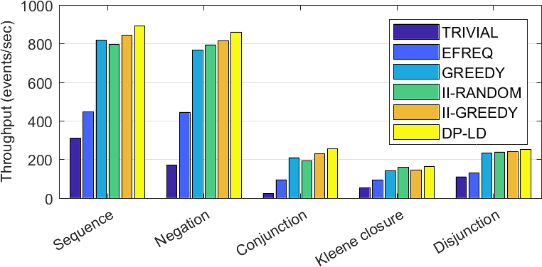
(a)

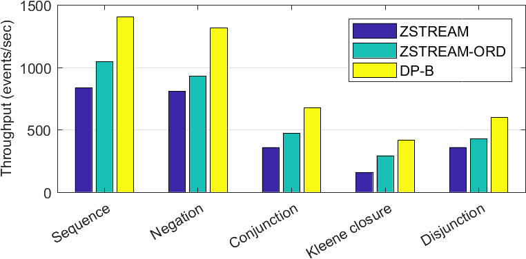
(b)

Figure 4: Throughput for different pattern types (higher is better): LABEL:sub@fig:throughput-order order-based methods; LABEL:sub@fig:throughput-tree tree-based methods.

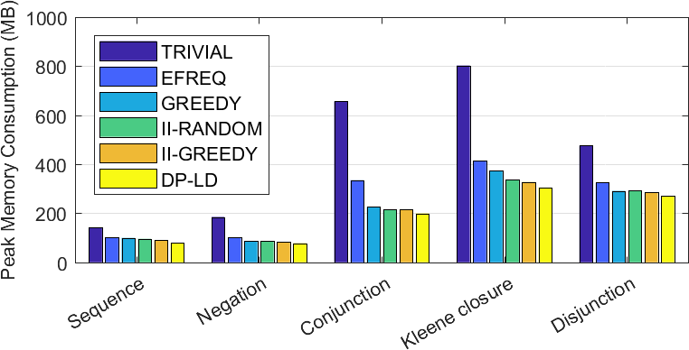
(a)

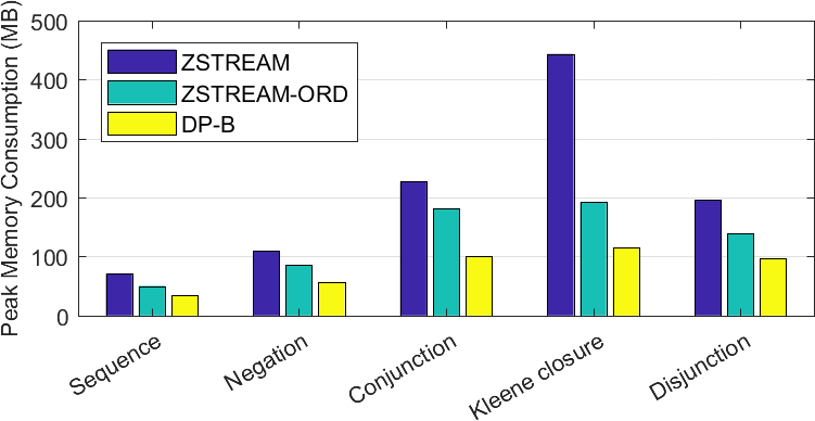
(b)

Figure 5: Memory consumption for different pattern types (lower is better): LABEL:sub@fig:memory-order order-based methods; LABEL:sub@fig:memory-tree tree-based methods.

Figures 4 and 5 present the comparison of the plan generation algorithms described in Section 7.1 in terms of throughput and memory consumption, respectively. Each group represents the results obtained on a particular set of patterns described above, and each bar depicts the average value of a performance metric for a particular algorithm. For clarity, order-based and tree-based methods are shown separately.

On average, the plans generated using JQPG algorithms achieve a considerably higher throughput than those created using native CPG methods. For order-based plans, the perceived gain of the best-performed DP-LD over EFREQ ranged from a factor of 1.7 for iteration patterns to 2.7 for conjunctions. Similar results were obtained for tree-based plans (ZSTREAM vs. DP-B). JQPG methods also display better overall memory utilization. The order-based JQPG plans consume about 65-85% of the memory required by those produced by EFREQ. An even greater difference was observed for tree-based plans, with DP-B using up to almost 4 times less memory than the CEP-native ZSTREAM.

Unsurprisingly, the best performance was observed for plans created using the exhaustive algorithms based on dynamic programming, namely DP-LD and DP-B. However, due to the exponential complexity of these algorithms, their use in practice may be problematic for large patterns, especially in systems where new evaluation plans are to be generated with high frequency. Thus, one goal of the experimental study was to test the exhaustive JQPG methods against the nonexhaustive ones (such as GREEDY and II algorithms) to see whether the performance gain of the former category is worth the high plan generation cost.

For the order-based case, the answer is indeed negative, as the results for DP-LD and the heuristic JQPG algorithms are comparable and no significant advantage is achieved by the former. Due to the relatively small size of the left-deep tree space, the heuristics usually succeed in locating the globally optimal plan. Moreover, the II-GREEDY algorithm generally produces plans that are slightly more memory-efficient. This can be attributed to our cost model, which only counts the partial matches, but does not capture the other factors such as the size of the buffered events. The picture looks entirely different for the tree-based methods, where DP-B displays a convincing advantage over both the basic ZStream algorithm and its combination with the greedy heuristic method.

Another important conclusion from Figures 4 and 5 is that methods following the tree-based model greatly outperform the order-based ones, both in throughput and memory consumption. This is not a surprising outcome, as the tree-based algorithms are capable of creating a significantly larger space of plans. However, the best order-based JQPG algorithm (DP-LD) is comparable or even superior to the CPG-native ZStream in most settings.

Figures 6-15 depict the results discussed above, partitioned by the pattern size. Throughput for each of the five pattern categories described above is displayed in Figures 6, 8, 10, 12, and 14 respectively. Although the performance of all methods degrades drastically as the pattern size grows, the relative throughput gain for JQPG methods over native CPG methods is consistently higher for longer sequences. This is especially evident for the tree-based variation of the problem (6LABEL:sub@fig:throughput-tree), where the most efficient JQPG algorithm (DP-B) achieves 7.6 times higher throughput than the native CPG framework (ZSTREAM) for patterns of length 7, compared to a speedup of only 1.2 times for patterns of 3 events. The results for memory consumption follow the same trend (Figures 7, 9, 11, 13, and 15). We can thus conclude that, at least for the pattern sizes considered in this study, the JQPG methods provide a considerably more scalable solution.

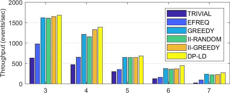
(a)

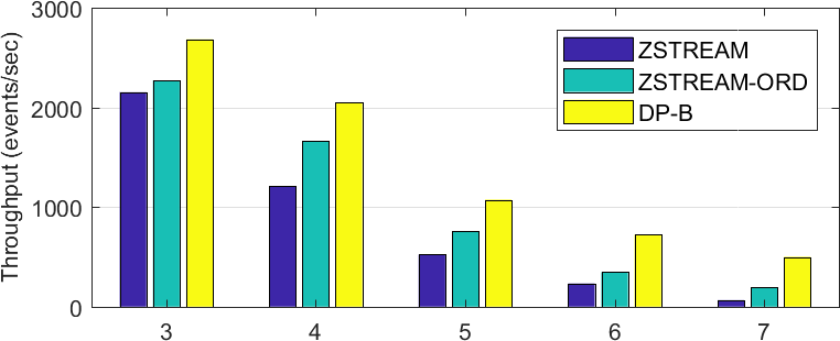
(b)

Figure 6: Throughput as a function of the sequence pattern size (higher is better): LABEL:sub@fig:throughput-order order-based methods; LABEL:sub@fig:throughput-tree tree-based methods.

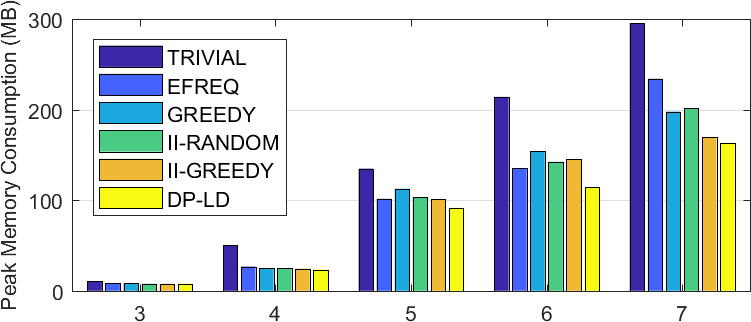
(a)

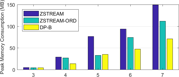
(b)

Figure 7: Memory consumption as a function of the sequence pattern size (lower is better): LABEL:sub@fig:memory-order order-based methods; LABEL:sub@fig:memory-tree tree-based methods.

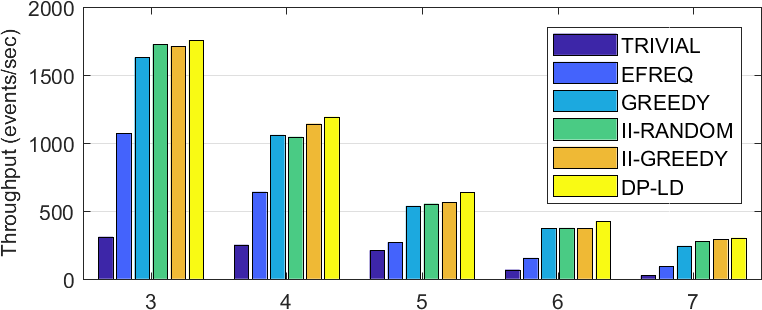
(a)

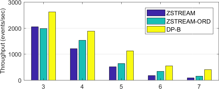
(b)

Figure 8: Throughput as a function of the negation pattern size (higher is better): LABEL:sub@fig:throughput-order order-based methods; LABEL:sub@fig:throughput-tree tree-based methods.

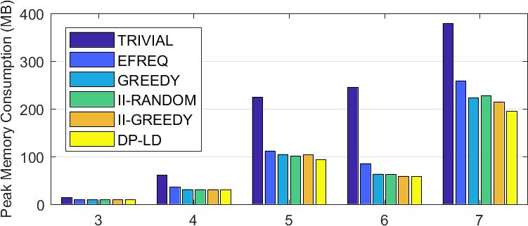
(a)

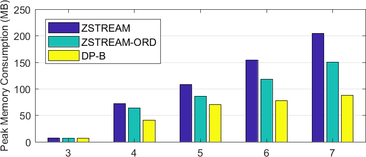
(b)

Figure 9: Memory consumption as a function of the negation pattern size (lower is better): LABEL:sub@fig:memory-order order-based methods; LABEL:sub@fig:memory-tree tree-based methods.

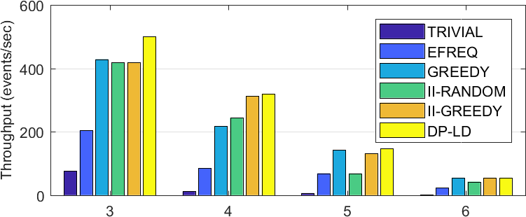
(a)

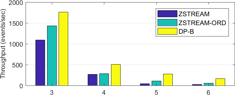
(b)

Figure 10: Throughput as a function of the conjunction pattern size (higher is better): LABEL:sub@fig:throughput-order order-based methods; LABEL:sub@fig:throughput-tree tree-based methods.

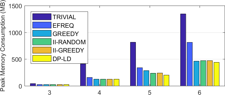
(a)

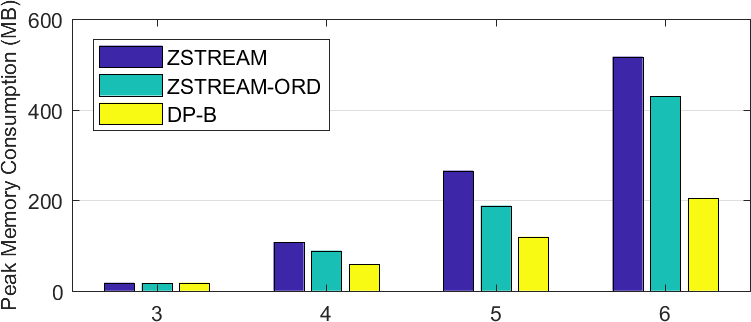
(b)

Figure 11: Memory consumption as a function of the conjunction pattern size (lower is better): LABEL:sub@fig:memory-order order-based methods; LABEL:sub@fig:memory-tree tree-based methods.

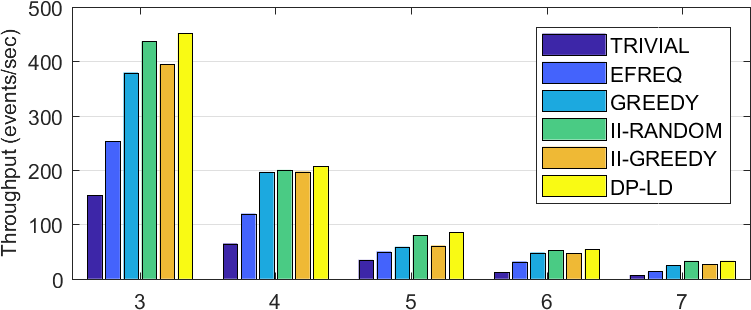
(a)

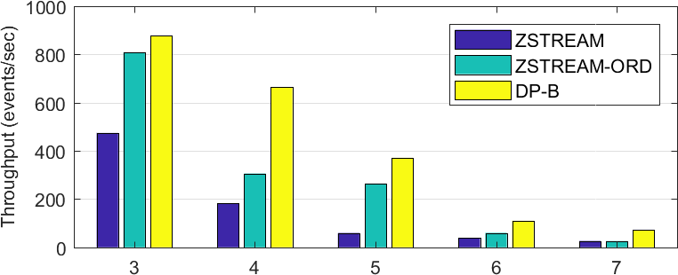
(b)

Figure 12: Throughput as a function of the iteration pattern size (higher is better): LABEL:sub@fig:throughput-order order-based methods; LABEL:sub@fig:throughput-tree tree-based methods.

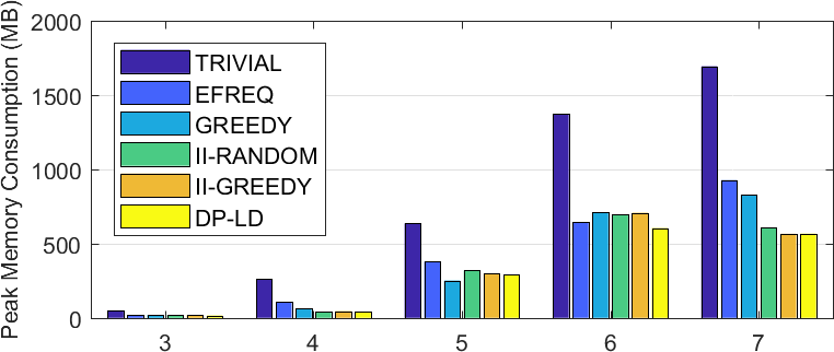
(a)

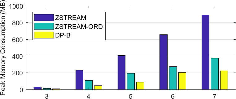
(b)

Figure 13: Memory consumption as a function of the iteration pattern size (lower is better): LABEL:sub@fig:memory-order order-based methods; LABEL:sub@fig:memory-tree tree-based methods.

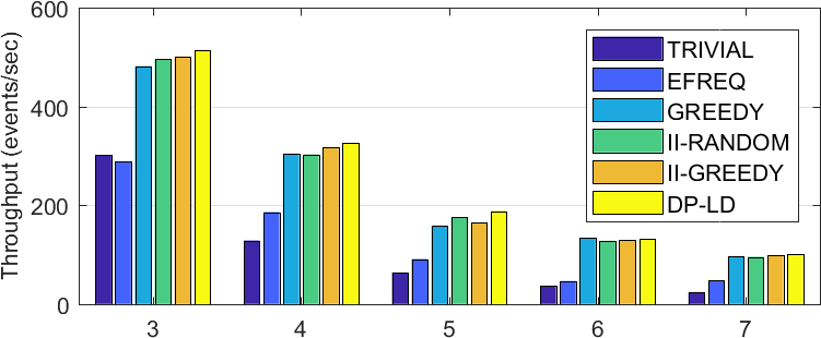
(a)

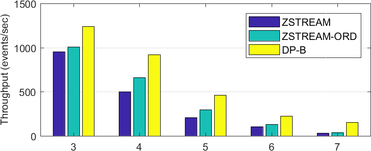
(b)

Figure 14: Throughput as a function of the disjunction pattern size (higher is better): LABEL:sub@fig:throughput-order order-based methods; LABEL:sub@fig:throughput-tree tree-based methods.

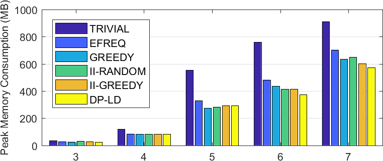
(a)

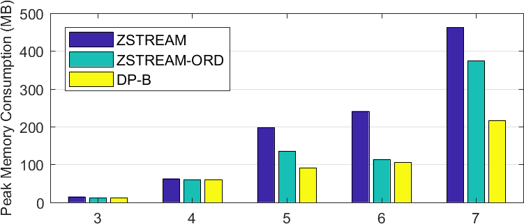
(b)

Figure 15: Memory consumption as a function of the disjunction pattern size (lower is better): LABEL:sub@fig:memory-order order-based methods; LABEL:sub@fig:memory-tree tree-based methods.

In our next experiment, we evaluated the quality of the cost functions used during plan generation. To that end, we created 60 order-based and 60 tree-based plans for patterns of various types using different algorithms. The plans were then executed on the stock dataset. The throughput and the memory consumption measured during each execution are shown in Figure 16 as the function of the cost assigned to each plan by the corresponding function ($Cost_{ord}$ or $Cost_{tree}$). The obtained throughput seems to be inversely proportional to the cost, behaving roughly as $\frac{1}{x^{c}};c\geq 1$. For memory consumption, an approximately linear dependency can be observed. These results match our expectations, as a cheaper plan is supposed to yield better performance and require less memory. We may thus conclude that the costs returned by $Cost_{ord}$ and $Cost_{tree}$ provide a reasonably accurate estimation of the actual performance of a plan.

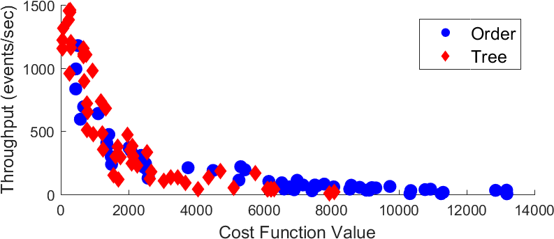
(a)

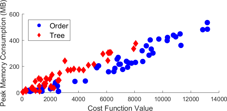
(b)

Figure 16: Performance metrics as a function of the cost computed by the cost functions for order-based and tree-based patterns: LABEL:sub@fig:throughput-cost throughput; LABEL:sub@fig:memory-cost memory consumption.

The above conclusion allowed us to repeat the experiments summarized in Figures 6-15 for larger patterns, using the plan cost as the objective function. We generated 200 patterns of sizes ranging from 3 to 22. We then created a set of plans for each pattern using different algorithms and recorded the resulting plan costs. Due to the exponential growth of the cost with the pattern size, directly comparing the costs was impractical. Instead, the normalized cost was calculated for every plan. The normalized cost of a plan $Pl$ created by an algorithm $A$ for a pattern $P$ was defined as the cost of a plan generated for $P$ by the empirically worst algorithm (the CEP-native EFREQ), divided by the cost of $Pl$.

The results for selected algorithms are depicted in Figure 17LABEL:sub@fig:cost-value. Each data point represents an average normalized cost for all plans of the same size created by the same algorithm. As we observed previously, the DP-based join algorithms consistently produced significantly cheaper plans (up to a factor of 57) than the heuristic alternatives. Also, the worst JQPG method (GREEDY) and the best CPG method (ZSTREAM) produced plans of similar quality, with the former slightly overperforming the latter for larger pattern sizes. The worst-performing EFREQ algorithm was used for normalized cost calculation and is thus not shown in the figure.

Figure 17LABEL:sub@fig:optimization-time presents the plan generation times measured during the above experiment. The results are displayed in logarithmic scale. While all algorithms incur only negligible optimization overhead for small patterns, it grows rapidly for methods based on dynamic programming (for a pattern of length 22, it took over 50 hours to create a plan using DP-B). This severely limits the applicability of the DP-based approaches when the number of events in a pattern is high. On the other hand, all non-dynamic algorithms were able to complete in under a second even for the largest tested patterns. The join-based greedy algorithm (GREEDY) demonstrated the best overall trade-off between optimization time and quality.

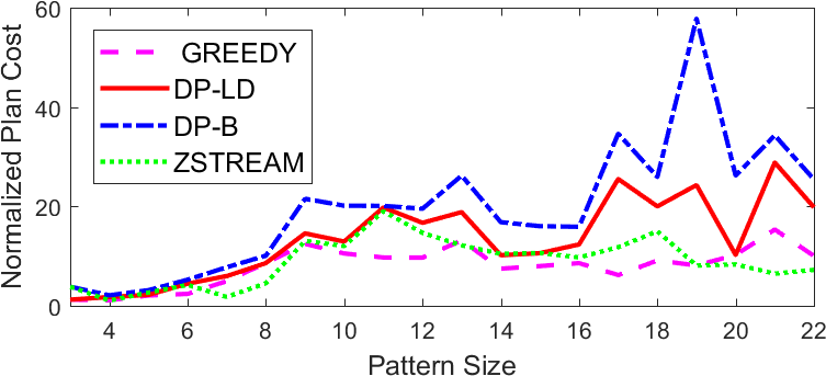
(a)

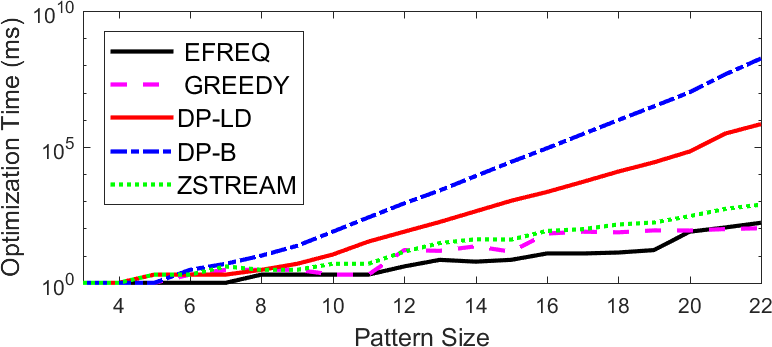
(b)

Figure 17: Generation of large plans (selected algorithms): LABEL:sub@fig:cost-value average normalized plan cost (higher is better); LABEL:sub@fig:optimization-time average plan generation time (logarithmic scale, lower is better). The results are presented as a function of pattern size.

Next, we studied the performance of the hybrid throughput-latency cost model introduced in Section 6.1. Each of the 6 JQPG-based methods discussed in Section 7.1 was evaluated using three different values for the throughput-latency trade-off parameter $\alpha$: 0, 0.5 and 1. Note that for the first case ($\alpha=0$) the resulting cost model is identical to the one defined in Section 4 and used in the experiments above. For each algorithm and for each value of $\alpha$, the throughput and the average latency (in milliseconds) were measured.

Figure 18 demonstrates the results, averaged over 500 patterns included in the sequence pattern set. Measurements obtained using the same algorithm are connected by straight lines, and the labels near the highest points (diamonds) indicate the algorithms corresponding to these points. It can be seen that increasing the value of $\alpha$ results in a significantly lower latency. However, this also results in a considerable drop in throughput for most algorithms. By fine-tuning this parameter, the desired latency can be achieved with minimal loss in throughput. It can also be observed that the tree-based algorithms DP-B and ZSTREAM-ORD (and, to some extent, the order-based II-GREEDY) achieve a substantially better throughput-latency trade-off as compared to other methods.

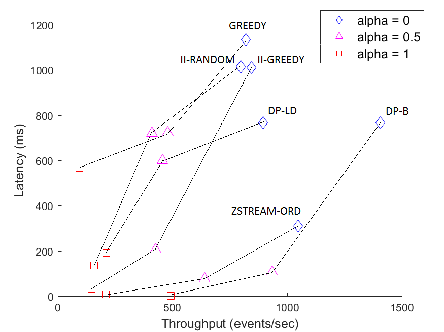
Figure 18: Throughput vs. latency using different values for the alpha parameter of the cost model.

Finally, we performed a comparative throughput evaluation of the sequence pattern set under three different event selection strategies: skip-till-any-match, skip-till-next-match and contiguity (Section 6.2). The results are depicted in Figure 19 for all algorithms under examination. Due to large performance gaps between the examined methods, the results are displayed in logarithmic scale.

For skip-till-next-match, JQPG methods hold a clear advantage, albeit less significant than the one demonstrated above for skip-till-any-match. The opposite observation can be made about the contiguity strategy, where the trivial algorithm following a static plan outperforms other, more complicated methods. Due to the simplicity of the event detection process and the lack of nondeterminism in this case, the plan set by an input specification always performs best, while the alternatives introduce a slight additional overhead of reordering and event buffering.

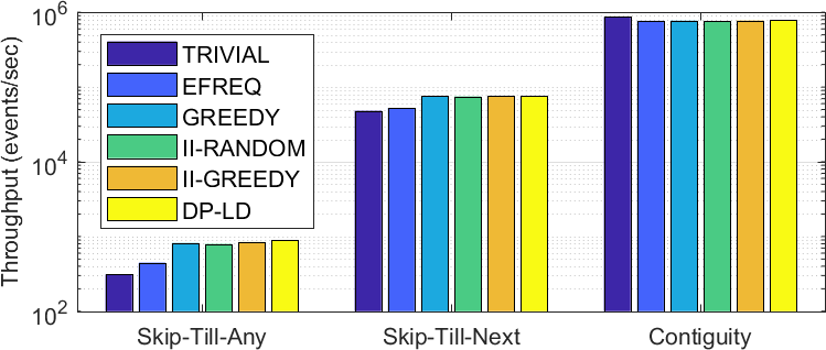
(a)

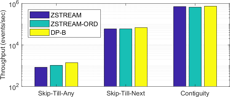
(b)

Figure 19: Throughput for different event selection strategies (logarithmic scale): LABEL:sub@fig:strategy-order order-based methods; LABEL:sub@fig:strategy-tree tree-based methods.

8 Related Work

Systems for scalable extraction of complex events from high-speed information flows have become an increasingly important research field during last decades, as a result of the rising demand for technologies of this type [16, 21]. Their inception can be traced to earlier systems for massive data stream processing, such as TelegraphCQ [11], NiagaraCQ [12], Aurora/Borealis [3] and Stream [8]. Later, a broad variety of general purpose complex event processing solutions emerged [4, 6, 10, 15, 18, 29, 33, 35, 41, 44, 50], including the widely used commercial CEP providers, such as Esper [2] and IBM System S [7].

Various performance optimization techniques are implemented in complex event processing systems [23]. In [41], a rewriting framework is described, based on unifying and splitting patterns. A method for efficient Kleene closure evaluation based on sharing with postponed operators is discussed in [52], while in [40] the authors solve the above problem by maintaining a compact graph encoding of event sequences and utilizing it for effective reuse. RunSAT [20] utilizes another approach, preprocessing a pattern and setting optimal points for termination of the detection process. ZStream [35] presents an optimization framework for optimal tree generation, based on a complex cost model. As already shown above, since the leaves of an evaluation tree cannot be reordered, it only searches through a partial solution space. Advanced methods were also proposed for multi-query CEP optimization [17, 34, 42, 43, 53].

CEP engines utilizing the order-based evaluation approach have also adopted different optimization strategies. SASE [50], Cayuga [18] and T-Rex [15] design efficient data structures to enable smart runtime memory management. These NFA-based mechanisms do not support out-of-order processing, and hence are still vulnerable to the problem of large intermediate results. In [6, 29, 44], various pattern reordering methods for efficient order-based complex event detection are described. None of these works takes the selectivities of the event constraints into account.

Estimating an optimal evaluation plan for a join query has long been considered one of the most important problems in the area of query optimization [46]. Multiple authors have shown the NP-completeness of this problem for arbitrary query graphs [13, 24], and a wide range of methods were proposed to provide either exact or approximate close-to-optimal solutions [30, 31, 32, 36, 45, 46, 47].

Methods for join query plan generation can be roughly divided into two main categories. The heuristic algorithms, as their name suggests, utilize some kind of heuristic function or approach to perform efficient search through the huge solution space. They are often applied in conjunction with combinatorial [26, 46, 47] or graph-based [31, 32] techniques. The heuristic algorithms produce fast solutions, but the resulting execution plans are often far from the optimum.

The second category of JQPG algorithms, the exhaustive search algorithms, provide provable guarantees on the optimality of the returned solutions. These methods are often based on dynamic programming [36, 45] and thus suffer from worst-case exponential complexity. To solve this issue, hybrid techniques were proposed, making it possible to set the trade-off between the speed of heuristic approaches and the precision of DP-based approaches [30].

Incorporating join optimization techniques from traditional DBMSs was already considered in the related fields, such as XPath [22] and data stream processing [12]. For the best of our knowledge, our work is the first to address the CEP-specific challenges and to provide a formal reduction.

9 Conclusions and Future Work

In this paper, we studied the relationship between two important and relevant problems, CEP Plan Generation and Join Query Plan Generation. It was shown that the CPG problem is equivalent to JQPG for a subset of pattern types, and reducible to it for other types. We discussed how close-to-optimal solutions to CPG can be efficiently obtained by applying existing JQPG methods. CEP-related challenges, such as detection latency and event selection strategies, were addressed. The presented experimental study supported our analysis by demonstrating how the evaluation plans created by some of the well-known join algorithms outperform those produced by the methods traditionally used in CEP systems.

Utilizing join-related techniques in the field of CEP introduces additional, not yet addressed challenges, such as efficient tracking of real-time predicate selectivities and handling inter-predicate dependencies. We intend to target these challenges in our future research, in addition to the directions outlined throughout the paper.

Appendix A ASI Property of the Order-Based Cost Functions

In this appendix, we will formally prove that the order-based CPG cost functions $Cost_{ord}^{trpt}$ and $Cost_{ord}^{lat}$ presented in Sections 4.1 and 6.1 respectively have the adjacent sequence interchange (ASI) property, defined in [37]. As we discussed in Section 4.3, polynomial-time algorithms were developed for join ordering of acyclic queries subject to cost functions that have this property [24, 31]. Since all JQPG algorithms demonstrated in this paper are executed subject to the left-deep tree cost function $Cost_{LDJ}$, we do not use this result directly for solving the CPG problem. However, the throughput- and latency-related functions can potentially be employed directly for solving the join ordering problem in streaming database systems, and hence it is important to show their ASI property as a part of our work.

We will start with the definition of the ASI property.

Definition 1

A cost function $C$ has the adjacent sequence interchange (ASI) property, if and only if there exists a rank function $rank\left(s\right)$ for sequences $s$, such that for all sequences $a,b$ and for all non-empty sequences $v,u$ the following holds:

$$C\left(auvb\right)\leq C\left(avub\right)\Leftrightarrow rank\left(u\right)\leq rank\left(v\right).$$

We will first provide the proof for the throughput-related cost function $Cost_{ord}^{trpt}$ . To that end, we will utilize the idea from a similar proof in [13].

Theorem 5

The cost function $Cost_{ord}^{trpt}$ has the ASI property.

Let $P$ be a pure conjunctive pattern over the event types $T_{1},\cdots,T_{n}$ with an acyclic query graph. Recall that the cost function is defined as follows:

$$Cost_{ord}^{trpt}\left(O\right)=\sum_{k=1}^{n}\left(W^{k}\cdot\prod_{i=1}^{k}r_{p_{i}}\cdot\prod_{i,j\leq k;i\leq j}sel_{p_{i},p_{j}}\right),$$

where $O=\left(T_{p_{1}},T_{p_{2}},\cdots T_{p_{n}}\right);p_{i}\in[1,n]$.

Due to the acyclicity of the pattern, each event type $T_{p_{i}}$ will only have one predicate with the event types preceding it in $O$. Further, if we set the root of the query tree at some event type $T_{R}$, this predicate can be uniquely determined for any other type, as follows from the uniqueness of a path between two nodes in a tree. For each $T_{i}\neq T_{R}$, we will denote this predicate as $c_{i}^{R}$, and its selectivity will be thus denoted as $sel_{i}^{R}$. For the root event type, we set $sel_{R}^{R}=1$. Rewriting the cost function definition accordingly, we get:

$$Cost_{ord}^{trpt}\left(O\right)=\sum_{k=1}^{n}\prod_{i=1}^{k}\left(W\cdot r_{p_{i}}\cdot sel_{i}^{R}\right).$$

We will now define the following auxiliary functions, defined on any sequence $s$ of size $m$, consisting of events $T_{1},\cdots,T_{n}$:

$$C\left(s\right)=\sum_{k=1}^{m}\prod_{i=1}^{k}\left(W\cdot r_{p_{i}}\cdot sel_{i}^{R}\right);\>C\left(\varepsilon\right)=0$$

$$T\left(s\right)=\prod_{i=1}^{m}\left(W\cdot r_{p_{i}}\cdot sel_{i}^{R}\right);\>T\left(\varepsilon\right)=1.$$

Note that the above functions only depend on the selection of the root $R$.

It can be observed that $C\left(O\right)=Cost_{ord}^{trpt}\left(O\right)$ for any evaluation order $O$. In addition, the following holds:

$$C\left(s_{1}s_{2}\right)=C\left(s_{1}\right)+T\left(s_{1}\right)\cdot C\left(s_{2}\right).$$

We will now define the rank function as follows:

$$rank\left(s\right)=\frac{T\left(s\right)-1}{C\left(s\right)}$$

We will demonstrate the ASI property for the rank function $rank$. Let $a,b$ arbitrary sequences and $v,u$ arbitrary non-empty sequences. Then:

$$C\left(auvb\right) \leq C\left(avub\right)\Leftrightarrow$$

$$C\left(a\right)+T\left(a\right)\cdot C\left(uvb\right) \leq C\left(a\right)+T\left(a\right)\cdot C\left(vub\right)\Leftrightarrow$$

$$C\left(u\right)+T\left(u\right)\cdot C\left(vb\right) \leq C\left(v\right)+T\left(v\right)\cdot C\left(ub\right)\Leftrightarrow$$

$$C\left(u\right)+T\left(u\right)\cdot\left(C\left(v\right)+T\left(v\right)\cdot C\left(b\right)\right) \leq C\left(v\right)+T\left(v\right)\cdot\left(C\left(u\right)+T\left(u\right)\cdot C\left(vb\right)\right)\Leftrightarrow$$

$$C\left(u\right)+T\left(u\right)\cdot C\left(v\right)+T\left(u\right)\cdot T\left(v\right)\cdot C\left(b\right) \leq C\left(v\right)+T\left(v\right)\cdot C\left(u\right)+T\left(v\right)\cdot T\left(u\right)\cdot C\left(b\right)\Leftrightarrow$$

$$T\left(u\right)\cdot C\left(v\right)-C\left(v\right) \leq T\left(v\right)\cdot C\left(u\right)-C\left(u\right)\Leftrightarrow$$

$$\frac{T\left(u\right)-1}{C\left(u\right)} \leq\frac{T\left(v\right)-1}{C\left(v\right)}\Leftrightarrow$$

$$rank\left(u\right) \leq rank\left(v\right).$$

The above transitions are possible due to the positivity of $T\left(s\right)$ and the positivity of $C\left(s\right)$ for non-empty sequences.$\blacksquare$

We will now proceed to the latency-related cost function $Cost_{ord}^{lat}$ .

Theorem 6

The cost function $Cost_{ord}^{lat}$ has the ASI property.

Let $P$ be a pure conjunctive pattern over the event types $T_{1},\cdots,T_{n}$ with an acyclic query graph. Recall that the cost function is defined as follows:

$$Cost_{ord}^{lat}\left(O\right)=\sum_{T_{i}\in Succ_{O}\left(T_{n}\right)}W\cdot r_{i},$$

where $O=\left(T_{p_{1}},T_{p_{2}},\cdots T_{p_{n}}\right);p_{i}\in[1,n]$, $T_{n}$ is the last event type in the order induced by the pattern, and $Succ_{O}\left(T_{n}\right)$ denotes the event types succeeding $T_{n}$ in $O$.

For each sequence $s$ over the above types, we will define the following function accepting an event type $T_{i}$ as a parameter:

$$g_{s}\left(T_{i}\right)=\begin{cases}W\cdot r_{i}&if\>T_{i}\in Succ_{s}\left(T_{n}\right)\\ 0&otherwise.\end{cases}$$

$Cost_{ord}^{lat}$ can be now rewritten in the following form:

$$Cost_{ord}^{lat}\left(O\right)=\sum_{i=1}^{n}g_{O}\left(T_{i}\right).$$

The rank function will be defined as follows:

$$rank\left(s\right)=\begin{cases}\sum_{T_{i}\in s}g_{s}\left(T_{i}\right)&if\>T_{n}\in s\\ 0&otherwise.\end{cases}$$

We will now demonstrate the ASI property of $Cost_{ord}^{lat}$ by examining the following cases for non-empty sequences $u,v$:

1. $T_{n}\notin u$ and $T_{n}\notin v$: in this case, $rank\left(u\right)=rank\left(v\right)=0$. Examine the expressions $Cost_{ord}^{lat}\left(auvb\right)$ and $Cost_{ord}^{lat}\left(avub\right)$ for some sequences $a,b$. If $T_{n}\notin a$, then obviously $u$ and $v$ do not contribute any event type with a non-zero value of $g_{auvb}\left(T_{i}\right)$ (or $g_{avub}\left(T_{i}\right)$, symmetrically), hence $Cost_{ord}^{lat}\left(auvb\right)=Cost_{ord}^{lat}\left(avub\right)=Cost_{ord}^{lat}\left(ab\right)$. Otherwise, since $u,v,b\subseteq Succ_{auvb}\left(T_{n}\right)$, the cost function for $u,v,b$ is commutative by definition and thus $Cost_{ord}^{lat}\left(auvb\right)=Cost_{ord}^{lat}\left(avub\right)$.

2. $T_{n}\in v$: in this case, we have $rank\left(v\right)\geq 0$ by non-negativity of $g_{s}$ and $rank\left(u\right)=0$ since $u$ and $v$ must be disjoint. Consequently, $rank\left(u\right)\leq rank\left(v\right)$. Now, examine the first cost expression:

   $$Cost_{ord}^{lat}\left(auvb\right)=\sum_{T_{i}\in auvb}g_{auvb}\left(T_{i}\right)=$$

   $$=\sum_{T_{i}\in a}g_{auvb}\left(T_{i}\right)+\sum_{T_{i}\in u}g_{auvb}\left(T_{i}\right)+\sum_{T_{i}\in v}g_{auvb}\left(T_{i}\right)+\sum_{T_{i}\in b}g_{auvb}\left(T_{i}\right)=$$

   $$=0+0+rank\left(v\right)+\sum_{T_{i}\in b}\left(W\cdot r_{i}\right).$$

   For the second cost expression, we obtain the following:

   $$Cost_{ord}^{lat}\left(avub\right)=\sum_{T_{i}\in avub}g_{avub}\left(T_{i}\right)=$$

   $$=\sum_{T_{i}\in a}g_{avub}\left(T_{i}\right)+\sum_{T_{i}\in v}g_{avub}\left(T_{i}\right)+\sum_{T_{i}\in u}g_{avub}\left(T_{i}\right)+\sum_{T_{i}\in b}g_{avub}\left(T_{i}\right)=$$

   $$=0+rank\left(v\right)+\sum_{T_{i}\in u}\left(W\cdot r_{i}\right)+\sum_{T_{i}\in b}\left(W\cdot r_{i}\right).$$

   The difference between these expressions is:

   $$Cost_{ord}^{lat}\left(avub\right)-Cost_{ord}^{lat}\left(auvb\right)=\sum_{T_{i}\in u}\left(W\cdot r_{i}\right).$$

   By non-negativity of time windows and arrival rates, we thus get $Cost_{ord}^{lat}\left(auvb\right)\leq Cost_{ord}^{lat}\left(avub\right)$.

3. $T_{n}\in u$: this case is symmetrical to case 2, and identical steps are applied to show that $rank\left(v\right)\leq rank\left(u\right)$ and $Cost_{ord}^{lat}\left(avub\right)\leq Cost_{ord}^{lat}\left(auvb\right)$.

To summarize, we have demonstrated that in all cases the condition of the ASI property holds, which completes the proof.$\blacksquare$

References

- [1] http://www.eoddata.com.
- [2] http://www.espertech.com.
- [3] D. J. Abadi, Y. Ahmad, M. Balazinska, M. Cherniack, J. Hwang, W. Lindner, A. S. Maskey, E. Rasin, E. Ryvkina, N. Tatbul, Y. Xing, and S. Zdonik. The design of the borealis stream processing engine. In CIDR, pages 277–289, 2005.
- [4] A. Adi and O. Etzion. Amit - the situation manager. The VLDB Journal, 13(2):177–203, 2004.
- [5] J. Agrawal, Y. Diao, D. Gyllstrom, and N. Immerman. Efficient pattern matching over event streams. In SIGMOD, pages 147–160, 2006.
- [6] M. Akdere, U. Çetintemel, and N. Tatbul. Plan-based complex event detection across distributed sources. Proc. VLDB Endow., 1(1):66–77, 2008.
- [7] L. Amini, H. Andrade, R. Bhagwan, F. Eskesen, R. King, P. Selo, Y. Park, and C. Venkatramani. Spc: A distributed, scalable platform for data mining. In Proceedings of the 4th International Workshop on Data Mining Standards, Services and Platforms, pages 27–37, New York, NY, USA, 2006. ACM.
- [8] A. Arasu, B. Babcock, S. Babu, J. Cieslewicz, M. Datar, K. Ito, R. Motwani, U. Srivastava, and J. Widom. STREAM: The Stanford Data Stream Management System, pages 317–336. Springer Berlin Heidelberg, Berlin, Heidelberg, 2016.
- [9] S. Babu, R. Motwani, K. Munagala, I. Nishizawa, and J. Widom. Adaptive ordering of pipelined stream filters. In Proceedings of the 2004 ACM SIGMOD International Conference on Management of Data, pages 407–418, New York, NY, USA, 2004. ACM.
- [10] R. S. Barga, J. Goldstein, M. H. Ali, and M. Hong. Consistent streaming through time: A vision for event stream processing. In CIDR, pages 363–374, 2007.
- [11] S. Chandrasekaran, O. Cooper, A. Deshpande, M. J. Franklin, J. M. Hellerstein, W. Hong, S. Krishnamurthy, S. Madden, V. Raman, F. Reiss, and M. A. Shah. Telegraphcq: Continuous dataflow processing for an uncertain world. In CIDR, 2003.
- [12] J. Chen, D. J. DeWitt, F. Tian, and Y. Wang. Niagaracq: A scalable continuous query system for internet databases. SIGMOD Rec., 29(2):379–390, 2000.
- [13] S. Cluet and G. Moerkotte. On the complexity of generating optimal left-deep processing trees with cross products. In Proceedings of the 5th International Conference on Database Theory, ICDT ’95, pages 54–67, London, UK, 1995. Springer-Verlag.
- [14] G. Cugola and A. Margara. Tesla: a formally defined event specification language. In DEBS, pages 50–61. ACM, 2010.
- [15] G. Cugola and A. Margara. Complex event processing with t-rex. J. Syst. Softw., 85(8):1709–1728, 2012.
- [16] G. Cugola and A. Margara. Processing flows of information: From data stream to complex event processing. ACM Comput. Surv., 44(3):15:1–15:62, 2012.
- [17] A. Demers, J. Gehrke, M. Hong, M. Riedewald, and W. White. Towards expressive publish/subscribe systems. In Proceedings of the 10th International Conference on Advances in Database Technology, pages 627–644. Springer-Verlag.
- [18] A. Demers, J. Gehrke, B. Panda, M. Riedewald, V. Sharma, and W. White. Cayuga: A general purpose event monitoring system. In CIDR, pages 412–422, 2007.
- [19] A. Deshpande, Z. Ives, and V. Raman. Adaptive query processing. Found. Trends databases, 1(1):1–140, January 2007.
- [20] L. Ding, S. Chen, E. A. Rundensteiner, J. Tatemura, W. P. Hsiung, and K. S. Candan. Runtime semantic query optimization for event stream processing. IEEE 24th International Conference on Data Engineering (ICDE), 0:676–685, 2008.
- [21] O. Etzion and P. Niblett. Event Processing in Action. Manning Publications Co., 2010.
- [22] T. Grust, J. Rittinger, and J. Teubner. Why off-the-shelf rdbmss are better at xpath than you might expect. In Proceedings of the 2007 ACM SIGMOD International Conference on Management of Data, SIGMOD ’07, pages 949–958, New York, NY, USA, 2007. ACM.
- [23] M. Hirzel, R. Soulé, S. Schneider, B. Gedik, and R. Grimm. A catalog of stream processing optimizations. ACM Comput. Surv., 46(4):46:1–46:34, March 2014.
- [24] T. Ibaraki and T. Kameda. On the optimal nesting order for computing n-relational joins. ACM Trans. Database Syst., 9(3):482–502, 1984.
- [25] Y. Ioannidis and Y. Kang. Left-deep vs. bushy trees: An analysis of strategy spaces and its implications for query optimization. SIGMOD Rec., 20(2):168–177, April 1991.
- [26] Y. E. Ioannidis and Y. Kang. Randomized algorithms for optimizing large join queries. SIGMOD Rec., 19(2):312–321, May 1990.
- [27] I. Kolchinsky and A. Schuster. Efficient adaptive detection of complex event patterns. CoRR, abs/1801.08588, 2017.
- [28] I. Kolchinsky, A. Schuster, and D. Keren. Efficient detection of complex event patterns using lazy chain automata. CoRR, abs/1612.05110, 2016.
- [29] I. Kolchinsky, I. Sharfman, and A. Schuster. Lazy evaluation methods for detecting complex events. In DEBS, pages 34–45. ACM, 2015.
- [30] D. Kossmann and K. Stocker. Iterative dynamic programming: A new class of query optimization algorithms. ACM Trans. Database Syst., 25(1):43–82, 2000.
- [31] R. Krishnamurthy, H. Boral, and C. Zaniolo. Optimization of nonrecursive queries. In Proceedings of the 12th International Conference on Very Large Data Bases, VLDB ’86, pages 128–137, San Francisco, CA, USA, 1986. Morgan Kaufmann Publishers Inc.
- [32] C. Lee, C.S. Shih, and Y.H. Chen. A graph-theoretic model for optimizing large join queries. In DASFAA, volume 6 of Advanced Database Research and Development Series, pages 87–96. World Scientific, 1997.
- [33] M. Liu, E. Rundensteiner, D. Dougherty, C. Gupta, S. Wang, I. Ari, and A. Mehta. High-performance nested CEP query processing over event streams. In Proceedings of the 27th International Conference on Data Engineering, ICDE 2011, pages 123–134.
- [34] M. Liu, E. Rundensteiner, K. Greenfield, C. Gupta, S. Wang, I. Ari, and A. Mehta. E-cube: Multi-dimensional event sequence analysis using hierarchical pattern query sharing. In Proceedings of the 2011 ACM SIGMOD International Conference on Management of Data, SIGMOD ’11, pages 889–900, New York, NY, USA, 2011. ACM.
- [35] Y. Mei and S. Madden. Zstream: a cost-based query processor for adaptively detecting composite events. In SIGMOD Conference, pages 193–206. ACM, 2009.
- [36] G. Moerkotte and T. Neumann. Analysis of two existing and one new dynamic programming algorithm for the generation of optimal bushy join trees without cross products. In Proceedings of the 32nd International Conference on Very Large Data Bases, pages 930–941. VLDB Endowment, 2006.
- [37] C. Monma and J. Sidney. Sequencing with series-parallel precedence constraints. Math. Oper. Res., 4(3):215–224, August 1979.
- [38] K. Ono and G. Lohman. Measuring the complexity of join enumeration in query optimization. In Proceedings of the 16th International Conference on Very Large Data Bases, VLDB ’90, pages 314–325, San Francisco, CA, USA, 1990. Morgan Kaufmann Publishers Inc.
- [39] M. Orlowski. On Optimization Of Joins In Distributed Database System, pages 106–114.
- [40] O. Poppe, C. Lei, S. Ahmed, and E. Rundensteiner. Complete event trend detection in high-rate event streams. In Proceedings of the 2017 ACM International Conference on Management of Data, SIGMOD ’17, pages 109–124, New York, NY, USA, 2017. ACM.
- [41] E. Rabinovich, O. Etzion, and A. Gal. Pattern rewriting framework for event processing optimization. In Proceedings of the 5th ACM International Conference on Distributed Event-based Systems, pages 101–112. ACM, 2011.
- [42] M. Ray, C. Lei, and E. A. Rundensteiner. Scalable pattern sharing on event streams. In Proceedings of the 2016 International Conference on Management of Data, SIGMOD ’16, pages 495–510, New York, NY, USA, 2016. ACM.
- [43] M. Ray, E. Rundensteiner, M. Liu, C. Gupta, S. Wang, and I. Ari. High-performance complex event processing using continuous sliding views. In Proceedings of the 16th International Conference on Extending Database Technology, EDBT ’13, pages 525–536, New York, NY, USA, 2013. ACM.
- [44] N. P. Schultz-Møller, M. M., and P. R. Pietzuch. Distributed complex event processing with query rewriting. In DEBS. ACM, 2009.
- [45] P. Selinger, M. Astrahan, D. Chamberlin, R. Lorie, and T. Price. Access path selection in a relational database management system. In Proceedings of the 1979 ACM SIGMOD Conference, pages 23–34, 1979.
- [46] M. Steinbrunn, G. Moerkotte, and A. Kemper. Heuristic and randomized optimization for the join ordering problem. VLDB J., 6(3):191–208, 1997.
- [47] A. Swami. Optimization of large join queries: Combining heuristics and combinatorial techniques. SIGMOD Rec., 18(2):367–376, 1989.
- [48] I. Trummer and C. Koch. Multi-objective parametric query optimization. SIGMOD Rec., 45(1):24–31, 2016.
- [49] B. Vance and D. Maier. Rapid bushy join-order optimization with cartesian products. SIGMOD Rec., 25(2):35–46, June 1996.
- [50] E. Wu, Y. Diao, and S. Rizvi. High-performance complex event processing over streams. In SIGMOD Conference, pages 407–418. ACM, 2006.
- [51] I. Yi, J. G. Lee, and K. Y. Whang. Apam: Adaptive eager-lazy hybrid evaluation of event patterns for low latency. In Proceedings of the 25th ACM Conference on Information and Knowledge Management, pages 2275–2280. ACM, 2016.
- [52] H. Zhang, Y. Diao, and N. Immerman. On complexity and optimization of expensive queries in complex event processing. In SIGMOD, pages 217–228, 2014.
- [53] S. Zhang, H. T. Vo, D. Dahlmeier, and B. He. Multi-query optimization for complex event processing in SAP ESP. In 33rd IEEE International Conference on Data Engineering, ICDE 2017, San Diego, CA, USA, April 19-22, 2017, pages 1213–1224, 2017.