Curvature calculations for antitrees

Abstract

In this article we prove that antitrees with suitable growth properties are examples of infinite graphs exhibiting strictly positive curvature in various contexts: in the normalized and non-normalized Bakry-Émery setting as well in the Ollivier-Ricci curvature case. We also show that these graphs do not have global positive lower curvature bounds, which one would expect in view of discrete analogues of the Bonnet-Myers theorem. The proofs in the different settings require different techniques.

1 Introduction and results

The main protagonists in this article are antitrees. While these examples had been studied already in 1988, they were given the name antitree in talks by Radoslaw Wojciechowsi around 2010. A proper definition of antitrees, in their most general form, appeared first in [19]. Like in the case of a tree, the vertices of an antitree are partitioned in generations $V_{i}$ with the first generation $V_{1}$ called its root set. While trees are connected graphs with as few connections as possible between subsequent generations, antitees have the maximal number of connections. More precisely, antritrees are simple (i.e., no loops and no multiple edges), connected graphs such that

• any root vertex $x\in V_{1}$ is connected to all vertices in $V_{2}$, and no vertices in $V_{k}$, $k\geq 3$,

• any vertex $x\in V_{k}$, $k\geq 2$, is connected to all vertices in $V_{k-1}$ and $V_{k+1}$, and no vertices in $V_{l}$, $|k-l|\geq 2$.

Note that this definition allows for the possibility of edges between vertices of the same generation. We will refer to such edges as spherical edges. Edges between vertices of different generations are called radial edges. Any radial or spherical edge incident to a vertex in $V_{1}$ is called radial or spherical root-edge, respectively. All other edges are called inner edges.

Antitrees are particularly interesting examples with regards to stochastic completeness. Section 2, provided by Radoslaw Wojciechowki, gives a more in-depth look at the history of antitrees. In this article, we investigate curvature properties of antitrees. Relations between curvature asymptotics and stochastic completeness were investigated recently in [17] in the Bakry-Émery setting and in [22] in the Ollivier-Ricci curvature setting.

For our curvature considerations, we consider only antitrees where the induced subgraph of any one generation $V_{k}$ is complete, i.e., any two vertices in the same generation are neighbours. For any given finite or infinite sequence $(a_{k})_{1\leq k\leq N}$, $N\in{\mathbb{N}}\cup\{\infty\}$, the corresponding unique such antitree with $|V_{k}|=a_{k}$ for all $1\leq k\leq N$ is denoted by ${\mathcal{AT}}((a_{k}))$. Note that in the case of a finite antitree, that is $N<\infty$, (ii) has to be understood in the case $k=N$ that any vertex $x\in V_{N}$ is connectd to all vertices in $V_{N-1}$. Later in this introduction, we will only present results for infinite antitrees but, since curvature is a local notion, we need only investigate curvatures of suitable finite antitrees for the proofs.

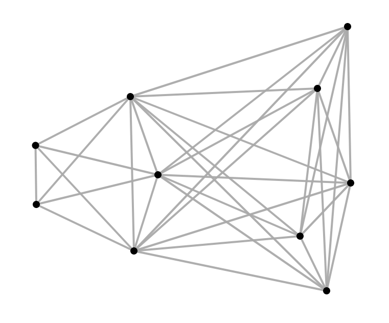
Figure 1: The antitree $\mathcal{AT}((2,3,5))$

Two particular curvature notions on graphs have been studied actively in recent years:

• Bakry-Émery curvature taking values on the vertices and based on Bochner’s formula with respect to a suitable graph Laplacian,

• Ollivier-Ricci curvature taking values on the edges and based on optimal transport of lazy random walks.

Basic graph theoretical notions are introduced in Section 3.1 and precise definitions of these curvature concepts are given in Sections 3.2 and 3.3, respectively.

For both curvature notions there are graph theoretical analogues of the fundamental Bonnet-Myers Theorem for Riemannian manifolds with strictly positive Ricci curvature bounded away from zero.

Let us first consider Bakry-Émery curvature. Generally, on a combinatorial graph $G=(V,E)$ with vertex set $V$ and edge set $E$, the graph Laplacian on functions $f:V\to{\mathbb{R}}$ is of the form

$$\Delta f(x)=\frac{1}{\mu(x)}\sum_{y\sim x}(f(y)-f(x)),$$ (1.1)

with a vertex measure $\mu:V\to(0,\infty)$. In this article, we consider two specific choices of vertex measures:

• $\mu\equiv 1$, which we refer to as the non-normalized case,

• $\mu(x)=d_{x}$ (the vertex degree of $x\in V$), which we refer to as the normalized case.

The corresponding discrete Bonnet-Myers theorems in both settings are as follows:

Theorem 1.1 (see [21]).

Let $G=(V,E)$ be a connected graph satisfying $CD(K,\infty)$ for some $K>0$ in the non-normalized case and $d_{x}\leq D$ for all $x\in V$ and some finite $D$. Then $G$ is a finite graph and, furthermore,

$${\rm{diam}}(G)\leq\frac{2D}{K}.$$

Theorem 1.2 (see [21]).

Let $G=(V,E)$ be a connected graph satisfying $CD(K,\infty)$ for some $K>0$ in the normalized case (possibly of unbounded vertex degree). Then $G$ is a finite graph and, furthermore,

$${\rm{diam}}(G)\leq\frac{2}{K}.$$

Ollivier-Ricci curvature depends upon an idleness parameter $p\in[0,1]$ describing the laziness of the associated random walk. Here, the discrete Bonnet-Myers theorem takes the following form:

Theorem 1.3 (see [23]).

Let $G=(V,E)$ be a connected graph satisfying $\kappa_{p}(x,y)\geq K>0$ for all $x\sim y$ and a fixed idleness $p\in[0,1]$. Then $G$ is a finite graph and, furthermore,

$${\rm{diam}}(G)\leq\frac{2(1-p)}{K}.$$ (1.2)

These results give rise to the following natural questions:

• Do there exist examples of infinite connected graphs with strictly positive curvature? (That is, relaxing the condition of a uniform strictly positive lower curvature bound.)

• In the non-normalized case, doe there exist an infinite connected graphs satisfying $CD(K,\infty)$ for $K>0$ of unbounded vertex degree?

This paper provides a positive answer to the first question. In fact, we show that antitrees ${\mathcal{AT}}((a_{k}))$ with suitable growth properties of the infinite sequence $(a_{k})$ have strictly positive curvature for all curvature notions mentioned above. More precisely, we have the following in the Bakry-Émery curvature case:

Theorem 1.4.

In both the normalized and non-normalized setting, the infinite antitree ${\mathcal{AT}}((k))$ satisfies $CD(K_{x},\infty,x)$ for all vertices $x$ with a family of constants $K_{x}>0$ depending only on the generation of $x$. Furthermore,

$$\liminf_{k\to\infty,\,x\in V_{k}}K_{x}=0.$$

Remark 1.5.

In fact, the method of proof relies on some Maple calculations which can be extended to also provide the following results (without going into the details):

• Linear growth: The same curvature results hold true for the infinite antitrees
  ${\mathcal{AT}}((1+(k-1)t))$ with arbitrary $t\in{\mathbb{N}}$.

• Exponential growth: The same curvature results hold true for the infinite antitree ${\mathcal{AT}}((2^{k-1}))$ in the normalized case and fails to satisfy $CD(0,\infty)$ in the non-normalized case.

Due to Bakry-Émery curvature being a local property, in order to calculate the curvatures ${\mathcal{K}}_{G,x}(\infty)$ of vertices $x$ in the first two generations of $G={\mathcal{AT}}((2^{k-1}))$ as defined later in (3.1), it is sufficient to consider the graph presented in Figures 3 and 3 (spherical edges of $2$-spheres around a vertex do not contribute to the curvature, see [7]). These figures are in agreement with the statements in Remark 1.5(ii).

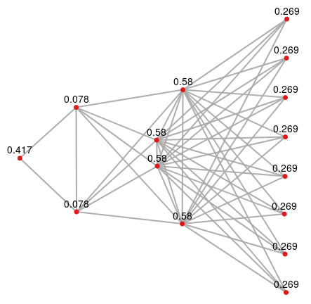
Figure 2: Normalized curvature ${\mathcal{K}}_{G,x}(\infty)$

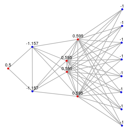
Figure 3: Non-normalized curvature ${\mathcal{K}}_{G,x}(\infty)$

Now we consider Ollivier-Ricci curvature. Here our main result is the following:

Theorem 1.6.

Let $G={\mathcal{AT}}((a_{k}))$ be an infinite antitree with $1=a_{1}$ and $a_{k+1}\geq a_{k}$ for all $k\in{\mathbb{N}}$ and $x,y$ be neighbouring vertices in $G$.

• Radial root edges: If $x\in V_{1}$ and $y\in V_{2}$:

  $$\kappa_{p}(x,y)=\begin{cases}\frac{a_{2}-1}{a_{2}+a_{3}}+\frac{a_{2}+2a_{3}+1}{a_{2}+a-3}p,&\text{if $p\in\left[0,\frac{1}{a_{2}+a_{3}+1}\right]$,}\\[5.69046pt] \frac{a_{2}+1}{a_{2}+a_{3}}(1-p),&\text{if $p\in\left[\frac{1}{a_{2}+a_{3}+1},1\right]$.}\end{cases}$$

• Radial edges: If $x\in V_{k}$ and $y\in V_{k+1}$, $k\geq 2$, $p\in[0,1]$:

  $$\kappa_{p}(x,y)=\left(\frac{2a_{k}+a_{k+1}-1}{a_{k}+a_{k+1}+a_{k+2}-1}-\frac{2a_{k-1}+a_{k}-1}{a_{k-1}+a_{k}+a_{k+1}-1}\right)(1-p).$$

• Spherical edges: If $x,y\in V_{k}$, $x\neq y$, $k\geq 2$:

  $$\kappa_{p}(x,y)=\begin{cases}\frac{a_{k-1}+a_{k}+a_{k+1}-2}{a_{k-1}+a_{k}+a_{k+1}-1}+\frac{a_{k-1}+a_{k}+a_{k+1}}{a_{k-1}+a_{k}+a_{k+1}-1}p,&\text{if $p\in\left[0,\frac{1}{a_{k-1}+a_{k}+a_{k+1}}\right]$,}\\[5.69046pt] \frac{a_{k-1}+a_{k}+a_{k+1}}{a_{k-1}+a_{k}+a_{k+1}-1}(1-p),&\text{if $p\in\left[\frac{1}{a_{k-1}+a_{k}+a_{k+1}},1\right]$.}\end{cases}$$

Let us consider special cases:

Corollary 1.7 (Linear growth).

Let $G={\mathcal{AT}}((1+(k-1)t))$, $t\in{\mathbb{N}}$ arbitrary. Then

$$\kappa_{0}(x,y)=\begin{cases}\frac{t}{3t+2}&\text{for $x\in V_{1}$, $y\in V_{2}$,}\\ \frac{6t^{2}}{(3kt+2)(3kt+2-3t)}&\text{for $x\in V_{k}$, $y\in V_{k+1}$,}\\ 1-\frac{1}{3kt+2-3t}&\text{for $x,y\in V_{k}$, $x\neq y$, $k\geq 2$.}\end{cases}$$

In particular, $\kappa_{0}$ of radial edges decays asymptotically like $\frac{2}{3k^{2}}$ as $k\to\infty$.

Corollary 1.8 (Exponential growth).

We have for $G={\mathcal{AT}}((r^{k-1})$, $r\in{\mathbb{N}}$:

$$\kappa_{0}(x,y)=\begin{cases}\frac{r-1}{r(r+1)}&\text{for $x\in V_{1}$, $y\in V_{2}$,}\\ \frac{(r-1)^{2}(r+1)r^{k-2}}{(r^{k}+r^{k-1}+r^{k-2}-1)(r^{k+1}+r^{k}+r^{k-1}-1)}&\text{for $x\in V_{k}$, $y\in V_{k+1}$,}\\ 1-\frac{1}{r^{k}+r^{k-1}+r^{k-2}-1}&\text{for $x,y\in V_{k}$, $x\neq y$, $k\geq 2$.}\end{cases}$$

In particular, $\kappa_{0}$ of radial edges decays asymptotically like $\frac{1}{r^{k}}$ as $k\to\infty$.

Remark 1.9.

Note that for any finite sequence $(a_{k})_{1\leq k\leq N}$, $N\geq 2$, with $1=a_{1}$ and $a_{k+1}\geq a_{k}$ for all $1\leq k\leq N$, we can find a large enough $a_{N+1}\geq a_{N}$ such that $\kappa_{0}(x,y)<0$ for $x\in V_{N-1}$ and $y\in V_{N}$.

The paper is organised as follows: We start with some historical comments on antitrees in Section 2 which was provided by Radosław Wojciechowski. Section 3 introduces the readers into Bakry-Émery curvature and Ollivier-Ricci curvature. The following two Sections 4 and 5 present the concrete curvature investigations in both settings. The Appendices A, B, and C provide the Maple code used for the results in Section 4.

Acknowledgement: We are grateful to Radoslaw Wojciechowski, Matthias Keller, and Jozef Dodziuk for providing useful information on antitrees. Some figures in this article are based on the curvature calculator by David Cushing and George Stagg (see [6]).

2 A (partial) history of antitrees

To our knowledge, the first known appearance of an antitree is the case of $|S_{r}|=r+1$ in the article of Dodziuk and Karp [8]. They study the normalized Laplacian $\Delta$ and give conditions for transience of the simple random walk in terms of $r\Delta r$ where $r$ is the distance to a vertex. It appears in [8, Example 2.5] as a case of a transient graph with bottom of the spectrum $0$ whose Green’s function decays like $1/r$. The same antitree appears in the article of Weber [24]. Weber extends the result of Dodziuk and Mathai [9] concerning the stochastic completeness of the semigroup associated to the non-normalized Laplacian $\Delta$. Indeed, Dodziuk/Mathai prove stochastic completeness in the case of bounded vertex degree. Weber improves this result to give stochastic completeness in the case of $\Delta r\geq K$ for some constant $K$. The antitree mentioned above is then given as an example of a graph whose vertex degree is unbounded but which satisfies $\Delta r\geq K$, see [24, Figure 1, p. 156]. The general case of antitrees with arbitrary spherical growth $|S_{r}|=f(r)$ where $f$ is any natural number valued function is considered in [25, Example 4.11]. There it is shown that antitrees are stochastically complete if and only if

$$\sum_{r}\frac{\sum_{k=0}^{r}f(k)}{f(r)f(r+1)}=\infty.$$

This is used to give a counterexample to a direct analogue to Grigor’yan’s result for stochastic completeness of manifolds (see [13]). Indeed, Grigor’yan’s result says that any stochastically incomplete manifold must have superexponential volume growth while the result above gives stochastically incomplete graphs which have only polynomial volume growth when the combinatorial graph metric is used. These examples give the smallest such examples in the combinatorial graph metric by a result of Huang, Grigor’yan and Masamune [12, Theorem 1.4], where the example (and name) of antitrees also appears. This might be the first time in print that the name is used and they refer to them as the ”antitree of Wojciechowski". A proper definition with the name of antitree first appears in [19, Definition 6.3]. Here the result on stochastic completeness is generalized to all weakly spherically symmetric graphs of which the antitrees are but an example. Furthermore, it is shown that the non-normalized Laplacian $\Delta$ on any such stochastically incomplete antitree has positive bottom of the spectrum, see [19, Corollary 6.6]. This gives a counterexample to a direct analogue to a theorem of Brooks [5] which states that the bottom of the spectrum of the Laplacian on any manifold with subexponential volume growth is zero. This sparked an interest in applying intrinsic metrics as defined by Frank, Lenz and Wingert in [10] to study the question involving volume growth on graphs of unbounded vertex degree. In particular, the analogue to Grigor’yan’s theorem was first proven in [11] (see also [18] for an analytic proof) while the analogue to Brooks’ theorem was shown in [16]. Since then, antitrees appear in a variety of places. Their spectral theory is thoroughly analyzed by Breuer and Keller in [4]. Here it should be noted that the spectrum consists mainly of eigenvalues with compactly supported eigenfunctions and a further spectral component which can be singular continuous in certain cases. Antitrees are also used as a counterexample to a conjecture presented by Golenia and Schumacher in [14] concerning the deficiency indices of the adjacency matrix, see [15]. They are also used to show the utility of the new bottom of the spectrum estimate for a Cheeger constant involving intrinsic metrics in [1].

3 Definitions and notations

3.1 Basic graph theoretical notations

Let $G=(V,E)$ be a locally finite connected simple combinatorial graph (that is, no loops and no multiple edges) with vertex set $V$ and edge set $E$. For any $x,y\in V$ we write $x\sim y$ if $\{x,y\}\in E$. The degree of a vertex $x\in V$ is denoted by $d_{x}$. Let $d:V\times V\to{\mathbb{N}}\cup\{0\}$ be the combinatorial distance function, i.e., $d(x,y)$ is the length of the shortest path from $x$ to $y$. For $x\in V$, the combinatorial spheres and balls of radius $r\geq 0$ around $x$ are denoted by

$$S_{r}(x) = \{y\in V\mid d(x,y)=r\},$$

$$B_{r}(x) = \{y\in V\mid d(x,y)\leq r\},$$

respectively. The diameter of $G$ is defined as

$${\rm{diam}}(G)=\sup\{d(x,y)\mid x,y\in V\}\in{\mathbb{N}}\cup\{0,\infty\}.$$

3.2 Bakry-Émery curvature

As mentioned before, this curvature notion is rooted on Bochner’s formula using a Laplacian operator leading to the curvature-dimension inequality (CD-inequality for short). This approach was pursued by Bakry-Émery [2] via an elegant $\Gamma$-calculus and lead to a substitute of the lower Ricci curvature bound of the underlying space for much more general settings. (Some further information on the Bochner approach can be found, e.g., in [7, Remark 1.3]).

Recall the definition (1.1) of the normalized ($\mu(x)=d_{x}$) and non-normalized Laplacian ($\mu\equiv 1$) from the Introduction. Such a choice of Laplacian leads to the following operator $\Gamma$ for all $f,g:V\to{\mathbb{R}}$:

$$\Gamma(f,g)(x) = \frac{1}{2}(\Delta(fg)-f\Delta g-g\Delta f)(x)$$

$$= \frac{1}{2\mu(x)}\sum_{y\sim x}(f(y)-f(x))(g(y)-g(x)).$$

For simplicity, we always write $\Gamma(f):=\Gamma(f,f)$. Iterating $\Gamma$, we can define another operator $\Gamma_{2}$, given by

$$\Gamma_{2}(f,g)(x)=\frac{1}{2}(\Delta\Gamma(f,g)-\Gamma(f,\Delta g)-\Gamma(g,\Delta f))(x).$$

Again, we abbreviate $\Gamma_{2}(f)=\Gamma_{2}(f,f)$. The Bakry-Émery curvature is defined via these operators in the following way.

Definition 3.1.

Let $K\in{\mathbb{R}}$ and $N\in(0,\infty]$.

1. The pointwise curvature dimension condition $CD(K,N,x)$ for $x\in V$ is defined by

   $$\Gamma_{2}(f)(x)\geq K\Gamma(f)(x)+\frac{1}{N}(\Delta f)^{2}(x),\,\,\,\text{for any }\,\,\,f:V\to\mathbb{R}.$$

2. The global curvature dimension condition $CD(K,N)$ holds if and only if $CD(K,N,x)$ holds for any $x\in V$.

3. For any $x\in V$, we define

   $${\mathcal{K}}_{G,x}(N):=\sup\{K\in{\mathbb{R}}\mid CD(K,N,x)\}.$$ (3.1)

In this article, we are only concerned with $\infty$-curvature, that is, $N=\infty$. Following [7, Prop. 2.1], the condition $CD(K,\infty,x)$ is equivalent to

$$\Gamma_{2}(x)\geq K\Gamma(x),$$ (3.2)

where $\Gamma_{2}(x)$ and $\Gamma(x)$ are symmetric matrices of the corresponding quadratic forms evaluated at $x\in V$. Since only local information needs to be taken into account, they are of size $|B_{2}(x)|\times|B_{2}(x)|$ and $|B_{1}(x)|\times|B_{1}(x)|$, respectively, and to make sense of (3.2) the smaller size matrix must be padded with $0$ entries. For more information in the non-normalized case, see [7, Sections 2.1-2.3]. The entries of these matrices in the general weighted case are explicitly given in [7, Section 12]. (Note that for the context of this article, the edge weights $w:E\to[0,\infty)$ take only values $0,1$ and reflect adjacency of vertices and the vertex measure $\mu:V\to(0,\infty)$ will only correspond to the normalized and non-normalized cases.)

The main tool to prove strictly positive curvature is [7, Corollary 2.7], that is, the following properties are equivalent:

• $\Gamma_{2}(x)$ is positive semidefinite with one-dimensional kernel,

• ${\mathcal{K}}_{G,x}(\infty)>0$.

[7, Corollary 2.7] covers only the non-normalized case but one can easily check that the equivalence holds also in the setting of general vertex measures.

3.3 Ollivier-Ricci curvature

As mentioned before, Ollivier-Ricci curvature is based on optimal transport. Ollivier-Ricci curvature was introduced in [23]. A fundamental concept in optimal transport is the Wasserstein distance between probability measures.

Definition 3.2.

Let $G=(V,E)$ be a locally finite graph. Let $\mu_{1},\mu_{2}$ be two probability measures on $V$. The Wasserstein distance $W_{1}(\mu_{1},\mu_{2})$ between $\mu_{1}$ and $\mu_{2}$ is defined as

$$W_{1}(\mu_{1},\mu_{2})=\inf_{\pi}\sum_{y\in V}\sum_{x\in V}d(x,y)\pi(x,y),$$ (3.3)

where the infimum runs over all transportation plans $\pi:V\times V\rightarrow[0,1]$ satisfying

$$\mu_{1}(x)=\sum_{y\in V}\pi(x,y),\>\>\>\mu_{2}(y)=\sum_{x\in V}\pi(x,y).$$

The transportation plan $\pi$ moves a mass distribution given by $\mu_{1}$ into a mass distribution given by $\mu_{2}$, and $W_{1}(\mu_{1},\mu_{2})$ is a measure for the minimal effort which is required for such a transition.

If $\pi$ attains the infimum in (3.3) we call it an optimal transport plan transporting $\mu_{1}$ to $\mu_{2}$.

We define the following probability distributions $\mu_{x}$ for any $x\in V,\>p\in[0,1]$:

$$\mu_{x}^{p}(z)=\begin{cases}p,&\text{if $z=x$,}\\ \frac{1-p}{d_{x}},&\text{if $z\sim x$,}\\ 0,&\mbox{otherwise.}\end{cases}$$

Definition 3.3.

The $p-$Ollivier-Ricci curvature on an edge $x\sim y$ in $G=(V,E)$ is

$$\kappa_{p}(x,y)=1-W_{1}(\mu^{p}_{x},\mu^{p}_{y}),$$

where $p\in[0,1]$ is called the idleness.

The Ollivier-Ricci curvature introduced by Lin-Lu-Yau in [20], is defined as

$$\kappa_{LLY}(x,y)=\lim_{p\rightarrow 1}\frac{\kappa_{p}(x,y)}{1-p}.$$

A fundamental concept in the optimal transport theory and vital to our work is Kantorovich duality. First we recall the notion of 1–Lipschitz functions and then state Kantorovich duality.

Definition 3.4.

Let $G=(V,E)$ be a locally finite graph, $\phi:V\rightarrow\mathbb{R}.$ We say that $\phi$ is $1$-Lipschitz if

$$|\phi(x)-\phi(y)|\leq d(x,y)$$

for all $x,y\in V.$ Let 1–Lip denote the set of all $1$–Lipschitz functions.

Note that, by triangle inequality, $\phi$ is $1$–Lipschitz iff $|\phi(x)-\phi(y)|\leq 1$ for all paris $x\sim y$.

Theorem 3.1 (Kantorovich duality).

Let $G=(V,E)$ be a locally finite graph. Let $\mu_{1},\mu_{2}$ be two probability measures on $V$. Then

$$W_{1}(\mu_{1},\mu_{2})=\sup_{\begin{subarray}{c}\phi:V\rightarrow\mathbb{R}\\ \phi\in\textrm{\rm{1}--{\rm Lip}}\end{subarray}}\sum_{x\in V}\phi(x)(\mu_{1}(x)-\mu_{2}(x)).$$

If $\phi\in\textrm{1--Lip}$ attains the supremum we call it an optimal Kantorovich potential transporting $\mu_{1}$ to $\mu_{2}$.

The following result on some properties of $p\mapsto\kappa_{p}(x,y)$ for $x\sim y$ and its consequences was useful in our curvature considerations.

Theorem 3.2 (see [3]).

Let $G=(V,E)$ be a locally finite graph. Let $x,y\in V$ with $x\sim y.$ Then the function $p\mapsto\kappa_{p}(x,y)$ is concave and piecewise linear over $[0,1]$ with at most $3$ linear parts. Furthermore $\kappa_{p}(x,y)$ is linear on the intervals

$$\left[0,\frac{1}{{\rm{lcm}}(d_{x},d_{y})+1}\right]\>\>\>{\rm and}\>\>\>\left[\frac{1}{\max(d_{x},d_{y})+1},1\right].$$

Thus, if we have the further condition $d_{x}=d_{y}$, then $\kappa_{p}(x,y)$ has at most two linear parts.

4 Bakry-Émery curvature of antitrees

Let us first introduce some notation and a useful general fact (Lemma 4.1 below). The identity matrix of size $d$ is denoted by ${\rm Id}_{d}$ and the all-zero and all-one matrix of size $d_{1}\times d_{2}$ is denoted by $0_{d_{1},d_{2}}$ and $J_{d_{1},d_{2}}$, respectively. Moreover, if $d_{1}=d_{2}$, we use the notation $J_{d_{1}}=J_{d_{1},d_{1}}$, and if $d_{2}=1$, we use the notation ${\bf 1}_{d_{1}}$ for the all-one column vector of size $d_{1}$. Moreover, the standard base of column vectors in ${\mathbb{R}}^{N}$ is denoted by $e_{1},\dots,e_{N}$.

Lemma 4.1.

Let $d_{1},\dots,d_{r}\in{\mathbb{N}}$ and $A=(A_{ij})_{1\leq i,j\leq r}$ be a symmetric matrix, where the $A_{ij}$ are block matrices of size $d_{i}\times d_{j}$ with $A_{ji}=A_{ij}^{\top}$. Assume there exist constants $\alpha_{i},\beta_{i}\in{\mathbb{R}}$ and $\gamma_{ij}=\gamma_{ji}\in{\mathbb{R}}$ such that, for $1\leq i,j\leq r$, $j\neq i$,

$$A_{ii}=\alpha_{i}{\rm Id}_{d_{i}}+\beta_{i}J_{d_{i}}$$

and

$$A_{ij}=\gamma_{ij}J_{d_{i},d_{j}}.$$

Let $A_{\rm{red}}=(a_{ij})_{1\leq i,j\leq r}$ be the $r\times r$-matrix given by $a_{ij}={\bf 1}_{d_{i}}^{\top}A_{ij}{\bf 1}_{d_{j}}$, i.e., for $i\neq j$,

$$a_{ii} = \alpha_{i}d_{i}+\beta_{i}d_{i}^{2},$$

$$a_{ij} = \gamma_{ij}d_{i}d_{j}.$$

For any vector $w=(w_{1},\dots,w_{r})^{\top}\in{\mathbb{R}}^{r}$ let

$$\widehat{w}:=(w_{1}{\bf 1}_{d_{1}}^{\top},\dots,w_{r}{\bf 1}_{d_{r}}^{\top})^{\top}\in{\mathbb{R}}^{d}$$

with $d=\sum_{j=1}^{r}d_{j}$. Then we have the following two facts:

• For every $d_{i}\geq 2$, the $(d_{i}-1)$-dimensional space

  $$E_{i}=\left\{\sum_{j=1}^{d_{i}}c_{j}e_{j+d}\mid\sum_{j=1}^{d_{i}}c_{j}=0\right\}$$

  with $d=\sum_{j=1}^{i-1}d_{j}$ consists of eigenvectors to the eigenvalue $\alpha_{i}$.

• For any $w\in{\mathbb{R}}^{r}$, the corresponding vector $\widehat{w}$ is orthogonal to all spaces $E_{i}$ in (a) and we have

  $${\widehat{w}}^{\top}A\widehat{\,}w=w^{\top}A_{\rm{red}}\,w.$$

The proof of this lemma is a straightforward calculation and left to the reader.

Now we start with our Bakry-Émery curvature considerations for antitrees. Due to localness of the Bakry-Émery curvature notion, we only need to consider ${\mathcal{K}}_{G,x}(\infty)$ for

• a vertex $x\in V_{3}$ in the finite antitree ${\mathcal{AT}}((a,b,c,d,e))$,

• a vertex $x\in V_{2}$ in the finite antitree ${\mathcal{AT}}((b,c,d,e))$, and

• a vertex $x\in V_{1}$ in the finite antitree ${\mathcal{AT}}((c,d,e))$.

The relevant results are given in the following theorems.

Theorem 4.2.

Let $x\in V_{3}$ be a vertex of the finite antitree $G={\mathcal{AT}}((a,b,c,d,e))$. If

$$a=n,\,\,b=n+1,\,\,c=n+2,\,\,d=n+3,\,\,\text{and}\,\,e=n+4,$$

we have in both the normalized and non-normalized case:

$${\mathcal{K}}_{G,x}(\infty)>0.$$ (4.1)

Proof.

In this proof, we will keep the values $a,b,c,d,e$ general as long as possible and only specify them towards the end of the proof. Let $G={\mathcal{AT}}((a,b,c,d,e))$, $1\leq a\leq b<c\leq d\leq e$ and $x\in V_{3}$. To cover simultaneously both the normalized and non-normalized setting, we choose

$$\epsilon_{-}=\frac{\mu(x)}{\mu(y_{-})}-1,\quad\epsilon_{+}=\frac{\mu(x)}{\mu(y_{+})}-1,$$

where $y_{-}\in V_{2}$ and $y_{+}\in V_{4}$. (Note that $\mu(z)$ depends only the generation of $z$.) Using the results in [7, Section 12], a tedious but straightforward calculation shows the following: The matrix $A=4\mu(x)^{2}\Gamma_{2}(x)$ is of the following block structure $A=(A_{ij})_{1\leq i,j\leq 6}$ where the blocks correspond to an ordering of $B_{2}(x)$ into the vertex sets $\{x\},V_{3}\backslash\{x\},V_{4},V_{2},V_{5},V_{1}$:

$$A_{11} = d_{x}(d_{x}+3)+3b\epsilon_{-}+3d\epsilon_{+},$$

$$A_{12} = (-(d_{x}+3)+b\epsilon_{-}+d\epsilon_{+})J_{1,c-1},$$

$$A_{13} = (-(d_{x}+3+e)-(2+c+e)\epsilon_{+})J_{1,d},$$

$$A_{14} = (-(d_{x}+3+a)-(2+a+c)\epsilon_{-})J_{1,b},$$

$$A_{15} = (d+d\epsilon_{+})J_{1,e},$$

$$A_{16} = (b+b\epsilon_{-})J_{1,a},$$

$$A_{22} = (3(d_{x}+1)+b\epsilon_{-}+d\epsilon_{+}){\rm{Id}}_{c-1}-2J_{c-1},$$

$$A_{23} = -(2+2\epsilon_{+})J_{c-1,d},$$

$$A_{24} = -(2+2\epsilon_{-})J_{c-1,b},$$

$$A_{25} = 0_{c-1,e},$$

$$A_{26} = 0_{c-1,a},$$

$$A_{33} = (-b+3c+3d+3e+(3c+4d+3e)\epsilon_{+}){\rm{Id}}_{d}-(2+4\epsilon_{+})J_{d},$$

$$A_{34} = 2J_{d,b},$$

$$A_{35} = -(2+2\epsilon_{+})J_{d,e},$$

$$A_{36} = 0_{d,a},$$

$$A_{44} = (3a+3b+3c-d+(3a+4b+3c)\epsilon_{-}){\rm{Id}}_{b}-(2+4\epsilon_{-})J_{b},$$

$$A_{45} = 0_{b,e},$$

$$A_{46} = -(2+2\epsilon_{-})J_{b,a},$$

$$A_{55} = (d+d\epsilon_{+}){\rm{Id}}_{e},$$

$$A_{56} = 0_{e,a},$$

$$A_{66} = (b+b\epsilon_{-}){\rm{Id}}_{a}.$$

Let $A_{\rm{red}}$ be the corresponding reduced symmetric $6\times 6$ matrix $A_{\rm{red}}=(a_{ij})_{1\leq i,j\leq 6}$, as defined in Lemma 4.1.

Recalling the equivalence at the end of Section 3.2, ${\mathcal{K}}_{G,x}(\infty)>0$ is equivalent to $A$ being positive semidefinite and having one-dimensional kernel. Lemma 4.1 provides the following eigenvalues and multiplicites of $A$:

• Since $\epsilon_{-},\epsilon_{+}>-1$ and $d_{x}=b+c+d-1$,

  $$\alpha_{2}=3(d_{x}+1_{+}b\epsilon_{-}+d\epsilon_{+})>0$$

  is a positive eigenvalue of multiplicity $c-2\geq 0$.

• Note that in both normalized and non-normalized case we have $\epsilon_{+}\geq\frac{b+c+d-1}{c+d+e-1}-1$ and

  $$\alpha_{3}=-b+3c+3d+3e+(3c+4d+3e)\epsilon_{+}\geq\\ \geq-b-d+\frac{3c+4d+3e}{c+d+e-1}(b+c+d-1)>0$$

  is a positive eigenvalue of multiplicity $d-1\geq 1$.

• Note that in both normalized and non-normalized case we have $\epsilon_{-}\geq 0$ and

  $$\alpha_{4}=3a+3b+3c-d+(3a+4b+3c)\epsilon_{-}\geq 3a+3b+3c-d>0$$

  if $d<3(a+b+c)$. This eigenvalue has multiplicity $b-1\geq 0$.

• Since $\epsilon_{-},\epsilon_{+}>-1$,

  $$\alpha_{5}=d+d\epsilon_{+}>0\quad\text{and}\,\,\alpha_{6}=b+b\epsilon_{-}>0$$

  are both positive eigenvalues of multiplicities $e-1\geq 1$ and $a-1\geq 0$, respectively.

Moreover, it is easily checked that $A{\bf 1}_{a+b+c+d+e}=0$. The orthogonal complement of the direct sum of the corresponding eigenspaces $E_{i}$ and ${\mathbb{R}}{\bf 1}_{a+b+c+d+e}$ is $5$-dimensional and given by $\widehat{W}=\{\widehat{w}\mid w\in W\}$, where $(d_{1},d_{2},d_{3},d_{4},d_{5},d_{6})=(1,c-1,d,b,e,a)$ and

$$W:=\{w\in{\mathbb{R}}^{6},\sum_{i=1}^{6}w_{i}d_{i}=0\}.$$

Under the assumption $d<3(a+b+c)$, ${\mathcal{K}}_{G,x}(\infty)>0$ is then equivalent to $A|_{\widehat{W}}$ being positive definite, which is equivalent to

$${\widehat{w}}^{\top}A\,\widehat{w}=w^{\top}A_{\rm{red}}\,w>0\quad\text{for all $w\in W\backslash\{0\}$.}$$ (4.2)

Now we choose $(a,b,c,d,e)=(n,n+1,n+2,n+3,n+4)$, $n\in{\mathbb{N}}$. Then we have $d<3(a+b+c)$ and we consider the characteristic polynomial of $A_{\rm{red}}$, which is of the form

$$\chi_{n}(t)=\det(t{\rm{Id}}_{6}-A_{\rm{red}})=t^{6}-p_{5}(n)t^{5}+p_{4}(n)t^{4}-p_{3}(n)t^{3}+p_{2}(n)t^{2}-p_{1}(n)t,$$

where $p_{i}(n)$ are polynomials in the variable $n$. (We do not have a constant term since ${\mathbb{R}}\cdot{\bf 1}_{6}$ lies in the kernel of $A_{\rm{red}}$.) A Maple calculation shows that all the $p_{i}(n)$ are strictly positive for any value of $n\in{\mathbb{N}}$ (see Appendix A for more details). This shows that we have $\chi_{n}(t)>0$ for all $t<0$, so $A_{\rm{red}}$ is positive semidefinite. Since $p_{1}(n)>0$, $A_{\rm{red}}$ has a one-dimensional kernel ${\mathbb{R}}\cdot{\bf 1}_{6}$.

Now we can show (4.2): Let $w_{0}={\bf 1}_{6},w_{1},\dots,w_{5}\in{\mathbb{R}}^{6}$ be a basis of eigenvectors of $A_{\rm{red}}$, i.e., $A_{\rm{red}}w_{j}=\lambda_{j}w_{j}$ with $\lambda_{j}>0$ for $j\in\{1,\dots,5\}$. Any vector $w\in W\backslash\{0\}$ is of the form $w=\sum_{j=0}^{5}c_{j}w_{j}$ with some $c_{j_{0}}\neq 0$, $j_{0}\in\{1,\dots,5\}$, since $w_{0}\not\in W$. This implies

$$w^{\top}A_{\rm{red}}\,w=\sum_{j=1}^{5}\lambda_{j}c_{j}^{2}\geq\lambda_{j_{0}}c_{j_{0}}^{2}>0.$$

∎

Theorem 4.3.

Let $x\in V_{2}$ be a vertex of the finite antitree $G={\mathcal{AT}}((b,c,d,e))$. If $(c,d,e)=(1,2,3)$, we have in both the normalized and non-normalized case:

$${\mathcal{K}}_{G,x}(\infty)>0.$$

Proof.

We consider again the matrix $A=4\mu(x)^{2}\Gamma_{2}(x)$ and choose right from the beginning $(b,c,d,e)=(1,2,3,4)$. It can be checked that this time the matrix $A$ is of the form $A=(A_{ij})_{1\leq i,j\leq 5}$ with $A_{ij}$ as in the previous proof and $a=0$. As in the previous proof, we conclude that $A$ has eigenvalues $\alpha_{3}=27+30\epsilon_{+}>0$ of multiplicity $2$ and $\alpha_{5}=1+\epsilon_{+}>0$ of multiplicity $3$ and that $A{\bf 1}_{10}=0$. In this case, $A_{\rm{red}}$ is a symmetric $5\times 5$ matrix and its characteristic polynomial of $A_{\rm{red}}$ is (see Maple calculations in Appendix B)

$$\chi(t)=\det(t{\rm{Id}}_{5}-A_{\rm{red}})=t^{5}-\frac{471}{4}t^{4}+\frac{118743}{32}t^{3}-\frac{593811}{16}t^{2}+\frac{3082725}{64}t$$

in the normalized case and

$$\chi(t)=t^{5}-132t^{4}+3684t^{3}-25632t^{2}+8640t$$

in the non-normalized case. The same arguments as in the previous proof show that $A$ is positive semidefinite with one-dimensional kernel, that is, ${\mathcal{K}}_{G,x}(\infty)>0$. ∎

Theorem 4.4.

Let $x\in V_{1}$ be a vertex of the finite antitree $G={\mathcal{AT}}(c,d,e)$. If $(c,d,e)=(1,2,3)$, we have in both the normalized and non-normalized case:

$${\mathcal{K}}_{G,x}(\infty)>0.$$

Proof.

As in the previous proof, we consider the matrix $A=4\mu(x)^{2}\Gamma_{2}(x)$ and choose $(c,d,e)=(1,2,3)$. This time $A$ is of the form $A=(A_{ij})_{i,j\in I}$ with $I=\{1,3,4\}$ and $A_{ij}$ as in the proof of Theorem 4.2 with $a=b=0$. As before, we conclude that $A$ has a simple eigenvalue $\alpha_{3}=18+20\epsilon_{+}>0$ and a double eigenvalue $\alpha_{5}=2+2\epsilon_{+}>0$ and $A{\bf 1}_{6}=0$. $A_{\rm{red}}$ is now a symmetric $3\times 3$ matrix with characteristic polynomial (see Maple calculations in Appendix B)

$$\chi(t)=t^{3}-\frac{112}{5}t^{2}+\frac{144}{5}t$$

in the normalized case and

$$\chi(t)=t^{3}-44t^{2}+72t$$

in the non-normalized case. Similarly as before, this implies that $A$ is positive semidefinite with one-dimensional kernel, that is, ${\mathcal{K}}_{G,x}(\infty)>0$. ∎

Remark 4.5.

Alternatively, Theorem 4.4 could be proved, in the non-normalized case, by employing the fact that the root of ${\mathcal{AT}}((1,2,3))$ is $S^{1}$-out regular. For the definition of this notion and the corresponding curvature calculation see [7, Definition 1.5 and Theorem 5.7].

The above theorems imply that the infinite antitree ${\mathcal{AT}}((k))$ has strictly positive Bakry-Émery curvature in all vertices. We finally prove that there is no uniform positive lower curvature bound.

Theorem 4.6.

Let $G={\mathcal{AT}}((k))$ be the infinite antitree with vertex set $V=\bigcup_{k=1}^{\infty}V_{k}$. Then we have both in the normalized and normalized setting

$$\inf_{x\in V}{\mathcal{K}}_{G,x}(\infty)=0.$$

Proof.

Let us first consider the normalized setting. If we had $\inf_{x\in V}{\mathcal{K}}_{G,x}(\infty)=K>0$, then the discrete Bonnet-Myers Theorem (Theorem 1.2 of the Introduction) would imply that $G$ has bounded diameter, which is a contradiction. This argument does not work in the non-normalized setting. Let us now show in the non-normalized setting that

$$\lim_{n\to\infty,x\in V_{n}}{\mathcal{K}}_{G,x}(\infty)=0.$$

For $\delta>0$, let $A(\delta,n)=4(\Gamma_{2}(x)-\delta\Gamma(x))$ for an arbitrary vertex $x\in V_{n+2}$, $n\in{\mathbb{N}}$, with respect to the vertex order

$$B_{2}(x)=\{x\}\ \sqcup(V_{n+2}\backslash\{x\})\sqcup V_{n+3}\sqcup V_{n+1}\sqcup V_{n+4}\sqcup V_{n}.$$

The entries of $2\Gamma(x)$ in the non-normalized setting are given in [7, (2.2)], and using this information, we see that that matrix $A(\delta,n)$ is of the following block structure $A(\delta,n)=(A_{ij}(\delta,n))_{1\leq i,j\leq 6}$:

$$A_{11}(\delta,n) = (3n+5)(3n+8)-(6n+10)\delta,$$

$$A_{12}(\delta,n) = (-3n-8+2\delta)J_{1,n+1},$$

$$A_{13}(\delta,n) = (-4n-12+2\delta)J_{1,n+3},$$

$$A_{14}(\delta,n) = (-4n-8+2\delta)J_{1,n+1},$$

$$A_{15}(\delta,n) = (n+3)J_{1,n+4},$$

$$A_{16}(\delta,n) = (n+1)J_{1,n},$$

$$A_{22}(\delta,n) = (9n+18-2\delta){\rm{Id}}_{n+1}-2J_{n+1},$$

$$A_{23}(\delta,n) = -2J_{n+1,n+3},$$

$$A_{24}(\delta,n) = -2J_{n+1,n+1},$$

$$A_{25}(\delta,n) = 0_{n+1,n+4},$$

$$A_{26}(\delta,n) = 0_{n+1,n},$$

$$A_{33}(\delta,n) = (8n+26-2\delta){\rm{Id}}_{n+3}-2J_{n+3},$$

$$A_{34}(\delta,n) = 2J_{n+3,n+1},$$

$$A_{35}(\delta,n) = -2J_{n+3,n+4},$$

$$A_{36}(\delta,n) = 0_{n+3,n},$$

$$A_{44}(\delta,n) = (8n+6-2\delta){\rm{Id}}_{n+1}-2J_{n+1},$$

$$A_{45}(\delta,n) = 0_{n+1,n+4},$$

$$A_{46}(\delta,n) = -2J_{n+1,n},$$

$$A_{55}(\delta,n) = (n+3){\rm{Id}}_{n+4},$$

$$A_{56}(\delta,n) = 0_{n+4,n},$$

$$A_{66}(\delta,n) = (n+1){\rm{Id}}_{n}.$$

Let $\delta>0$. Let $\lambda_{j}(\delta,n)$, $j\in\{1,\dots,5\}$ be the eigenvalues of the $6\times 6$ matrix $A(\delta,n)_{red}$. The characteristic polynomial of $A(\delta,n)_{red}$ is of the form

$$\chi_{\delta,n}(t)=t^{6}-p_{5}(\delta,n)t^{5}+p_{4}(\delta,n)t^{4}-p_{3}(\delta,n)t^{3}+p_{2}(\delta,n)t^{2}-p_{1}(\delta,n)t,$$

with polynomials $p_{1},p_{2},\dots,p_{5}$, and a Maple calculation shows that

$$p_{1}(\delta,n)=-240\delta n^{9}+q_{8}(\delta)n^{8}+\dots+q_{1}(\delta)n+q_{0}(\delta),$$ (4.3)

with polynomials $q_{0},q_{1},\dots,q_{8}$ (see Appendix C). By Vieta’s formulas, we have

$$p_{1}(\delta,n)=\left(\prod_{j=1}^{5}\lambda_{j}(\delta,n)\right),$$

where $\lambda_{j}(\delta,n)$, $j=1,\dots,5$ are the eigenvalues (in ascending order) of $A(\delta,n)_{red}$ restricted to the orthogonal complement to the eigenvector ${\bf 1}_{6}$. We conclude from (4.3) that there exists $k_{0}>0$ with $p_{1}(\delta,n)<0$ for all $n\geq n_{0}$, i.e., $\lambda_{1}(\delta,n)<0$. Applying Lemma 4.1, we conclude

$$(\widetilde{w})^{\top}A(\delta,n)\widetilde{w}=w^{\top}A(\delta,n)_{red}w=\lambda_{1}(\delta,n)\|w\|^{2}<0.$$

This implies that ${\mathcal{K}}_{G,x}(\infty)\in(0,\delta)$ for every $x\in V_{n+2}$ with $n\geq n_{0}$. ∎

5 Ollivier Ricci curvature of antitrees

In this section, we calculate Ollivier-Ricci curvature for all idlenesses $p\in[0,1]$ and the Lin-Lu-Yau curvature of all types of edges in antitrees.

Theorem 5.1 (Radial root-edges of an antitree).

Let $1\leq a\leq b\leq c,$ $\{x,y\}$ a radial root edge of the antitree $\mathcal{AT}((a,b,c)),$ that is $x\in V_{1},y\in V_{2}.$ Then we have:

1. If $a=1,$
   $\kappa_{p}(x,y)=\begin{cases}\frac{b-1}{b+c}+\frac{b+2c+1}{b+c}p&\text{if $p\in[0,\frac{1}{b+c+1}]$,}\\ \frac{b+1}{b+c}(1-p),&\text{if $p\in[\frac{1}{b+c+1},1]$.}\end{cases}$
   Therefore,

   $$\kappa_{LLY}(x,y)=\frac{b+1}{b+c}.$$

2. If $a\geq 3$ or $(a=2\>{\rm and}\>b<c),$
   $\kappa_{p}(x,y)=$
   $\frac{1}{(a+b-1)(a+b+c-1)}\begin{cases}((a+b-1)^{2}-c(a-1))+c(b+2a-2)p&\text{if $p\in[0,\frac{1}{a+b+c}]$,}\\ ((a+b)(a+b-1)-c(a-1))(1-p),&\text{if $p\in[\frac{1}{a+b+c},1]$.}\end{cases}$
   Therefore,

   $$\kappa_{LLY}(x,y)=\frac{(a+b)(a+b-1)-c(a-1)}{(a+b-1)(a+b+c-1)}.$$

3. If $a=2,b=c,$
   $\kappa_{p}(x,y)=\begin{cases}\frac{b}{2b+1}+\frac{3b+2}{2b+1}p&\text{if $p\in[0,\frac{1}{(2b+1)(b+1)1}]$,}\\ \frac{b^{2}+b+1}{(2b+1)(b+1)}+\frac{b^{2}+2b}{(2b+1)(b+1)}p,&\text{if $p\in[\frac{1}{(2b+1)(b+1)+1},\frac{1}{2(b+1)}]$,}\\ \frac{b^{2}+2b+2}{(2b+1)(b+1)}(1-p),&\text{if $p\in[\frac{1}{2(b+1)},1]$.}\end{cases}$
   Therefore,

   $$\kappa_{LLY}(x,y)=\frac{b^{2}+2b+2}{(2b+1)(b+1)}.$$

Proof.

1. Consider the following graph

   with associated probability measures $\mu^{p}_{1},\mu^{p}_{2},$ defined as

   $$\mu^{p}_{1}(x^{\prime})=p,\>\>\mu^{p}_{1}(y^{\prime})=\frac{1}{b}(1-p),\>\>\mu^{p}_{1}(v)=\frac{b-1}{b}(1-p),\>\>\mu^{p}_{1}(z)=0,$$

   $$\mu^{p}_{2}(x^{\prime})=\frac{1}{b+c}(1-p),\>\>\mu^{p}_{2}(y^{\prime})=p,\>\>\mu^{p}_{2}(v)=\frac{b-1}{b+c}(1-p),\>\>\mu^{p}_{2}(z)=\frac{c}{b+c}(1-p).$$

   One can verify that, due to the high connectivity of $\mathcal{AT}((a,b,c)),$ we have $W_{1}(\mu^{p}_{x},\mu^{p}_{y})=W_{1}(\mu^{p}_{1},\mu^{p}_{2}),$ where $x^{\prime}$ represents the root $x$, $y^{\prime}$ represents the vertex $y$, the vertex $v$ represents all neighbours of $y$ in $V_{2},$ and the vertex $z$ represents all vertices in $V_{3}.$
   
   Note that $\mu_{1}^{p}(x^{\prime})<\mu_{2}^{p}(x^{\prime})$ if and only if $p<\frac{1}{b+c+1}.$ We will distinguish the cases.
   
   Case $p<\frac{1}{b+c+1}:$
   Note that

   $$\mu_{1}^{p}(x^{\prime})<\mu_{2}^{p}(x^{\prime}),\>\>\>\mu_{1}^{p}(z)<\mu_{2}^{p}(z),$$

   $$\mu_{1}^{p}(y^{\prime})>\mu_{2}^{p}(y^{\prime}),\>\>\>\mu_{1}^{p}(w)>\mu_{2}^{p}(w).$$

   Thus when transporting $\mu_{1}^{p}$ to $\mu_{2}^{p}$ the only vertices that gain mass are $x^{\prime}$ and $z.$ Note further all this mass can be transported over a distance of $1$. Thus

   $$W_{1}(\mu^{p}_{x},\mu^{p}_{y}) =W_{1}(\mu^{p}_{1},\mu^{p}_{2})$$

   $$\leq\mu_{2}^{p}(x^{\prime})+\mu_{2}^{p}(z)-\mu_{1}^{p}(x^{\prime})-\mu_{1}^{p}(z)$$

   $$=\frac{c+1}{b+c}-\frac{b+2c+1}{b+c}p.$$

   We verify that this is in fact equality by constructing the following $\phi\in 1-$Lip,

   $$\phi(x^{\prime})=0,\phi(y^{\prime})=1,\phi(w)=1,\phi(z)=0.$$

   Then, by Theorem 3.1,

   $$W_{1}(\mu^{p}_{x},\mu^{p}_{y})=W_{1}(\mu^{p}_{1},\mu^{p}_{2})\geq\sum_{v}\phi(v)(\mu^{p}_{1}(v)-\mu^{p}_{2}(v))=\frac{c+1}{b+c}-\frac{b+2c+1}{b+c}p.$$

   Therefore

   $$W_{1}(\mu^{p}_{x},\mu^{p}_{y})=\frac{c+1}{b+c}-\frac{b+2c+1}{b+c}p.$$

   and

   $$\kappa_{p}(x,y)=\frac{b-1}{b+c}+\frac{b+2c+1}{b+c}p,$$ (5.1)

   for $p\in[0,\frac{1}{b+c+1}).$ By continuity of $p\mapsto\kappa_{p}(x,y)$ this also holds for $p=\frac{1}{b+c+1}.$
   
   Case $p\geq\frac{1}{b+c+1}:$
   By [3, Theorem 4.4], $\kappa_{p}(x,y)=\frac{b+c+1}{b+c}\kappa_{\frac{1}{b+c+1}}(1-p)$ for $p\in[\frac{1}{b+c+1},1].$ Thus

   $$\kappa_{p}(x,y)=\begin{cases}\frac{b-1}{b+c}+\frac{b+2c+1}{b+c}p&\text{if $p\in[0,\frac{1}{b+c+1}]$,}\\ \frac{b+c+1}{b+c}\kappa_{\frac{1}{b+c+1}}(1-p),&\text{if $p\in[\frac{1}{b+c+1},1]$.}\end{cases}$$

   Therefore it only remains to show that $\frac{b+c+1}{b+c}\kappa_{\frac{1}{b+c+1}}=\frac{b+1}{b+c}.$
   
   We have, using (5.1),

   $$\frac{b+c+1}{b+c}\kappa_{\frac{1}{b+c+1}} =\frac{b+c+1}{b+c}\left(\frac{b-1}{b+c}+\frac{b+2c+1}{b+c}\frac{1}{b+c+1}\right)$$

   $$=\frac{b+1}{b+c}.$$

2. Similar to above we consider the simplified graph representing $\mathcal{AT}((a,b,c)),$

   with associated probability measures $\mu^{p}_{1},\mu^{p}_{2},$ defined as

   $$\mu^{p}_{1}(x^{\prime})=p,\>\>\mu^{p}_{1}(y^{\prime})=\frac{1}{a+b-1}(1-p),\>\>\mu^{p}_{1}(u)=\frac{a-1}{a+b-1}(1-p),$$

   $$\mu^{p}_{1}(v)=\frac{b-1}{a+b-1}(1-p),\>\>\mu^{p}_{1}(z)=0,$$

   $$\mu^{p}_{2}(x^{\prime})=\frac{1}{a+b+c-1}(1-p),\>\>\mu^{p}_{2}(y^{\prime})=p,\>\>\mu^{p}_{2}(u)=\frac{a-1}{a+b+c-1}(1-p),$$

   $$\mu^{p}_{2}(v)=\frac{b-1}{a+b+c-1}(1-p),\>\>\mu^{p}_{2}(z)=\frac{c}{a+b+c-1}(1-p).$$

   Again, one can verify that, due to the high connectivity of $\mathcal{AT}((a,b,c)),$ we have $W_{1}(\mu^{p}_{x},\mu^{p}_{y})=W_{1}(\mu^{p}_{1},\mu^{p}_{2}),$ where $x^{\prime}$ represents the root $x$, $y^{\prime}$ represents the vertex $y$, the vertex $u$ represents all neighbours of $x$ in $V_{1},$ the vertex $v$ represents all neighbours of $y$ in $V_{2},$ and the vertex $z$ represents all vertices in $V_{3}.$
   
   Let $p\in(0,\frac{1}{a+b+c}).$ One can check that

   $$\mu_{1}^{p}(x^{\prime})<\mu_{2}^{p}(x^{\prime}),\>\>\mu_{1}^{p}(z)<\mu_{2}^{p}(z),$$

   $$\mu_{1}^{p}(y^{\prime})>\mu_{2}^{p}(y^{\prime}),\>\>\mu_{1}^{p}(u)>\mu_{2}^{p}(u),\>\>\mu_{1}^{p}(v)>\mu_{2}^{p}(v).$$

   Thus the vertices $x^{\prime}$ and $z$ must gain mass and the vertices $u,v$ and $y$ must lose mass. We now show that some mass must be transported from $u$ to $z$. Suppose that no mass is moved from $u$ to $v$. Then the mass available to move from $v$ and $y^{\prime}$ will be sufficient when moved to $z$. Therefore

   $$\mu_{1}^{p}(y^{\prime})+\mu_{1}^{p}(v)-\mu_{2}^{p}(y^{\prime})-\mu_{2}^{p}(v)\geq\mu_{2}^{p}(z)-\mu_{1}^{p}(z).$$

   Substituting in the values of the measures and rearranging gives $p\leq\frac{a+b+c-ac-1}{(a+b)(a+b-1)+bc}\leq 0,$ a contradiction. Therefore some mass must be transported from $u$ to $z$ over a distance of $2$ and all other mass can be transported over a distance of $1$.
   
   Thus

   $$W_{1}(\mu^{p}_{x},\mu^{p}_{y})= W_{1}(\mu^{p}_{1},\mu^{p}_{2})$$

   $$\leq (\mu_{2}^{p}(x)-\mu_{1}^{p}(x))+2(\mu^{p}_{1}(u)-\mu^{p}_{2}(u)-(\mu_{2}^{p}(x)-\mu_{1}^{p}(x)))$$

   $$+(\mu^{p}_{1}(y^{\prime})+\mu^{p}_{1}(v)-\mu^{p}_{2}(y^{\prime})-\mu^{p}_{2}(v))$$

   $$= (1-p)\left(\frac{a-1}{a+b-1}+\frac{c+1-a}{a+b+c-1}\right).$$

   We verify that this is in fact equality by constructing the following $\phi\in 1-$Lip,

   $$\phi(x^{\prime})=0,\phi(y^{\prime})=0,\phi(u)=1,\phi(v)=0,\phi(z)=-1.$$

   Therefore

   $$\kappa_{p}(x,y) =1-(1-p)\left(\frac{a-1}{a+b-1}+\frac{c+1-a}{a+b+c-1}\right)$$

   $$=\frac{((a+b-1)^{2}-c(a-1))+(bc+2c(a-1))p}{(a+b-1)(a+b+c-1)},$$

   for $p\in(0,\frac{1}{a+b+c}).$
   
   As before, by [3, Theorem 4.4], $\kappa_{p}(x,y)=\frac{a+b+c}{a+b+c-1}\kappa_{\frac{1}{a+b+c}}(1-p)$ for $p\in[\frac{1}{a+b+c},1].$ Therefore

   $$\frac{a+b+c}{a+b+c-1}\kappa_{\frac{1}{a+b+c}}=\frac{(a+b)(a+b-1)-c(a-1)}{(a+b-1)(a+b+c-1)},$$

   thus completing the proof.

3. As in part (b) we consider the simplified graph representing $\mathcal{AT}((a,b,c)),$

   with the same associated probability measures $\mu^{p}_{1},\mu^{p}_{2},$ defined as

   $$\mu^{p}_{1}(x^{\prime})=p,\>\>\mu^{p}_{1}(y^{\prime})=\frac{1}{a+b-1}(1-p),\>\>\mu^{p}_{1}(u)=\frac{a-1}{a+b-1}(1-p),$$

   $$\mu^{p}_{1}(v)=\frac{b-1}{a+b-1}(1-p),\>\>\mu^{p}_{1}(z)=0,$$

   $$\mu^{p}_{2}(x^{\prime})=\frac{1}{a+b+c-1}(1-p),\>\>\mu^{p}_{2}(y^{\prime})=p,\>\>\mu^{p}_{2}(u)=\frac{a-1}{a+b+c-1}(1-p),$$

   $$\mu^{p}_{2}(v)=\frac{b-1}{a+b+c-1}(1-p),\>\>\mu^{p}_{2}(z)=\frac{c}{a+b+c-1}(1-p).$$

   Again, one can verify that, due to the high connectivity of $\mathcal{AT}((a,b,c)),$ we have $W_{1}(\mu^{p}_{x},\mu^{p}_{y})=W_{1}(\mu^{p}_{1},\mu^{p}_{2}),$ where $x^{\prime}$ represents the root $x$, $y^{\prime}$ represents the vertex $y$, the vertex $u$ represents all neighbours of $x$ in $V_{1},$ the vertex $v$ represents all neighbours of $y$ in $V_{2},$ and the vertex $z$ represents all vertices in $V_{3}.$
   
   We will distinguish the cases.
   
   Case $p\in(0,\frac{1}{(2b+1)(b+1)1}):$
   One can check that

   $$\mu_{1}^{p}(x^{\prime})<\mu_{2}^{p}(x^{\prime}),\>\>\mu_{1}^{p}(z)<\mu_{2}^{p}(z),$$

   $$\mu_{1}^{p}(y^{\prime})>\mu_{2}^{p}(y^{\prime}),\>\>\mu_{1}^{p}(u)>\mu_{2}^{p}(u),\>\>\mu_{1}^{p}(v)>\mu_{2}^{p}(v),$$

   and

   $$\mu_{1}^{p}(y^{\prime})+\mu_{1}^{p}(v)-\mu_{2}^{p}(y^{\prime})-\mu_{2}^{p}(v)\geq\mu_{2}^{p}(z)-\mu_{1}^{p}(z).$$

   Thus the vertices $x^{\prime}$ and $z$ must gain mass and the vertices $u,v$ and $y.$ must lose mass and it is possible for all mass to be moved over a distance of $1$.
   
   Thus

   $$W_{1}(\mu^{p}_{x},\mu^{p}_{y}) =W_{1}(\mu^{p}_{1},\mu^{p}_{2})$$

   $$\leq\mu_{2}^{p}(x^{\prime})+\mu_{2}^{p}(z)-\mu_{1}^{p}(x^{\prime})-\mu_{1}^{p}(z)$$

   $$=\frac{b+1}{2b+1}-\frac{3b+2}{2b+1}p.$$

   We verify that this is in fact equality by constructing the following $\phi\in 1-$Lip,

   $$\phi(x^{\prime})=-1,\phi(y^{\prime})=0,\phi(u)=0,\phi(v)=0,\phi(z)=-1.$$

   Therefore

   $$\kappa_{p}(x,y)=\frac{b}{2b+1}+\frac{3b+2}{2b+1}p.$$

   Case $p\in(\frac{1}{(2b+1)(b+1)+1},\frac{1}{2(b+1)}):$
   One can check that we still have

   $$\mu_{1}^{p}(x^{\prime})<\mu_{2}^{p}(x^{\prime}),\>\>\mu_{1}^{p}(z)<\mu_{2}^{p}(z),$$

   $$\mu_{1}^{p}(y^{\prime})>\mu_{2}^{p}(y^{\prime}),\>\>\mu_{1}^{p}(u)>\mu_{2}^{p}(u),\>\>\mu_{1}^{p}(v)>\mu_{2}^{p}(v)$$

   However we now have

   $$\mu_{1}^{p}(y^{\prime})+\mu_{1}^{p}(v)-\mu_{2}^{p}(y^{\prime})-\mu_{2}^{p}(v)\leq\mu_{2}^{p}(z)-\mu_{1}^{p}(z).$$

   Thus, as in part (b), some mass must be transported from $u$ to $z$ over a distance of $2$ and all other mass can be transported over a distance of $1$.
   
   Therefore

   $$W_{1}(\mu^{p}_{x},\mu^{p}_{y})= W_{1}(\mu^{p}_{1},\mu^{p}_{2})$$

   $$\leq (\mu_{2}^{p}(x)-\mu_{1}^{p}(x))+2(\mu^{p}_{1}(u)-\mu^{p}_{2}(u)-(\mu_{2}^{p}(x)-\mu_{1}^{p}(x)))$$

   $$+(\mu^{p}_{1}(y^{\prime})+\mu^{p}_{1}(v)-\mu^{p}_{2}(y^{\prime})-\mu^{p}_{2}(v))$$

   $$= (1-p)\left(\frac{1}{b+1}+\frac{b-1}{2b+1}\right).$$

   We verify that this is in fact equality by constructing the following $\phi\in 1-$Lip,

   $$\phi(x^{\prime})=0,\phi(y^{\prime})=0,\phi(u)=1,\phi(v)=0,\phi(z)=-1.$$

   Therefore

   $$\kappa_{p}(x,y)=\frac{b^{2}+b+1}{(2b+1)(b+1)}+\frac{b^{2}+2b}{(2b+1)(b+1)}p.$$

   Case $p\in(\frac{1}{2(b+1)},1):$ As before, by [3, Theorem 4.4], $\kappa_{p}(x,y)=\frac{2(b+1)}{2b+1}\kappa_{\frac{1}{2(b+1)}}(1-p)$ for $p\in[\frac{1}{2(b+1)},1].$ Thus

   $$\frac{2(b+1)}{2b+1}\kappa_{\frac{1}{2(b+1)}}=\frac{b^{2}+2b+2}{(2b+1)(b+1)},$$

   thus completing the proof.

∎

Theorem 5.2 (Inner radial edges of an antitree).

Let $1\leq a\leq b\leq c\leq d,$ $\{x,y\}$ an inner radial edge of the antitree $\mathcal{AT}((a,b,c,d)),$ that is $x\in V_{2},y\in V_{3}.$ Then we have:

$$\kappa_{p}(x,y)=\left(\frac{2b+c-1}{b+c+d-1}-\frac{2a+b-1}{a+b+c-1}\right)(1-p).$$

Proof.

We first calculate $\kappa_{0}(x,y).$ We consider the simplified graph representing $\mathcal{AT}((a,b,c,d)),$

with the associated probability measures $\mu_{1},\mu_{2},$ defined as

$$\mu_{1}(x^{\prime})=0,\>\>\mu_{1}(y^{\prime})=\frac{1}{a+b+c-1},\>\>\mu_{1}(w)=\frac{a}{a+b+c-1},$$

$$\mu_{1}(u)=\frac{b-1}{a+b+c-1},\>\>\mu_{1}(v)=\frac{c-1}{a+b+c-1},\>\>\mu_{1}(z)=0,$$

$$\mu_{2}(x^{\prime})=\frac{1}{b+c+d-1},\>\>\mu_{2}(y^{\prime})=0,\>\>\mu_{2}(w)=0,$$

$$\mu_{2}(u)=\frac{b-1}{b+c+d-1},\>\>\mu_{2}(v)=\frac{c-1}{b+c+d-1},\>\>\mu_{2}(z)=\frac{d}{b+c+d-1}.$$

Again, one can verify that, due to the high connectivity of $\mathcal{AT}((a,b,c,d)),$ we have $W_{1}(\mu^{0}_{x},\mu^{0}_{y})=W_{1}(\mu_{1},\mu_{2}),$ where $x^{\prime}$ represents the vertex $x$, $y^{\prime}$ represents the vertex $y$, the vertex $w$ represents all the vertices in $V_{1},$ the vertex $u$ represents all neighbours of $x$ in $V_{2},$ the vertex $v$ represents all neighbours of $y$ in $V_{3},$ and the vertex $z$ represents all vertices in $V_{4}.$

Observe that

$$\mu_{1}(x^{\prime})<\mu_{2}(x^{\prime}),\>\>\mu_{1}(z)<\mu_{2}(z),\>\>\mu_{1}(u)<\mu_{2}(u),\>\>\mu_{1}(v)<\mu_{2}(v),$$

$$\mu_{1}(y^{\prime})>\mu_{2}(y^{\prime}),\>\>\mu_{1}(w)>\mu_{2}(w).$$

Therefore the only vertices that gain mass are $x^{\prime}$ and $z.$ Now, $\mu_{1}(w)-\mu_{2}(w)=\frac{a}{a+b+c-1}\geq\frac{1}{b+c+d-1}=\mu_{2}(x^{\prime})-\mu_{1}(x^{\prime}),$ and so it is possible for $x^{\prime}$ to receive all of its needed mass from $w.$ If we do this plan and send all other surplus mass to the vertex $z$ we obtain

$$W_{1}(\mu^{p}_{x},\mu^{p}_{y})= W_{1}(\mu^{p}_{1},\mu^{p}_{2})$$

$$\leq (\mu_{2}(x^{\prime})-\mu_{1}(x^{\prime}))+3(\mu_{1}(w)-[\mu_{2}(x^{\prime})-\mu_{1}(x^{\prime})]-\mu_{2}(w))+2(\mu_{1}(u)-\mu_{2}(u))$$

$$+(\mu_{1}(v)-\mu_{2}(v))+(\mu_{1}(y^{\prime})-\mu_{2}(y^{\prime}))$$

$$= \frac{3a+2b+c-2}{a+b+c-1}-\frac{2b+c-1}{b+c+d-1}.$$

We verify that this is in fact equality by constructing the following $\phi\in 1-$Lip,

$$\phi(w)=3,\>\>\phi(x^{\prime})=2,\>\>\phi(u)=2,\>\>\phi(y^{\prime})=1,\>\>\phi(v)=1,\>\>\phi(z)=0.$$

Thus

$$\kappa_{0}(x,y)=\frac{2b+c-1}{b+c+d-1}-\frac{2a+b-1}{a+b+c-1}.$$

Observe that $\phi(x^{\prime})-\phi(y^{\prime})=1$ and thus, by [3, Lemma 4.2], we have that $p\mapsto\kappa_{p}(x,y)$ is linear. Since $\kappa_{1}(x,y)=0,$ this gives

$$\kappa_{p}(x,y)\left(\frac{2b+c-1}{b+c+d-1}-\frac{2a+b-1}{a+b+c-1}\right)(1-p).$$

∎

Theorem 5.3 (Spherical root edges of an antitree).

Let $2\leq a\leq b,$ $\{x,y\}$ a spherical root edge of the antitree $\mathcal{AT}((a,b)),$ that is $x,y\in V_{1}.$ Then

$$\kappa_{p}(x,y)=\begin{cases}\frac{a+b-2}{a+b-1}+\frac{a+b}{a+b-1}p&\text{if $p\in[0,\frac{1}{a+b}]$,}\\ \frac{a+b}{a+b-1}(1-p),&\text{if $p\in[\frac{1}{a+b},1]$.}\end{cases}$$

Proof.

Since $d_{x}=d_{y},$ by [3, Theorem 5.3], we have

$$\kappa_{p}(x,y)=\begin{cases}((a+b-1)\kappa_{LLY}(x,y)-(a+b)\kappa_{0}(x,y))p+\kappa_{0}(x,y),&\text{if $p\in[0,\frac{1}{a+b}]$,}\\ (1-p)\kappa_{LLY}(x,y),&\text{if $p\in[\frac{1}{a+b},1]$.}\end{cases}$$

Therefore we will calculate $\kappa_{p}(x,y)$ for $p=0$ and $p=\frac{1}{a+b}.$

Observe that $\mu_{x}^{0}(y)=\frac{1}{a+b-1}$ and $0$ otherwise, and $\mu_{y}^{0}(x)=\frac{1}{a+b-1}$ and $0$ otherwise. Thus we have

$$W_{1}(\mu_{x}^{0},\mu_{y}^{0})=\frac{1}{a+b-1},$$

and so

$$\kappa_{0}(x,y)=\frac{a+b-2}{a+b-1}.$$

Note that

$$\mu_{x}^{\frac{1}{a+b}}\equiv\mu_{y}^{\frac{1}{a+b}},$$

so

$$\kappa_{LLY}(x,y)=\frac{a+b}{a+b-1}\kappa_{\frac{1}{a+b}}(x,y)=\frac{a+b}{a+b-1}.$$

Substituting these values in to the above formula completes the proof. ∎

Theorem 5.4 (Spherical inner edges of an antitree).

Let $1\leq a\leq b\leq c,$ $\{x,y\}$ a spherical inner edge of the antitree $\mathcal{AT}((a,b,c)),$ that is $x,y\in V_{2}.$ Then

$$\kappa_{p}(x,y)=\begin{cases}\frac{a+b+c-2}{a+b+c-1}+\frac{a+b+c}{a+b+c-1}p&\text{if $p\in[0,\frac{1}{a+b+c}]$,}\\ \frac{a+b+c}{a+b+c-1}(1-p),&\text{if $p\in[\frac{1}{a+b+c},1]$.}\end{cases}$$

Proof.

The proofs follows in the same way as in the proof of Theorem 5.3. ∎

Appendix A Maple Calculations for Theorem 4.2

In the normalized case, the Maple code to construct the matrix $A_{\rm{red}}=4\mu_{x}^{2}\Gamma_{2,\rm{red}}(x)$ for $x\in V_{3}\cong K_{c}$ of ${\mathcal{AT}}((a,b,c,d,e))$ is the following:

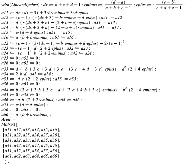
Figure 4: Maple construction of $A_{\rm{red}}$ in the normalized case

For the generation of the coefficients of the charactestic polynomial $\chi_{n}(t)$ of $A_{\rm{red}}$ for $a=n,b=n+1,c=n+2,d=n+3,e=n+4$, see Figure 5. Note that there are no negative coefficients in the polynomials $p_{1}(n),p_{2}(n),p_{3}(n),p_{4}(n)$ and $p_{5}(n)$.

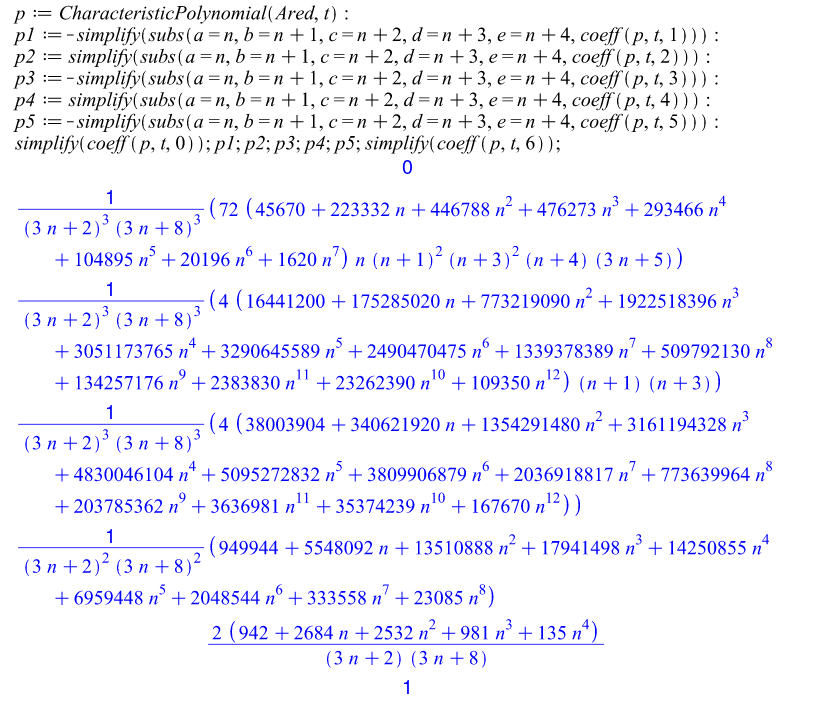
Figure 5: Coefficients of $\chi_{n}(t)=\det(t{\rm{Id}}_{6}-A_{\rm{red}})$, normalized case

The only modification of the above code in the non-normalized case is to set the variables eminus and eplus equal to $0$. The coefficients of $\chi_{n}(t)$ for $a=n,b=n+1,c=n+2,d=n+3,e=n+4$ are given in Figure 6. Again, all coefficients of $p_{j}(n)$, $j=1,2,3,4,5$, are non-negative.

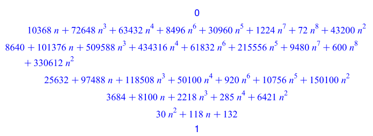
Figure 6: Coefficients of $\chi_{n}(t)=\det(t{\rm{Id}}_{6}-A_{\rm{red}})$, non-normalized case

Appendix B Maple Calculations for Theorems 4.3 and 4.4

For the Maple calculations needed for the proofs of these theorems, the code of Figure 4 is used again, followed by the code in Figure 7 (in the normalized case). The reduced matrices $A_{\rm{red}}$ are here of dimension $5$ and $3$, respectively, and they can be extracted from the original $6\times 6$ matrix as submatrices with specific choices for $a,b,c,d,e$. The crucial observation here is that the coefficients of the respective characteristic polynomials of degree $5$ and $3$ are alternating, guaranteeing that all non-zero roots are strictly positive.

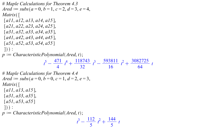
Figure 7: Calculation of $\chi(t)=\det(t{\rm{Id}}-A_{\rm{red}})$ for Theorems 4.3 amd 4.4, normalized case

As before, the non-normalized case is treated analogously with the small modification to set the variables eminus and eplus equal to $0$. This leads again to characteristic polynomials with alternating coefficients, given in the proofs of the theorems as

$$\chi(t)=t^{5}-132t^{4}+3684t^{3}-25632t^{2}+8640t$$

and

$$\chi(t)=t^{3}-44t^{2}+72t.$$

Appendix C Maple Calculations for Theorem 4.6

Using the information about $(A_{ij}(\delta,n))$ in the proof of Theorem 4.6, the Maple code to calculate the relevant polynomial $p_{1}(\delta,n)$ is given in Figure 8.

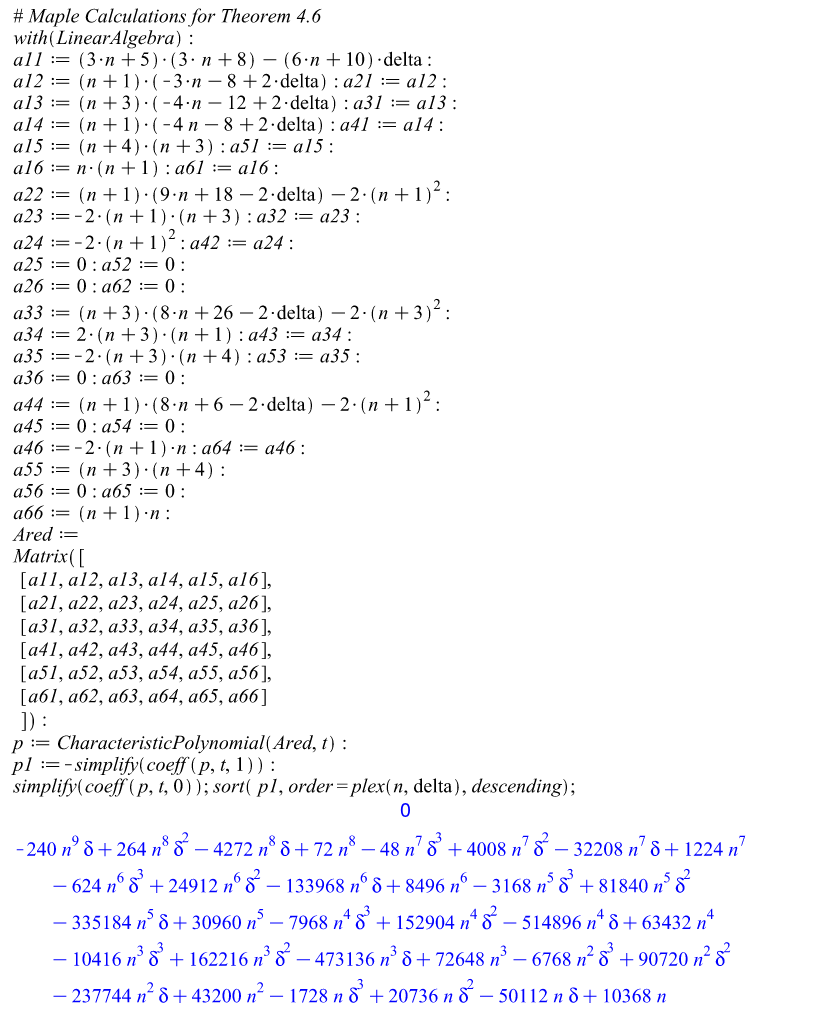
Figure 8: Calculation of $p_{1}(\delta,n)$ in the proof of Theorem 4.6

References

- [1] F. Bauer, M. Keller, and R. K. Wojciechowski, Cheeger inequalities for unbounded graph Laplacians, J. Eur. Math. Soc. (JEMS), 17(2):259–271, 2015.
- [2] D. Bakry and M. Émery, Diffusions hypercontractives, in Séminaire de probabilités, XIX, 1983/84, Lecture Notes in Math. 1123, 117–206, Springer, Berlin, 1985.
- [3] D. Bourne, D. Cushing, S. Liu, F. Münch, and N. Peyerimhoff, Ollivier-Ricci idleness functions of graphs, arXiv:1704.04398, (2016).
- [4] J. Breuer and M. Keller, Spectral analysis of certain spherically homogeneous graphs, Oper. Matrices, 7(4):825–847, 2013.
- [5] R. Brooks, A relation between growth and the spectrum of the Laplacian, Math. Z., 178(4):501–508, 1981.
- [6] D. Cushing, R. Kangaslampi, V. Lipläinen, S. Liu, and G. W. Stagg, The Graph Curvature Calculator and the curvatures of cubic graphs, arxiv:1712.03033, (2017).
- [7] D. Cushing, S. Liu, and N. Peyerimhoff, Bakry-Émery curvature functions of graphs, arXiv: 1606.01496, (2016).
- [8] J. Dodziuk and L. Karp, Spectral and function theory for combinatorial Laplacians, in Geometry of random motion (Ithaca, N.Y., 1987), Contemp. Math. 73, 25–40, Amer. Math. Soc., Providence, RI, 1988.
- [9] J. Dodziuk and V. Mathai, Kato’s inequality and asymptotic spectral properties for discrete magnetic Laplacians In The ubiquitous heat kernel, in The ubiquitous heat kernel, Contemp. Math. 398, 69–81, Amer. Math. Soc., Providence, RI, 2006.
- [10] R. L. Frank, D. Lenz, and D. Wingert, Intrinsic metrics for non-local symmetric Dirichlet forms and applications to spectral theory. J. Funct. Anal., 266(8):4765–4808, 2014.
- [11] M. Folz, Volume growth and stochastic completeness of graphs, Trans. Amer. Math. Soc., 366(4):2089–2119, 2014.
- [12] A. Grigor’yan, X. Huang, and J. Masamune’ On stochastic completeness of jump processes, Math. Z., 271(3- 4):1211–1239, 2012.
- [13] A. Grigor’yan, Analytic and geometric background of re- currence and non-explosion of the Brownian motion on Riemannian manifolds, Bull. Amer. Math. Soc. (N.S.), 36(2):135–249, 1999.
- [14] S. Golénia and Ch. Schumacher, The problem of deficiency indices for discrete Schrödinger operators on locally finite graphs, J. Math. Phys., 52(6), 2011.
- [15] S. Golénia and Ch. Schumacher, Comment on ’The problem of deficiency indices for discrete Schrödinger operators on locally finite graphs’, J. Math. Phys., 54(6), 2013.
- [16] S. Haeseler, M. Keller, and R. K. Wojciechowski, Volume growth and bounds for the essential spectrum for Dirichlet forms, J. Lond. Math. Soc. (2), 88(3):883–898, 2013.
- [17] B. Hua and F. Münch, Ricci curvature on birth-death processes, arXiv:1712.01494, (2017).
- [18] X. Huang, A note on the volume growth criterion for stochastic completeness of weighted graphs, Potential Anal., 40(2):117–142, 2014.
- [19] M. Keller, D. Lenz, and R. K. Wojciechowski, Volume growth, spectrum and stochastic completeness of infinite graphs, Math. Z., 274(3-4):905–932, 2013.
- [20] Y. Lin, L. Lu, and S.-T. Yau, Ricci curvature of graphs, Tohoku Math. J. (2), 63(4):605–627, 2011.
- [21] S. Liu, F. Münch, and N. Peyerimhoff, Bakry-Émery curvature and diameter bounds on graphs, arXiv:1608.07778, (2016).
- [22] F. Münch and R. K. Wojciechowski, Ollivier Ricci curvature for general graph Laplacians: Heat equation, Laplacian comparison, non-explosion and diameter bounds, arXiv:1712.00875, (2017).
- [23] Y. Ollivier, Ricci curvature of Markov chains on metric spaces, J. Funct. Anal., 256(3):810–864, 2009.
- [24] A. Weber, Analysis of the physical Laplacian and the heat flow on a locally finite graph, J. Math. Anal. Appl., 370(1):146–158, 2010.
- [25] R. K. Wojciechowski, Stochastically incomplete manifolds and graphs, in Random walks, boundaries and spectra, Progr. Probab. 64, 163–179, Birkhäuser/Springer Basel AG, Basel, 2011.