Safeguarding Millimeter Wave Communications Against Randomly Located Eavesdroppers

Abstract

Millimeter wave offers a sensible solution to the capacity crunch faced by 5G wireless communications. This paper comprehensively studies physical layer security in a multi-input single-output (MISO) millimeter wave system where multiple single-antenna eavesdroppers are randomly located. Concerning the specific propagation characteristics of millimeter wave, we investigate two secure transmission schemes, namely maximum ratio transmitting (MRT) beamforming and artificial noise (AN) beamforming. Specifically, we first derive closed-form expressions of the connection probability for both schemes. We then analyze the secrecy outage probability (SOP) in both non-colluding eavesdroppers and colluding eavesdroppers scenarios. Also, we maximize the secrecy throughput under a SOP constraint, and obtain optimal transmission parameters, especially the power allocation between AN and the information signal for AN beamforming. Numerical results are provided to verify our theoretical analysis. We observe that the density of eavesdroppers, the spatially resolvable paths of the destination and eavesdroppers all contribute to the secrecy performance and the parameter design of millimeter wave systems.

I Introduction

Driven by an increasing number of smart devices and wireless data applications, an explosive growth of demand for spectrum in wireless communications appears during the past years. Exploiting millimeter wave becomes a promising approach for providing plentiful spectrum resources to improve the system capacity [LABEL:r1], [LABEL:r2]. Following this trend, the study on millimeter wave communications has attracted great research affords. Millimeter wave channel modeling [LABEL:r3], [LABEL:r5], beamforming schemes [LABEL:r6]-[LABEL:r10] and network performance [LABEL:r41], [LABEL:r42] have been investigated intensively in the past few years. It becomes a promising candidate for the 5G cellular system.

Given the open feature of the wireless channels, security is a significant concern when designing wireless transmission schemes. Physical layer security has become a popular way to improve the secrecy performance of wireless communication systems by utilizing wireless channel characteristics [LABEL:r11]-[LABEL:r12]. Thanks to the application of multi-antenna techniques, physical layer security is greatly enhanced in [LABEL:r13], [LABEL:r15]. With multiple antennas, the transmitter can use transmit beamforming either to enhance the legitimate user’s channel, i.e., maximum ratio transmitting (MRT) beamforming [LABEL:r16], or to deteriorate eavesdroppers’ channels by emitting artificial noise (AN), i.e., AN beamforming [LABEL:r19], [LABEL:r21]. Also, transmit antenna selection technique can be exploited as an effective approach to improve the quality of the legitimate user’s channel [LABEL:r47]. When designing secure transmission schemes, reducing secrecy outage probability (SOP) [LABEL:r16], [LABEL:r47] and increasing secrecy throughput [LABEL:r21] are two significant goals.

In wiretap scenarios, eavesdroppers are always passive and their locations are hard to acquire in practice. To model the unknown locations of potential eavesdroppers, stochastic geometry theory has provided a powerful tool recently, with which eavesdroppers’ positions can be represented by a spatial distribution such as a Poisson point process (PPP) [LABEL:r22]-[LABEL:r241]. This makes the secure transmission scheme design and secrecy performance evaluation possible in the wireless systems with potentially unknown eavesdroppers.

We should point out that, the wireless channel significantly influences the design and analysis of physical layer security, and the millimeter wave channel is truly different from the traditional microwave channel which has rich scattering. Based on the measurements conducted in New York City, the ray cluster channel model, constituted by several clusters of propagation paths, is built for millimeter wave systems [LABEL:r5]. This model is further adopted in [LABEL:r6]-[LABEL:r9] to design and analyze millimeter wave beamforming schemes. Therefore, the major concern for the implementation of physical layer security in millimeter wave communication systems is the specific propagation characteristics of millimeter wave, which can be described as follows. Firstly, due to the sparse multipaths and scattering of the millimeter wave propagation environment, traditional statistically independent fading distributions are no longer suitable to model the millimeter wave channel. Channels in the millimeter wave band are correlated fading rather than independent and identically distributed (i.i.d.) Rayleigh. Secondly, the small carrier wavelength of millimeter wave enables the realization of large antenna arrays, which can produce extremely high beamforming gain and directionality [LABEL:r26]. This helps to improve the secrecy performance of millimeter wave transmission [LABEL:r29].

Driven by the new propagation features, studies on secure transmissions in millimeter wave systems spring up, both in point-to-point transmissions [LABEL:r28]-[LABEL:r39] and networks [LABEL:r36]-[LABEL:r43]. Specifically, for the point-to-point millimeter wave systems, switched array techniques are utilized in [LABEL:r28], [LABEL:r35], where a subset of transmit antennas are randomly selected to emit signals with every symbol period. This results in a clear constellation in the legitimate user’s direction and a high symbol error rate in undesired directions. This method that needs only a single RF chain is easy to implement in millimeter wave systems. However, the switching speed to be matched at per-symbol rate leads to a huge system overhead, and the antenna sparsity caused by switching makes the secure transmission vulnerable to attacking [LABEL:r40]. Hybrid beamforming design for millimeter wave systems to resist eavesdropping is studied in [LABEL:r44], [LABEL:r45]. Furthermore, in our previous work [LABEL:r46]-[LABEL:r39], we design beamforming schemes and analyze secrecy performance for the millimeter wave system which contains only one eavesdropper. For the scope of millimeter wave networks, the authors in [LABEL:r36]-[LABEL:r43] analyze the secrecy performance of cellular or Ad hoc networks under the stochastic geometry framework. Both the noise-limited and AN-assisted cellular networks are considered in [LABEL:r36]. The tradeoff between the connection outage probability and secrecy outage probability is investigated for a microwave and millimeter wave hybrid cellular network in [LABEL:r37]. The impact of random blockages and antenna gain on the secrecy performance of Ad hoc networks is analyzed in [LABEL:r43]. These three works focus on the network-wide performance analysis, and the beam pattern is approximated by a sectored antenna model for mathematical tractability.

In all the aforementioned studies, they either do not consider multipath transmission, or do not investigate the effect of multiple randomly distributed eavesdroppers. To the best of our knowledge, no previous work has provided secure transmission schemes and comprehensive secrecy performance analysis under a more practical ray cluster channel model that characterizes multipath propagation for a millimeter wave system with the stochastic geometry framework. So far, how to safeguard the point-to-point millimeter wave system against randomly located eavesdroppers under a more practical millimeter wave channel model is still unknown, which motivates our work.

I-A Our Work and Contributions

In this paper, we study physical layer security in a multi-input single-output (MISO) millimeter wave system considering multipath propagation under a stochastic geometry framework, where the locations of multiple single-antenna eavesdroppers are modeled as a homogeneous PPP. Connection probability, SOP and secrecy throughput are studied to evaluate the secrecy performance of the transmission schemes. Our contributions are summarized as follows:

1) In the presence of multiple randomly located eavesdroppers, we investigate two transmission schemes, namely MRT beamforming and AN beamforming, under the discrete angular domain channel model which characterized by multiple spatially resolvable paths. We obtain the probability distribution function (PDF) for the number of overlapped common channel paths between the destination and an arbitrary eavesdropper to facilitate the secrecy performance analysis.

2) We derive the closed-form connection probability for both transmission schemes and evaluate the impact of the number of destination’s resolvable paths on the connection. Then we obtain the closed-form expressions of SOP for the non-colluding eavesdroppers scenario and the accurate approximation of SOP for the colluding eavesdroppers scenario. In addition, we maximize the secrecy throughput for both schemes, and derive the optimal power allocation between AN and the information signal for the AN scheme. we observe that more power should be allocated to AN in the dense eavesdroppers scenario or in the situation where the number of the destination’s resolvable paths or that of the eavesdropper’s resolvable paths is large.

3) We reveal that AN beamforming has a better secrecy performance than MRT beamforming when the number of the eavesdropper’s resolvable paths is large, the density of eavesdroppers is large or the transmit power is high. Otherwise, MRT beamforming as a simple method shows its superiority. Furthermore, we find that the decrease of the number of the destination’s resolvable paths is beneficial for improving the secrecy performance in both beamforming schemes, while the impact of the number of the eavesdropper’s resolvable paths on the secrecy throughput are different between two schemes.

I-B Organization and Notations

This paper is organized as follows. In Section II, we build the channel model, analyze spatially resolvable paths, and describe performance metrics. In Section III, we propose two secure transmission schemes against randomly located eavesdroppers. In Sections IV and LABEL:s4, we analyze the connection probability, the SOP and the secrecy throughput for both schemes. In Section LABEL:s6, we provide numerical results to verify our theoretical analysis. In Section LABEL:s7, we conclude our paper.

We use the following notations in this paper: bold uppercase (lowercase) letters denote matrices (vectors). $(\cdot)^{*}$, $(\cdot)^{T}$, $(\cdot)^{H}$, $|\cdot|$, $\|\cdot\|$, $\mathbb{P\{\cdot\}}$ and $\mathbb{E}_{A}\{\cdot\}$ denote conjugate, transpose, conjugate transpose, absolute value, Euclidean norm, probability, and mathematical expectation with respect to A, respectively. $\mathcal{CN}(\mu,\sigma^{2})$, $\operatorname{Exp}(\lambda)$ and $\operatorname{Gamma}(N,\lambda)$ denote circularly symmetric complex Gaussian distribution with mean $\mu$ and variance $\sigma^{2}$, exponential distribution with parameter $\lambda$, and gamma distribution with parameters $N$ and $\lambda$, respectively. $\mathbb{C}^{M\times N}$ denotes the space of all $M\times N$ matrices with complex-valued elements. $\mathbb{Z}^{+}$ denotes positive integer domain. $\operatorname{log}(\cdot)$, $\operatorname{lg}(\cdot)$ and $\operatorname{ln}(\cdot)$ denote base-2, base-10 and natural logarithms, respectively. $f_{u}(\cdot)$, $F_{u}(\cdot)$ and $F_{u}^{-1}(\cdot)$ denote the PDF, cumulative distribution function (CDF) of $u$ and inverse function of $F_{u}(\cdot)$, respectively. The intersection, union and difference between two sets $\Omega_{1}$ and $\Omega_{2}$ are denoted by $\Omega_{1}\cap\Omega_{2}$, $\Omega_{1}\cup\Omega_{2}$ and $\Omega_{1}\backslash\Omega_{2}$, respectively. $\operatorname{E}_{i}(-x)=\int_{x}^{\infty}\frac{e^{-t}}{t}dt$ with $x>0$.

II System Model

We consider a millimeter wave system where a transmitter communicates with a destination while randomly located eavesdroppers attempt to intercept the information. The transmitter is equipped with $N_{t}$ antennas, the destination and eavesdroppers are all equipped with single antenna. Without loss of generality, we assume the transmitter is located at the origin and the destination is located at coordinate ($r_{d}$, 0). As shown in Fig. 1(a), eavesdroppers are located according to a homogeneous PPP $\Phi_{e}$ of density $\lambda$ on the 2-D plane with the $k^{th}$ eavesdropper having a distance $r_{k}$ from the transmitter.

II-A Discrete Angular Domain Channel Model

Due to the sparse characteristics of the millimeter wave propagation environment, millimeter wave channels can be described by a ray cluster based spatial channel model [LABEL:r5]-[LABEL:r9]. The channel is assumed to be a sum of the contributions of $N_{c}$ clusters with $N_{r}$ paths in each cluster and can be formulated as $\mathbf{h}=\sqrt{\frac{\beta}{N_{c}N_{r}}}\sum_{l_{c}}\sum_{l_{r}}g_{l_{c},l_{r}}\mathbf{a}(\Theta_{l_{c},l_{r}})^{H}$, where $\beta$ is the average path loss between the transmitter and the receiver, $g_{l_{c},l_{r}}$ is the complex gain of the $l_{r}^{th}$ path in the $l_{c}^{th}$ cluster, $\mathbf{a}(\Theta_{l_{c},l_{r}})$ is the normalized array response at the azimuth angle of departure (AOD) of $\theta_{l_{c},l_{r}}$, and $\Theta_{l_{c},l_{r}}\triangleq\sin(\theta_{l_{c},l_{r}})$. When a uniform linear array (ULA) is adopted, the normalized array response can be described as $\mathbf{a}(\Theta)=\frac{1}{\sqrt{N_{t}}}\left[1,e^{-j\frac{2\pi d}{\lambda}\Theta},e^{-j2\frac{2\pi d}{\lambda}\Theta},\cdots,e^{-j(N_{t}-1)\frac{2\pi d}{\lambda}\Theta}\right]^{T}$, where $d$ is the antenna spacing, $\lambda$ is the wavelength, and generally $d=\frac{\lambda}{2}$.

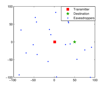
(a) Locations of randomly distributed eavesdroppers

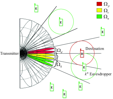
(b) Description of spatially resolvable paths

Figure 1: Millimeter wave system model with stochastic geometry framework.

Based on the ray cluster model, in order to conduct the theoretical analysis of the transmission schemes, the millimeter wave channel is modeled as a discrete angular domain channel model in existing literature [LABEL:r3], [LABEL:r31], [LABEL:r32] and our previous work [LABEL:r46], which can be described as

$$\mathbf{h}=\sqrt{\frac{1}{L}}r^{-\frac{\alpha}{2}}\mathbf{g}\mathbf{U}^{H},$$ (1)

where $\mathbf{g}=[g_{1},g_{2},\cdots,g_{Nt}]$ is the complex gain vector, $r^{-\frac{\alpha}{2}}$ is the average path loss, $r$ is the distance between the transmitter and the receiver, $\mathbf{U}\triangleq[\mathbf{a}(\Psi_{1}),\mathbf{a}(\Psi_{2}),\cdots,\mathbf{a}(\Psi_{Nt})]$ is the spatially orthogonal basis with $\Psi_{i}\triangleq\frac{1}{M}(i-1-\frac{N_{t}-1}{2})$ and $M=N_{t}\frac{d}{\lambda}$. This model is based on the principle that every aperture-limited system has a finite angular resolution [LABEL:r31]. Since paths with $\Theta$ differing by less than $\frac{1}{M}$ are not resolvable by the array, the angular domain can be sampled at a fixed spacing $\frac{1}{M}$ and represented by the spatially orthogonal basis $\mathbf{U}$. Experimental results in [LABEL:r5], [LABEL:r30] show that the millimeter wave channel most likely contains only one cluster where the overwhelming proportion of transmit power is concentrated on. Therefore, we assume that signals are transmitted through one cluster and all the AODs of paths are distributed within the angular range $[\theta_{\operatorname{min}},\theta_{\operatorname{max}}]$. If $\Psi_{i}\in\left[\operatorname{sin}(\theta_{\operatorname{min}}),\operatorname{sin}(\theta_{\operatorname{max}})\right]$, the $i^{th}$ column of $\mathbf{U}$ (the $i^{th}$ orthogonal basis vector) represents a spatially resolvable path and we assume that the $i^{th}$ complex gain $g_{i}$ is a complex Gaussian coefficient with $g_{i}\sim\mathcal{CN}(0,1)$; otherwise, $g_{i}=0$ [LABEL:r5], [LABEL:r26], [LABEL:r46]. $L$ is defined as the number of spatially resolvable paths with $L<N_{t}$. Then the channels of the destination and the $k^{th}$ eavesdropper can be described as $\mathbf{h}_{d}=\sqrt{\frac{1}{L_{d}}}r_{d}^{-\frac{\alpha}{2}}\mathbf{g}_{d}\mathbf{U}^{H}$ and $\mathbf{h}_{k}=\sqrt{\frac{1}{L_{e}}}r_{k}^{-\frac{\alpha}{2}}\mathbf{g}_{k}\mathbf{U}^{H}$, where $L_{d}$ and $L_{e}$ are the numbers of the destination’s and each eavesdropper’s resolvable paths, respectively.

We assume the AODs of all the destination’s paths and those of the $k^{th}$ eavesdropper’s paths are distributed within the angular range $[\theta_{d,\operatorname{min}},\theta_{d,\operatorname{max}}]$ and $[\theta_{k,\operatorname{min}},\theta_{k,\operatorname{max}}]$ respectively. As shown in Fig. 1(b), we define the set $\Omega_{d}\triangleq\{I_{d,i}|I_{d,i}\in\mathbb{Z}^{+},\Psi_{I_{d,i}}\in[\operatorname{sin}(\theta_{d,\operatorname{min}}),\operatorname{sin}(\theta_{d,\operatorname{max}})],I_{d,1}<I_{d,2}<\cdots<I_{d,L_{d}}\}$, where $I_{d,i}$ is an index of the orthogonal basis vector which represents a destination’s spatially resolvable path. Define the set $\Omega_{k}\triangleq\{I_{k,i}|I_{k,i}\in\mathbb{Z}^{+},\Psi_{I_{k,i}}\in[\operatorname{sin}(\theta_{k,\operatorname{min}}),\operatorname{sin}(\theta_{k,\operatorname{max}})],I_{k,1}<I_{k,2}<\cdots<I_{k,L_{e}}\}$, where $I_{k,i}$ is an index of the orthogonal basis vector which represents a resolvable path of the $k^{th}$ eavesdropper. Define $\Omega=\{1,2,\cdots,N_{t}\}$, $\Omega_{a}\triangleq\overline{\Omega}_{d}=\Omega\backslash\Omega_{d}$, $\Omega_{c,k}\triangleq\Omega_{d}\cap\Omega_{k}$ and $\Omega_{p,k}\triangleq\Omega_{d}\backslash\Omega_{c,k}$, $\Omega_{n,k}\triangleq\Omega_{k}\backslash\Omega_{c,k}$. Also, we denote $L_{c,k}$ as the number of the overlapped common paths between the destination and the $k^{th}$ eavesdropper. For notational brevity, we omit $k$ from $L_{c,k}$, $\Omega_{c,k}$, $\Omega_{p,k}$ and $\Omega_{n,k}$, and treat $L_{c}$, $\Omega_{c}$, $\Omega_{p}$ and $\Omega_{n}$ as functions of $k$ by default. We define the function $\mathcal{S}(\mathbf{B},\Omega_{s})$ to generate a matrix whose columns are selected from $\mathbf{B}$, and $\Omega_{s}$ contains all the selected columns’ indexes. Define $\mathbf{g}_{\varrho\nu}\triangleq\mathcal{S}(\mathbf{g}_{\varrho},\Omega_{\nu})\in\mathbb{C}^{1\times L_{\nu}}$, where $\varrho\in\{d,k\}$, $\nu\in\{c,p,n,a\}$, and $L_{\nu}$ is the cardinality of $\Omega_{\nu}$.

We assume that the instantaneous channel state information (CSI) of the destination is perfectly known at the transmitter [LABEL:r19], [LABEL:r21]. Since eavesdroppers passively receive signals, their instantaneous CSIs are unknown, whereas the distribution of $\mathbf{g}_{k}$ is available.

II-B Spatially Resolvable Paths

Unlike the traditional wireless channels with rich scattering, the millimeter wave channel involves a limited angular coverage which is represented by the directions of propagation paths. As we have demonstrated in [LABEL:r46], the secrecy performance of the millimeter wave system is dramatically influenced by $L_{c}$, which is the number of the overlapped common paths between the eavesdropper’s and the destination’s spatially resolvable paths. When $L_{c}$ becomes larger, the correlation between the channel of the destination and that of the eavesdropper is larger. More confidential information is leaked to the eavesdropper so that the secrecy performance will be poorer. However, under the stochastic geometry framework, it is hard to get the exact value of $L_{c}$ due to the randomness of eavesdroppers’ locations and the lack of eavesdroppers’ CSIs. Fortunately, we derive the PDF of $L_{c}$ in the following lemma, which will be extensively used in subsequent sections.

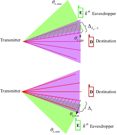
(a) $L_{c}=1$

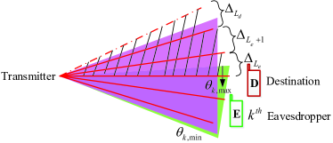
(b) $L_{c}=L_{e}$($L_{d}=5,L_{e}=3$)

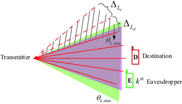
(c) $L_{c}=L_{d}$($L_{d}=5,L_{e}=6$)

Figure 2: Distribution for the number of the overlapped common paths between the destination and the $k^{th}$ eavesdropper. The pink area shows the angular range $[\theta_{d,\operatorname{min}},\theta_{d,\operatorname{max}}]$ where AODs of the destination’s paths are distributed in, and the green area shows the angular range $[\theta_{k,\operatorname{min}},\theta_{k,\operatorname{max}}]$ where AODs of the $k^{th}$ eavesdropper’s paths are distributed in. Red solid lines are the spatially resolvable paths of the destination. Each red dashed line represents an angle in $\mathbf{U}$ but not the spatially resolvable path of the destination. (a) describes the situation that $L_{c}=1$, which is similar as all the situations when $L_{c}<L_{l}$. (b) and (c) describe the situation that $L_{c}=L_{l}$ with $L_{d}>L_{e}$ and $L_{d}<L_{e}$ respectively.

Lemma 1

The PDF of $L_{c}$ can be given by

$$p(L_{c})=\left\{\begin{aligned} &\frac{\sum_{i=L_{l}}^{L_{u}}\omega_{i}}{\pi},\ \ \ \ \ L_{c}=L_{l},\\ &\frac{2\omega_{L_{c}}}{\pi},\ \ \ \ \ \ \ \ \ \ L_{c}=1,2,\cdots,L_{l}-1,\\ &1-\sum_{i=1}^{L_{l}}p(i),\ \ \ L_{c}=0,\\ \end{aligned}\right.$$ (2)

where $\omega_{i}\triangleq\arcsin\left(\Psi_{\frac{N_{t}-L_{d}}{2}+i+1}\right)-\arcsin\left(\Psi_{\frac{N_{t}-L_{d}}{2}+i}\right)$, $L_{l}\triangleq\operatorname{min}\{L_{d},L_{e}\}$ and $L_{u}\triangleq\operatorname{max}\{L_{d},L_{e}\}$.

Proof 1

Eavesdroppers are located according to a homogeneous PPP so that the angles of eavesdroppers’ locations are uniformly distributed within the range $[-\frac{\pi}{2},\frac{\pi}{2}]$. In order to get the probability of $L_{c}=m$, $m\in\{0,1,\cdots,\min\{L_{d},L_{e}\}\}$, we need to know the angular range $\Upsilon_{m}$ which satisfies that, the destination and the $k^{th}$ eavesdropper will have $m$ overlapped common resolvable paths when the $k^{th}$ eavesdropper is located in $\Upsilon_{m}$. In other words, $[\theta_{k,\operatorname{min}},\theta_{k,\operatorname{max}}]$ should cover $m$ destination’s spatially resolvable paths, where $[\theta_{k,\operatorname{min}},\theta_{k,\operatorname{max}}]$ is the angular range where AODs of the $k^{th}$ eavesdropper’ paths are distributed in as discussed in the last subsection. Then we can obtain the probability $p(m)=\frac{\mathcal{W}(\Upsilon_{m})}{\pi}$, where $\mathcal{W}(\cdot)$ denotes the width of an angular range. With this idea in mind, we move the $k^{th}$ eavesdropper to find out the angular range $\Upsilon_{m}$ as shown in Fig. 2.

Since the destination is located at ($r_{d}$, 0) and with $L_{d}$ resolvable paths, we have $\Omega_{d}=\noindent\{\frac{N_{t}-L_{d}}{2}+1,\frac{N_{t}-L_{d}}{2}+2,\cdots,\frac{N_{t}+L_{d}}{2}-1,\frac{N_{t}+L_{d}}{2}\}$ where $\Omega_{d,i}=\frac{N_{t}-L_{d}}{2}+i$. Define the angular range $\Delta_{i}\triangleq$

$\left[\operatorname{arcsin}\left(\Psi_{\frac{N_{t}-L_{d}}{2}+i}\right),\operatorname{arcsin}\left(\Psi_{\frac{N_{t}-L_{d}}{2}+i+1}\right)\right]$, and the width $\omega_{i}\triangleq\mathcal{W}(\Delta_{i})=\arcsin\left(\Psi_{\frac{N_{t}-L_{d}}{2}+i+1}\right)-\arcsin\left(\Psi_{\frac{N_{t}-L_{d}}{2}+i}\right)$. We find that $\Delta_{i}$ describes the angular range between the $i^{th}$ and the $(i+1)^{th}$ spatially resolvable paths of the destination when $1\leq i\leq L_{d}-1$. Due to the symmetry of the sine function and the definition of $\Psi_{i}$, we have $\omega_{i}=\omega_{L_{d}-i}$.

As shown in Fig. 2(a), if $\theta_{k,\operatorname{max}}$ is located within $\Delta_{1}$ or $\theta_{k,\operatorname{min}}$ is located within $\Delta_{L_{d}-1}$, we have $L_{c}=1$. Thus we derive the PDF of $L_{c}=1$, which is $p(1)=\frac{\omega_{1}+\omega_{(L_{d}-1)}}{\pi}=\frac{2\omega_{1}}{\pi}$. Then we analyze two different cases $L_{d}\geq L_{e}$ and $L_{d}<L_{e}$.

1) $L_{d}\geq L_{e}$

In this case, $0\leq L_{c}\leq L_{e}$. From the analysis of $L_{c}=1$ given above, we derive the PDFs $p(L_{c})=\frac{2\omega_{L_{c}}}{\pi},L_{c}=1,2,\cdots,L_{e}-1$ by analogy. The situation when $L_{c}=L_{e}$ is special. As shown in Fig. 2(b), when $\theta_{k,\max}\in\Delta_{L_{e}}\cup\Delta_{L_{e}+1}\cup\cdots\cup\Delta_{L_{d}}$, $L_{c}=L_{e}$, hence we have $p(L_{c})=\frac{\sum_{i=L_{e}}^{L_{d}}\omega_{i}}{\pi}$.

2) $L_{d}<L_{e}$

In this case, $0\leq L_{c}\leq L_{d}$, and we derive the PDFs $p(L_{c})=\frac{2\omega_{L_{c}}}{\pi},L_{c}=1,2,\cdots,L_{d}-1$. As shown in Fig. 2(c), when $\theta_{k,\max}\in\Delta_{L_{d}}\cup\Delta_{L_{d}+1}\cup\cdots\cup\Delta_{L_{e}}$, $L_{c}=L_{d}$, hence we have $p(L_{c})=\frac{\sum_{i=L_{d}}^{L_{e}}\omega_{i}}{\pi}$.

Combining the above two cases completes the proof.

II-C Wiretap Encoding Scheme and Performance Metrics

We consider both non-colluding eavesdroppers and colluding eavesdroppers scenarios. In non-colluding eavesdroppers scenario, each eavesdropper individually decodes confidential messages and the equivalent signal-to-interference-plus-noise ratio (SINR) of the wiretap channel can be expressed as $\xi_{e}=\operatorname{max}_{e_{k}\in\Phi_{e}}\xi_{k}$, where $\xi_{k}$ is the received SINR of the $k^{th}$ eavesdropper. In colluding eavesdropper scenario, eavesdroppers jointly decode confidential messages with maximum ratio combining reception and $\xi_{e}=\sum_{e_{k}\in\Phi_{e}}\xi_{k}$. Then the capacities of the destination’s channel and the wiretap channel are $C_{d}=\operatorname{log}(1+\xi_{d})$ and $C_{e}=\operatorname{log}(1+\xi_{e})$. Adopting the well-known Wyner’s wiretap encoding scheme, we denote the codeword rate and secrecy rate as $R_{t}$ and $R_{s}$. In addition, we define $R_{e}\triangleq R_{t}-R_{s}$ as the rate redundancy to resist the interception. We analyze the following metrics to evaluate the secrecy performance of transmission schemes.

Connection probability: Only if $C_{d}>R_{t}$, the destination is able to decode the confidential message correctly. This corresponds to a reliable connection event. We define connection probability as

$$\mathcal{P}_{c}=\mathbb{P}\{C_{d}>R_{t}\}.$$ (3)

Secrecy outage probability: If $C_{e}>R_{e}$, perfect secrecy is broken and a secrecy outage occurs. We adopt an on-off transmission scheme proposed in [LABEL:r21], where the transmitter decides whether to transmit or not based on the instantaneous CSI of the destination. Throughout the paper, for notational brevity, we define $\mu\triangleq\|\mathbf{g}_{d}\|^{2}$ as the overall channel gain of the destination and $\delta$ as the transmission threshold. Since the channel gain $\mu$ varies from time to time, the transmitter emits signals only when $\mu>\delta$; otherwise, the transmission suspends. The SOP is defined as

$$\mathcal{P}_{so}=\mathbb{P}\{C_{e}>R_{t}-R_{s}|\mu\},\ \forall\mu>\delta.$$ (4)

Secrecy throughput: Secrecy throughput is defined as the effective average transmission rate of the confidential message, which is formulated as

$$\tau=\mathbb{E}_{\mu}\left[R_{s}(\mu)\right],$$ (5)

where $R_{s}(\mu)=0$ for $\mu\leq\delta$.

III Transmission Schemes

In this section, we propose two transmission schemes, namely MRT beamforming and AN beamforming, to resist overhearing of multiple randomly located eavesdroppers.

III-A MRT Beamforming

By exploiting MRT beamforming, the signals received at the destination and the $k^{th}$ eavesdropper are $y_{d}^{MRT}=\sqrt{P}\mathbf{h}_{d}\mathbf{w}_{1}s+n_{d}$ and $y_{k}^{MRT}=\sqrt{P}\mathbf{h}_{k}\mathbf{w}_{1}s+n_{k}$, where $\mathbf{w}_{1}=\mathbf{h}_{d}^{H}/\|\mathbf{h}_{d}\|$ is the beamforming vector, $P$ is the total transmit power, $s$ is the information bearing signal with $\mathbb{E}[|s|^{2}]=1$, $n_{d}$ and $n_{k}$ are i.i.d. additive white Gaussian noise with $n_{d}\sim\mathcal{CN}(0,\sigma_{n}^{2})$ and $n_{k}\sim\mathcal{CN}(0,\sigma_{n}^{2})$. We define $\mu_{c,k}\triangleq\|\mathbf{g}_{dc}\|^{2}$ and $\mu_{p,k}\triangleq\|\mathbf{g}_{dp}\|^{2}$ as the destination’s channel gain of the common paths and the non-common paths with the $k^{th}$ eavesdropper. For notational brevity, we omit $k$ from $\mu_{c,k}$ and $\mu_{p,k}$, and treat them as functions of $k$ by default. We easily find that $\mu=\mu_{c}+\mu_{p}$. Then the SNRs of the destination and the $k^{th}$ eavesdropper can be respectively described as

$$\xi_{d}^{MRT}=\frac{Pr_{d}^{-\alpha}}{\sigma_{n}^{2}L_{d}}\|\mathbf{g}_{d}\mathbf{U}^{H}\|^{2}=c\mu r_{d}^{-\alpha},$$ (6)

$$\xi_{k}^{MRT}=\frac{Pr_{k}^{-\alpha}|\mathbf{g}_{k}\mathbf{U}^{H}\mathbf{U}\mathbf{g}_{d}^{H}|^{2}}{\sigma_{n}^{2}L_{e}\|\mathbf{g}_{d}\mathbf{U}^{H}\|^{2}}=\frac{a\mu_{c}r_{k}^{-\alpha}|\mathbf{g}_{kc}\frac{\mathbf{g}_{dc}^{H}}{\|\mathbf{g}_{dc}\|}|^{2}}{\mu}.$$ (7)

where $a\triangleq\frac{P}{L_{e}\sigma_{n}^{2}}$ and $c\triangleq\frac{P}{L_{d}\sigma_{n}^{2}}$. We find that $g_{k,i}g_{d,i}^{*}\neq 0$ only if $i\in\Omega_{d}\cap\Omega_{k}$, i.e., $i\in\Omega_{c}$. Thus we have $\mathbf{g}_{k}\mathbf{g}_{d}^{H}=\mathbf{g}_{kc}\mathbf{g}_{dc}^{H}$.

III-B AN Beamforming

Based on the CSI of the destination, we design the AN beamforming matrix as $\mathbf{W}_{2}=\mathcal{S}(\mathbf{U},\Omega_{a})$ to transmit AN to the null space of the destination’s channel. Since $\Omega_{a}=\Omega\backslash\Omega_{d}$, we have $\mathbf{h}_{d}\mathbf{W}_{2}=\mathbf{0}$, hence the destination is not influenced by AN. We observe that by leveraging the specific propagation characteristics of millimeter wave, we form the null space only through selecting some columns from $\mathbf{U}$, which is really simple to operate. Then signals received by the destination and the $k^{th}$ eavesdropper can be described as $y_{d}^{AN}=\sqrt{\eta P}\mathbf{h}_{d}\mathbf{w}_{1}s+\sqrt{\frac{(1-\eta)P}{N_{t}-L_{d}}}\mathbf{h}_{d}\mathbf{W}_{2}\mathbf{z}+n_{d}$ and $y_{k}^{AN}=\sqrt{\eta P}\mathbf{h}_{k}\mathbf{w}_{1}s+\sqrt{\frac{(1-\eta)P}{N_{t}-L_{d}}}\mathbf{h}_{k}\mathbf{W}_{2}\mathbf{z}+n_{k}$, where $\mathbf{z}\in\mathbb{C}^{(N_{t}-L_{d})\times 1}$ is the AN bearing signal with $\mathbb{E}[\mathbf{z}\mathbf{z}^{H}]=\mathbf{I}_{N_{t}-L_{d}}$, $\eta$ is the power allocation ratio of the information signal power to the total transmit power with $0\leq\eta\leq 1$. When $\eta=1$, AN beamforming is equavalent to MRT beamforming where information signal is transmitted with full power. The SINRs of the destination and the $k^{th}$ eavesdropper can be respectively formulated as

$$\xi_{d}^{AN}=\frac{\eta Pr_{d}^{-\alpha}}{\sigma_{n}^{2}L_{d}}\|\mathbf{g}_{d}\mathbf{U}^{H}\|^{2}=\eta c\mu r_{d}^{-\alpha},$$ (8)

$$\xi_{k}^{AN}=\frac{\frac{\eta Pr_{k}^{-\alpha}}{L_{e}\mu}|\mathbf{g}_{k}\mathbf{U}^{H}\mathbf{U}\mathbf{g}_{d}^{H}|^{2}}{\frac{(1-\eta)Pr_{k}^{-\alpha}}{(N_{t}-L_{d})L_{e}}\|\mathbf{g}_{k}\mathbf{U}^{H}\mathbf{W}_{2}\|^{2}+\sigma_{n}^{2}}$$

$$\ \ \ \ \ =\frac{\frac{\eta a\mu_{c}r_{k}^{-\alpha}}{\mu}|\mathbf{g}_{kc}\frac{\mathbf{g}_{dc}^{H}}{\|\mathbf{g}_{dc}\|}|^{2}}{\frac{(1-\eta)ar_{k}^{-\alpha}}{(N_{t}-L_{d})}\|\mathbf{g}_{kn}\|^{2}+1}.$$ (9)

By denoting $\mathbf{g}_{k}\mathbf{U}^{H}\mathbf{W}_{2}=\left[\chi_{1},\chi_{2},\cdots,\chi_{(N_{t}-L_{d})}\right]$, we have $\chi_{j}=\sum_{i=1}^{N_{t}}g_{k,i}\mathbf{a}(\Psi_{i})^{H}\mathbf{w}_{2,j}$. Since $\mathbf{W}_{2}=\mathcal{S}(\mathbf{U},\Omega_{a})$ and $\mathbf{U}$ is a unitary matrix, we get $\mathbf{g}_{k}\mathbf{U}^{H}\mathbf{W}_{2}=\mathbf{g}_{ka}$. Since $\Omega_{n}=\Omega_{k}\backslash\Omega_{c}$, by getting rid of those zero elements in $\mathbf{g}_{ka}$, we have $\|\mathbf{g}_{ka}\|=\|\mathbf{g}_{kn}\|$.

IV Secrecy Performance of MRT Beamforming

In this section, we analyze the secrecy performance in terms of the connection probability, the SOP and the secrecy throughput for MRT beamforming.

IV-A Connection Probability

Since $\mu\sim\operatorname{Gamma}(L_{d},1)$, connection probability of MRT beamforming defined in (3) can be described as

$$\mathcal{P}_{c} =\mathbb{P}\{C_{d}>R_{t}\}=\mathbb{P}\{\xi_{d}^{MRT}>2^{R_{t}}-1\}$$ (10)

$$=\frac{1}{\Gamma(L_{d})}\Gamma\left(L_{d},\frac{(2^{R_{t}}-1)r_{d}^{\alpha}}{c}\right),$$

where $\Gamma(\cdot)$ is the gamma function, and $\Gamma(\cdot,\cdot)$ denotes the upper incomplete gamma function with $\Gamma(n,x)=(n-1)!\ e^{-x}\sum_{m=0}^{n-1}\frac{x^{m}}{m!}$.

IV-B Secrecy Outage Performance

IV-B1 Non-Colluding Eavesdroppers

We first derive the CDF of $\xi_{k}^{MRT}$ in (7). Define $u\triangleq\left|\mathbf{g}_{kc}\frac{\mathbf{g}_{dc}^{H}}{\|\mathbf{g}_{dc}\|}\right|^{2}$, Since each element of $\mathbf{g}_{kc}$ follows a Gaussian distribution with zero mean and unit variance, which is independent of the unit-norm vector $\frac{\mathbf{g}_{dc}^{H}}{\|\mathbf{g}_{dc}\|}$, we have $u\sim\operatorname{Exp}(1)$. The CDF of $\xi_{k}^{MRT}$ is given by

$$F_{\xi_{k}}(x)=\mathbb{P}\left\{\frac{a\mu_{c}r_{k}^{-\alpha}}{\mu}u<x\right\}=1-e^{-\frac{\mu xr_{k}^{\alpha}}{a\mu_{c}}}.$$ (11)

From the definition of $\mu_{c}$, we find that $\mu_{c}\sim\operatorname{Gamma}(L_{c},1)$. Then the CDF of $\xi_{e}$ can be calculated as

$$F_{\xi_{e}}(x)=\mathbb{P}\left\{\underset{e_{k}\in\Phi_{e}}{\operatorname{max}}\ \xi_{k}<x\right\}=\mathbb{E}_{\Phi_{e},\{\mu_{c}\}}\left[\underset{e_{k}\in\Phi_{e}}{\prod}\mathbb{P}\left\{\xi_{k}<x\right\}\right]$$

$$\overset{(a)}{=}\operatorname{exp}\left\{-\lambda\int_{0}^{\infty}\int_{0}^{2\pi}\mathbb{E}_{\mu_{c}}\left\{e^{-\frac{\mu xr_{k}^{\alpha}}{a\mu_{c}}}\right\}r_{k}d\theta dr_{k}\right\}$$

$$=\operatorname{exp}\left\{-\pi\lambda\Gamma\left(\frac{2}{\alpha}+1\right)\left(\frac{\mu x}{a}\right)^{-\frac{2}{\alpha}}\sum_{L_{c}=1}^{L_{l}}p(L_{c})\right.$$

$$\ \ \ \ \left.\times\mathbb{E}_{\mu_{c}}\left\{\left(\frac{1}{\mu_{c}}\right)^{-\frac{2}{\alpha}}\right\}\right\}$$

$$=\operatorname{exp}\left\{-\pi\lambda\Gamma\left(\frac{2}{\alpha}+1\right)\left(\frac{\mu x}{a}\right)^{-\frac{2}{\alpha}}\sum_{L_{c}=1}^{L_{l}}p(L_{c})\frac{\Gamma(L_{c}+\frac{2}{\alpha})}{\Gamma(L_{c})}\right\},$$ (12)

where $(a)$ holds for the probability generating functional lemma (PGFL) over PPP [LABEL:r34]. We need to mention that when $L_{c}=0$, $\mathbf{g}_{kc}$ and $\mathbf{g}_{dc}^{H}$ in (7) both equal to $0$, hence we have $\xi_{k}=0$ and $\mathbb{P}\{\xi_{k}<x\}=1$. Since the formula $\underset{e_{k}\in\Phi_{e}}{\prod}\mathbb{P}\{\xi_{k}<x\}$ is a multiplication operation, the case $L_{c}=0$ does not contribute to $F_{\xi_{e}}$. Therefore, we only consider $L_{c}$ from $1$ to $L_{l}$.

With the CDF of $\xi_{e}$, we obtain the SOP defined in (4) as

$$\mathcal{P}_{so}(\mu)=\mathbb{P}\{C_{e}>C_{d}-R_{s}|\mu\}$$ (13)

$$=\mathbb{P}\left\{\xi_{e}^{MRT}>\frac{\xi_{d}^{MRT}-(T-1)}{T}\right\}$$

$$=1-\operatorname{exp}\left\{-\pi\lambda\Gamma\left(\frac{2}{\alpha}+1\right)\left(\frac{\mu[c\mu r_{d}^{-\alpha}-(T-1)]}{aT}\right)^{-\frac{2}{\alpha}}\right.$$

$$\ \ \ \ \left.\times\sum_{L_{c}=1}^{L_{l}}p(L_{c})\frac{\Gamma(L_{c}+\frac{2}{\alpha})}{\Gamma(L_{c})}\right\}.$$

where $T\triangleq 2^{R_{s}}$.

IV-B2 Colluding Eavesdroppers

In this scenario, secrecy outage probability can be written by $\mathcal{P}_{so}(\mu)=\mathbb{P}\left\{\frac{a}{\mu}\sum_{e_{k}\in\Phi_{e}}\mu_{c}ur_{k}^{-\alpha}>\frac{c\mu r_{d}^{-\alpha}-(T-1)}{T}\right\}=\mathbb{P}\left\{I_{e}>\frac{\mu[c\mu r_{d}^{-\alpha}-(T-1)]}{aT}\right\}$, where $I_{e}\triangleq\sum_{e_{k}\in\Phi_{e}}\mu_{c}ur_{k}^{-\alpha}$. We first calculate the Laplace transform of $I_{e}$ by

$$\mathcal{L}_{I_{e}}(s)=\mathbb{E}_{\Phi_{e},u,\mu_{c}}\left[e^{-s\sum_{e_{k}\in\Phi_{e}}\mu_{c}ur_{k}^{-\alpha}}\right]$$

$$=\mathbb{E}_{\Phi_{e}}\left\{\underset{e_{k}\in\Phi_{e}}{\prod}\mathbb{E}_{u,\mu_{c}}\left[\exp\left(-s\mu_{c}ur_{k}^{-\alpha}\right)\right]\right\}$$

$$\overset{(b)}{=}\exp\left\{-\lambda\sum_{L_{c}=1}^{L_{l}}2\pi p(L_{c})\mathbb{E}_{u,\mu_{c}}\right.$$

$$\ \ \ \ \left.\times\left[\int_{0}^{\infty}\left[1-\exp\left(-s\mu_{c}ur_{k}^{-\alpha}\right)\right]r_{k}dr_{k}\right]\right\}$$

$$=\exp\left\{-\pi\lambda\sum_{L_{c}=1}^{L_{l}}p(L_{c})s^{\frac{2}{\alpha}}\Gamma(1-\frac{2}{\alpha})\mathbb{E}_{u}\left(u^{\frac{2}{\alpha}}\right)\mathbb{E}_{\mu_{c}}\left(\mu_{c}^{\frac{2}{\alpha}}\right)\right\}$$

$$=\exp\left\{-\pi\lambda s^{\frac{2}{\alpha}}\Gamma(1-\frac{2}{\alpha})\Gamma(1+\frac{2}{\alpha})\sum_{L_{c}=1}^{L_{l}}p(L_{c})\frac{\Gamma(L_{c}+\frac{2}{\alpha})}{\Gamma(L_{c})}\right\},$$ (14)

where $(b)$ holds for PGFL over PPP.

After deriving $\mathcal{L}_{I_{e}}(s)$, we can obtain the CDF of $I_{e}$ through inverse Laplace transform, and then get the SOP. However, inverse Laplace transform causes considerable calculation complexity and induces analysis intractable. Therefore, we provide an approximation of $\mathcal{P}_{so}$ in the following theorem.