Veselago focusing of anisotropic massless Dirac fermions

Abstract

Massless Dirac fermions (MDFs) emerge as quasiparticles in various novel materials such as graphene and topological insulators, and they exhibit several intriguing properties, of which Veselago focusing is an outstanding example with a lot of possible applications. However, up to now Veselago focusing merely occurred in p-n junction devices based on the isotropic MDF, which lacks the tunability needed for realistic applications. Here, motivated by the emergence of novel Dirac materials, we investigate the propagation behaviors of anisotropic MDFs in such a p-n junction structure. By projecting the Hamiltonian of the anisotropic MDF to that of the isotropic MDF and deriving an exact analytical expression for the propagator, precise Veselago focusing is demonstrated without the need for mirror symmetry of the electron source and its focusing image. We show a tunable focusing position that can be used in a device to probe masked atom-scale defects. This study provides an innovative concept to realize Veselago focusing relevant for potential applications, and it paves the way for the design of novel electron optics devices by exploiting the anisotropic MDF.

I Introduction

Massless Dirac fermions (MDFs) have emerged as quasiparticles in many novel materials, such as graphene Castro Neto et al. (2009) and topological insulators Qi and Zhang (2011). The unique physics and fascinating phenomena of MDFs motivate the search for new Dirac materials Wehling et al. (2014); Wang et al. (2015), which usually have novel energy dispersions. For example, anisotropic MDFs exist extensively in two-dimensional Kobayashi et al. (2007); Banerjee et al. (2009); Richard et al. (2010); Killi et al. (2011); Jo et al. (2014); Moon et al. (2011); Lopez-Bezanilla and Littlewood (2016); Li et al. (2017) and three-dimensional Dirac materials Park et al. (2011); Mullen et al. (2015); Yan et al. (2017). In addition, the MDFs in graphene can also be tuned from isotropic to anisotropic by strain Pereira and Castro Neto (2009); Naumis et al. (2017), the application of a superlattice potential Park et al. (2008a); Barbier et al. (2010); Park et al. (2008b); Rusponi et al. (2010), and by partial hydrogenation Lu et al. (2016). There is continuing enthusiasm to exploit the unusual transport properties of MDFs in various host systems, which are crucial for future potential applications Wehling et al. (2014).

Due to MDFs’ unique features of being gapless and high mobility, they are ideal to realize different electron optics applications Cheianov et al. (2007); Williams et al. (2011); Rickhaus et al. (2013); Taychatanapat et al. (2015), of which Veselago focusing is an outstanding example Cheianov et al. (2007). This seminal study Cheianov et al. (2007) brings the concept of negative refraction into graphene and then provides an electronic analog of Veselago focusing. This remarkable theoretical result stood as a challenge to experimentalists Pendry (2007). Veselago focusing implies that all electron waves diverging from a source across the junction converge into a focal image due to negative refraction, which lies at the heart of many theoretical proposals Cheianov et al. (2007); Garcia-Pomar et al. (2008); Moghaddam and Zareyan (2010); Silveirinha and Engheta (2013); Zhao et al. (2013); Milovanovic et al. (2015); Bøggild et al. (2017); Zhang et al. (2017a); Hills et al. (2017). In particular, Veselago focusing has been observed in two recent experiments Lee et al. (2015); Chen et al. (2016), which boosted new research interest.

Previous studies were either limited to the isotropic MDF Cheianov et al. (2007); Zhao et al. (2013); Hills et al. (2017) or they showed that the anisotropy of energy dispersion deteriorates Veselago focusing Hassler et al. (2010); P terfalvi et al. (2012). Therefore, it seems impossible to exceed the requirement of the isotropic MDF, which leads to limited electronic systems realizing Veselago focusing, and a lack of tunability for relevant applications. For example, the source is usually fixed, which leads to an immovable focal image at its mirror position Cheianov et al. (2007). In this study, we consider Veselago focusing of anisotropic MDFs using a p-n junction (PNJ) structure. By projecting the Hamiltonian of the anisotropic MDF to that of the isotropic MDF, we derive an exact analytical expression for the propagator in order to show the precise Veselago focusing, which we show to have superior tunable features. The tunable features not only lead to a novel design, e.g., to probe the masked defect by utilizing a tunable focusing position, but they also favor the previous proposed applications based on Veselago focusing. This study presents an innovative concept to realize Veselago focusing that will be beneficial for potential applications, and it provides another way to design electron optics devices by utilizing anisotropic MDFs.

Figure 1: The p-n junctions based on the anisotropic and isotropic massless Dirac fermions, which can be projected into each other. (a) The p-n junction based on anisotropic massless Dirac fermions, in which N and P regions have anisotropy $\Gamma=\Gamma_{N}$ and $\Gamma=\Gamma_{P}$, respectively. To investigate the propagation properties, we consider the Green function or propagator denoted by the red line with an arrow from $\mathbf{{r}}_{1}=(x_{1},y_{1})$ to $\mathbf{{r}}_{2}=(x_{2},y_{2})$ in the Cartesian coordinate system ($\mathbf{{e}}_{x}$, $\mathbf{{e}}_{y}$). The inset in the white rectangle zone shows the Fermi level $E_{F}$ relative to the Dirac points with the energy positions $-V_{0}$ in the N region and $V_{0}$ in the P region. (b) The anisotropic massless Dirac fermions can be projected into the isotropic ones. (c) The p-n junction based on the isotropic massless Dirac fermions with $\Gamma=1$, which is projected from (a). Here, we used $\Gamma_{N}=5/8$ and $\Gamma_{P}=1/2$.

II Theoretical formalism

II.1 Model and Hamiltonian

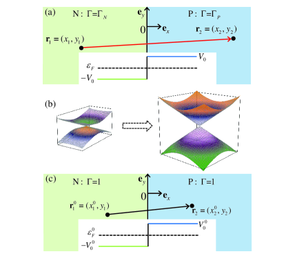
The considered PNJ structure is shown schematically in Fig. 1(a) and it consists of a left N region and a right P region. Each region of the PNJ hosts the anisotropic MDF for which the anisotropy can be different in the N and P regions. In general, the Hamiltonian of the PNJ in Fig. 1(a) has the form:

$$\hat{H}=(\hat{H}_{N}+V_{N})\Theta(-x)+(\hat{H}_{P}+V_{P})\Theta(x),$$ (1)

where $\hat{H}_{i}$ is the intrinsic Hamiltonian of the $i$ ($=$P, N) region, $V_{N}=-V_{0}$ ($V_{P}=V_{0}$) is the gate-induced scalar potential in the N (P) region by assuming $V_{0}>0$ without loss of generality, and $\Theta(x)$ is the step function: $\Theta(x)=1$ for $x>0$ and $\Theta(x)=0$ for $x<0$. In general, the anisotropic MDF of each uniform region can be described by using the Hamiltonian Naumis et al. (2017) $\hat{H}_{i}=v_{F}(\hat{\sigma}_{x}\hat{p}_{x}+\Gamma_{i}\hat{\sigma}_{y}\hat{p}_{y})$. Here, $v_{F}$ represents the Fermi velocity, and $\hat{\sigma}_{x,y}$ and $\hat{p}_{x,y}$ are, respectively, the Pauli operator and the momentum operator. In particular, $\Gamma=\Gamma_{i}$ is introduced to account for the anisotropy of the MDF in the $i$ region, and the specific value of anisotropy depends on the choice of material and the way to tune the energy dispersion, e.g., for the MDF in graphene, the anisotropy can be tuned continuously by reversible strain up to a factor of 5 Pereira et al. (2009) and may be even larger by using a superlattice potential Park et al. (2008a). For the intrinsic Hamiltonian, the energy dispersion is $\varepsilon_{\mu}(\mathbf{k}_{i})=\mu v_{F}\sqrt{k_{i,x}^{2}+\Gamma_{i}^{2}k_{y}^{2}}$ where the index $\mu=+$ ($\mu=-$) is for the conductance (valence) band, $\mathbf{k}_{i}=(k_{i,x},k_{y})$ is the momentum vector, and the corresponding position vector is $\mathbf{r}=(x,y)$. Note that we take units such that $\hbar\equiv 1$ throughout this work.

II.2 Green’s function and the projection method

To investigate the propagation properties of the anisotropic MDF in the PNJ structure, we concentrate on the corresponding propagator or Green’s function (GF), which is defined as $\mathbf{G}(\mathbf{r}_{2},\mathbf{r}_{1},\varepsilon_{F},V_{0})=\langle\mathbf{r}_{2}|(\varepsilon_{F}+i0^{+}-\hat{H})^{-1}|\mathbf{r}_{1}\rangle$ shown by the red line with an arrow in Fig. 1(a). Note that $\mathbf{G}$ is a matrix due to the spinor nature of $\hat{H}$. We have developed a simple and elegant method to derive the GF of isotropic MDF in graphene PNJ structure through the matching technique combining translational invariance along the interface direction of the junction Zhang et al. (2017a). The generalization of this method to the anisotropic MDF is straightforward. However, here we present an alternative but more simple method, i.e, the projection method, which can give the PNJ GF of the anisotropic MDF from that of the isotropic MDF one. To this aim, we project the anisotropic Hamiltonian $\hat{H}_{i}$ into the form $\hat{H}_{i}^{0}=v_{F}(\hat{\sigma}_{x}\hat{p}_{i,x}^{0}+\hat{\sigma}_{y}\hat{p}_{y})$, where $\hat{H}_{i}^{0}\equiv\hat{H}_{i}/\Gamma_{i}$ is the Hamiltonian for the isotropic MDF, and $\hat{p}_{i,x}^{0}\equiv\hat{p}_{x}/\Gamma_{i}$. The corresponding energy dispersion is $\varepsilon_{\mu}^{0}(\mathbf{k}_{i}^{0})=\mu v_{F}\sqrt{(k_{i,x}^{0})^{2}+k_{y}^{2}}$ where $\varepsilon_{\mu}^{0}(\mathbf{k}_{i}^{0})=\varepsilon_{\mu}(\mathbf{k}_{i})/\Gamma_{i}$ presents the projection relation for energy dispersion, $\mathbf{k}_{i}^{0}\mathbf{=(}k_{i,x}^{0},k_{y}\mathbf{)}$ is the projected momentum vector with $k_{i,x}^{0}=k_{i,x}/\Gamma_{i}$, and the corresponding position vector is $\mathbf{r}^{0}\mathbf{=(}x^{0},y\mathbf{)}$ with $x^{0}=\Gamma_{i}x$. Here, to obtain the projection relation $x^{0}=\Gamma_{i}x$, we have used the constraint $[\hat{x},\hat{p}_{x}]=[\hat{x}^{0},\hat{p}_{x}^{0}]=i$ required by performing the Hamiltonian projection. Interestingly, the projection relation for the energy dispersion changes the MDF from an anisotropic to an isotropic one as shown by Fig. 1(b). As a result, we obtain the equivalent PNJ of Fig. 1(a) but based on the isotropic MDF as shown by Fig. 1(c) through the projection relation for the position vector in real space, and the projection relation for the energy dispersion in energy space leads to

$$\varepsilon_{i}^{0}=\frac{\varepsilon_{i}}{\Gamma_{i}}.$$ (2)

Here, $\varepsilon_{N}^{0}=V_{N}^{0}+\varepsilon_{F}^{0}$ and $\varepsilon_{P}^{0}=V_{P}^{0}-\varepsilon_{F}^{0}$ ($\varepsilon_{N}=V_{N}+\varepsilon_{F}$ and $\varepsilon_{P}=V_{P}-\varepsilon_{F}$) represent the doping levels since the Fermi level $\varepsilon_{F}^{0}$ ($\varepsilon_{F}$) lies between the junction potentials of the N and P regions $\varepsilon_{F}^{0}\in[-V_{0}^{0},V_{0}^{0}]$ ($\varepsilon_{F}\in[-V_{0},V_{0}]$)  in the PNJ based on the isotropic (anisotropic) MDF. Obviously, the doping level defines the momentum through the energy dispersions, e.g., $\varepsilon_{i}^{0}(\mathbf{k}_{i}^{0})=v_{F}\sqrt{(k_{i,x}^{0})^{2}+k_{y}^{2}}$. In the two equivalent PNJ structures, the GFs of the isotropic and anisotropic MDFs are related to each other:

$$\mathbf{G}(\mathbf{r}_{2},\mathbf{r}_{1},\varepsilon_{F},V_{0})=\mathbf{G}^{0}(\mathbf{r}_{2}^{0},\mathbf{r}_{1}^{0},\varepsilon_{F}^{0},V_{0}^{0}).$$ (3)

Here, the PNJ GF of the isotropic MDF [see the black line with an arrow in Fig. 1 (c)] is defined as $\hat{G}^{0}(\mathbf{r}_{2}^{0},\mathbf{r}_{1}^{0},\varepsilon_{F}^{0},V_{0}^{0})\equiv\langle\mathbf{r}_{2}^{0}|(\varepsilon_{F}^{0}+i0^{+}-\hat{H}^{0})^{-1}|\mathbf{r}_{1}^{0}\rangle$ where $\hat{H}^{0}$ is the PNJ Hamiltonian of the isotropic MDF in the form:

$$\hat{H}^{0}=(\hat{H}_{N}^{0}+V_{N}^{0}\mathbf{I})\Theta(-x^{0})+(\hat{H}_{P}^{0}+V_{P}^{0}\mathbf{I})\Theta(x^{0}).$$ (4)

Figure 2: Veselago focusing of anisotropic massless Dirac fermions shown by the magnitude of $|G_{21}|$ as a function of $\mathbf{r}_{2}=(x_{2},y_{2})$. Here, $G_{21}$ is the matrix element of the propagator matrix $\mathbf{G}(\mathbf{r}_{2},\mathbf{r}_{1},\varepsilon_{F},V_{0})$. Without loss of generality, we assume $\mathbf{r}_{1}=(-500,0)$, $V_{0}=0.2$, and $\Gamma_{N}=1$. (a) $\varepsilon_{F}=-V_{0}/3$, and $\Gamma_{P}=2$. (b) $\varepsilon_{F}=0$, and $\Gamma_{P}=1$. (c) $\varepsilon_{F}=V_{0}/3$, and $\Gamma_{P}=1/2$. (d) $|G_{21}|$ as a function of $x_{2}$ for $y_{2}=0$ using the same color code as in (a)-(c). In the plot, we define the unit length $a_{0}$ and unit energy $t_{0}$ through $v_{F}=3/2a_{0}t_{0}$ by analogy to graphene Castro Neto et al. (2009).

II.3 Analytical Green’s function of the isotropic MDF

First, we need to derive PNJ GF of the isotropic MDF. By examining the propagation phase and its higher order derivative, we present a detailed analytical derivation of the PNJ GF of the isotropic MDF in Appendix A, which helps to construct the intuitive physical picture for the propagation properties of the isotropic MDF across the PNJ, i.e., the classical trajectories, negative refraction and then Veselago focusing Cheianov et al. (2007). We assume a source at $\mathbf{r}_{1}^{0}=(-a,0)$; the Veselago focusing occurs at its mirror image $\mathbf{r}_{2}^{0}=\mathbf{r}_{1\mathrm{m}}^{0}=(a,0)$ and $\varepsilon_{F}^{0}=0$ in the case of a symmetric junction implying $\varepsilon_{N}^{0}=\varepsilon_{P}^{0}$. The analytical formula for the PNJ GF of the isotropic MDF is $\mathbf{G}^{0}(\mathbf{r}_{1\mathrm{m}}^{0},\mathbf{r}_{1}^{0},\varepsilon_{F}^{0},V_{0}^{0})=\mathcal{G}(V_{0}^{0})$ from the definition

$$\mathcal{G}(V_{0}^{0})\equiv\frac{\rho(V_{0}^{0})}{2i}(\frac{\pi}{2}+2\sigma_{x}).$$ (5)

where $\rho(V_{0}^{0})=V_{0}^{0}/(2\pi v_{F}^{2})$ is the density of states of the isotropic MDF with the doping level $V_{0}^{0}$. Because $\mathcal{G}\propto V_{0}^{0}$ an enhancement of the focusing intensity of the isotropic MDF occurs when increasing the doping level through electrical gating or using other ways. On the other hand, the focusing position has no tunability and must be the mirror image of a fixed source, otherwise the intensity will decrease drastically Zhang et al. (2017a). In fact, there is a hidden parameter dependence, $\mathcal{G}\propto 1/v_{F}^{2}$, which clearly shows the enhancement of the focusing intensity by decreasing the Fermi velocity. If the Fermi velocity can be manipulated, this should be a more effective way than controling the doping level to enhance the focusing intensity since GF has the dependence $\mathcal{G}\propto V_{0}^{0}/v_{F}^{2}$. Due to rapid advances in materials science, many Dirac materials have been discovered with different Fermi velocities providing various opportunities for electron optics, e.g., to enhance the focusing intensity. The general Dirac energy dispersion has two key variables; one is the Fermi velocity and the other is the anisotropy. The manipulation of Fermi velocity is promising for electron optics, which has been investigated previously Barbier et al. (2010), while here we focus on the anisotropy as a new tuning parameter for Veselago focusing.

III Veselago focusing of the anisotropic MDF and its application

III.1 Tunable Veselago focusing by the anisotropic MDF

Using the projection relations between the isotropic and anisotropic MDFs, the propagation properties of the anisotropic MDF across PNJ can be obtained (see Appendix A). Here, we concentrate on Veselago focusing of the anisotropic MDF and highlight its tunable features. The necessary conditions for the Veselago focusing of the anisotropic MDF in PNJ can be given by using the following projection relations:

$$\mathbf{r}_{2}=-\frac{1}{\gamma}\mathbf{r}_{1},\varepsilon_{F}=\frac{1-\gamma}{1+\gamma}V_{0}.$$ (6)

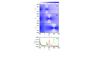
Here, $\mathbf{r}_{1}=\mathbf{r}_{1}^{0}/\Gamma_{N}=(-a/\Gamma_{N},0)$, the equation for $\varepsilon_{F}$ is from Eq. (2) and $\varepsilon_{N}^{0}=\varepsilon_{P}^{0}$ for the symmetric PNJ based on isotropic MDF, and $\gamma=\Gamma_{P}/\Gamma_{N}$ is the ratio of anisotropy of P and N regions. In light of the anisotropy, we can consider three cases; (1) If $\gamma=1$ and $\Gamma_{N}=\Gamma_{P}=1$, it recovers the case for the isotropic MDF, i.e., the Veselago focusing occurs with mirror symmetry. (2) If $\gamma=1$ and $\Gamma_{N}=\Gamma_{P}\neq 1$, it is for anisotropic MDF. Comparing to case (1), the inter-site distance for Veselago focusing can be tuned by the degree of anisotropy, although mirror symmetry is still required. (3) If $\gamma\neq 1$, we also have the anisotropic MDF. In this case, we can tune the focusing position for a fixing source, and Veselago focusing occurs in the asymmetric PNJ in contrast to the previous two cases. For Veselago focusing of the anisotropic MDF, we perform a numerical calculation to show the tunable focusing position by using $\gamma=2$ and $\gamma=1/2$ in Figs. 2(a) and (c), while Fig. 2(b) for the isotropic MDF (namely$\ \gamma=1\$and $\Gamma_{N}=\Gamma_{P}=1)$ is used as a reference.

Furthermore, the intensity of Veselago focusing can also be tuned by changing the anisotropy of the MDF. By using the projection relation, the PNJ GF based on the anisotropic MDF can be expressed as $\mathbf{G}(-\mathbf{r}_{1}/\gamma,\mathbf{r}_{1},\varepsilon_{F},V_{0})=2/(\Gamma_{N}+\Gamma_{P})\mathcal{G}(V_{0})$, where $\mathcal{G}$ given by Eq. (5) is the GF of the isotropic MDF with the doping level $V_{0}$, and the prefactor is introduced by anisotropy of the MDF. Therefore, identical to the isotropic MDF, the focusing intensity of the anisotropic MDF can also be enhanced by increasing $V_{0}$ and by decreasing the Fermi velocity $v_{F}$. Because of the ratio

$$\mathbf{G/}\mathcal{G}=2/(\Gamma_{N}+\Gamma_{P}),$$ (7)

we have the intensity modulation through the anisotropy $\Gamma_{N}$ and $\Gamma_{P}$ of the MDF in the N and P regions. The modulation of the focusing intensity can be clearly seen in Fig. 1(d), which compares the Veselago focusing by considering different values of $\gamma$, and the quantitative relations among the different intensities are fully described by Eq. (7).

Figure 3: The proposed device to probe the masked atom-scale defect in the Cartesian coordinate system ($\mathbf{{e}}_{x}$, $\mathbf{{e}}_{y}$). Graphene is sandwiched between the top and bottom substrates, which may contact the gates Lee et al. (2015); Chen et al. (2016). By using the gates, one can form the PNJ, which has the left N or encapsulated region with green and the right P or the unencapsulated region with blue. By applying a superlattice potential or strain on the substrate below the unencapsulated region, the anisotropic MDF is obtained in the P region with a tunable degree of anisotropy $\Gamma_{P}$. Assuming a defect denoted by the black dot at $\mathbf{r}_{1}=(x_{1},y_{1})$ in the N region, combining the Veselago focusing and the anisotropic MDF of the P region, the focusing image will occur at $\mathbf{r}_{2}=(x_{2},y_{2})=(-x_{1}/\Gamma_{P},y_{1})$ (see Eq. (6) with $\Gamma_{P}>1$) as the red circle or at $\mathbf{r}_{2}^{0}=(x_{2}^{0},y_{2})=(x_{1},y_{1})$ (see Eq. (6) with $\Gamma_{P}=1$) as the black circle, i.e., the realization of the probe of the masked defect. Here, an isotropic MDF is assumed in the N region, i.e., $\Gamma_{N}=1$.

III.2 Potential applications and discussions

In the ballistic regime, even a single scatterer may influence the whole device. A detailed understanding of the influence of such defects on electronic transport is necessary in order to exploit or avoid their influence Settnes et al. (2014). However, it is very difficult to identify masked defects. As a novel application, we propose a device by utilizing the tunable focusing position of the anisotropic MDF to probe masked atom-scale defects in two-dimensional materials with graphene as an example.

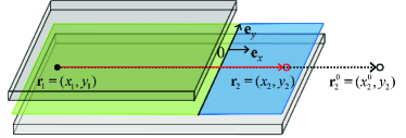
To achieve high mobility, it is necessary to encapsulate graphene with insulating and atomically flat boron nitride crystals. The mismatch between graphene and the boron nitride crystals usually brings a small amount of defects into the graphene samples Dean et al. (2010). Fig. 3 schematically shows the proposed device in which an incomplete encapsulation is proposed, i.e., graphene is sandwiched between two substrates and the area of the bottom substrate is larger than that of the top one. Then, the encapsulated region and the unencapsulated region can be doped into N type and P type through the gates contacting the top and bottom substrates, i.e., a PNJ is formed. Large-area ballistic graphene is not easy to fabricateLee et al. (2015); Chen et al. (2016), so in order to fully utilize the ballistic nature, the encapsulated graphene should be as large as possible, which leads to a small unencapsulated region for the probe. To apply the superlattice potential Park et al. (2008a, b, 2009); Brey and Fertig (2009); Barbier et al. (2008, 2009); Rusponi et al. (2010) or the strain on the substrate Pereira and Castro Neto (2009); Naumis et al. (2017) below the unencapsulated region, one induces the anisotropic MDF in the P region whose degree of anisotropy $\Gamma_{P}$ can be fine-tuned, e.g., make $\Gamma_{P}>1$. If there is a defect denoted by the black dot at $\mathbf{r}_{1}=(x_{1},y_{1})$ in the N region, due to Veselago focusing, one can probe a focusing image denoted by the red circle at $\mathbf{r}_{2}=(x_{2},y_{2})=(-x_{1}/\Gamma_{P},y_{1})$ (see Eq. (6)) with the strong local density of states in the small unencapsulated region by using a scanning tunneling microscope, i.e., the realization of the probe of the masked defect. Here, for the sake of simplicity, the isotropic MDF is assumed in the N region, i.e., $\Gamma_{N}=1$. In the simple case of the PNJ for the isotropic MDF, the Veselago focusing can also be used as a probe for masked defects, but the focusing should be at the mirror image and may be beyond the unencapsulated region, e.g., see the mirror image at $\mathbf{r}_{2}^{0}=(x_{2}^{0},y_{2})=(-x_{1},y_{1})$. Therefore, the tunable focusing position of anisotropic MDF is beneficial to probe masked defects.

Subsequently, we discuss the experimental feasibility of Veselago focusing of the anisotropic MDF. On the one hand, in order to analytically reveal the underlying physics that is generally applicable to various Dirac materials hosting anisotropic MDFs, we consider the PNJ with an abrupt change of anisotropy and on-site potential in our model study. The Veselago focusing is determined by the propagation phase of the MDF between the source and the probe (see Eq. (A2)). Since the MDF propagates mainly in the uniform regions of PNJ, the Veselago focusing should also exist in the presence of a smooth region for the anisotropy and on-site potential. The same physics can also explain the experimental verification of Veselago focusing in the PNJ with a smooth potential region Lee et al. (2015); Chen et al. (2016). To the specific material, e.g., strained graphene whose anisotropy is highly tunable by an elastic or piezoelectric substrate Rold n et al. (2015), the quantitative atomic simulation can be performed by a proper numerical method Zhang et al. (2017b) and is necessary for comparison with future experiments. On the other hand, the realization of Veselago focusing requires high mobility samples. Fortunately, the continuing advances of experimental technology allow the fabrication of high mobility Dirac materials hosting anisotropic MDFs, e.g., graphene with a superlattice potential Forsythe et al. (2017), ZrTe₅ Yuan et al. (2016); Qiu et al. (2016) and Cd₃As₂ Neupane et al. (2014) which are inherently anisotropic. Furthermore, in order to observe Veselago focusing of anisotropic MDF in PNJs based on different Dirac materials, the tunable doping is essential and should not severely reduce sample mobility. Therefore, the electrical gating, which is widely used for two-dimensional systems Lee et al. (2015); Chen et al. (2016), is a better way to dope the sample since the chemical doping may greatly decrease the quality of the sample. In addition, we note that the Veselago focusing of anisotropic MDF could be verified in artificial graphene of cold atoms in light of the recent demonstration of Veselago focusing of isotropic MDFs Leder et al. (2014) and the tunable dispersion properties of cold atoms in an optical lattice Tarruell et al. (2012).

We have shown clearly the Veselago focusing of the anisotropic MDF and its tunability, which will offer easy access to future theoretical and experimental studies. Such Veselago focusing has many potential applications Cheianov et al. (2007); Garcia-Pomar et al. (2008); Moghaddam and Zareyan (2010); Silveirinha and Engheta (2013); Zhao et al. (2013); Bøggild et al. (2017); Zhang et al. (2017a); Hills et al. (2017). Since Veselago focusing in the PNJ based on the anisotropic MDF shows superior tunable features, this must also favor applications. It is convenient to expand our study to incorporate other degrees of freedom such as spin Moghaddam and Zareyan (2010); Zhao et al. (2013); Zhang et al. (2017a) and valley Garcia-Pomar et al. (2008), to consider a three-dimensional MDF Hills et al. (2017), and to examine multiple junctions Garcia-Pomar et al. (2008) and even superlattices Silveirinha and Engheta (2013). Therefore, this study paves the way for an investigation of electron optics behavior of anisotropic MDFs with potential device applications.

IV Conclusions

In this study, we investigated the propagation of anisotropic MDF in a PNJ structure. We constructed projection relations tuning the anisotropic MDF into isotropic MDF. We analytically showed the precise Veselago focusing and stressed its tunable features which are favorable for the design of novel devices to probe (e.g., masked defects) by utilizing the tunable focusing position. This study presents an innovative concept to realize tunable Veselago focusing, and it paves the way for an investigation of electron optics of anisotropic MDF.

Appendix A Analytical derivation of the PNJ GF for isotropic MDF

Here, we present a detailed analytical derivation of the PNJ GF for isotropic MDF, which helps to construct an intuitive physical picture for the propagation properties of isotropic and anisotropic MDF across the PNJ. The PNJ GF of the isotropic MDF is Zhang et al. (2017a),

$$\mathbf{G}^{0}=\int\frac{dk_{y}}{2\pi}e^{i\phi^{0}(k_{y})}t^{0}(\varphi_{N}^{0},\varphi_{P}^{0})\frac{|u_{-}(-k_{P,x}^{0},k_{y})\rangle\langle u_{+}(k_{N,x}^{0},k_{y})|}{iv_{F}k_{N,x}^{0}/k_{N}^{0}}$$ (8)

where $k_{N}^{0}\equiv\varepsilon_{N}^{0}/v_{F}$, $k_{P}^{0}\equiv\varepsilon_{P}^{0}/v_{F}$, $k_{N,x}^{0}\equiv\sqrt{(k_{N}^{0})^{2}-k_{y}^{2}}$, $k_{P,x}^{0}\equiv\sqrt{(k_{P}^{0})^{2}-k_{y}^{2}}$, and the propagation phase is

$$\phi^{0}(k_{y})=k_{y}Y+a\sqrt{(k_{N}^{0})^{2}-k_{y}^{2}}-X\sqrt{(k_{P}^{0})^{2}-k_{y}^{2}}.$$ (9)

Here, for the sake of simplicity, we assume $\mathbf{r}_{1}^{0}=(-a,0)$ and $\mathbf{r}_{2}^{0}=(X,Y)$. In polar coordinates, we use $\varphi_{N}^{0}\in[-\pi/2,\pi/2]$ for the incident angle and $\varphi_{P}^{0}\in[-\pi/2,\pi/2]$ for the refractive angle, as defined by $k_{N,x}^{0}=k_{N}^{0}\cos\varphi_{N}^{0}$ and $k_{P,x}^{0}=k_{P}^{0}\cos\varphi_{P}^{0}$. Then $\varphi_{N}^{0}$ and $\varphi_{P}^{0}$ are connected via $k_{y}=k_{N}^{0}\sin\varphi_{N}^{0}=k_{P}^{0}\sin\varphi_{P}^{0}$ and the transmission coefficient is

$$t^{0}(\varphi_{N}^{0},\varphi_{P}^{0})=\frac{2\cos\varphi_{N}^{0}}{e^{-i\varphi_{N}^{0}}+{e}^{-i\varphi_{P}^{0}}}$$ (10)

corresponding to the propagation of the isotropic MDF from the left N region to the right P region. $t^{0}(\varphi_{N}^{0},\varphi_{P}^{0})$ implies high transparency of PNJ based on the isotropic MDF Katsnelson et al. (2006); Cheianov and Fal’ko (2006), which is an important factor beneficial for the realization of Veselago focusing Cheianov et al. (2007).

The isotropic MDF across the PNJ exhibits novel electron optics behaviors similar to those in metamaterials with a negative refraction index, e.g., Veselago focusing and caustics Cheianov et al. (2007), which can be explained by examining the classical trajectory determined by the propagation phase. The classical trajectory $k_{y,\mathrm{c}}$ going from $\mathbf{r}_{1}^{0}$ to $\mathbf{r}_{2}^{0}$ is determined by $\partial\phi^{0}(k_{y})/\partial k_{y}=0$ as

$$Y=a\tan\theta_{N}^{0}-X\tan\theta_{P}^{0}=R_{N}^{0}\sin\theta_{N}^{0}-R_{P}^{0}\sin\theta_{P}^{0},$$ (11)

where we have introduced the classical incident angle $\theta_{N}^{0}\in[-\pi/2,\pi/2]$ and the refractive angle $\theta_{P}^{0}\in[-\pi/2,\pi/2]$ through

$$\tan\theta_{N}^{0} \equiv\frac{k_{y,\mathrm{c}}}{\sqrt{(k_{N}^{0})^{2}-k_{y,\mathrm{c}}^{2}}},$$ (12)

$$\tan\theta_{P}^{0} \equiv\frac{k_{y,\mathrm{c}}}{\sqrt{(k_{P}^{0})^{2}-k_{y,\mathrm{c}}^{2}}},$$ (13)

and the classical path in the N region and the P region, i.e., $R_{N}^{0}\equiv a/\cos\theta_{N}^{0}$ and $R_{P}^{0}\equiv X/\cos\theta_{P}^{0}$. From $\sin\theta_{N}^{0}=k_{y,\mathrm{c}}/k_{N}^{0}$ and $\sin\theta_{P}^{0}=k_{y,\mathrm{c}}/k_{P}^{0}$, we further have

$$\frac{\sin\theta_{N}^{0}}{\sin\theta_{P}^{0}}=\frac{k_{P}^{0}}{k_{N}^{0}}=\frac{\varepsilon_{P}^{0}}{\varepsilon_{N}^{0}}\equiv n^{0},$$ (14)

which, together with Eq. (11), completely determines $\theta_{N}^{0},\theta_{P}^{0}$ and hence the classical trajectory. Here, the definition of $\theta_{P}^{0}$ makes $n^{0}$ be the magnitude of the effective refractive index of the PNJ, which should be negative Cheianov et al. (2007).

A.1 Veselago focusing and the analytical Green’s function

For the symmetric PNJ, we have $k_{N}^{0}=k_{P}^{0}\equiv k_{F}^{0}$, $\theta_{N}^{0}=\theta_{P}^{0}\equiv\theta^{0}$, and then the classical trajectory is

$$Y=\tan\theta^{0}(a-X)=(R_{N}^{0}-R_{P}^{0})\sin\theta^{0}.$$ (15)

Along the classical path, the phase is

$$\Phi^{0}=k_{F}^{0}\frac{a-X}{\cos\theta^{0}}=\frac{k_{F}^{0}Y}{\sin\theta^{0}}=k_{F}^{0}(R_{N}^{0}-R_{P}^{0})=\mathrm{sgn}(a-X)k_{F}^{0}|\mathbf{r}_{2}^{0}-\mathbf{r}_{1\mathrm{m}}^{0}|,$$ (16)

where $\mathbf{r}_{1\mathrm{m}}^{0}=(a,0)$ is the mirror image of $\mathbf{r}_{1}^{0}=(-a,0)$. In particular, if $\mathbf{r}_{2}^{0}=\mathbf{r}_{1\mathrm{m}}^{0}$, the $0$-order term $\Phi^{0}$ and the arbitrary-order derivative of $\phi^{0}(k_{y})$ vanish for all classical trajectories with different $k_{y,\mathrm{c}}$, which leads to the Veselago focusing.

To derive the analytical GF for the symmetric PNJ, we define the incident angle $\varphi^{0}\in[-\pi/2,\pi/2]$ through $k_{x}^{0}=k_{F}^{0}\cos\varphi^{0}$ and $k_{y}=k_{F}^{0}\sin\varphi^{0}$. Then using the transmission coefficient $t^{0}=\cos\varphi^{0}e^{i\varphi^{0}}$, we have (keeping traveling waves only):

$$\mathbf{G}^{0} \approx\frac{k_{F}^{0}}{2\pi iv_{F}}\int_{-\pi/2}^{\pi/2}\cos\varphi^{0}e^{i\varphi^{0}}d\varphi^{0}\ e^{i\phi^{0}}|u_{-}^{0}(-k_{x}^{0},k_{y})\rangle\langle u_{+}^{0}(k_{x}^{0},k_{y})|$$ (17)

$$=\frac{k_{F}^{0}}{4\pi iv_{F}}(g_{0}+g_{y}\sigma_{x}+g_{z}\sigma_{z}),$$ (18)

where

$$g_{0}^{0} \equiv\int_{-\pi/2}^{\pi/2}\cos^{2}\varphi^{0}e^{i\phi^{0}}d\varphi^{0},$$ (19)

$$g_{y}^{0} \equiv\int_{-\pi/2}^{\pi/2}\cos\varphi^{0}e^{i\phi^{0}}d\varphi^{0},$$ (20)

$$g_{z}^{0} \equiv i\int_{-\pi/2}^{\pi/2}\sin\varphi^{0}\cos\varphi^{0}e^{i\phi^{0}}d\varphi^{0}.$$ (21)

Here, the propagation phase

$$\phi^{0}(\varphi^{0})=k_{F}^{0}[Y\sin\varphi^{0}+(a-X)\cos\varphi^{0}]=\Phi\cos(\varphi^{0}-\theta^{0})$$ (22)

and $\theta^{0}=\tan^{-1}[Y/(a-X)]$ is the classical incident angle and $\Phi^{0}\equiv k_{F}^{0}(a-X)/\cos\theta^{0}$ is the phase along the classical trajectory. For $X=a$ and $Y=0$, i.e., $\mathbf{r}_{2}^{0}=\mathbf{r}_{1\mathrm{m}}^{0}$, we have $\phi^{0}=0$ and hence $g_{0}^{0}=\pi/2$, $g_{y}^{0}=2$, $g_{z}^{0}=0$, i.e.,

$$\mathbf{G}^{0}(\mathbf{r}_{2}^{0},\mathbf{r}_{1}^{0},\varepsilon_{F}^{0},V_{0}^{0})=\frac{k_{F}^{0}}{4\pi iv_{F}}(\frac{\pi}{2}+2\sigma_{x}).$$ (23)

The analytical expression for the GF shows the dependence on the material parameters such as $v_{F}$, $\varepsilon_{F}^{0}$ and $V_{0}^{0}$, but it does not depend on the position vectors $\mathbf{r}_{1}^{0}$ and $\mathbf{r}_{2}^{0}$ as long as $\mathbf{r}_{2}^{0}=\mathbf{r}_{1\mathrm{m}}^{0}$.

A.2 Caustics

For the asymmetric PNJ, there is the caustics corresponding to the singularity of the classical trajectory. For $\mathbf{R}_{2}=(X,Y)\$at certain special locations, the quadratic term of $\phi^{0}(k_{y})$ also vanishes, i.e., $w^{0}\equiv\partial[\phi^{0}(k_{y})]^{2}/\partial k_{y}^{2}=0$ with

$$w^{0}=\frac{a}{q_{N}^{0}\cos^{3}\theta_{N}^{0}}-\frac{X}{q_{P}^{0}\cos^{3}\theta_{P}^{0}}.$$ (24)

Therefore, $w^{0}=0$ leads to the equation

$$\frac{\cos\theta_{N}^{0}}{\cos\theta_{P}^{0}}=(\frac{aq_{P}^{0}}{Xq_{N}^{0}})^{1/3}=(\frac{n^{0}a}{X})^{1/3}.$$ (25)

The caustics curve is determined by Eqs. (11), (14), and (25):

$$Y =\pm\frac{\left[X_{cusp}^{2/3}-X^{2/3}\right]^{3/2}}{\sqrt{1-(n^{0})^{2}}}\ (\mathrm{for}\ n^{0}<1\ \mathrm{and\ }X<X_{cusp}),$$ (26)

$$Y =\pm\frac{\left[X^{2/3}-X_{cusp}^{2/3}\right]^{3/2}}{\sqrt{(n^{0})^{2}-1}}\ (\mathrm{for}\ n^{0}>1\ \mathrm{and\ }X>X_{cusp}).$$ (27)

Note that there is no solution for $n^{0}<1$, $X>X_{cusp}$; and $n^{0}>1,X<X_{cusp}$. Here, $X_{cusp}=n^{0}a$ is the position of the cusp which is a singularity in the density of classical trajectories.

References

- Castro Neto et al. (2009) A. H. Castro Neto, F. Guinea, N. M. R. Peres, K. S. Novoselov, and A. K. Geim, Rev. Mod. Phys. 81, 109 (2009).
- Qi and Zhang (2011) X.-L. Qi and S.-C. Zhang, Rev. Mod. Phys. 83, 1057 (2011).
- Wehling et al. (2014) T. Wehling, A. Black-Schaffer, and A. Balatsky, Advances in Physics 63, 1 (2014).
- Wang et al. (2015) J. Wang, S. Deng, Z. Liu, and Z. Liu, National Science Review 2, 22 (2015).
- Kobayashi et al. (2007) A. Kobayashi, S. Katayama, Y. Suzumura, and H. Fukuyama, Journal of the Physical Society of Japan 76, 034711 (2007).
- Banerjee et al. (2009) S. Banerjee, R. R. P. Singh, V. Pardo, and W. E. Pickett, Phys. Rev. Lett. 103, 016402 (2009).
- Richard et al. (2010) P. Richard, K. Nakayama, T. Sato, M. Neupane, Y.-M. Xu, J. H. Bowen, G. F. Chen, J. L. Luo, N. L. Wang, X. Dai, et al., Phys. Rev. Lett. 104, 137001 (2010).
- Killi et al. (2011) M. Killi, S. Wu, and A. Paramekanti, Phys. Rev. Lett. 107, 086801 (2011).
- Jo et al. (2014) Y. J. Jo, J. Park, G. Lee, M. J. Eom, E. S. Choi, J. H. Shim, W. Kang, and J. S. Kim, Phys. Rev. Lett. 113, 156602 (2014).
- Moon et al. (2011) C.-Y. Moon, J. Han, H. Lee, and H. J. Choi, Phys. Rev. B 84, 195425 (2011).
- Lopez-Bezanilla and Littlewood (2016) A. Lopez-Bezanilla and P. B. Littlewood, Phys. Rev. B 93, 241405 (2016).
- Li et al. (2017) Z. Li, T. Cao, M. Wu, and S. G. Louie, Nano Letters 17, 2280 (2017).
- Park et al. (2011) J. Park, G. Lee, F. Wolff-Fabris, Y. Y. Koh, M. J. Eom, Y. K. Kim, M. A. Farhan, Y. J. Jo, C. Kim, J. H. Shim, et al., Phys. Rev. Lett. 107, 126402 (2011).
- Mullen et al. (2015) K. Mullen, B. Uchoa, and D. T. Glatzhofer, Phys. Rev. Lett. 115, 026403 (2015).
- Yan et al. (2017) M. Yan, H. Huang, K. Zhang, E. Wang, W. Yao, K. Deng, G. Wan, H. Zhang, M. Arita, H. Yang, et al., Nature Communications 8, 257 (2017).
- Pereira and Castro Neto (2009) V. M. Pereira and A. H. Castro Neto, Phys. Rev. Lett. 103, 046801 (2009).
- Naumis et al. (2017) G. G. Naumis, S. Barraza-Lopez, M. Oliva-Leyva, and H. Terrones, Reports on Progress in Physics 80, 096501 (2017).
- Park et al. (2008a) C.-H. Park, L. Yang, Y.-W. Son, M. L. Cohen, and S. G. Louie, Nature Physics 4, 213 (2008a).
- Barbier et al. (2010) M. Barbier, P. Vasilopoulos, and F. M. Peeters, Phys. Rev. B 81, 075438 (2010).
- Park et al. (2008b) C.-H. Park, L. Yang, Y.-W. Son, M. L. Cohen, and S. G. Louie, Phys. Rev. Lett. 101, 126804 (2008b).
- Rusponi et al. (2010) S. Rusponi, M. Papagno, P. Moras, S. Vlaic, M. Etzkorn, P. M. Sheverdyaeva, D. Pacilé, H. Brune, and C. Carbone, Phys. Rev. Lett. 105, 246803 (2010).
- Lu et al. (2016) H.-Y. Lu, A. S. Cuamba, S.-Y. Lin, L. Hao, R. Wang, H. Li, Y. Zhao, and C. S. Ting, Phys. Rev. B 94, 195423 (2016).
- Cheianov et al. (2007) V. V. Cheianov, V. Fal’ko, and B. L. Altshuler, Science 315, 1252 (2007).
- Williams et al. (2011) J. R. Williams, T. Low, M. S. Lundstrom, and C. M. Marcus, Nat Nano 6, 222 (2011).
- Rickhaus et al. (2013) P. Rickhaus, R. Maurand, M.-H. Liu, M. Weiss, K. Richter, and C. Schonenberger, Nat. Commun. 4, 2342 (2013).
- Taychatanapat et al. (2015) T. Taychatanapat, J. Y. Tan, Y. Yeo, K. Watanabe, T. Taniguchi, and B. Özyilmaz, Nature Communications 6, 6093 (2015).
- Pendry (2007) J. B. Pendry, Science 315, 1226 (2007), ISSN 0036-8075.
- Garcia-Pomar et al. (2008) J. L. Garcia-Pomar, A. Cortijo, and M. Nieto-Vesperinas, Phys. Rev. Lett. 100, 236801 (2008).
- Moghaddam and Zareyan (2010) A. G. Moghaddam and M. Zareyan, Phys. Rev. Lett. 105, 146803 (2010).
- Silveirinha and Engheta (2013) M. G. Silveirinha and N. Engheta, Phys. Rev. Lett. 110, 213902 (2013).
- Zhao et al. (2013) L. Zhao, P. Tang, B.-L. Gu, and W. Duan, Phys. Rev. Lett. 111, 116601 (2013).
- Milovanovic et al. (2015) S. P. Milovanovic, D. Moldovan, and F. M. Peeters, J. Appl. Phys. 118, 154308 (2015).
- Bøggild et al. (2017) P. Bøggild, J. M. Caridad, C. Stampfer, G. Calogero, N. R. Papior, and M. Brandbyge, Nature Communications 8, 15783 (2017).
- Zhang et al. (2017a) S.-H. Zhang, J.-J. Zhu, W. Yang, and K. Chang, 2D Materials 4, 035005 (2017a).
- Hills et al. (2017) R. D. Y. Hills, A. Kusmartseva, and F. V. Kusmartsev, Phys. Rev. B 95, 214103 (2017).
- Lee et al. (2015) G.-H. Lee, G.-H. Park, and H.-J. Lee, Nat. Phys. 11, 925 (2015).
- Chen et al. (2016) S. Chen, Z. Han, M. M. Elahi, K. M. M. Habib, L. Wang, B. Wen, Y. Gao, T. Taniguchi, K. Watanabe, J. Hone, et al., Science 353, 1522 (2016).
- Hassler et al. (2010) F. Hassler, A. R. Akhmerov, and C. W. J. Beenakker, Phys. Rev. B 82, 125423 (2010).
- P terfalvi et al. (2012) C. G. P terfalvi, L. Oroszl ny, C. J. Lambert, and J. Cserti, New Journal of Physics 14, 063028 (2012).
- Pereira et al. (2009) V. M. Pereira, A. H. Castro Neto, and N. M. R. Peres, Phys. Rev. B 80, 045401 (2009).
- Settnes et al. (2014) M. Settnes, S. R. Power, D. H. Petersen, and A.-P. Jauho, Phys. Rev. Lett. 112, 096801 (2014).
- Dean et al. (2010) C. R. Dean, A. F. Young, I. Meric, C. Lee, L. Wang, S. Sorgenfrei, K. Watanabe, T. Taniguchi, P. Kim, K. L. Shepard, et al., Nature Nanotechnology 5, 722 (2010).
- Park et al. (2009) C.-H. Park, Y.-W. Son, L. Yang, M. L. Cohen, and S. G. Louie, Phys. Rev. Lett. 103, 046808 (2009).
- Brey and Fertig (2009) L. Brey and H. A. Fertig, Phys. Rev. Lett. 103, 046809 (2009).
- Barbier et al. (2008) M. Barbier, F. M. Peeters, P. Vasilopoulos, and J. M. Pereira, Phys. Rev. B 77, 115446 (2008).
- Barbier et al. (2009) M. Barbier, P. Vasilopoulos, F. M. Peeters, and J. M. Pereira, Phys. Rev. B 79, 155402 (2009).
- Rold n et al. (2015) R. Rold n, A. Castellanos-Gomez, E. Cappelluti, and F. Guinea, Journal of Physics: Condensed Matter 27, 313201 (2015).
- Zhang et al. (2017b) S.-H. Zhang, W. Yang, and K. Chang, Phys. Rev. B 95, 075421 (2017b).
- Forsythe et al. (2017) C. Forsythe, X. Zhou, T. Taniguchi, K. Watanabe, A. Pasupathy, P. Moon, M. Koshino, P. Kim, and C. R. Dean, ArXiv (2017), eprint 1710.01365.
- Yuan et al. (2016) X. Yuan, C. Zhang, Y. Liu, A. Narayan, C. Song, S. Shen, X. Sui, J. Xu, H. Yu, Z. An, et al., Npg Asia Materials 8, e325 (2016).
- Qiu et al. (2016) G. Qiu, Y. Du, A. Charnas, H. Zhou, S. Jin, Z. Luo, D. Y. Zemlyanov, X. Xu, G. J. Cheng, and P. D. Ye, Nano Letters 16, 7364 (2016).
- Neupane et al. (2014) M. Neupane, S.-Y. Xu, R. Sankar, N. Alidoust, G. Bian, C. Liu, I. Belopolski, T.-R. Chang, H.-T. Jeng, H. Lin, et al., Nature Communications 5, 3786 (2014).
- Leder et al. (2014) M. Leder, C. Grossert, and M. Weitz, Nature Communications 5, 3327 (2014).
- Tarruell et al. (2012) L. Tarruell, D. Greif, T. Uehlinger, G. Jotzu, and T. Esslinger, Nature 483, 302 (2012).
- Katsnelson et al. (2006) M. I. Katsnelson, K. S. Novoselov, and A. K. Geim, Nat. Phys. 2, 620 (2006).
- Cheianov and Fal’ko (2006) V. V. Cheianov and V. I. Fal’ko, Phys. Rev. B 74, 041403 (2006).