Topological nodal line semimetals in holography

Abstract

We show a holographic model of a strongly coupled topological nodal line semimetal (NLSM) and find that the NLSM phase could go through a quantum phase transition to a topologically trivial state. The dual fermion spectral function shows that there are multiple Fermi surfaces each of which is a closed nodal loop in the NLSM phase. The topological structure in the bulk is induced by the IR interplay between the dual mass operator and the operator that deforms the topology of the Fermi surface. We propose a practical framework for building various strongly coupled topological semimetals in holography, which indicates that at strong coupling topologically nontrivial semimetal states generally exist.

1 Introduction

During the last decade, our understanding towards topological states of matter has grown enormously in condensed matter physics. Examples of topological states of matter include topological insulators, topological Weyl semimetals (WSMs)/NLSMs, anomalous Hall states, and topological superconductors (see e.g. Witten:2015aoa ; review-tsm for a review). Most properties of the topological systems that we have known were built on the weakly coupled picture. An important challenge in the understanding of topological states of matter is to consider the effect of interactions, especially strong interactions, on the topological structures of these systems. Weakly coupled nontrivial topological structure could be destroyed by strong interactions or new strongly coupled topological states of matter could arise. This has been a rapidly growing research area in condensed matter during the recent years. However, it remains quite difficult to attack this problem due to the lack of band structure and no notion of quasiparticles and technical difficulty at strong coupling in the condensed matter physics, especially for gapless topological systems. Some attempts in this direction could be found in interaction1 ; interaction2 .

To study strongly coupled topological states of matter, a very powerful tool from string theory, the AdS/CFT correspondence, which maps a $d+1$ dimensional strongly coupled field theory to a $d+2$ dimensional weakly coupled classical gravitational theory, would be extremely helpful. As a strong-weak duality, AdS/CFT has obtained lots of success in its applications to strongly coupled condensed matter systems book ; book0 ; review . It is, however, still a relatively undeveloped research area to incorporate topological states of matter into the holographic dictionary. Some previous attempts could be found in e.g. HoyosBadajoz:2010ac ; Kristjansen:2016rsc ; Seo:2017oyh for topological insulator and WeiLi ; Bergman:2010gm for quantum Hall states. Here we shall explore what holography can tell about the strongly interacting topological semimetals.

An important question is if there exists a general framework for holographic topological states of matter and to find the corresponding bulk topological structure. As a first step to answer these questions and inspired by our previous work Landsteiner:2015pdh on a holographic model of strongly coupled WSM state, we will start from building a holographic model of topological NLSM, which is a gapless topological state of matter whose Fermi surface forms closed loops in momentum space. We will show its dual fermion spectral function behavior and reveal the common mathematical structure of topology in the gravitational solutions that the NLSMs and WSMs share. In particular, this bulk topological structure could be generalized to a general paradigm in holography to describe strongly coupled gapless topological states of matter.

In the following of this paper we will first give an example of a new entry in the holographic dictionary of topological states of matter: the holographic topological nodal line semimetal in Sec. 2. Then the behavior of the corresponding fermion spectral functions of the nodal line semimetal will be shown in Sec. 3. In Sec. 4 we point out the general bulk topological structure of topological semimetal states. Appendices A, B, C contain the equations of motion, free energy calculations of the system and the discussion at the probe limit.

2 Holographic topological nodal line semimetals

A NLSM burkov1 has a nontrivial shape of Fermi surface where Fermi nodal points form a circle under certain symmetries, e.g. mirror reflection symmetry (see rev1 for a review). A topologically nontrivial NLSM cannot be gapped by small perturbations unless passing through a topological phase transition to a trivial state.

2.1 A field theoretical model

To get some hint for building the dictionary of this model, we first take a look at a simple weakly coupled field theory model that represents a nodal line semimetal. The Lagrangian is

$$\mathcal{L}=i\bar{\psi}\big{(}\gamma^{\mu}\partial_{\mu}-m-\gamma^{\mu\nu}b_{\mu\nu}\big{)}\psi$$ (1)

where $\gamma^{\mu\nu}=\frac{i}{2}[\gamma^{\mu},\gamma^{\nu}]\,$ and $b_{\mu\nu}=-b_{\nu\mu}$ is an antisymmetric two form field. Note that to be consistent with the gravity calculations, we take the $(-,+,+,+)$ signature. We turn on a nonzero constant $b_{xy}$ component of the two form field and the energy spectrum of the eigenstates of this system are therefore

$$E_{\pm}=\pm\sqrt{k_{z}^{2}+\Big{(}2b_{xy}\pm\sqrt{m^{2}+k_{x}^{2}+k_{y}^{2}}\,\Big{)}^{2}}\,.$$ (2)

For $m^{2}<4b_{xy}^{2}$, the system is a topological nodal line semimetal with Fermi points forming a connected circle with radius $\sqrt{4b_{xy}^{2}-m^{2}}$ in the momentum space. In this parameter regime we can see that the system cannot be gapped by small perturbations like an ordinary Dirac field, i.e. a small perturbation in $m$ cannot gap this system. For $m^{2}>4b_{xy}^{2}$, the system becomes an insulator and $m^{2}=4b_{xy}^{2}$ is the quantum transition point of this topological phase transition. In the nodal line phase, we see that close to the Fermi line, the dispersion behaves as linear in $\sqrt{k_{x}^{2}+k_{y}^{2}}-\sqrt{4b_{xy}^{2}-m^{2}}$ with velocity $\sqrt{1-\frac{m^{2}}{4b_{xy}^{2}}}$ when $k_{z}=0$ and linear in $k_{z}$ with velocity $1$ when $\sqrt{k_{x}^{2}+k_{y}^{2}}=\sqrt{4b_{xy}^{2}-m^{2}}$.

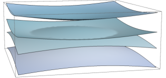
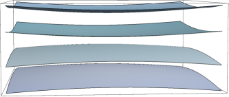
Figure 1: The energy spectrum as a function of $k_{x},k_{y}$ for $k_{z}=0$. Left: there is a nodal line at the band crossing when $m^{2}<4b_{xy}^{2}$. Right: for $m^{2}>4b_{xy}^{2}$ the system is gapped.

We can see that the phase described by (1) for $m^{2}<4b_{xy}^{2}$ should be a topologically nontrivial nodal line semimetal. Other components of $b_{\mu\nu}$ would play a similar role and produce a nodal line semimetal with slight difference in the spectrum, e.g. $b_{tz}$ would produce an accidental nodal line semimetal.

The new two form field $b_{\mu\nu}$ term does not break the conservation of the eletric current $J^{\mu}=\bar{\psi}\gamma^{\mu}\psi$ while does not conserve the axial current $J_{5}^{\mu}=\bar{\psi}\gamma^{\mu}\gamma^{5}\psi$. We have the following conservation equations

$$\partial_{\mu}J^{\mu} = 0\,,$$ (3)

$$\partial_{\mu}J_{5}^{\mu} = -2m\bar{\psi}\gamma^{5}\psi-2b_{\mu\nu}\bar{\psi}\gamma^{\mu\nu}\gamma^{5}\psi\,,$$ (4)

where we have ignored the anomaly terms.

Meanwhile, let us elaborate more on the differences between Weyl Semimetal (WSM) and nodal line semimetal (NLSM) which are two different novel examples of gapless topological states of matter. In the former case two Weyl points are separated at a distance $b$ while the latter Weyl points form a 1D circle. The low energy effective field theory for weakly coupled WSM and NLSM are different, although both of them can be described as a Dirac fermion coupled to an external field. In the former case, a time reversal symmetry breaking parameter axial $A_{z}$ is crucial, while for the latter, a two form effective field $b_{xy}$ is crucial which breaks both time reversal and charge conjugate.

2.2 The holographic model

A weakly coupled NLSM model is shown in the above subsection, where a coupling term $\bar{\psi}\gamma^{\mu\nu}\psi$ is responsible for deforming the Fermi point to a closed loop. It is a new nontrivial topological semimetal phase compared to WSM in which the Fermi point is seperated to two Weyl points. Motivated by the weakly coupled mechanism, we utilize a massive two form field $B_{ab}$ to be dual to an antisymmetric operator which is though not exactly the $\bar{\psi}\gamma^{\mu\nu}\psi$ operator and introduce an axially charged scalar field $\Phi$ to be dual to the operator $\bar{\psi}\psi$ whose source term breaks the axial symmetry and represents the gap effect. We consider

$$S = \int d^{5}x\sqrt{-g}\bigg{[}\frac{1}{2\kappa^{2}}\bigg{(}R+\frac{12}{L^{2}}\bigg{)}-\frac{1}{4}\mathcal{F}^{2}-\frac{1}{4}F^{2}+\frac{\alpha}{3}\epsilon^{abcde}A_{a}\bigg{(}3\mathcal{F}_{bc}\mathcal{F}_{de}+F_{bc}F_{de}\bigg{)}$$ (5)

$$-(D_{a}\Phi)^{*}(D^{a}\Phi)-V_{1}(\Phi)-\frac{1}{3\eta}\big{(}\mathcal{D}_{[a}B_{bc]}\big{)}^{*}\big{(}\mathcal{D}^{[a}B^{bc]}\big{)}-V_{2}(B_{ab})-\lambda|\Phi|^{2}B_{ab}^{*}B^{ab}\bigg{]}$$

where $\mathcal{F}_{ab}=\partial_{a}V_{b}-\partial_{b}V_{a}$ is the vector gauge field strength, $F_{ab}=\partial_{a}A_{b}-\partial_{b}A_{a}$ is the axial gauge field strength, $D_{a}=\nabla_{a}-iq_{1}A_{a}$, $\mathcal{D}_{a}=\nabla_{a}-iq_{2}A_{a}$ and

$$\mathcal{D}_{[a}B_{bc]} = \partial_{a}B_{bc}+\partial_{b}B_{ca}+\partial_{c}B_{ab}$$ (6)

$$~{}-iq_{2}A_{a}B_{bc}-iq_{2}A_{b}B_{ca}-iq_{2}A_{c}B_{ab}\,.$$

$B_{ab}$ is also axially charged as the dual operator explicitly breaks the axial symmetry. The potential terms are

$$V_{1}=m_{1}^{2}|\Phi|^{2}+\frac{\lambda_{1}}{2}|\Phi|^{4}\,,~{}~{}~{}~{}V_{2}=m_{2}^{2}B^{*}_{ab}B^{ab}\,,$$ (7)

where $m_{1}$ and $m_{2}$ are the mass parameters of the scalar and the two form field. $B_{ab}$ has a mass term because it does not correspond to a conserved operator and we will turn on the $B_{xy}$ component in the following. The $\lambda$ term denotes the interaction effect between the operators $\bar{\psi}\psi$ and the antisymmetric operator, which is important to the existence of the topological structure and the topological phase transition. Similar to the holographic WSM Landsteiner:2015pdh , we introduce the $\lambda_{1}$ term because it is not possible to find nonsingular solutions without this term. $\lambda_{1}$ characterises the number of UV degrees of freedom that does not gap in the IR. This indicates that this simple holographic system cannot be completely gapped in the IR and could only be partially gapped at most. The equations of motion, choice of parameters and current conservation equations can be found in appendix A.

From the weakly coupled theory, we see that the operators $\bar{\psi}\psi$ and $\bar{\psi}\gamma^{5}\psi$ correspond to the real and imaginary parts of the complex scalar field in the bulk and the operators $\bar{\psi}\gamma^{\mu\nu}\psi$ and $\bar{\psi}\gamma^{\mu\nu}\gamma^{5}\psi$ should have similar properties. However, the operators $\bar{\psi}\gamma^{\mu\nu}\psi$ and $\bar{\psi}\gamma^{\mu\nu}\gamma^{5}\psi$ not independent indicating that the dual field $B_{ab}$ should have a self-dual property. To avoid this problem, here we instead consider an operator different from $\bar{\psi}\gamma^{\mu\nu}\psi$ which nevertheless is antisymmetric in the two indices and has no self duality properties. Note that a previous holographic model considered the self-duality effect Alvares:2011wb .

Three types of solutions at zero temperature.– To study the quantum phase transition of the system, we shall focus on solutions at zero temperature. We choose the ansatz of the background to be

$$ds^{2} = u(-dt^{2}+dz^{2})+\frac{dr^{2}}{u}+f(dx^{2}+dy^{2})\,,$$

$$\Phi = \phi(r)\,,$$ (8)

$$B_{xy} = B(r)\,.$$

At the UV boundary, the fields $\phi(r)$ and $B(r)$ behave as

$$\phi=\frac{M}{r}+\cdots\,,~{}~{}~{}~{}~{}B=br+\cdots\,,$$ (9)

where $M$ and $b$ correspond to the source for the two dual operators. All through the paper we will work at $b=1$, i.e. all dimensionful parameters are compared to $b$. To solve these equations, we need to identify the near horizon boundary condition. It turns out we have three different kinds of near horizon geometries. With proper irrelevant deformations, these solutions flow to the UV AdS₅ with different boundary values of $M/b$.

Topological phase. The near horizon solution for the topological phase is

$$u = \frac{1}{8}(11+3\sqrt{13})r^{2}\Big{(}1+\delta u\,r^{\alpha_{1}}\Big{)}\,,$$

$$f = \sqrt{\frac{2\sqrt{13}}{3}-2}\,b_{0}r^{\alpha}\Big{(}1+\delta f\,r^{\alpha_{1}}\Big{)}\,,$$

$$\phi = \phi_{0}r^{\beta}\,,$$

$$B = b_{0}r^{\alpha}\Big{(}1+\delta b\,r^{\alpha_{1}}\Big{)}\,,$$

where $(\alpha,\beta,\alpha_{1})=(0.183,0.290,1.273)$, $(\delta f,\delta b)=(-2.616,-0.302)\delta u$ for the parameter values that we have fixed above. $b_{0}$ can be set to $1$ by the transformation $(x,y)\to c(x,y)$. Moreover, the near horizon geometry has a Lifshitz symmetry at leading order

$$(t,z,r^{-1})\to c(t,z,r^{-1})\,,~{}~{}~{}(x,y)\to c^{\alpha/2}(x,y)\,,$$ (10)

which can be used to set $\delta u=\pm 1$ and $\delta u=-1$ flows the geometry to AdS₅. Thus in the IR, we only have a unique free parameter $\phi_{0}$.

We integrate this solution to the boundary and for this type of near horizon boundary conditions we can only find solutions for $M/b<1.717$. When the value of $\phi_{0}$ is zero, the boundary reaches $M/b=0$. When $\phi_{0}$ grows, $M/b$ becomes larger and closer to the critical value $1.717$. To see that this corresponds to the NLSM phase, we will give evidence from fermion spectral functions below.

Critical point. The near horizon solution for the critical point including irrelevant deformations is

$$u = u_{c}r^{2}(1+\delta u\,r^{\beta_{1}})\,,$$

$$f = f_{c}r^{\alpha_{c}}(1+\delta f\,r^{\beta_{1}})\,,$$

$$\phi = \phi_{c}(1+\delta\phi\,r^{\beta_{1}})\,,$$

$$B = b_{c}r^{\alpha_{c}}(1+\delta b\,r^{\beta_{1}})\,,$$

with

$$(u_{c},f_{c},\alpha_{c},\phi_{c})\simeq(3.076,0.828b_{c},0.292,0.894)\,,$$

and

$$\beta_{1}=1.272\,,~{}~{}~{}~{}~{}(\delta u,\delta f,\delta b)=(1.177,-2.771,-0.409)\delta\phi\,.$$

Using the transformation $(x,y)\to c(x,y)$, we set $b_{c}=1$. Without the deformation, the near horizon has the same type of Lifshitz symmetry (10) with $\alpha$ replaced by $\alpha_{c}$. Utilizing this symmetry, $\delta\phi$ could be chosen to be $\delta\phi=-1$ to flow the geometry to $AdS_{5}$ at the boundary. There is no free parameter in the IR and the geometry is unique. At the boundary we find the critical $M/b\simeq 1.717$.

Trivial phase. The near horizon solution for the trivial phase is

$$u = \big{(}1+\frac{3}{8\lambda_{1}}\big{)}r^{2}\,,$$

$$f = r^{2}\,,$$

$$\phi = \sqrt{\frac{3}{\lambda_{1}}}+\phi_{1}r^{\frac{2\sqrt{160\lambda_{1}^{2}+84\lambda_{1}+9}}{3+8\lambda_{1}}-2}\,,$$

$$B = b_{1}r^{2\sqrt{2}\sqrt{\frac{3\lambda+\lambda_{1}}{3+8\lambda_{1}}}}\,.$$

Note that the $\phi_{1}$- and $b_{1}$-terms are irrelevant deformations that flow the near AdS₅ leading order exact solution to asymptotic $AdS_{5}$ solutions. For this type of near horizon boundary conditions we can only find solutions for $M/b>1.717$. For the critical and the trivial solutions here, the scalar field $\phi$ is a finite constant at the horizon and the system is partially gapped.

In Fig. 2, we show the bulk behavior of $\phi$ and $B/f$ for different values of $M/b$ which correspond to different near horizon geometries. Close to the critical $M/b$, the near horizon solution flows to the critical solution quickly. Fig. 3 is the free energy of this system, which shows that the system is continuous when crossing the quantum phase transition point. From Figs. 2 and 3 we could see that though the phase transition is a very continuous one, the bulk IR solutions seem to be discontinuous. This is a common feature of many holographic continuous phase transitions, especially BKT phase transitions Iqbal:2011aj ; Donos:2012js ; Hartnoll:2011pp ; Liu:2013yaa . Near the transition critical point of such systems, there exists an IR critical scale below which the solutions of the two phases (or the solution of one of the phases when there is only one solution at each region of the phase diagram) start to deviate from the critical solution while above this IR critical scale, the solutions of the two phases (or the solution of one of the phases) converge to the critical solution. This IR scale depends on how far the system is way from the critical point and could be exponentially small near the critical point for very continuous phase transitions, e.g. BKT phase transitions Iqbal:2011aj . As the system approaches the transition critical point, this IR scale decreases and becomes infinitely small so that the solutions of the two phases converge to the critical solution for almost all the bulk spacetime. Thus the free energy also shows a very continuous behavior even though the IR solutions look discontinuous.

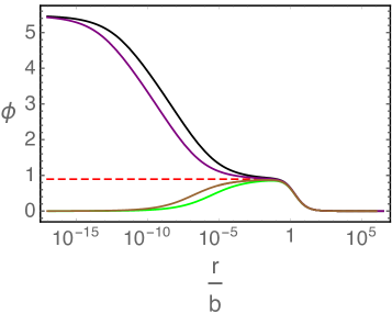
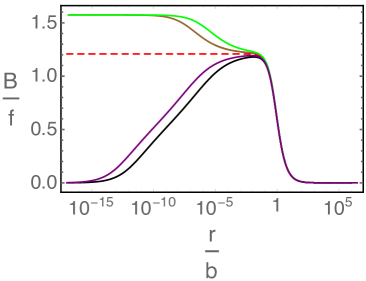
Figure 2: The bulk profile for the scalar field $\phi$ and the two form field $B/f$ for different values of $M/b=1.682$ (green), $1.702$ (brown), $1.717$ (red), $1.733$ (purple), $1.750$ (black).

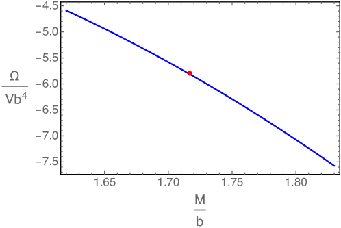
Figure 3: The dependance of free energy on $M/b$. The red dot is the value of free energy density at the critical point. Approaching the transition point from both the topological phase and the trivial phase, the system is continuous and smooth.

Note that the mechanism for the topological quantum phase transition here is different from the Breitenlohner-Freedman bound mechanism for many holographic quantum phase transitions, including holographic superconductors Iqbal:2011aj , metal-insulator phase transitions Donos:2012js , etc.. Here the IR scaling dimensions of the fields do not change for each phase and different phases are due to different values of sources at the UV. There is no local order operator associated with this phase transition similar to the holographic quantum phase transitions in Hartnoll:2011pp .

3 Fermion spectral functions

For NLSMs there is no smoking gun transport coefficient like anomalous Hall conductivity for WSMs. An immediate and straightforward test would be to see if there is indeed a closed nodal loop from the dual fermion spectral functions. We will show that the fermion spectral function in this system confirms that in the nodal line semimetal phase, there is indeed a peak at $k_{x}^{2}+k_{y}^{2}=k_{0}^{2}$ where the value of $k_{0}$ decreases with $M/b$ increasing and finally becomes zero at the critical point. We expect that we could also see the nontrivial topology in the structure of the fermion spectral functions, which we hope to report in the future work.

The prescription for calculating the holographic fermion spectral function could be found in Iqbal:2009fd ; Liu:2009dm ; Cubrovic:2009ye . In five dimensions, one bulk Dirac spinor corresponds to one chirality of boundary Weyl spinor. We utilize two spinors with one spinor to use standard quantization to calculate the dual fermion spectral function and change the sign of Fermi mass $m$ and use alternative quantization to calculated the fermion spectral function of the other chirality.since in both the holographic Weyl/nodal line semimetal model, the two chiralities interact with each other due to the axial symmetry breaking terms. As can be seen from formula (4) both the mass term and the $b_{\mu\nu}$ term break the axial symmetry and couple spinors of two chiralities together. The action of the two spinors $\Psi_{1}$ and $\Psi_{2}$ are

$$S_{\text{fermion}}=S_{1}+S_{2}+S_{\text{int}}\,,$$ (11)

where

$$S_{1} = \int d^{5}x\sqrt{-g}i\bar{\Psi}_{1}\big{(}\Gamma^{a}D_{a}-m_{f}\big{)}\Psi_{1}\,,$$

$$S_{2} = \int d^{5}x\sqrt{-g}i\bar{\Psi}_{2}\big{(}\Gamma^{a}D_{a}+m_{f}\big{)}\Psi_{2}\,,$$

$$S_{\text{int}} = -\int d^{5}x\sqrt{-g}\big{(}i\eta_{1}\Phi\bar{\Psi}_{1}\Psi_{2}+i\eta_{1}^{*}\Phi^{*}\bar{\Psi}_{2}\Psi_{1}\big{)}+S_{B}\,,$$

and

$$S_{B}=\int d^{5}x\sqrt{-g}i(\eta_{2}B_{ab}\bar{\Psi}_{1}\Gamma^{ab}\gamma^{5}\Psi_{2}-\eta_{2}^{*}B_{ab}^{*}\bar{\Psi}_{2}\Gamma^{ab}\gamma^{5}\Psi_{1})\,.$$ (12)

Note that the Lorentz invariance in the tangent space has been explicitly broken in the bulk and this is the exact choice to produce the specific coupling for the fermions to generate a nodal line in the spectrum. Here

$$D_{a}=\partial_{a}-\frac{i}{4}\omega_{\underline{m}\underline{n},a}\Gamma^{\underline{m}\underline{n}}-iq_{3}A_{a}$$ (13)

where $\omega_{\underline{m}\underline{n},a}$ is the bulk spin connection. Note that $a$ and $\underline{m}$ are the bulk spacetime index and the tangent space index respectively. $\bar{\Psi}=\Psi^{\dagger}\Gamma^{\underline{t}}$, $\Gamma^{ab}=e_{\underline{m}a}e_{\underline{n}b}\frac{i}{2}[\Gamma^{\underline{m}},\Gamma^{\underline{n}}]$. $m_{f}$ is the mass of the bulk spinor which determines the scaling dimension of the dual Fermionic operator and we choose $m_{f}=-1/4$ so that there could be poles in the dual fermion spectral functions Iqbal:2009fd . We also set $\eta_{1}=\eta_{2}=1$. The equations of motion are

$$\big{(}\Gamma^{a}D_{a}-m_{f}\big{)}\Psi_{1}-\big{(}\eta_{1}\phi-\eta_{2}B_{ab}\Gamma^{ab}\gamma^{5}\big{)}\Psi_{2}=0\,,$$

$$\big{(}\Gamma^{a}D_{a}+m_{f}\big{)}\Psi_{2}-\big{(}\eta_{1}\phi+\eta_{2}^{*}B_{ab}^{*}\Gamma^{ab}\gamma^{5}\big{)}\Psi_{1}=0\,,$$ (14)

where the five dimensional $\Gamma$ functions are $\Gamma^{\underline{\mu}}=\gamma^{\mu}$, $\Gamma^{\underline{r}}=\gamma^{5}.$ We expand the fermion field as

$$\Psi_{l}=(uf)^{-1/2}\psi_{l}e^{-i\omega t+ik_{x}x+ik_{y}y+ik_{z}z}$$

with $l=(1,2)$ and the corresponding Dirac equation can be written as

$$\Bigg{(}\Gamma^{\underline{r}}\partial_{r}+\frac{1}{u}\Big{(}-i\omega\Gamma^{\underline{t}}+ik_{z}\Gamma^{\underline{z}}\Big{)}+\frac{1}{\sqrt{uf}}\Big{(}ik_{x}\Gamma^{\underline{x}}+ik_{y}\Gamma^{\underline{y}}\Big{)}+(-1)^{l}\frac{m_{f}}{\sqrt{u}}\Bigg{)}\psi_{l}$$

$$~{}~{}~{}~{}~{}-\Bigg{(}\eta_{1}\frac{\phi}{\sqrt{u}}+(-1)^{l}\eta_{2}\frac{b}{\sqrt{u}f}\Gamma^{\underline{x}\underline{y}}\gamma^{5}\Bigg{)}\psi_{3-l}=0\,.$$ (15)

We can solve this as a coupled system of 8 functions. At the horizon the ingoing boundary condition depends on the near horizon geometry of each phase. For the topologically trivial phase, the near horizon ingoing solution for nonzero $k$ while $\omega\to 0$ is real just as the pure AdS₅ case in Iqbal:2009fd . Thus the imaginary part of the Green’s function is automatically zero for nonzero $k$ and the Fermi momentum should stay at $k=0$. For the topologically nontrivial and critical phases, the near horizon ingoing boundary condition is

$$\psi_{l}\simeq e^{\frac{i\sqrt{w^{2}-k_{z}^{2}}}{u_{0}r}}\begin{pmatrix}z^{l}_{1}(1+\cdots)\\ \vspace{-.3cm}\\ z^{l}_{2}(1+\cdots)\\ \vspace{-.3cm}\\ i\frac{\sqrt{\omega^{2}-k_{z}^{2}}}{\omega-k_{z}}z^{l}_{1}(1+\cdots)\\ \vspace{-.3cm}\\ i\frac{\sqrt{\omega^{2}-k_{z}^{2}}}{\omega+k_{z}}z^{l}_{2}(1+\cdots)\end{pmatrix}$$ (16)

with $l=(1,2)$ for $w>k_{z}$, where $``\cdots"$ denote subleading terms. This is because the terms proportional to $k_{x}$ and $k_{y}$ are not so important compared to terms with $\omega$ and $k_{z}$ as $g^{xx}$ is not as divergent as $g^{zz}$ and $g^{tt}$ at the horizon. This also means that for nonzero $k_{z}$ and $\omega\to 0$, the retarded Green’s function is real and the Fermi surface could only stay at $k_{z}=0$, which is consistent with the fact that this corresponds to a nodal line semimetal in the $x$-$y$ plane.

Near the boundary $r\to\infty$,

$$\psi_{l}=\begin{pmatrix}a^{l}_{1}&&r^{m_{f}}+\cdots\\ \vspace{-.3cm}\\ a^{l}_{2}&&r^{m_{f}}+\cdots\\ \vspace{-.3cm}\\ a^{l}_{3}&&r^{-m_{f}}+\cdots\\ \vspace{-.3cm}\\ a^{l}_{4}&&r^{-m_{f}}+\cdots\end{pmatrix}\,,$$ (17)

with $l=(1,2)$.

Because the two chiralities couple to each other, $\psi_{1,2}$ will also source expectation values of $\psi_{2,1}$ respectively. To calculate the retarded Green’s function, we need four different horizon boundary conditions and get four sets of source and expectation values. We denote the four boundary conditions as I, II, III, IV respectively and the source and expectation matrix would look like

$$~{}~{}~{}~{}~{}M_{s}=\begin{pmatrix}a^{1,I}_{1}&~{}&a^{1,II}_{1}&~{}&a^{1,III}_{1}&~{}&a^{1,IV}_{1}\\ \vspace{-.3cm}\\ a^{1,I}_{2}&~{}&a^{1,II}_{2}&~{}&a^{1,III}_{2}&~{}&a^{1,IV}_{2}\\ \vspace{-.3cm}\\ a^{2,I}_{3}&~{}&a^{2,II}_{3}&~{}&a^{2,III}_{3}&~{}&a^{2,IV}_{3}\\ \vspace{-.3cm}\\ a^{2,I}_{4}&~{}&a^{2,II}_{4}&~{}&a^{2,III}_{4}&~{}&a^{2,IV}_{4}\\ \end{pmatrix}~{}~{}~{}~{}~{}\text{and}~{}~{}~{}~{}M_{e}=\begin{pmatrix}-a^{2,I}_{1}&~{}&-a^{2,II}_{1}&~{}&-a^{2,III}_{1}&~{}&-a^{2,IV}_{1}\\ \vspace{-.3cm}\\ -a^{2,I}_{2}&~{}&-a^{2,II}_{2}&~{}&-a^{2,III}_{2}&~{}&-a^{2,IV}_{2}\\ \vspace{-.3cm}\\ a^{1,I}_{3}&~{}&a^{1,II}_{3}&~{}&a^{1,III}_{3}&~{}&a^{1,IV}_{3}\\ \vspace{-.3cm}\\ a^{1,I}_{4}&~{}&a^{1,II}_{4}&~{}&a^{1,III}_{4}&~{}&a^{1,IV}_{4}\\ \end{pmatrix}\,.$$

The Green’s function is determined by $G=-M_{e}M_{s}^{-1}\Gamma^{t}$. After getting $G$ we find eigenvalues of $G$ and read the imaginary part of the four eigenvalues. With the above ingredients one can compute the spectral function. A plot for the spectral function $G^{-1}(0,k_{x})$ at $k_{z}=\omega=0$ for a finite regime of $k_{x}$ is shown in Fig. 4, which is taken from Liu:2018djq . In the framework of topological systems, we can treat $-G^{-1}(0,k)$ as a topological Hamiltonian wang-prx ; interaction1 which essentially determines the topological behavior of the system and the eigenvalues plot would agree qualitatively with the spectral density plot in the $\omega$-$k_{x}$ plane. Different from the weakly coupled band structure in Fig. 1 the strong interaction hybridize all the four bands to have multiple poles. We use different colors to distinguish different bands in Fig. 1. More explanations and details on the fermion spectral functions of this system and topological invariants could be found in the follow-up work Liu:2018djq , which are based on the construction in this paper.

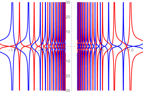
Figure 4: Eigenvalues of $-G^{-1}(0,k)$ for $M/b\simeq 0.0013$ as a function of $k_{x}$. Red and blue curves represent two different sets of eigenvalues. This corresponds to an effective band structure of the topological Hamiltonian of this system, which captures the same topological structure of the original system. This figure also agrees qualitatively with the density plot of spectral densities in the $\omega$-$k_{x}$ plane of the original system. Figure taken from Liu:2018djq .

In the following we summarise the properties for the Green’s function in the three phases.

• In all the three phases, when $k_{z}$ is not zero, the zero frequency retarded Green’s function is real and does not have an imaginary part.

• In the topologically trivial phase, the near horizon geometry guarantees that for all values of $k_{x},k_{y},k_{z}\neq 0$, the retarded Green’s function is real. The pole stays at $k_{x}=k_{y}=k_{z}=0$ as this is a partially gapped trivial semimetal phase.

• For the critical solution, we find that two branches of eigenvalues have peaks in the imaginary part at $k_{x}=k_{y}=0$ and the other two are still small for all $k_{x},k_{y}$.

• Different from the weakly coupled NLSMs, for the holographic NLSM phase, the system has multiple and discrete Fermi surfaces at a set of values of $k_{F}^{i}=\sqrt{k_{x}^{2}+k_{y}^{2}}$ and $k_{z}=0$, $\omega\to 0$, which are closed nodal loops in the $k_{x}$-$k_{y}$ plane. This feature reflects the strong coupling effect of the holographic system. At each nodal line momentum, there is a sharp peak (which becomes a pole at $\omega=0$) in the imaginary part of two eigenvalues of the Green’s function and the imaginary part of the other two eigenvalues are very small indicating that the other two are gapped at this momentum. This different behavior in the $k_{z}$ and $k_{x}$, $k_{y}$ directions are partially caused by the IR Lifshitz geometry.

• Each pair of adjacent nodal lines come from opposite sets of two bands Liu:2018djq . The interval between two adjacent nodal lines gets larger as $k_{F}$ increases. The position of $k_{F}$ of each branch of nodal line decreases as $M/b$ increases and reaches zero at the quantum critical point. The left plot in Fig. 5 shows the value of one branch of $k_{F}^{i}$ as a function of $M/b$. For each branch of nodal lines, we find that the dispersion in both the $k_{z}$ and $k_{x}$ directions are almost linear. The right plot in Fig. 5 shows the dispersion in the $k_{x}$ direction of one branch of nodal lines at $M/b\simeq 0.0013$. A figure taken from Liu:2018djq showing the fermion spectral structure could be found in Fig. 4. More details about the fermion spectral functions and topological invariants of this system could be found in Liu:2018djq .

The spectral function behavior confirms that the topological phase corresponds to a NLSM with multiple nodal lines and the critical and trivial solutions correspond to trivial semimetals. Strong coupling effect produces more complicated topological structures in the NLSM phase. Nontrivial topological invariants could be obtained in the holographic NLSM phase from the dual Green functions Liu:2018djq using the topological Hamiltonian method developed in wang-prx . Moreover, in the holographic NLSM phase as the subleading order of $\phi$ grows bigger the radius of the nodal line circle becomes smaller. This confirms that small perturbations would not gap the system while only making the Fermi nodal circle bigger or smaller.

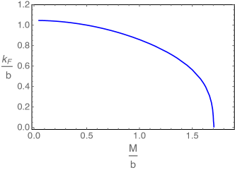
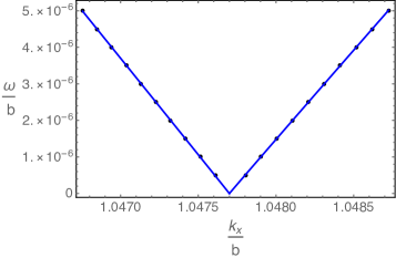
Figure 5: Left: The Femi momentum $k_{F}=\sqrt{k_{x}^{2}+k_{y}^{2}}$ in the holographic NLSMs for $k_{z}=0$. In the critical point or the trivial phase, there is no Fermi surface at finite $k$ and the pole is located at $k=\omega=0$. Right: An example of dispersion relation. For $M/b\simeq 0.0013$, the best fitting curves for the poles are almost linear in $k_{F}-k_{x}$, i.e. for $k_{x}<k_{F}$, $\omega\simeq 0.005(1.0477-k_{x})^{0.998}$; while for $k_{x}>k_{F}$, $\omega\simeq 0.005(k_{x}-1.0477)^{0.994}$.

4 Topological structure in the solution space

In the bulk there is an intrinsic topological structure for this system from the near horizon configurations of the matter fields $B_{ab}$ and $\Phi$.

The near horizon leading order behavior of $B$ and $\phi$ are determined by their IR conformal dimensions $\delta_{\pm}^{B,\phi}$ in the backreacted geometry. As $r^{-\delta_{+}^{B,\phi}}$ is too divergent in the IR, we have $B,\phi\sim c_{B,\phi}r^{-\delta_{-}^{B,\phi}}$. One crucial observation is that with the interaction term between $B$ and $\phi$, $c_{B}$ and $c_{\phi}$ cannot both be nonzero simultaneously. This divided the solutions into three categories: $c_{\phi}=0$ while $c_{B}\neq 0$ corresponding to the topologically nontrivial semimetal solution, $c_{B}=0$ while $c_{\phi}\neq 0$ corresponding to the trivial phase and $c_{\phi}=c_{B}=0$ corresponding to the critical phase where near horizon solutions are subleading terms. In other words, the interaction term always changes the IR scaling dimension of at least one of the fields and it is not possible to keep both scaling dimensions unchanged. Note that this structure is still true with the presence of $\lambda_{1}\phi^{4}$ term where $\phi$ is at most $O(1)$ at leading order and we can substitute $c_{\phi}r^{-\delta_{-}^{\phi}}$ with $c_{\phi}$ in this case.

This structure indicates that when we have a NLSM solution, we cannot find a small perturbation in the IR with $\phi$ at $\phi\sim c_{\phi}r^{-\delta_{-}^{\phi}}$ or $c_{\phi}$ in the case with $\lambda_{1}\phi^{4}$ term, which could (partially) gap the semimetal. This means that the interaction between $B$ and $\phi$ at IR is the intrinsic reason that the nodal line solution is topological. The topological NLSM phase could only become partially gapped after a quantum phase transition passing through the critical point where the nodal line becomes a nodal point.

4.1 A general framework

This holographic NLSM shares the same mathematical structure as the holographic WSM Landsteiner:2015pdh . We propose that there exists a general framework in holography to produce strongly coupled topological gapless states and the key ingredients of the holographic topological structure are:

• A holographic system with at least two interacting fields, with one corresponding to a mass operator, and the other corresponding to an operator that deforms the topology of the Fermi surface, which we denote as $\phi$ and $A$ for illustration. The IR interaction between the two operators produces the topological structure of the solution space in the bulk.

• At the horizon there are three types of solutions: $A$ (or $\phi$) is nonzero at leading order with $r^{-\delta_{-}^{A,\phi}}$ while $\phi$ (or $A$) is at subleading order sourced by $A$ (or $\phi$) and a critical solution with two fields both at subleading order sourcing each other. The fact that $A$ and $\phi$ cannot both be at leading order with $r^{-\delta_{-}^{A,\phi}}$ at the horizon implies that the semimetal phase cannot be gapped by small perturbations.

We expect that a general holographic topological semimetal state shares the properties above. It is expected to be able to describe topological gapped states of matter after introducing bulk fields dual to boundary gapped operators. As there is an intrinsic bulk topological structure for the system that does not require any knowledge of the dual fermion spectral functions, it is possible that this framework would shed light on a better understanding of the deeper organizational principles of strongly coupled topological gapless states of matter and predict new kinds of strongly coupled topological semimetal states.

Appendix A Equations of motion

The equations of motion for the action in the main text are

$$R_{ab}-\frac{1}{2}g_{ab}(R+12)-T_{ab} = 0\,,$$ (18)

$$\nabla_{b}\mathcal{F}^{ba}+2\alpha\epsilon^{abcde}F_{bc}\mathcal{F}_{de} = 0\,,$$ (19)

$$\nabla_{b}F^{ba}+\alpha\epsilon^{abcde}(F_{bc}F_{de}+\mathcal{F}_{bc}\mathcal{F}_{de})~{}~{}~{}~{}~{}~{}$$

$$-iq_{1}\big{(}\Phi^{*}D^{a}\Phi-(D^{a}\Phi)^{*}\Phi\big{)}-\frac{iq_{2}}{\eta}\big{(}B_{ca}^{*}\mathcal{D}^{[b}B^{ca]}-(\mathcal{D}^{[b}B^{ca]})^{*}B_{ca}\big{)} = 0\,,$$ (20)

$$D_{a}D^{a}\Phi-\partial_{\Phi^{*}}V_{1}-\lambda\Phi B_{ab}^{*}B^{ab} = 0\,,$$ (21)

$$\frac{1}{\eta}\mathcal{D}^{a}\mathcal{D}_{[a}B_{bc]}-m_{2}^{2}B_{ab}-\lambda\Phi^{*}\Phi B_{ab} = 0\,,$$ (22)

where

$$T_{ab} = \frac{1}{2}\Big{[}\mathcal{F}_{ac}\mathcal{F}_{b}^{~{}c}-\frac{1}{4}g_{ab}\mathcal{F}^{2}\Big{]}+\frac{1}{2}\Big{[}F_{ac}F_{b}^{~{}c}-\frac{1}{4}g_{ab}F^{2}\Big{]}+\frac{1}{2}\big{(}(D_{a}\Phi)^{*}D_{b}\Phi+(D_{b}\Phi)^{*}D_{a}\Phi\big{)}$$

$$+(m_{2}^{2}+\lambda|\Phi|^{2})(B_{ac}^{*}B_{b}^{~{}c}+B_{bc}^{*}B_{a}^{~{}c})+\frac{1}{2\eta}\big{(}(\mathcal{D}_{[a}B_{cd]})^{*}\mathcal{D}_{[b}B^{cd]}+(\mathcal{D}_{[b}B_{cd]})^{*}\mathcal{D}_{[a}B^{cd]}\big{)}$$

$$-\frac{1}{6\eta}(\mathcal{D}_{[m}B_{cd]})^{*}(\mathcal{D}_{[m}B^{cd]})g_{ab}-\frac{1}{2}\Big{(}(D_{c}\Phi)^{*}(D^{c}\Phi)+V_{1}+V_{2}+\lambda|\Phi|^{2}B_{cd}^{*}B^{cd}\Big{)}g_{ab}\,.$$

In this system, the scalar and the two form fields both have sources at the boundary, therefore for the system to be normalizable at the boundary and without loss of generality we choose the conformal dimension for the source of the dual mass term and the $\bar{\psi}\gamma^{\mu\nu}\psi$ term in (1) to be 1. Thus the massive scalar and 2-form fields in the bulk have the values for the mass to be $m_{1}^{2}=-3$ and $m_{2}^{2}=1$. Furthermore, for simplicity, we set $q_{1}=q_{2}=1$, $\lambda=1$, $\lambda_{1}=0.1$ and $\eta=1.$

After a variation of the total action with respect to the gauge fields, we can obtain the dual consistent currents and they satisfy

$$\partial_{\mu}J^{\mu}_{\text{{con}}} = 0\,,$$

$$\partial_{\mu}J^{\mu}_{5\text{{con}}} = \lim_{r\to\infty}\sqrt{-g}\bigg{(}-\frac{\alpha}{3}\epsilon^{r\alpha\beta\rho\sigma}(F_{\alpha\beta}F_{\rho\sigma}+\mathcal{F}_{\alpha\beta}\mathcal{F}_{\rho\sigma})+iq_{1}\Big{[}\Phi^{*}(D^{r}\Phi)-\Phi(D^{r}\Phi)^{*}\Big{]}+$$

$$~{}~{}~{}~{}~{}~{}~{}~{}~{}+\frac{iq_{2}}{\eta}\big{(}B_{\mu\nu}^{*}\mathcal{D}^{[r}B^{\mu\nu]}-(\mathcal{D}^{[r}B^{\mu\nu]})^{*}B_{\mu\nu}\big{)}\bigg{)}+\text{c.t.}\,.$$

Here we have not explicitly shown the counterterm for simplicity and the above conservation can be further simplified in the radial gauge. The point is that the last two terms contribute only when the non-normalisable mode of the scalar filed or two-from field is switched on and it is straightforward to see that the above identities are of the same structure of the weakly coupled theory (3, 4). Thus this holographic model is expected to go beyond the weakly coupled theory to a strongly coupled nodal line semimetal model.

A.1 Zero temperature

With the ansatz of the zero temperature solution in the main text the corresponding equations of motion are

$$\frac{f^{\prime\prime}}{f}-\frac{u^{\prime\prime}}{u}+\frac{f^{\prime}u^{\prime}}{2fu}-\frac{u^{\prime 2}}{2u^{2}}+\frac{4}{f^{2}}\bigg{(}\frac{B^{\prime 2}}{\eta}+\frac{\lambda B^{2}\phi^{2}}{u}+\frac{m_{2}^{2}B^{2}}{u}\bigg{)} = 0\,,$$

$$\frac{\phi^{\prime 2}}{2}+\frac{6}{u}-\frac{u^{\prime}}{u}\bigg{(}\frac{f^{\prime}}{f}+\frac{u^{\prime}}{4u}\bigg{)}+\frac{B^{\prime 2}}{\eta f^{2}}-\frac{\phi^{2}}{2u}\bigg{(}m_{1}^{2}+\frac{\lambda_{1}}{2}\phi^{2}\bigg{)}-\frac{f^{\prime 2}}{4f^{2}}-\frac{B^{2}}{uf^{2}}\bigg{(}m_{2}^{2}+\lambda\phi^{2}\bigg{)} = 0\,,$$

$$\phi^{\prime\prime}+\left(\frac{3u^{\prime}}{2u}+\frac{f^{\prime}}{f}\right)\phi^{\prime}-\big{(}m_{1}^{2}+\lambda_{1}\phi^{2}+\frac{2\lambda B^{2}}{f^{2}}\big{)}\frac{\phi}{u} = 0\,,$$

$$\frac{B^{\prime\prime}}{\eta}+\frac{B^{\prime}}{\eta}\bigg{(}\frac{3u^{\prime}}{2u}-\frac{f^{\prime}}{f}\bigg{)}-\frac{B}{u}\big{(}m_{2}^{2}+\lambda\phi^{2}\big{)} = 0\,.$$

Close to the boundary $r\to\infty$, we have the following boundary behavior of the fields

$$u = r^{2}-2b^{2}-\frac{M^{2}}{3}+\Big{(}\frac{4b^{4}+2\lambda b^{2}M^{2}+M^{4}}{9}+\frac{\lambda_{1}M^{4}}{6}\Big{)}\frac{\ln r}{r^{2}}+\frac{u_{2}}{r^{2}}+\cdots\,,$$ (23)

$$f = r^{2}-\frac{M^{2}}{3}+\Big{(}\frac{4b^{4}+2\lambda b^{2}M^{2}+M^{4}}{9}+\frac{\lambda_{1}M^{4}}{6}\Big{)}\frac{\ln r}{r^{2}}+\frac{f_{2}}{r^{2}}+\cdots\,,$$ (24)

$$\phi = \frac{M}{r}+\Big{(}-\frac{M^{3}}{3}-\frac{\lambda_{1}M^{3}}{2}-b^{2}M\lambda\Big{)}\frac{\ln r}{r^{3}}+\frac{\phi_{2}}{r^{3}}+\cdots\,,$$ (25)

$$B = br+\Big{(}2b^{3}-\frac{\lambda bM^{2}}{2}\Big{)}\frac{\ln r}{r}+\frac{b_{2}}{r}+\cdots\,,$$ (26)

with $f_{2}=\frac{1}{144}\big{(}56b^{4}+48bb_{2}+14M^{4}-72u_{2}+4b^{2}M^{2}(4+7\lambda)+9M^{4}\lambda_{1}-72M\phi_{2}\big{)}$. Note that we have set the non-physical free parameter related to the shift symmetry $r\to r+c$ in the bulk to be zero in the above expansion. When we extract the boundary data, we should carefully deal with this shift constant.

Radially conserved quantity $\partial_{r}J^{r}=0$ with $J^{r}=\sqrt{u}u^{\prime}f-u^{3/2}f^{\prime}-\frac{4u^{3/2}}{f}BB^{\prime}$. From the near boundary behavior, we have $J^{r}=4f_{2}-4u_{2}+2\lambda M^{2}b^{2}.$ The following scaling symmetry is useful for rescaling the boundary to be asymptotic to standard AdS₅ and $b=1.$
(1) $(x,y)\to a(x,y)\,,~{}~{}(f,B_{xy})\to a^{-2}(f,B_{xy})$ ;
(2) $r\to ar\,,~{}~{}(t,x,y,z)\to a(t,x,y,z)\,,~{}~{}(u,f,B_{xy})\to a^{-2}(u,f,B_{xy})$ .

A.2 Finite temperature

We start from the most general ansatz for the background solutions at finite temperature that are allowed by the symmetry

$$ds^{2} = -udt^{2}+\frac{dr^{2}}{u}+f(dx^{2}+dy^{2})+hdz^{2}\,$$

$$\Phi = \phi(r)\,,$$ (27)

$$B_{xy} = B(r)\,.$$

The equations of motion are

$$\frac{f^{\prime\prime}}{f}-\frac{u^{\prime\prime}}{u}+\frac{f^{\prime}h^{\prime}}{2fh}-\frac{h^{\prime}u^{\prime}}{2hu}+\frac{4}{f^{2}}\bigg{(}\frac{B^{\prime 2}}{\eta}+\frac{\lambda B^{2}\phi^{2}}{u}+\frac{m_{2}^{2}B^{2}}{u}\bigg{)} = 0\,,$$ (28)

$$\frac{f^{\prime\prime}}{f}+\frac{f^{\prime}}{f}\left(\frac{h^{\prime}}{6h}+\frac{2u^{\prime}}{3u}\right)-\frac{f^{\prime 2}}{6f^{2}}-\frac{4}{u}+\frac{2B^{2}}{uf^{2}}\bigg{(}m_{2}^{2}+\lambda\phi^{2}\bigg{)}+~{}~{}~{}~{}$$

$$+\frac{\phi^{2}}{3u}\bigg{(}m_{1}^{2}+\frac{\lambda_{1}\phi^{2}}{2}\bigg{)}+\frac{2B^{\prime 2}}{\eta f^{2}}-\frac{f^{\prime 2}}{6f^{2}}-\frac{h^{\prime}u^{\prime}}{6hu}+\frac{\phi^{\prime 2}}{3} = 0\,,$$ (29)

$$\frac{\phi^{\prime 2}}{2}+\frac{6}{u}-\frac{u^{\prime}}{2u}\bigg{(}\frac{f^{\prime}}{f}+\frac{h^{\prime}}{2h}\bigg{)}-\frac{f^{\prime}h^{\prime}}{2fh}+\frac{B^{\prime 2}}{\eta f^{2}}-\frac{\phi^{2}}{2u}\bigg{(}m_{1}^{2}+\frac{\lambda_{1}}{2}\phi^{2}\bigg{)}~{}~{}~{}~{}$$

$$-\frac{f^{\prime 2}}{4f^{2}}-\frac{B^{2}}{uf^{2}}\bigg{(}m_{2}^{2}+\lambda\phi^{2}\bigg{)} = 0\,,$$ (30)

$$\phi^{\prime\prime}+\left(\frac{f^{\prime}}{f}+\frac{h^{\prime}}{2h}+\frac{u^{\prime}}{u}\right)\phi^{\prime}-\bigg{(}m_{1}^{2}+\frac{2\lambda B^{2}}{f^{2}}+\lambda_{1}\phi^{2}\bigg{)}\frac{\phi}{u} = 0\,,$$ (31)

$$\frac{B^{\prime\prime}}{\eta}+\frac{B^{\prime}}{\eta}\bigg{(}\frac{u^{\prime}}{u}+\frac{h^{\prime}}{2h}-\frac{f^{\prime}}{f}\bigg{)}-\frac{B}{u}\big{(}m_{2}^{2}+\lambda\phi^{2}\big{)} = 0\,.$$ (32)

Note that the ansatz (A.2) is invariant under two independant transformations

$$(t,x,y,z,r)\to(a^{-2\alpha-\beta}t,a^{\alpha}x,a^{\alpha}y,a^{\beta}z,a^{2\alpha+\beta}r),~{}~{}(u,f,h,\phi,B)\to(a^{4\alpha+2\beta}u,a^{-2\alpha}f,a^{-2\beta}h,\phi,a^{-2\alpha}B)$$

with constant $a$ and arbitrary $\alpha$ and $\beta$. The corresponding two Noether currents (radially conserved quantities) are $J_{1}^{r}=fh^{3/2}\big{(}u/h\big{)}^{\prime}$ and $J_{2}^{r}=\frac{fuh^{\prime}}{\sqrt{h}}-u\sqrt{h}f^{\prime}-\frac{4u\sqrt{h}BB^{\prime}}{f}$. From the near horizon behavior of the fields one concludes that $J_{1}^{r}=Ts$ with $s$ the entropy of the system. At zero temperature, we have $J_{1}^{r}=0$ which leads to $h=u$ and the ansatz (A.2) is reduced to the zero temperature ansatz in the main text and this confirms that the ansatz made for the zero temperator background is the most generic one. The sencond Noether current $J_{2}^{r}$ reduced to the one discussed in the subsection for zero temperature.

Appendix B Free energy

For each value of $M/b$ from the boundary, there is only one bulk solution, nevertheless we can compute the free energy of this system to see whether the phase transition is a continuous one. To compute the free energy, we need to be careful with the boundary counterterms. The total action is

$$S_{\text{ren}}=S+S_{\text{GH}}+S_{\text{c.t.}}$$ (33)

with the Gibbons-Hawking boundary term $S_{\text{GH}}=\int_{r=r_{\infty}}d^{4}x\sqrt{-\gamma}(2K)$ and the counterterms

$$S_{\text{c.t.}} = \int_{r=r_{\infty}}d^{4}x\sqrt{-\gamma}\bigg{(}-6-|\Phi|^{2}+|B_{\mu\nu}|^{2}+\frac{1}{2}(\log r^{2})\bigg{[}\frac{1}{4}\mathcal{F}^{2}+\frac{1}{4}F^{2}+|D_{\mu}\Phi|^{2}+$$

$$~{}~{}~{}~{}+\bigg{(}\frac{1}{3}+\frac{\lambda_{1}}{2}\bigg{)}|\Phi|^{4}+\frac{1}{3\eta}\big{(}\mathcal{D}_{[\mu}B_{\alpha\beta]}\big{)}^{*}\big{(}\mathcal{D}^{[\mu}B^{\alpha\beta]}\big{)}-|B_{\mu\nu}|^{4}+\lambda|\Phi|^{2}|B_{\mu\nu}|^{2}\bigg{]}\bigg{)}$$

where $\gamma_{\mu\nu}$ is the metric induced by $g_{ab}$ on the boundary via $\gamma_{ab}=g_{ab}-n_{a}n_{b}$ where $n_{a}$ is outward pointing unit normal vector of the boundary. $K=\gamma^{ab}\nabla_{a}n_{b}$ is the trace of the extrinsic curvature with respect to the metric at the boundary.

From the $zz$ component of the Einstein equation (18), we have $R_{zz}-\frac{1}{2}g_{zz}\mathcal{L}=0$. Thus the bulk on-shell action is a total derivative

$$S=\int d^{4}xdr\sqrt{-g}\mathcal{L}=-\int d^{4}x\int_{0}^{r_{\infty}}dr\big{[}fu^{1/2}u^{\prime}\big{]}^{\prime}.$$ (34)

Taking into account the boundary terms and performing a Wick rotation, the free energy density can be obtained as

$$\frac{\Omega}{V}=\frac{7}{9}b^{4}-\frac{4bb_{2}}{3}+\frac{7M^{4}}{36}-3u_{2}+\frac{5+8\lambda}{9}b^{2}M^{2}-2M\phi_{2}\,.$$ (35)

The stress tensor for the dual field theory can be calculated as

$$T_{\mu\nu}=2(K_{\mu\nu}-\gamma_{\mu\nu}K)+\frac{2}{\sqrt{-\gamma}}\frac{\delta S_{\text{c.t.}}}{\delta\gamma^{\mu\nu}}\,.$$ (36)

The total energy density is $\epsilon=\lim_{r\to\infty}\sqrt{-\gamma}\langle T^{0}_{0}\rangle=\frac{7}{9}b^{4}-\frac{4bb_{2}}{3}+\frac{7M^{4}}{36}-3u_{2}+\frac{5+8\lambda}{9}b^{2}M^{2}-2M\phi_{2}$, thus $\frac{\Omega}{V}=\epsilon.$

The free energy can be found in the main text and we conclude that the system is smooth when it crosses the phase transition.

Appendix C Probe limit

The simplest way to solve the system is to consider the probe limit $\kappa/L^{3/2}\ll 1$. However, the probe limit for the nodal line semimetal system is not well defined near the horizon and even with another set of scaling dimensions where the probe limit is well defined near the horizon it is not valid near the critical point. For the axial vector field in the holographic Weyl semimetal, the probe limit is a good limit for the same scaling dimensions of operators dual to $A_{z}$ and $B_{xy}$ except near the critical point.

In the probe limit, we assume that the Newton coupling constant is very small so that the backreaction to the geometry could be ignored. We need to check if the probe limit is satisfied for a given solution of $B$ and $\phi$. The equations of motion for $B$ and $\phi$ in the $AdS_{5}$ background is

$$B^{\prime\prime}+\frac{B^{\prime}}{r}-\frac{m_{b}^{2}B}{r^{2}}-\frac{\eta B\phi^{2}}{2r^{2}}=0\,,$$ (37)

$$\phi^{\prime\prime}+\frac{5\phi^{\prime}}{r}-\frac{m_{\phi}^{2}\phi}{r^{2}}-\frac{\eta B^{2}\phi}{r^{6}}=0\,.$$ (38)

We have to make sure that the source term of $B$ and $\phi$ at both the boundary and the horizon are small enough not to cause too much backreaction. In the probe limit, the IR scaling dimention of $B$ and $\phi$ is the same as the UV scaling. Thus it seems that there is only one scaling dimenion that we can use, which is zero for both fields, otherwise, the fields either backreact too much at the horizon or too much at the boundary. In this way, the two fields contribute at $\kappa^{2}$ order compared to the background and when $\kappa\to 0$ the probe limit is a physically well defined limit for finite solutions.

Let us focus on $m_{\phi}=0$ and $m_{B}=2$. There are three types of near horizon solutions The first solution is

$$\phi \simeq \phi_{0}+\phi_{1}(\phi_{0},b_{1})r^{\sqrt{16+2\lambda\phi_{0}^{2}}-4}+\cdots,$$ (39)

$$B_{xy} \simeq b_{1}r^{4+\lambda\phi_{0}^{2}/2}+\cdots,$$ (40)

where $b_{1}$ is a tuning parameter and the second solution is

$$\phi \simeq \phi_{1}r^{\sqrt{4+\lambda b_{0}^{2}}-2}+\cdots,$$ (41)

$$B_{xy} \simeq b_{0}r^{2}+b_{1}(b_{0},\phi_{1})r^{2(\sqrt{4+\lambda b_{0}^{2}}-1)}$$ (42)

where $\phi_{1}$ is a tuning parameter. The critical solution is $B_{xy}=1/\sqrt{2}r^{2}\phi$ and the critical point is $M/b=\sqrt{2}$. This is a special property of the probe limit at the critical point, which is also true for the holographic Weyl semimetal model at the probe limit. Flowing this geometry to the boundary we find that at the boundary, though the scaling dimension of $B$ and $\phi$ guarantees that free $B$ or $\phi$ does not have backreaction in the probe limit, the interaction at the UV makes both $B$ and $\phi$ more divergent than their scaling dimensions, which means that it cannot flow to asymptotic $AdS_{5}$ solutions.

To solve this problem and make the probe limit well defined, we introduce another scalar field $\lambda$ which mediates the interaction between $B$ and $\phi$ and choose a scaling dimension for $\lambda$ so that the interaction term is not important in the UV so that the probe limit is still valid. We change the interaction term of $\phi$ and $B$ to $\lambda^{2}B^{2}\phi^{2}$ and introduce the kinetic term for $\lambda$ in the action with a relative minus sign. The equations of motion now become

$$B^{\prime\prime}+\frac{B^{\prime}}{r}-\frac{m_{b}^{2}B}{r^{2}}-\frac{\eta\lambda^{2}B\phi^{2}}{2r^{2}}=0\,,$$ (43)

$$\phi^{\prime\prime}+\frac{5\phi^{\prime}}{r}-\frac{m_{\phi}^{2}\phi}{r^{2}}-\frac{\eta\lambda^{2}B^{2}\phi}{r^{6}}=0\,,$$ (44)

$$\lambda^{\prime\prime}+\frac{5\lambda^{\prime}}{r}-\frac{m_{\lambda}\lambda}{r^{2}}-\frac{V_{0}\lambda^{3}}{r^{2}}+\frac{\eta\lambda B^{2}\phi^{2}}{r^{6}}=0\,,$$ (45)

where $B$ denotes $B_{xy}$. We choose $m_{\lambda}^{2}=-3$ so that the interaction at the UV is not important. For the interaction to be not important in the IR we introduce a $\lambda^{4}$ potential term for the $\lambda$ scalar.

The near horizon boundary conditions now have a new field $\lambda=\sqrt{3/V_{0}}+\cdots$ where the subleading terms in $\lambda$ depends on the phase of the solution. For the other two fields, the near horizon boundary condition does not change except to substitute $\eta$ with $3\eta/v_{0}$. Flowing these solutions to the boundary and we could also get a valid probe limit system with three different types of solutions. This probe limit is well defined for most of the parameter regime. However, near the critical point the probe limit becomes subtle because the solutions become larger and larger near the boundary when getting more and more close to the critical point. Thus considering backreactions is a better and more physical choice, and here we do not elaborate more on this probe limit.

References

- (1) E. Witten, Three Lectures On Topological Phases Of Matter, Riv. Nuovo Cim. 39, no. 7, 313 (2016) [arXiv:1510.07698].
- (2) C.-K. Chiu, J. C.Y. Teo, A. P. Schnyder, S. Ryu, Classification of topological quantum matter with symmetries, Rev. Mod. Phys. 88, 035005 (2016) [arXiv:1505.03535].
- (3) W. Witczak-Krempa, M. Knap and D. Abanin, Interacting Weyl semimetals: characterization via the topological Hamiltonian and its breakdown, Phys. Rev. Lett. 113 (2014) 136402 [arXiv:1406.0843].
- (4) J. Liu, L. Balents, Correlation and transport phenomena in topological nodal-loop semimetals, Phys. Rev. B 95, 075426 (2017) [arXiv:1609.05529].
- (5) J. Zaanen, Y. W. Sun, Y. Liu and K. Schalm, Holographic Duality in Condensed Matter Physics, Cambridge University Press, 2015.
- (6) M. Ammon and J. Erdmenger, Gauge/gravity duality: Foundations and applications, Cambridge University Press, 2015.
- (7) S. A. Hartnoll, A. Lucas and S. Sachdev, Holographic quantum matter, [arXiv:1612.07324], MIT Press, 2017.
- (8) C. Hoyos-Badajoz, K. Jensen and A. Karch, A Holographic Fractional Topological Insulator, Phys. Rev. D 82, 086001 (2010) [arXiv:1007.3253].
- (9) C. Kristjansen and G. W. Semenoff, The D3-probe-D7 brane holographic fractional topological insulator, JHEP 1610, 079 (2016) [arXiv:1604.08548].
- (10) Y. Seo, G. Song and S. J. Sin, Strong Correlation Effects on Surfaces of Topological Insulators via Holography, Phys. Rev. B 96, no. 4, 041104 (2017) [arXiv:1703.07361].
- (11) M. Fujita, W. Li, S. Ryu and T. Takayanagi, Fractional Quantum Hall Effect via Holography: Chern-Simons, Edge States, and Hierarchy, JHEP 0906, 066 (2009) [arXiv:0901.0924].
- (12) O. Bergman, N. Jokela, G. Lifschytz and M. Lippert, Quantum Hall Effect in a Holographic Model, JHEP 1010, 063 (2010) [arXiv:1003.4965].
- (13) K. Landsteiner, Y. Liu and Y. W. Sun, Quantum phase transition between a topological and a trivial semimetal from holography, Phys. Rev. Lett. 116, no. 8, 081602 (2016) [arXiv:1511.05505].
- (14) K. Landsteiner, Y. Liu and Y. W. Sun, Odd viscosity in the quantum critical region of a holographic Weyl semimetal, Phys. Rev. Lett. 117, no. 8, 081604 (2016) [arXiv:1604.01346].
- (15) C. Copetti, J. Fernandez-Pendas and K. Landsteiner, Axial Hall effect and universality of holographic Weyl semi-metals, JHEP 1702, 138 (2017) [arXiv:1611.08125].
- (16) M. Ammon, M. Heinrich, A. Jimenez-Alba and S. Moeckel, Phys. Rev. Lett. 118, no. 20, 201601 (2017) [arXiv:1612.00836].
- (17) K. Landsteiner and Y. Liu, The holographic Weyl semi-metal, Phys. Lett. B 753, 453 (2016) [arXiv:1505.04772].
- (18) G. Grignani, A. Marini, F. Pena-Benitez and S. Speziali, AC conductivity for a holographic Weyl Semimetal, JHEP 1703, 125 (2017) [arXiv:1612.00486].
- (19) A. A. Burkov, M. D. Hook and L. Balents, Topological nodal semimetals, Phys. Rev. B 84, 235126 (2011) [arXiv:1110.1089].
- (20) C. Fang, H. Weng, X. Dai and Z. Fang, Topological nodal line semimetals, Chin. Phys. B 25, 117106 (2016) [arXiv:1609.05414].
- (21) R. Alvares, C. Hoyos and A. Karch, An improved model of vector mesons in holographic QCD, Phys. Rev. D 84, 095020 (2011) [arXiv:1108.1191].
- (22) S. Grozdanov and N. Poovuttikul, Generalised global symmetries and magnetohydrodynamic waves in a strongly interacting holographic plasma, arXiv:1707.04182.
- (23) D. M. Hofman and N. Iqbal, Generalized global symmetries and holography, SciPost Phys. 4, 005 (2018) [arXiv:1707.08577].
- (24) R. G. Cai and R. Q. Yang, Paramagnetism-Ferromagnetism Phase Transition in a Dyonic Black Hole, Phys. Rev. D 90, no. 8, 081901 (2014) [arXiv:1404.2856].
- (25) N. Iqbal, H. Liu and M. Mezei, Quantum phase transitions in semilocal quantum liquids, Phys. Rev. D 91, no. 2, 025024 (2015) [arXiv:1108.0425].
- (26) A. Donos and S. A. Hartnoll, Interaction-driven localization in holography, Nature Phys. 9, 649 (2013) [arXiv:1212.2998].
- (27) S. A. Hartnoll and L. Huijse, Fractionalization of holographic Fermi surfaces, Class. Quant. Grav. 29, 194001 (2012) [arXiv:1111.2606].
- (28) Y. Liu, K. Schalm, Y. W. Sun and J. Zaanen, Bose-Fermi competition in holographic metals, JHEP 1310, 064 (2013) [arXiv:1307.4572].
- (29) N. Iqbal and H. Liu, Real-time response in AdS/CFT with application to spinors, Fortsch. Phys. 57, 367 (2009) [arXiv:0903.2596].
- (30) H. Liu, J. McGreevy and D. Vegh, Non-Fermi liquids from holography, Phys. Rev. D 83, 065029 (2011) [arXiv:0903.2477].
- (31) M. Cubrovic, J. Zaanen and K. Schalm, String Theory, Quantum Phase Transitions and the Emergent Fermi-Liquid, Science 325, 439 (2009) [arXiv:0904.1993].
- (32) Y. Liu and Y. W. Sun, Topological invariants for holographic semimetals, JHEP 1810, 189 (2018) [arXiv:1809.00513].
- (33) Z. Wang and S. C. Zhang, Topological Invariants and Ground-State Wave Functions of Topological Insulators on a Torus, Phys. Rev. X 4, no. 1, 011006 (2014) [arXiv:1308.4900].