KRISM — Krylov Subspace-based Optical Computing of Hyperspectral Images
Abstract.
We present an adaptive imaging technique that optically computes a low-rank approximation of a scene’s hyperspectral image, conceptualized as a matrix. Central to the proposed technique is the optical implementation of two measurement operators: a spectrally-coded imager and a spatially-coded spectrometer. By iterating between the two operators, we show that the top singular vectors and singular values of a hyperspectral image can be adaptively and optically computed with only a few iterations. We present an optical design that uses pupil plane coding for implementing the two operations and show several compelling results using a lab prototype to demonstrate the effectiveness of the proposed hyperspectral imager.
1. Introduction
Hyperspectral images (HSIs) capture light intensity of a scene as a function of space and wavelength and have been used in numerous vision [Pan et al., 2003; Tarabalka et al., 2010; Kim et al., 2012], geo-science and remote sensing applications [Cloutis, 1996; Harsanyi and Chang, 1994]. Traditional approaches for hyperspectral imaging, including tunable spectral filters and pushbroom cameras, rely on sampling the HSI, i.e., measuring the photon counts in each spatio-spectral voxel. When imaging at high-spatial and spectral resolutions, the amount of light in a voxel can be quite small, thus requiring long exposures to mitigate the effect of noise.
HSIs are often endowed with rich structures that can be used to alleviate the challenges faced by traditional imagers. For example, natural scenes are often comprised of a few materials of distinct spectra and further, illumination of limited spectral complexity [Parkkinen et al., 1989; Lee et al., 2000]. This implies that the collection of spectral signatures observed at various locations in a scene lies close to a low-dimensional subspace. Instead of sampling the HSI of the scene one spatio-spectral voxel at a time, we can dramatically speed-up acquisition and increase light throughput by measuring only projections on this low-dimensional subspace. However, such a measurement scheme requires a priori knowledge of the scene since this subspace is entirely scene dependent. This paper introduces an optical computing technique that identifies this subspace using an iterative and adaptive sensing strategy and constructs a low-rank approximation to the scene’s HSI.
The proposed imager senses a low-rank approximation of a HSI by optically implementing the so-called Krylov subspace method [Golub and Kahan, 1965]. We show that this requires two operators: a spatially-coded spectrometer and a spectrally-coded spatial imager; when we interpret the HSI as a 2D matrix, these two operators correspond to left and right multiplication of the matrix with a vector. The two operators are subsequently used in an iterative and adaptive imaging procedure whose eventual output is a low-rank approximation to the HSI. The proposed imager is adaptive, i.e., the measurement operator used to probe the scene’s HSI at a given iteration depends on previously made measurements. This is a marked departure from current hyperspectral imaging strategies where the signal model is merely used as a prior for recovery from non-adaptive measurements [Arce et al., 2014].
Contributions.
We propose an optical architecture that we refer to as KRylov subspace-based Imaging and SpectroMetry (KRISM) and make the following three contributions:
-
•
Optical computation of HSIs. We show that optical computing of HSIs to estimate its dominant singular vectors provides significant advantages in terms of increased light throughput and reduced measurement time.
-
•
Coded apertures for resolving space and spectrum. Sensing architectures typically used in spectrometry and imaging are mutually incompatible due to use the of slits in spectral imaging and open apertures in conventional imaging. To mitigate this, we study the effect of pupil plane coding on the HSI and propose a coded aperture design that is capable of simultaneously achieving high spatial and spectral resolutions.
-
•
Optical setup. We design and validate a novel and versatile optical implementation for KRISM that uses a single camera and a single spatial light modulator (SLM) to efficiently implement spatially-coded spectral and spectrally-coded spatial measurements.
The contributions above are supported via an extensive set of simulations as well as real experiments performed using the lab prototype.
Limitation.
The benefits and contributions described above come with a key limitation. Our method is only advantageous if there are a sufficient number of spectral bands and the hyperspectral image is sufficiently low rank. If we only seek to image with very few spectral bands or if the scene is not well approximated by a low-rank model, then the proposed method performs poorly against traditional sensing methods.
2. Prior work
Nyquist sampling of HSIs.
Classical designs for hyperspectral imaging based on Nyquist sampling include the tunable filter — which scans one narrow spectral band at a time, measuring the image associated with spectral bands at each instant — or using a pushbroom camera — which scans one spatial row at a time, measuring the entire spectrum associated with each pixel on the row. Both approaches are time-consuming as well as light inefficient since each captured image wastes a large percentage of light incident on the camera.
Multiplexed sensing.
The problem of reduced light throughput can be mitigated by the use of multiplexing. One of the seminal results in computational imaging is that the use of multiplexing codes including the Hadamard transform can often lead to significant efficiencies either in terms of increased SNR or faster acquisition [Harwit and Sloane, 1979]. This can either be spectral multiplexing [Mohan et al., 2008] or spatial multiplexing [Sun and Kelly, 2009]. While multiplexing mitigates light throughput issues, it does not reduce the number of measurements required. Sensing at high spatial and/or spectral resolution still requires long acquisition times to maintain a high SNR. Fortunately, HSIs have concise signal models that can be exploited to reduce the number of measurements.
Low-rank models for HSIs.
There are many approaches to approximate HSIs using low-dimensional models; this includes group sparsity in transform domain [Rasti et al., 2013], low rank model [Li et al., 2012; Golbabaee and Vandergheynst, 2012], as well as low-rank and sparse model [Waters et al., 2011; Saragadam et al., 2017]. Of particular interest to this paper is the low-rank modeling of HSIs when they are represented as a 2D matrix (See Figure 2). These models have found numerous uses in vision and graphics including color constancy [Finlayson et al., 1994], color displays [Kauvar et al., 2015], endmember detection [Winter, 1999], source separation [Hui et al., 2018], anomaly detection [Saragadam et al., 2017], compressive imaging [Golbabaee and Vandergheynst, 2012] and denoising [Zhao and Yang, 2015]. Chakrabarti and Zickler [2011] also provide empirical justification that HSIs of natural scenes are well represented by low dimensional models.
![[Uncaptioned image]](/html/1801.09343/assets/x3.png)
Compressive hyperspectral imaging.
The low-rank model has also been used for compressive sensing (CS) of HSIs. CS aims to recover a signal from a set of linear measurements that are fewer than its dimensionality [Baraniuk, 2007]. This is achieved by modeling the sensed signal using lower dimensional representations — low-rank matrices being one such example. The technique most relevant to this paper is that of row/column projection [Fazel et al., 2008] where the measurement model is restricted to obtaining row and column projections of a matrix. Given a matrix , and measurement operators , the measurements acquired are of the following form,
When the matrix has a rank , it can be shown that it is sufficient to acquire images and spectral profiles with . In contrast, the method proposed in this paper requires only a number of measurements proportional to the rank of the matrix; however, these measurements are adaptive to the scene. At an increased cost of optical complexity, adaptive sensing promises accurate results with fewer measurements than non-adaptive measurement strategies.
Hyperspectral imaging architectures.
Several architectures have been proposed for CS acquisition of HSIs. The Dual-Disperser Coded Aperture Snapshot Spectral Imager (DD-CASSI) [Gehm et al., 2007] obtains a single image multiplexed in both spatial and spectral domains by dispersing the image with a prism, passing it through a coded aperture, and then recombining with a second prism. In contrast, the Single Disperser CASSI (SD-CASSI) [Wagadarikar et al., 2008] relies on a single prism that performs spatial coding using a binary mask followed by spectral dispersion with a prism. Baek et al. [2017] disperse the image by placing a prism right before an SLR camera. The HSI is then reconstructed by studying the dispersion of color at the edges in the obtained RGB image. Takatani et al. [2017] instead propose a snapshot imager that uses a faced reflectors overlaid with color filters. Various other snapshot techniques have been proposed which rely on space-spectrum multiplexing [Cao et al., 2016; Lin et al., 2014a; Jeon et al., 2016]. While snapshot imagers require only a single image, they often produce HSIs with reduced spatial or spectral resolutions. Data-driven approaches such as overcomplete dictionaries [Lin et al., 2014a] and convolutional neural networks [Choi et al., 2017] partially alleviate the loss in resolution by building priors for the HSI. However, they require complex optimization that can often be time consuming.
Resolution and accuracy of the HSI can be improved by acquiring multiple measurements instead of a single snapshot image. Examples include multiple spatio-spectrally encoded images [Kittle et al., 2010], spatially-multiplexed spectral measurements [Li et al., 2012; Sun and Kelly, 2009] or separate spatial and spectral coding [Lin et al., 2014b]. While multi-measurement techniques overcome spatial and spectral resolution limits, the price is paid in the form of increased number of measurements and hence, reduced time resolution.
Performance of snapshot techniques can be improved by tailoring the spatial masks to a given HSI dataset [Rueda et al., 2016, 2017] or by optimizing spatial masks for sensing a selected subset of spectral bands [Arguello and Arce, 2013]. Optimizing the spatial masks results in increased accuracy, but still requires long reconstruction times. A key insight into the existing methods is that the measurements are either non-adaptive and random, or adapted to a fixed signal class. In contrast, the proposed method is adapted to the specific instance of the signal, requires fewer measurements, and has practically no post-processing for reconstruction. Table 1 compares and contrasts various HS imaging strategies and their relative merits in terms of number of measurements and error in reconstruction. We next discuss the concept of Krylov subspaces for low-rank approximation of matrices, which motivates iterative and adaptive techniques and paves the way to the proposed method.
Krylov subspaces.
Central to the proposed method is a class of techniques, collectively referred to as Krylov subpaces, for estimating singular vectors of matrices. Recall that the singular value decomposition (SVD) of a matrix is given as , where and are orthonormal matrices, referred to as the singular vectors, and is a diagonal matrix of singular values. Krylov subspace methods allow for efficient estimation of the singular values and vectors of a matrix and enjoy two key properties. First, we only need access to the matrix via left and right multiplications with vectors, i.e., we do not need explicit access to the elements of the matrix . Second, the top singular values and vectors of a low-rank matrix can be estimated using a small set of matrix-vector multiplications. These two properties are invaluable when the matrix is very large or when it is implicitly represented using operators or, as is the case in this paper, the matrix is the scene’s HSI and we only have access to optical implementations of the underlying matrix-vector multiplications.
There are many variants of Krylov subspace techniques which differ mainly on their robustness to noise and model mismatch. The techniques in this paper are based on the so-called Lanczos bidiagonalization with full orthogonalization [Golub and Kahan, 1965; Hernandez et al., 2007]. Such iterative operations to reduce the complexity of matrix-vector multiplications have found use in communication theory in the form of reduced-rank filtering [Tian et al., 2005; Ge et al., 2004] and adaptive beam forming [Ge et al., 2006]. Our goal is to leverage the benefits of iterative operations for low-rank approximation of high dimensional optical signals, in particular HSIs.
Optical computing of low-rank signals.
Matrix-vector and matrix-matrix multiplications can often be implemented as optical systems. Such systems have been used for matrix-matrix multiplication [Athale and Collins, 1982], matrix inversion [Rajbenbach et al., 1987], as well as computing eigenvectors [Vijaya Kumar and Casasent, 1981]. Of particular interest to our paper is the optical computing of the light transport operator using Krylov subspace methods [O’Toole and Kutulakos, 2010]. The light transport matrix represents the linear mapping between scene illumination and a camera observing the scene. Each column of the matrix is the image of the scene when only a single illuminant is turned on. Hence, given a vector that encodes the scene illumination, the image captured by the camera is given as . By Helmholtz reciprocity, if we replaced every pixel of the camera by a light source and every illuminant with a camera pixel, then the light transport associated with the reversed illumination/sensing setup is given as . Hence, by co-locating a projector with the camera and a camera with the scene’s illuminants, we have access to both left- and right-multiplication of the light transport matrix with vectors; we can now apply Krylov subspace techniques for optically estimating a low-rank approximation to the light transport matrix. This delightful insight is one of the key results in [O’Toole and Kutulakos, 2010].
This paper proposes a translation of the ideas in [O’Toole and Kutulakos, 2010] to hyperspectral imaging. However, as we will see next, this translation is not straightforward and requires the construction of novel imaging architectures.
3. Optical Krylov Subspaces for Hyperspectral Imaging
In this section, we provide a high-level description of optical computing of HSIs using Krylov subspace methods.
Notation.
We represent HSIs in two different ways:
-
•
— a real-valued function over 2D space and 1D spectrum ,
-
•
— a matrix with rows and columns, such that each column corresponds to the vectorized image at a specific spectrum.
The goal is to optically build the following two operators:
-
•
Spectrally-coded imager — Given a spectral code , we seek to measure the image given as
(1) The image corresponds to a grayscale image of the scene with a camera whose spectral response is .
-
•
Spatially-coded spectrometer — Given a spatial code , we seek to measure a spectral measurement given as
(2) The measurement corresponds to the spectral measurement of the scene, where-in the spectral profile of each pixel is weighted by the corresponding entry in the spatial code .
Since the two operators correspond to left and right multiplication of a vector to the HSI matrix , we can implement any Krylov subspace technique to estimate the top singular vectors and values.
Number of measurements required.
To obtain a rank- approximation of the matrix , we would require at least spatially-coded spectral measurements — each of dimensionality , and spectrally-coded images — each of dimensionality . Hence, the number of measurements required by the approach is proportional to and, over traditional Nyquist sampling, it represents a reduction in measurements by a factor of
| (3) |
For low-rank HSIs, we can envision dramatic reductions in measurements required over Nyquist sampling especially when sensing at high spatial and spectral resolutions (see Table 1).
Challenges in implementing operators and .
Spatially-coded spectral measurements have been implemented in the context of compressive hyperspectral imaging [Sun and Kelly, 2009]. Here, light from a scene is first focused onto an SLM that performs spatial coding, and then directed into a spectrometer. For spectral coding at a high-resolution, we could replace the sensor in a spectrometer with an SLM; subsequently, we can form and measure an image of the coded light using a lens. However, high-resolution spectrometers invariably use a slit aperture that produces a large one-dimensional blur in the spatial image due to diffraction. We show in Section 4 that simultaneous spatio-spectral localization is not possible with either a slit or an open aperture. This leads to the design of optimal binary coded apertures which enable high spectral and spatial resolutions. Subsequently, in Section 6, we present the design of KRISM and validate its performance in Section 7.
4. Coded apertures for simultaneous sensing of space and spectrum
In this section, we introduce an optical system capable of simultaneously resolving space and spectrum at high resolutions.
4.1. Optical setup
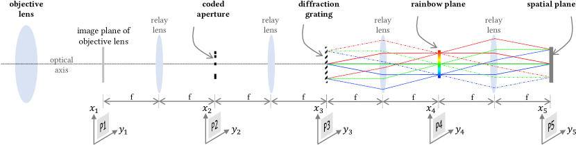
The ideas proposed in this paper rely on the optical setup shown in Figure 19 which is a slight modification of a traditional spectrometer. An objective lens focuses a scene onto its image plane, that we denote as P1. This is followed by two 4 relays with a coded aperture placed on the first pupil plane, P2, and a diffraction grating placed at the plane marked as P3. We are interested in the intensity images formed at the planes marked at the “rainbow plane” P4 and the “spatial plane” P5, and their relationship to the image formed on P1, the coded aperture, and the grating parameters.
We assume that the field formed on the plane P1 is incoherent and, hence, we only need to consider its intensity and how it propagates, and largely ignore its phase. Let be the intensity of the field as a function of spatial coordinates and wavelength . Let be the aperture code placed at the plane P2, be the density (measured in grooves per unit length) of the diffraction grating in P3, and be the focal length of the lenses that form the 4 relays. The hyperspectral field intensity at the plane P4 is given as
| (4) |
where is the scene’s overall spectral content defined as
The intensity field at the spatial plane P5 is given as
| (5) |
where is the 2D spatial Fourier transform of the aperture code , and denotes two-dimensional spatial convolution along and axes. These expressions arise from Fourier optics [Goodman, 2005] and their derivation is provided in the supplemental material.
Image formed at the rainbow plane P4.
A camera with spectral response placed at the rainbow plane would measure
| (6) |
where . Here, the dimensionless term , that scales of the spectrum , indicates the resolving power of the diffraction grating. For example, we used a focal length mm and a grating with groove density grooves/mm for the prototype discussed in Section 6; here, . This implies that the spectrum is stretched by a factor of . Therefore, a nm of the spectrum maps to 30 m, which is about 6-7 pixel-widths on the camera that we used. The key insight this expression provides is that the image is the convolution of the scene’s spectrum — denoted as a 1D image — with the aperture code (see Figure 4). This implies that we can measure the spectrum of the scene, albeit convolved with the aperture code on this plane; this motivates our naming of this plane as the rainbow plane.
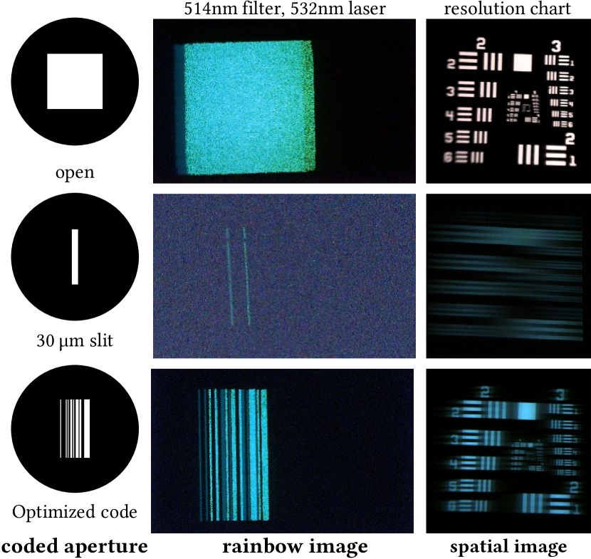
Image at the spatial plane P5.
A camera with the spectral response placed at the spatial plane P5 would measure
| (7) |
is a “spatial image” in that spectral components of the HSI have been integrated out. Hence, we refer to P5 as the spatial plane. Figure 4 shows the image formed at P5 for different choices of the coded apertures, including slits and open apertures.
Implementing KRISM operations.
The derivation above suggests that we get a spatial image of the scene formed at the spatial plane P5 and a spectral profile at the rainbow plane P4. We can therefore build the two operators central to KRISM by coding light on one of the planes while measuring it at the other. For the spectrally-coded imager , we will place an SLM on the rainbow plane P4 while measuring the image, with a camera, at P5. For the spatially-coded spectrometer , we place an SLM on P3 — which is optically identical to P5 — while measuring the image formed at P4.
Effect of the aperture code on the scene’s HSI
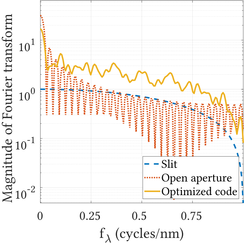
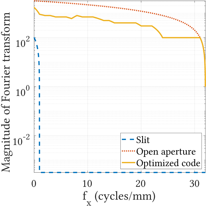
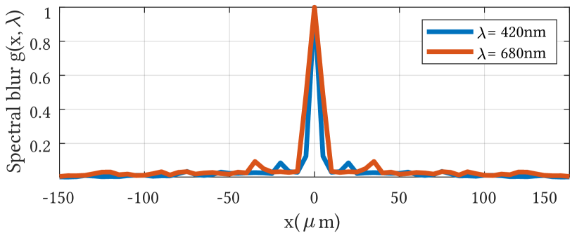
Introducing an aperture code on the plane P2 can be interpreted as distorting the scene’s HSI in two distinct ways. First, a spectral blur is introduced whose point spread function (PSF) is a scaled copy of the aperture code . Second, a spatial blur is introduced for each spectral band whose PSF is the power spectral density (PSD) of the aperture code, suitably scaled. With this interpretation, the images formed on planes P4 and P5 are a spectral and spatial projection, respectively, of this new blurred HSI. Our proposed technique measures a low-rank approximation to this blurred HSI and we can, in principle, deblur it to obtain the true HSI of the scene. However, the spatial and spectral blur kernels may not always be invertible. As we show next, the choice of the aperture is critical and that traditional apertures such as a slit in spectrometry and an open aperture in imaging will not lead to invertible blur kernels.
4.2. Failure of slits and open apertures
We now consider the effect of the traditional apertures used in imaging and spectrometry — namely, an open aperture and a slit, respectively — on the images formed at the rainbow and the spatial planes. Suppose that the aperture code is a box function of width mm and height mm, i.e.,
Its Fourier transform is the product of two sincs
The spatial image is convolved with the PSD scaled by , so the blur observed on it has a spatial extent of units. Suppose that and m, the observed blur is . The rainbow plane image , on the other hand, simply observes a box blur whose spatial extent is . Armed with these expressions, we can study the effect of an open and a slit apertures on the spatial and rainbow images.

Scenario #1 — An open aperture.
Suppose that mm, then we can calculate the spatial blur to be m in both height and width and hence, we can expect a very sharp spatial image of the scene. The blur on the rainbow image has a spread of mm; for relay lenses with focal length mm and grating with groove density grooves/mm, this would be equivalent of a spectral blur of nm. Hence, we cannot hope to achieve high spectral resolution with an open aperture.
Scenario #2 — A slit.
A slit is commonly used in spectrometers; suppose that we use a slit of width m and height mm. Then, we expect to see a spectral blur of nm. The spatial image is blurred along the y-axis by a m blur and along the x-axis by a m blur; effectively, with a m pixel pitch, this would correspond to a 1D blur of 100 pixels. In essence, the use of a slit leads to severe loss in spatial resolution.
Figure 4 shows images formed at the rainbow and spatial planes for various aperture codes. This validates our claim that conventional imagers are unable to simultaneously achieve high spatial and spectral resolutions due to the nature of the apertures used. We next design apertures with carefully engineered spectral and spatial blurs, which can be deblurred in post-processing.
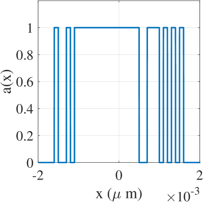
4.3. Design of aperture codes
We now design an aperture code that is capable of resolving both space and spectrum at high-resolutions. Our use of coded apertures is inspired by seminal works in coded photography for motion and defocus deblurring [Raskar et al., 2006; Veeraraghavan et al., 2007; Levin et al., 2007].
Observation.
Recall that the rainbow plane image is a convolution between a 1D spectral profile and a 2D aperture code . This convolution is one dimensional, i.e., along the -axis; hence, we can significantly simplify the code design problem by choosing an aperture of the form
| (8) |
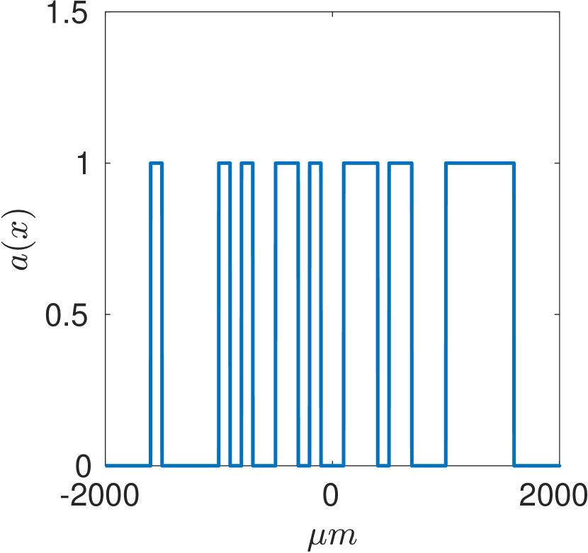
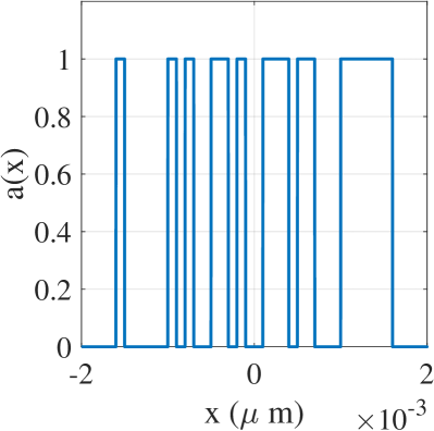
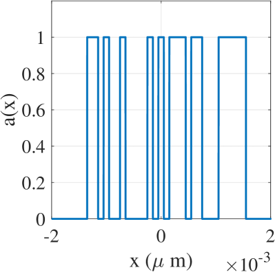
with being as large as possible. The choice of the rect function along the -axis leads to a high light throughput as well as a compact spatial blur along the -axis. For ease of fabrication, we further restrict the aperture code to be binary and of the form
| (9) |
where when and zero otherwise. Hence, the mask design reduces to finding an -bit codeword . The term , with units in length, specifies the physical dimension of each bit in the code. We fix its value based on the desired spectral resolution. For example, for mm and grooves/mm, a desired spectral resolution of nm would require m.
Our goal is to design masks that enable the following:
-
•
High light throughput. For a given code length , we seek codes with large light throughput which is equal to the number of ones in the code word
-
•
Invertibility of the spatial and spectral blur. The code is designed such that the resulting spatial and spectral blur are both invertible.
An invertible blur can be achieved by engineering its PSD to be flat. Given that the spectrum is linearly convolved with , a -point DFT of the code word captures all the relevant components of the PSD of . Denoting this -point DFT of as , we aim to maximize its minimum value in magnitude. Recall from (7) that the spatial PSF is the power spectral density (PSD) of , with suitable scaling. Specifically, the Fourier transform of spatial blur is given by , where is the linear autocorrelation of and represents spatial frequencies. From (9), we get,
| (10) |
where is the discrete linear autocorrelation of . Thus, it is sufficient to maximize to obtain an invertible spatial blur.
We select an aperture code that leads to invertible blurs for both space and spectrum by solving the following optimization problem:
| (11) |
under the constraint that the elements of are binary-valued, and is a constant. For code length sufficiently small, we can simply solve for the optimal code via exhaustive search of all code words. We used and an exhaustive search for the optimal code took over a day. The resulting code and its performance is shown in Figure 21 and 7; we used m and mm for this result. A brute force optimization is not scalable for larger codes. Instead of searching for optimal codes, we can search for approximately optimal codes by iterating over a few candidate solutions. This strategy has previously been explored in [Raskar et al., 2006], where 6 million candidate solutions are searched for a 52-dimensional code.
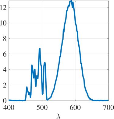
Figure 7 shows the frequency response of both spectral and spatial blurs for the 32-dimensional optimized code. The advantages of optimized codes are immediately evident — an open aperture has several nulls in spectral domain, while a slit attenuates all high spatial frequencies. The optimized code retains all frequencies in both domains, while increasing light throughput.
5. Synthetic experiments
()


,
PSNR: dB

,
PSNR: dB

,
PSNR: dB

,
PSNR: dB

,
PSNR: dB

,
PSNR: dB
()


,
PSNR: dB

,
PSNR: dB

,
PSNR: dB

,
PSNR: dB

,
PSNR: dB

,
PSNR: dB
We tested KRISM via simulations on three different datasets, listed in Table 2, and compared against existing approaches. For all methods, we simulated both photon and readout noise respectively as Poisson and Gaussian random variables. All KRISM simulations were done with diffraction effects due to coded aperture.
We quantify performance through compression in measurements which is ratio of number of unknowns to measurements and peak signal to noise ratio (PSNR). Given a HSI matrix and its reconstruction , we define peak SNR as
where RMSE is the root mean squared error defined as
| (12) |
![[Uncaptioned image]](/html/1801.09343/assets/x13.png)
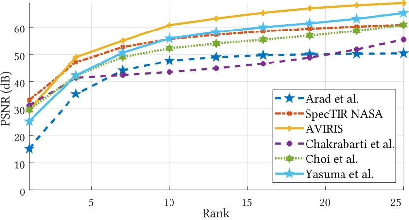
Comparison with snapshot techniques.
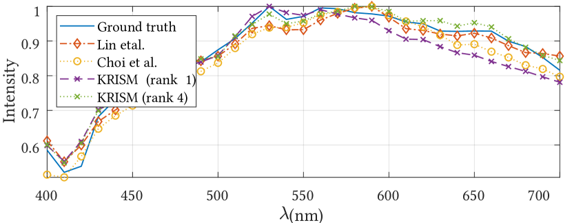
Snapshot techniques such as CASSI [Wagadarikar et al., 2008] and spatial-spectral encoded CS [Lin et al., 2014a] recover HSI from a single image and hence are appropriate for video-rate hyperspectral imaging. In contrast, KRISM is not a snapshot technique since, at the very least it requires the measurement of an image and a spectral profile. Nevertheless, we compare KRISM against snapshot techniques by varying the number of KRISM iterations. Figure 9 shows performance of these methods with varying number of measurements on KAIST and Harvard datasets. We observe that in the setting closest to snapshot mode, Choi et al. [2017] and Lin et al. [2014a] do outperform KRISM; this is to be expected since after a single iteration, KRISM provides only a rank-1 approximation. As the number of KRISM iterations are increased (which allows approximations of higher ranks), KRISM performance improves. KRISM enjoys advantages when we look at computational cost for reconstruction. The reconstruction time for Choi et al. [2017] is more than 10 minutes111We used code, dataset and model from https://github.com/KAIST-VCLAB/deepcassi even with multiple GPUs, while it runs to several hours for Lin et al. [2014a]222We used code, dataset and overcomplete dictionary from the paper itself.. In contrast, KRISM requires practically no reconstruction time for recovering the HSI as we directly measure the singular vectors.
()


PSNR: dB

PSNR: dB

,
PSNR: dB

,
PSNR: dB
Comparison with multi-frame techniques.
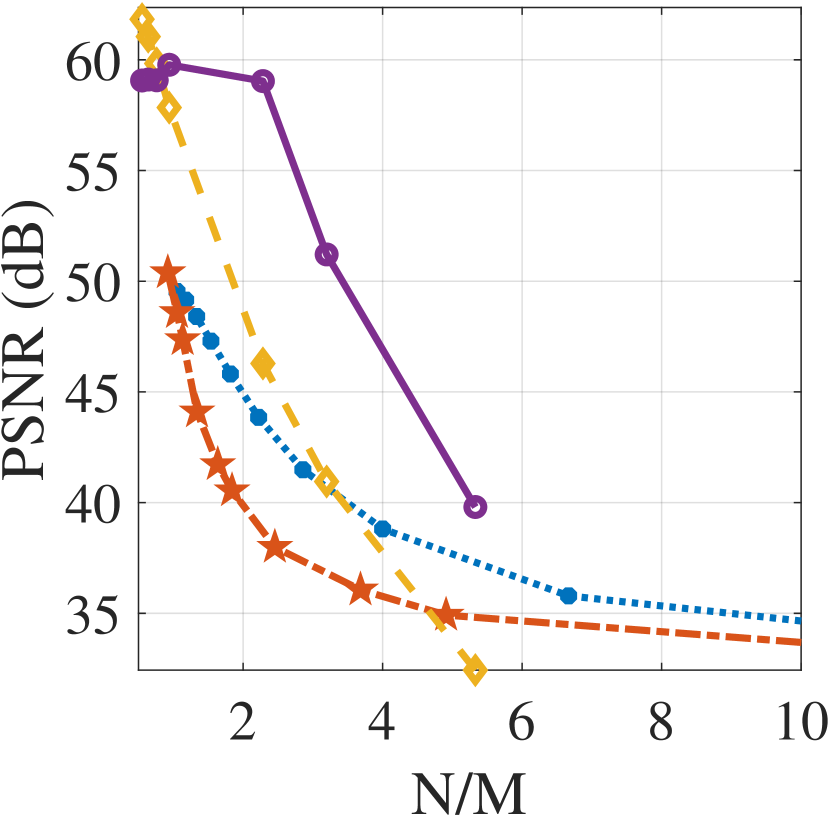
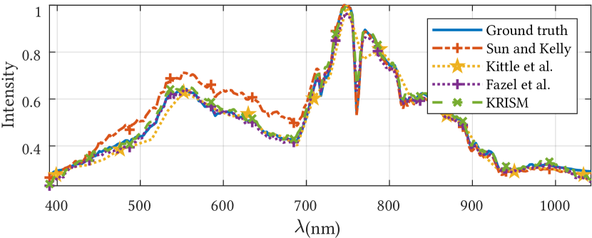
Since KRISM is essentially a multi-frame technique, we compare against multi-frame version of CASSI [Kittle et al., 2010], and spatially-multiplexed hyperspectral imager [Sun and Kelly, 2009]. We simulate spatially-multiplexed HSI imager via randomly permuted Hadamard multiplexed spectra and recover using sparsity of individual bands in wavelet domain. Note that the compression ratio is lower for Kittle et al. [2010] and Sun and Kelly [2009] since the results were inaccurate for higher compressions333Please see supplementary for further details.. Figure 10 shows a comparison of recovered spatial and spectral images for ICVL dataset. The poor performance of Kittle et al. [2010] is due to usage of a translational mask to get multiple measurements. On the other hand, Sun and Kelly [2009] performs poorly as multiplexing is done only in the spatial domain. Performance can be improved if we multiplex in the spectral domain as well; the resulting method is the low-rank CS approach proposed by Fazel et al. [2008]. This results in an increase in accuracy with fewer measurements, as seen in Figure 10 (f). Note that CS-based techniques are based on random projections and are not adapted to the scene. In contrast, KRISM adaptively computes a low-rank approximation leading to an increase in accuracy with the same number of measurements as Fazel et al. [2008].
Based on these simulations, we conclude that KRISM is indeed a compelling methodology when spatial and spectral resolution are high — a desirable operating point in many applications. When the number of spectral bands are smaller, the gains are modest, but nevertheless present. In the next section, we provide an optical schematic for implementing KRISM.
6. The KRISM Optical setup
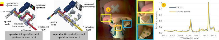
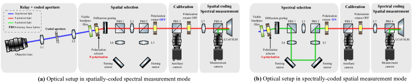
We now present an optical design for implementing the two operators presented in Section 3 and analyzed in Section 4. For efficiencies in implementation, we propose a novel design that combines both operators into one compact setup. Figure 11 shows a schematic that uses polarization to achieve both operators with a single SLM and a single camera. First, in Figure 11(a), an SLM is placed 2 away from the grating, and an image sensor 2 away from the SLM, implementing spectrally coded spatial measurement operator . In Figure 11(b), light follows an alternate path where in the SLM is 4 away from the grating; the camera is still 2 away from the SLM. This light path allows us to achieve the spatial-coded spectral measurement operator . The two light pathways are combined using a combination of polarizing beam splitters (PBS) and liquid crystal rotators (LC). The input light is pre-polarized to be either S-polarized or P-polarized. When the light is P-polarized, the SLM is effectively 2 units away from the grating leading to implementation of , the spectrally-coded imager. When the light is S-polarized, the SLM is 4 units away, provided the polarizing beamsplitter, PBS 3 was absent. To counter this, an LC rotator is placed before PBS 3 that rotates S-polarization to P-polarization when switched on. Hence, when S-light is input in conjugation with the rotator being switched on, we achieve the operator , a spatially-coded spectrometer. By simultaneously controlling the polarization of input light and the LC rotator, we can implement both and operators with a single camera and SLM pair.
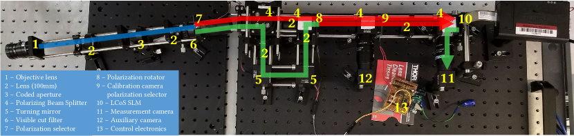
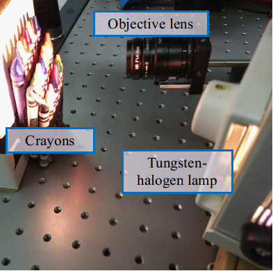
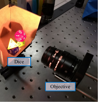
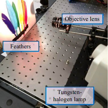
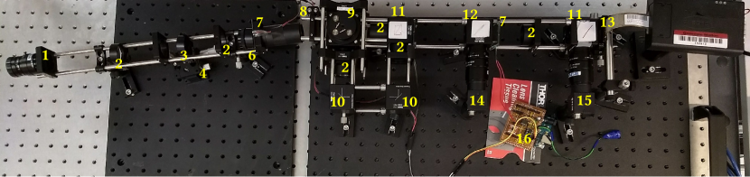
Figure 12 shows our lab prototype with the entire light pathway including the coded aperture placed in the relay system between the objective lens and diffraction grating. The input polarization is controlled by using a second LC rotator with a polarizer, placed before the diffraction grating. Finally, an auxiliary camera is used to image the pattern displayed on the SLM. This camera is used purely for alignment of the pattern displayed on the SLM. A detailed list of components can be found in the supplemental material.
Calibration.
Our optical setup requires three calibration processes. The first one is camera to SLM calibration. We used an auxiliary camera (Component 12 in Figure 12) that is directly focused on the SLM for this purpose. The second one is calibration of wavelengths. We used several narrowband filters to identify the location of wavelengths. Finally, the third one is radiometric calibration. We used a calibrated Tungsten-Halogen light source to estimate the spectral response of the setup. A detailed description of the calibration procedure can be found in the supplementary material.
System characterization.
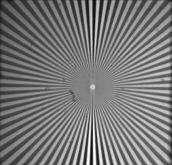
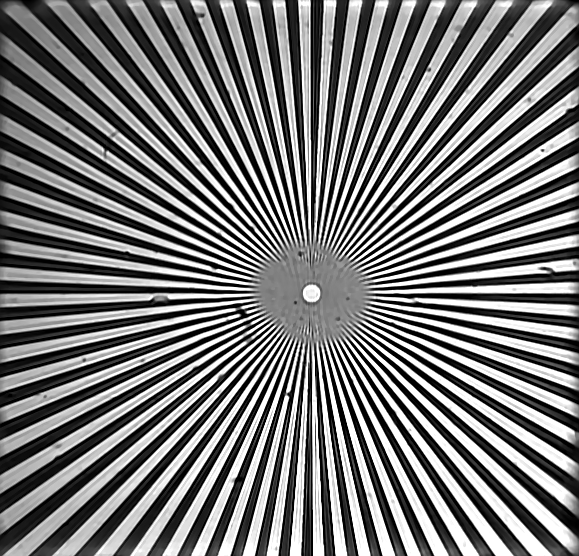
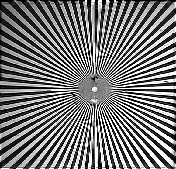
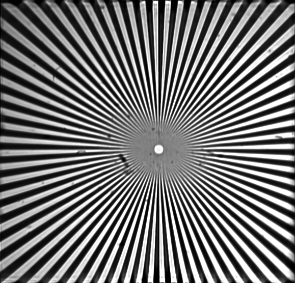
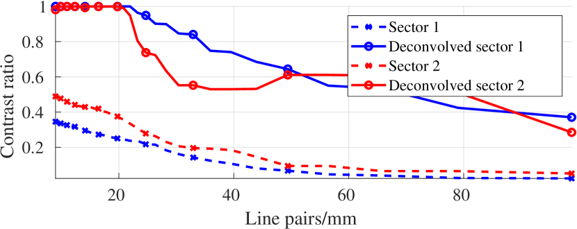
Spectral resolution (FWHM) of the setup was computed using several 1nm narrowband filters across visible wavelengths. Our optical setup provided an FWHM of 2.9nm. Spatial resolution was computed by capturing photo of a Siemens star, and then deconvolving with a point-spread function obtained by capturing image of a pinhole. The frequency that achieved 30% of the modulation transfer function, MTF30, was found to be nearly 0.4 line pairs/pixel. All computation details, as well as relevant figures, can be found in the supplementary material.
Diffraction due to LCoS pattern.
Since the SLM is placed away from spectral or spatial measurements, the displayed pattern introduces diffraction blur, creating a non-linear measurement system. To counter this, we add a constant offset to both positive and negative patterns, which makes the diffraction blur compact enough that the non-linearities can be neglected.
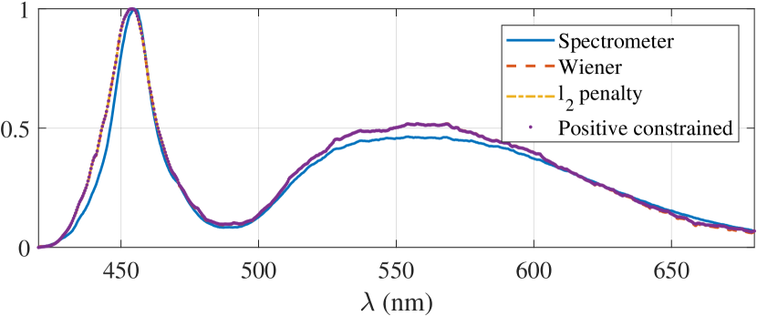
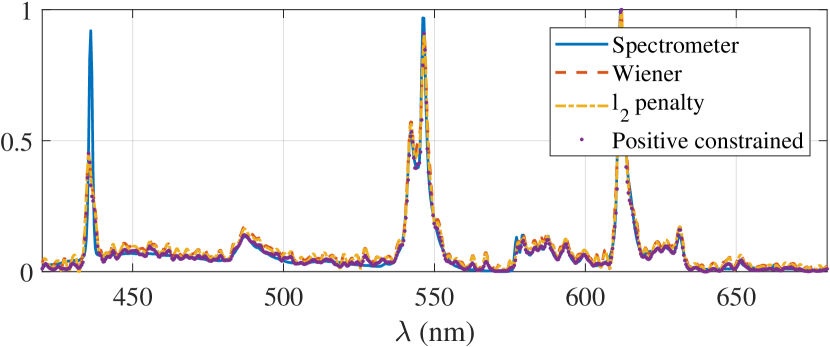
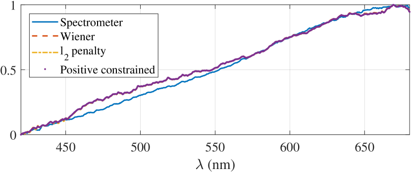
Spectral deconvolution.
Measurements by our optical system return spectra at each point, convolved by the aperture code. To get the true spectrum, we deconvolved the measured singular vector using a smoothness prior. The specific objective function we used:
| (13) |
where is the true spectrum, is the measured spectrum, is the aperture code, is the first order difference of , and is weight of penalty term. Solution to (13) was computed using conjugate gradient descent. Higher favors smoother spectra, and hence is preferred for illuminants with smooth spectra, such as tungsten-halogen bulb or white LED. For peaky spectra such as CFL, a lower value of is preferred. In our experiments, we found to be appropriate for peaky spectra, whereas, was appropriate for experiments with tungsten-halogen illumination. We compare performance of various deconvolution algorithms in the supplementary section.
Spatial deconvolution.
Equation (7) suggests that the spatial blur kernel varies across different spectral bands. More specifically, the blur kernels at two different spectra are scaled versions of each other. However, we observed that the variations in blur kernels were not significant when we image over a small waveband — for example, the visible waveband of nm. Given this, we approximate the spatial blur as being spectrally independent, which leads to the following expression:
| (14) |
where is the spatial blur. We estimated the spatial blur kernel by imaging a pinhole and subsequently deconvolved the spatial singular vectors. We used a TV prior based deconvolution using the technique in [Bioucas-Dias and Figueiredo, 2007] using the image of a pinhole as the PSF. Details of the deconvolution procedure are in the supplementary section.
7. Real Experiments
We present several results from real experiments which show the effectiveness of KRISM. We evaluate the ability to measure singular vectors with high accuracy, and high spatial and spectral resolution capabilities. Unless specified, experiments involved a capture of a rank-4 approximation of the HSI, with 6 spectral and 6 spatial measurements. Lanczos iterations were initialized with all-ones spatial image to speed up convergence. HSIs were acquired with a spatial resolution of pixels and a spectral resolution of bands between 400nm to 700nm, with 3 nm FWHM. For verifying spectroradiometric capabilities, we obtained spectral measurements at a small set of spatial points using an Ocean Optics FLAME spectrometer. We use spectral angular mapper (SAM) [Yuhas et al., 1992] similarity and PSNR between spectra measured by our optical setup and that measured with a spectrometer. SAM between two vectors and is defined as .
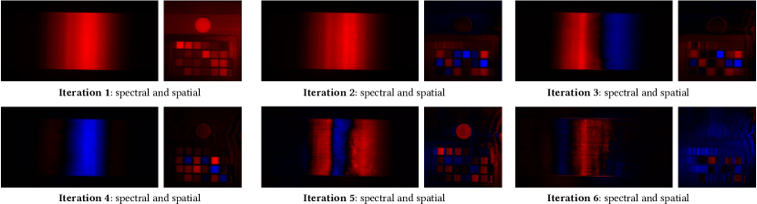
Visualization of Lanczos iterations
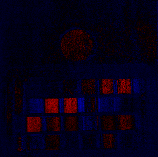
Figure 13 shows iterations for the “Color checker” scene in Figure 17. The algorithm initially captures brightest parts of the image, corresponding to the spectralon, and the white and yellow patches. Consequently, by iteration 5, the blue and red parts of the image are isolated. The iterations are representative of the signal energy in various wavelengths. Maximum energy is concentrated in yellow wavelengths, due to tungsten-halogen illuminant and spectral response of the camera. This is then followed by the red wavelengths, and finally the blue wavelengths.
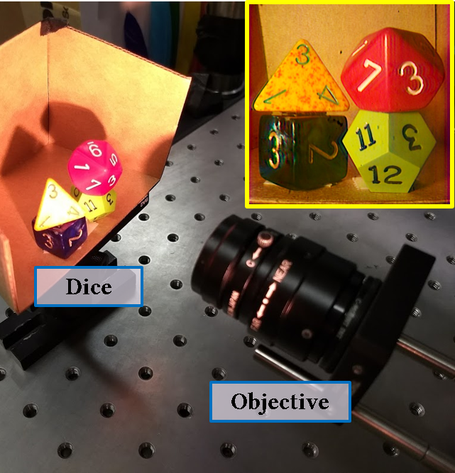
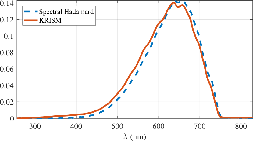
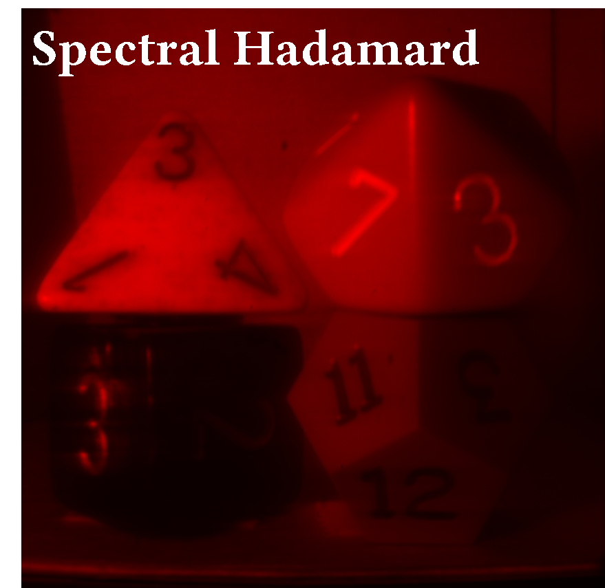
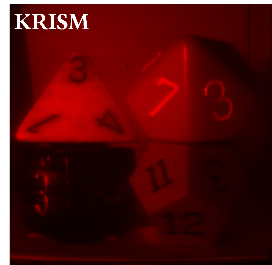
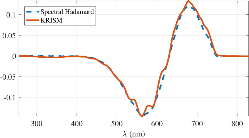
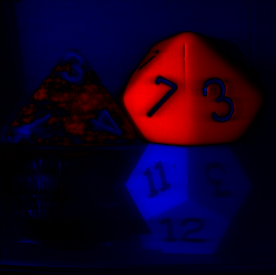
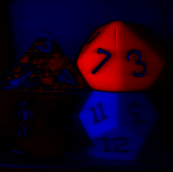
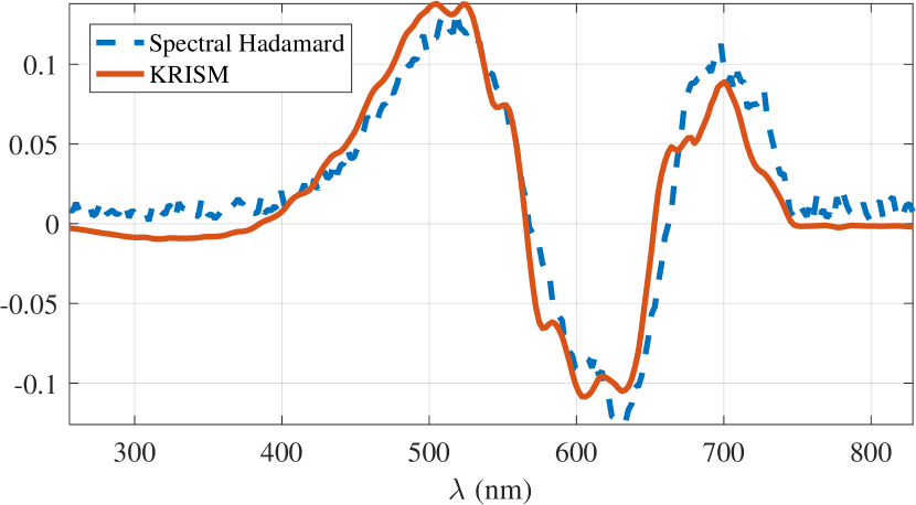
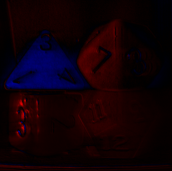
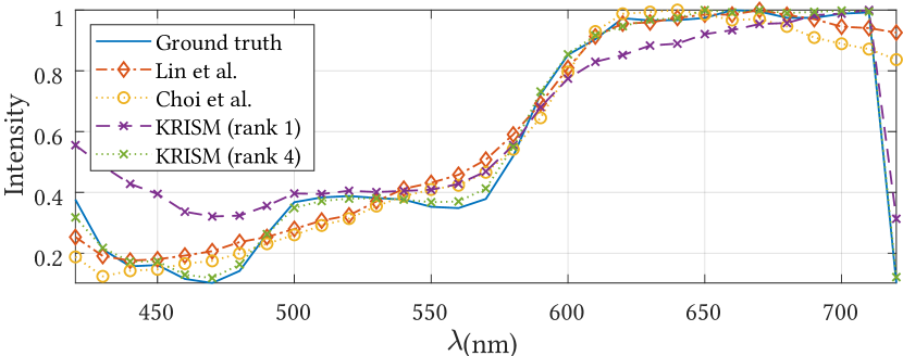
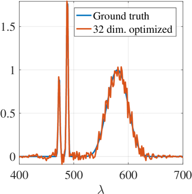
Comparison of measured singular vectors.
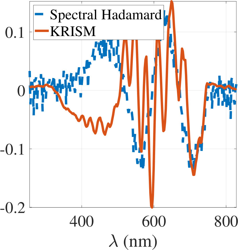
We obtain the complete hyperspectral image through a permuted Hadamard multiplexed sampling in the spectral domain for comparison with ground-truth singular vectors. We chose a scene with four colored dice for this purpose, shown in Figure 14 (a). We then computed 4 singular vectors of spectrally Hadamard-multiplexed data. Figure 14 shows a comparison of the spatial and spectral singular vectors. The singular vectors obtained via Krylov subspace technique are close to the ones obtained through Hadamard sampling. On an average, the reconstruction accuracy between KRISM and Hadamard multiplexing was found to be greater than 30dB, while the angle between the singular vectors was no worse than , with the top three singular vector having an error smaller than . Hadamard sampling took 49 minutes while KRISM took under 2 minutes for 6 spatial and 6 spectral measurements, thus offering a speedup of .
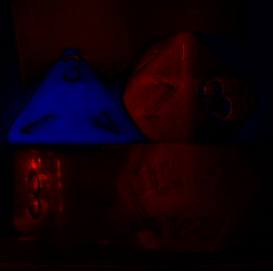
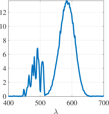
Peaky spectrum illumination
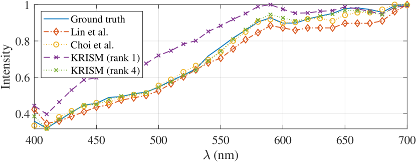
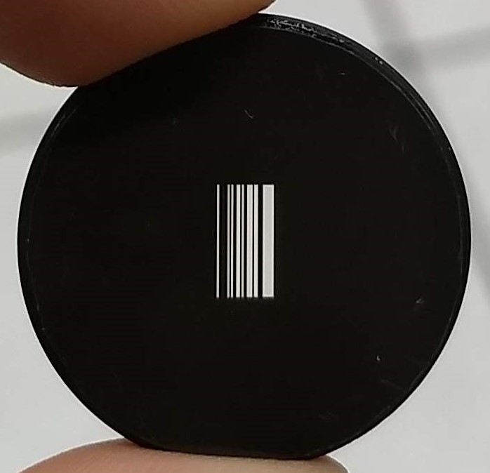
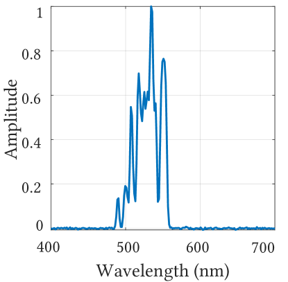
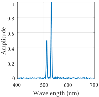
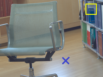
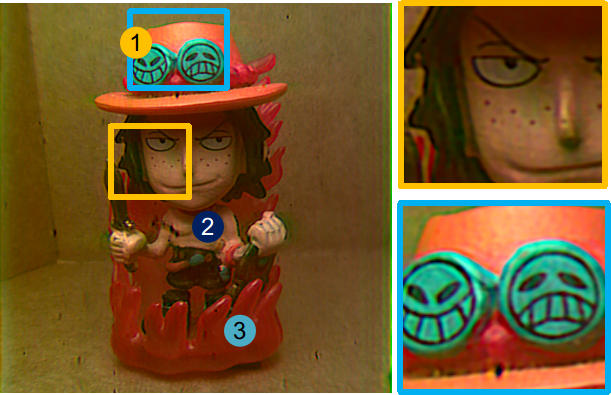
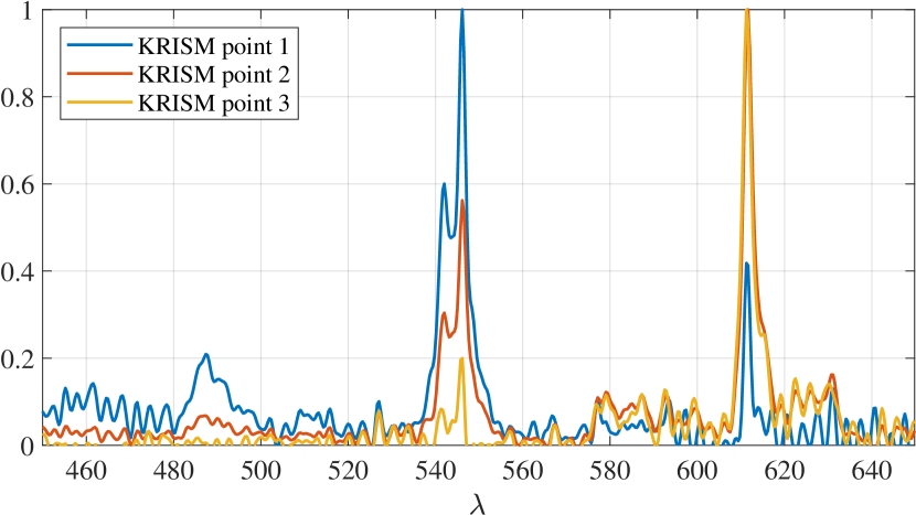
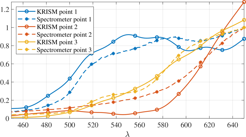
We imaged a small toy figurine of “Chopper”, placed under CFL, which has a peaky spectrum, to test high spatio-spectral resolving capability. Figure 1 shows the rendered RGB image and spectra at a representative location. Spectra at a selected spatial point, as measured by KRISM, and a spectrometer are shown as well. The SAM between spectrum measured by KRISM and that measured by spectrometer was found to be . Notice that the location of the peaks, as well as the heights match accurately. Indeed, the chopper example establishes the high spatio-spectral resolution capabilities of KRISM.
Diverse real experiments.
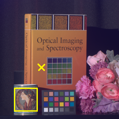
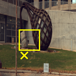
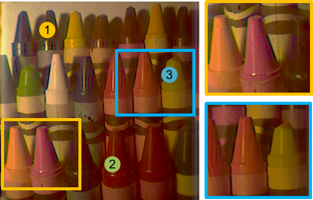
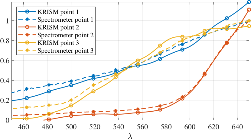
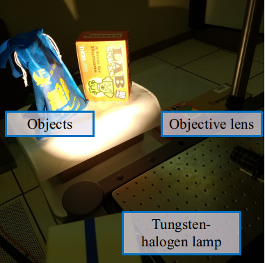
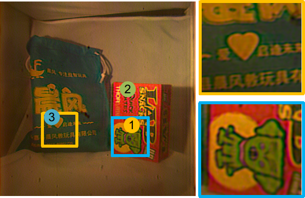
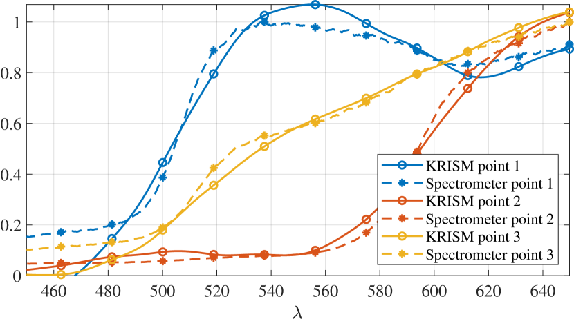
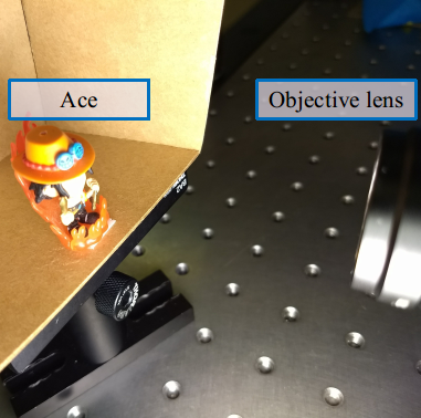
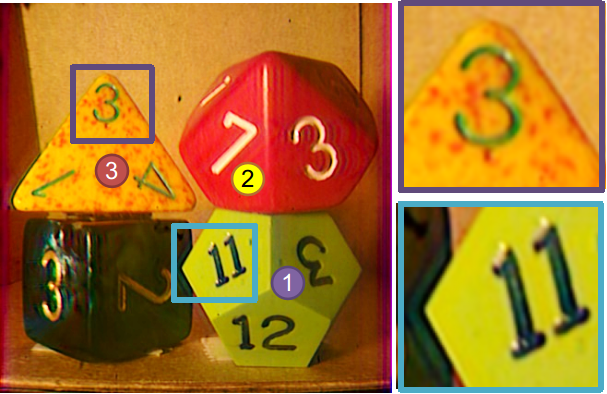
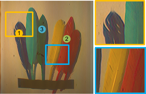
Figure 16 shows several real world examples captured with our optical setup, with a diverse set of objects. For verification with ground truth, we captured spectral profiles at select spatial locations. The “Dice” and “Objects” scene captures several more colorful objects with high texture. The zoomed-in pictures show the spatial resolution, while the comparison of spectra highlights the fidelity of our system as a spectral measurement tool. “Ace” scene was captured by placing the toy figurine under CFL illuminant, which is peaky. We could not obtain ground truth with a spectrometer, as the toy was too small to reliably probe with a spectrometer. The peaks are located within 2nm of ground truth peaks, and the relative heights of the peaks match the underlying color. “Crayons” scene consists of numerous colorful wax crayons illuminated with a tungsten-halogen lamp. The closeness of spectra with respect to spectrometer readings shows the spectral performance of our setup. Finally, “Feathers” consists of several colorful feathers illuminated by tungsten-halogen lamp. The fine structure of feathers is well captured by our setup.


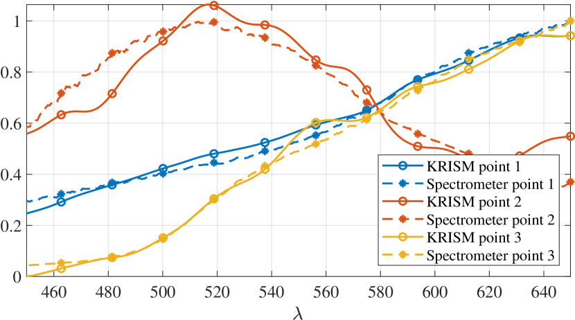
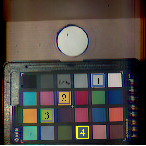
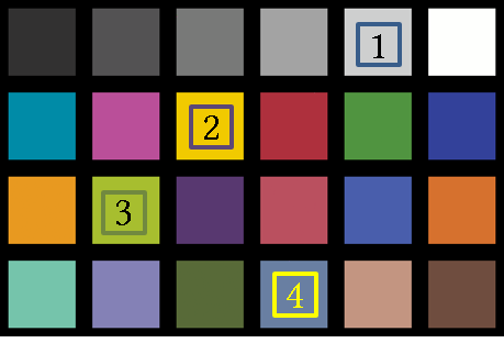
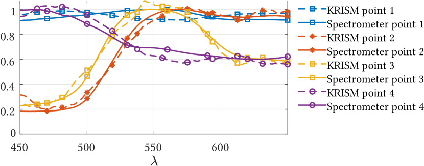
Color checker.
Since our setup is optimized for viewing in 400nm-700nm, we evaluated our system on the 24-color Macbeth color chart. The Macbeth color chart consists of a wide gamut of colors in visible spectrum that are spectrally well separated, and forms a good test bench for visible spectrometry. We placed the “Color passport” and spectralon plug in front of our camera and illuminated it with a tungsten-halogen DC light source. The spectralon has a spectrally flat response, and hence helps estimate the spectral response of the illuminant+spectrometer system. This enables measurement of true radiance of the color swatches. Since the spectra is smooth, we used least squares recovery of the spectrum, with penalty on the first difference of spectral singular vectors. The captured data was then normalized by dividing spectrum of all points with the spectrum of the spectralon. Figure 17 shows the captured image against reference color chart along with spectra at select locations plotted along with ground truth spectra. On an average, the PSNR between spectra measured by KRISM and that measured by spectrometer is greater than 25dB, while the SAM is less than .
8. Discussion and conclusion
We presented a novel hyperspectral imaging methodology called KRSIM, and provided an associated novel optical system for enabling optical computation of hyperspectral scenes to acquire the top few singular vectors in a fast and efficient manner. Through several real experiments, we establish the strength of KRISM in three important aspects: 1) the ability to capture singular vectors of the hyperspectral image with high fidelity, 2) the ability to capture an approximation of the hyperspectral image with or faster acquisition rate compared to Nyquist sampling, and 3) the ability to measure simultaneously at high spatial and spectral resolution. We believe that our setup will trigger several new experiments in adaptive imaging for fast and high resolution hyperspectral imaging.
Added advantages.
There are two additional advantages to KRISM. One, since we capture the top few singular vectors directly, there is a data compression from the acquisition itself. Two, the only recovery time involves deconvolution of a few spatial and spectral singular vectors, which is significantly less than the time required for recovery of hyperspectral images from CS measurements.
Beyond low-rank volumes.
Key to our paper is the assumption that the underlying HSI is low-rank. Sensing a high rank HSI will require several measurements which negates the benefits of KRISM. However, there are several other matrix sampling techniques that rely on row or column sensing [Hašan et al., 2007; Ou and Pellacini, 2011] to capture information about high rank matrices in an efficient manner. Since the proposed setup is capable of computing arbitrary matrix-vector products, such matrix sampling techniques can be implemented efficiently.
Effect of photon noise
Although Krylov subspace based methods are very robust to noise [Simoncini and Szyld, 2003], the quality of the singular vectors degrade as the rank of acquisition is increased (see Figure 18). This is primarily due to photon noise, as we progressively block most of the energy contained in initial singular vectors. This can be mitigated by increasing the exposure time of measurements for higher singular vectors. All said, the problem of noisy higher singular vectors exists with any kind of sampling scheme and hence needs separate attention via a good noise model.
9. Acknowledgement
The authors thank Prof. Ioannis Gkioulekas (Robotics Institute, CMU) for valuable feedback, and Ms. Yi Hua (ECE Department, CMU) for help with making the figures. The authors acknowledge support via the NSF CAREER grant CCF-1652569, the National Geospatial-Intelligence Agency’s Academic Research Program (Award No. HM0476-17-1-2000), and the Intel ISRA on compressive sensing. Vishwanath Saragadam also gratefully acknowledges support via the Prabhu and Poonam Goel fellowship.
References
- [1]
- Arad and Ben-Shahar [2016] Boaz Arad and Ohad Ben-Shahar. 2016. Sparse recovery of hyperspectral signal from natural RGB images. In European Conf. Comp. Vision (ECCV).
- Arce et al. [2014] Gonzalo R Arce, David J Brady, Lawrence Carin, Henry Arguello, and David S Kittle. 2014. Compressive coded aperture spectral imaging: An introduction. IEEE Signal Processing Magazine 31, 1 (2014), 105–115.
- Arguello and Arce [2013] Henry Arguello and Gonzalo R Arce. 2013. Rank minimization code aperture design for spectrally selective compressive imaging. IEEE Trans. Image Processing 22, 3 (2013), 941–954.
- Athale and Collins [1982] Ravindra A Athale and William C Collins. 1982. Optical matrix–matrix multiplier based on outer product decomposition. Appl. Optics 21, 12 (1982), 2089–2090.
- Baek et al. [2017] Seung-Hwan Baek, Incheol Kim, Diego Gutierrez, and Min H Kim. 2017. Compact single-shot hyperspectral imaging using a prism. ACM Trans. Graphics 36, 6 (2017), 217:1–12.
- Baraniuk [2007] Richard G Baraniuk. 2007. Compressive sensing. IEEE Signal Processing Magazine 24, 4 (2007), 118–121.
- Bioucas-Dias and Figueiredo [2007] José M Bioucas-Dias and Mário AT Figueiredo. 2007. A new TwIST: Two-step iterative shrinkage/thresholding algorithms for image restoration. IEEE Trans. Image processing 16, 12 (2007), 2992–3004.
- Cao et al. [2016] Xun Cao, Tao Yue, Xing Lin, Stephen Lin, Xin Yuan, Qionghai Dai, Lawrence Carin, and David J Brady. 2016. Computational snapshot multispectral cameras: Toward dynamic capture of the spectral world. IEEE Signal Processing Magazine 33, 5 (2016), 95–108.
- Chakrabarti and Zickler [2011] Ayan Chakrabarti and Tod Zickler. 2011. Statistics of real-world hyperspectral images. In Comp. Vision and Pattern Recognition (CVPR).
- Choi et al. [2017] Inchang Choi, Daniel S. Jeon, Giljoo Nam, Diego Gutierrez, and Min H. Kim. 2017. High-quality hyperspectral reconstruction using a spectral prior. ACM Trans. Graphics 36, 6 (2017), 218:1–13.
- Cloutis [1996] Edward A Cloutis. 1996. Review Article Hyperspectral geological remote sensing: Evaluation of analytical techniques. Intl. J. Remote Sensing 17, 12 (1996), 2215–2242.
- Fazel et al. [2008] Maryam Fazel, Emmanuel J Candes, Benjamin Recht, and Pablo A Parrilo. 2008. Compressed sensing and robust recovery of low rank matrices. In Asilomar Conf. Signals, Systems and Comp.
- Finlayson et al. [1994] Graham D Finlayson, Mark S Drew, and Brian V Funt. 1994. Color constancy: Generalized diagonal transforms suffice. J. Optical Society of America A 11, 11 (1994), 3011–3019.
- Ge et al. [2006] Hongya Ge, Ivars P Kirsteins, and Louis L Scharf. 2006. Data dimension reduction using Krylov subspaces: Making adaptive beamformers robust to model order-determination. In Intl. Conf. Acoustics Speech and Signal Processing (ICASSP).
- Ge et al. [2004] Hongya Ge, LL Scharf, and Magnus Lundberg. 2004. Reduced-rank multiuser detectors based on vector and matrix conjugate gradient Wiener filters. In Workshop on Signal Processing Adv. Wireless Communications.
- Gehm et al. [2007] Michael E Gehm, Renu John, David J Brady, Rebecca M Willett, and Timothy J Schulz. 2007. Single-shot compressive spectral imaging with a dual-disperser architecture. Optics Express 15, 21 (2007), 14013–14027.
- Golbabaee and Vandergheynst [2012] Mohammad Golbabaee and Pierre Vandergheynst. 2012. Hyperspectral image compressed sensing via low-rank and joint-sparse matrix recovery. In Intl. Conf. Acoustics, Speech and Signal Processing (ICASSP).
- Golub and Kahan [1965] Gene Golub and William Kahan. 1965. Calculating the singular values and pseudo-inverse of a matrix. J. Society for Industrial and Appl. Mathematics, Series B: Numerical Analysis 2, 2 (1965), 205–224.
- Goodman [2005] Joseph W Goodman. 2005. Introduction to Fourier optics. Roberts and Company Publishers.
- Harsanyi and Chang [1994] Joseph C Harsanyi and C-I Chang. 1994. Hyperspectral image classification and dimensionality reduction: An orthogonal subspace projection approach. IEEE Trans. Geoscience and Remote Sensing 32, 4 (1994), 779–785.
- Harwit and Sloane [1979] Martin Harwit and Neil J Sloane. 1979. Hadamard Transform Optics.
- Hašan et al. [2007] Miloš Hašan, Fabio Pellacini, and Kavita Bala. 2007. Matrix row-column sampling for the many-light problem. ACM Trans. Graphics 26, 3 (2007), 26:1–10.
- Hernandez et al. [2007] Vicente Hernandez, Jose E Roman, Andres Tomas, and Vicente Vidal. 2007. Restarted Lanczos bidiagonalization for the SVD in SLEPc. Technical Report.
- Hui et al. [2018] Zhuo Hui, Kalyan Sunkavalli, Sunil Hadap, and Aswin C. Sankaranarayanan. 2018. Illuminant spectra-based source separation using flash photography. In Comp. Vision and Pattern Recognition (CVPR).
- Jeon et al. [2016] Daniel S Jeon, Inchang Choi, and Min H Kim. 2016. Multisampling compressive video spectroscopy. In Comp. Graphics Forum.
- Kauvar et al. [2015] Isaac Kauvar, Samuel J Yang, Liang Shi, Ian McDowall, and Gordon Wetzstein. 2015. Adaptive color display via perceptually-driven factored spectral projection. ACM Trans. Graphics 34, 6 (2015), 165:1–10.
- Kim et al. [2012] Min H Kim, Todd Alan Harvey, David S Kittle, Holly Rushmeier, Julie Dorsey, Richard O Prum, and David J Brady. 2012. 3D imaging spectroscopy for measuring hyperspectral patterns on solid objects. ACM Trans. Graphics 31, 4 (2012), 38:1–11.
- Kittle et al. [2010] David Kittle, Kerkil Choi, Ashwin Wagadarikar, and David J Brady. 2010. Multiframe image estimation for coded aperture snapshot spectral imagers. Appl. Optics 49, 36 (2010), 6824–6833.
- Lee et al. [2000] Te-Won Lee, Thomas Wachtler, and Terrence J Sejnowski. 2000. The spectral independent components of natural scenes. In Intl. Workshop on Biologically Motivated Comp. Vision.
- Levin et al. [2007] Anat Levin, Rob Fergus, Frédo Durand, and William T Freeman. 2007. Image and depth from a conventional camera with a coded aperture. ACM Trans. Graphics 26, 3 (2007), 70:1–10.
- Li et al. [2012] Chengbo Li, Ting Sun, Kevin F Kelly, and Yin Zhang. 2012. A compressive sensing and unmixing scheme for hyperspectral data processing. IEEE Trans. Image Processing 21, 3 (2012), 1200–1210.
- Lin et al. [2014a] Xing Lin, Yebin Liu, Jiamin Wu, and Qionghai Dai. 2014a. Spatial-spectral encoded compressive hyperspectral imaging. ACM Trans. Graphics 33, 6 (2014), 233:1–11.
- Lin et al. [2014b] Xing Lin, Gordon Wetzstein, Yebin Liu, and Qionghai Dai. 2014b. Dual-coded compressive hyperspectral imaging. Optics Letters 39, 7 (2014), 2044–2047.
- Mohan et al. [2008] Ankit Mohan, Ramesh Raskar, and Jack Tumblin. 2008. Agile spectrum imaging: Programmable wavelength modulation for cameras and projectors. In Comp. Graphics Forum.
- O’Toole and Kutulakos [2010] Matthew O’Toole and Kiriakos N Kutulakos. 2010. Optical computing for fast light transport analysis. ACM Trans. Graphics 29, 6 (2010), 164:1–12.
- Ou and Pellacini [2011] Jiawei Ou and Fabio Pellacini. 2011. LightSlice: Matrix slice sampling for the many-lights problem. ACM Trans. Graphics 30, 6 (2011), 179:1–8.
- Pan et al. [2003] Zhihong Pan, Glenn Healey, Manish Prasad, and Bruce Tromberg. 2003. Face recognition in hyperspectral images. IEEE Trans. Pattern Analysis and Machine Intelligence 25, 12 (2003), 1552–1560.
- Parkkinen et al. [1989] Jussi PS Parkkinen, J Hallikainen, and T Jaaskelainen. 1989. Characteristic spectra of Munsell colors. J. Optical Society of America A 6, 2 (1989), 318–322.
- Rajbenbach et al. [1987] Henri Rajbenbach, Yeshayahu Fainman, and Sing H Lee. 1987. Optical implementation of an iterative algorithm for matrix inversion. Appl. Optics 26, 6 (1987), 1024–1031.
- Raskar et al. [2006] Ramesh Raskar, Amit Agrawal, and Jack Tumblin. 2006. Coded exposure photography: Motion deblurring using fluttered shutter. ACM Trans. Graphics 25, 3 (2006), 795–804.
- Rasti et al. [2013] Behnood Rasti, Johannes R Sveinsson, Magnus O Ulfarsson, and Jon Atli Benediktsson. 2013. Hyperspectral image denoising using a new linear model and sparse regularization. In IEEE Intl. Geoscience and Remote Sensing Symposium.
- Rueda et al. [2016] Hoover Rueda, Henry Arguello, and Gonzalo R Arce. 2016. Compressive spectral testbed imaging system based on thin-film color-patterned filter arrays. Appl. Optics 55, 33 (2016), 9584–9593.
- Rueda et al. [2017] Hoover Rueda, Henry Arguello, and Gonzalo R Arce. 2017. High-dimensional optimization of color coded apertures for compressive spectral cameras. In European Signal Processing Conf.
- Saragadam et al. [2017] Vishwanath Saragadam, Jian Wang, Xin Li, and Aswin Sankaranarayanan. 2017. Compressive spectral anomaly detection. In Intl. Conf. Comp. Photography (ICCP).
- Simoncini and Szyld [2003] Valeria Simoncini and Daniel B Szyld. 2003. Theory of inexact Krylov subspace methods and applications to scientific computing. SIAM J. Scientific Comp. 25, 2 (2003), 454–477.
- SpecTIR [2019] SpecTIR. 2019. SpecTIR, Advanced hyperspectral and geospatial Solutions. http://www.spectir.com/free-data-samples/. (2019). [Online; accessed: 2019-07-01].
- Sun and Kelly [2009] Ting Sun and Kevin Kelly. 2009. Compressive sensing hyperspectral imager. In Comp. Optical Sensing and Imaging.
- Takatani et al. [2017] Tsuyoshi Takatani, Takahito Aoto, and Yasuhiro Mukaigawa. 2017. One-shot hyperspectral imaging using faced reflectors. In Comp. Vision and Pattern Recognition (CVPR).
- Tarabalka et al. [2010] Yuliya Tarabalka, Jocelyn Chanussot, and Jon Atli Benediktsson. 2010. Segmentation and classification of hyperspectral images using watershed transformation. Pattern Recognition 43, 7 (2010), 2367–2379.
- Tian et al. [2005] Zhi Tian, Hongya Ge, and Louis L Scharf. 2005. Low-complexity multiuser detection and reduced-rank Wiener filters for ultra-wideband multiple access. In Intl. Conf. Acoustics, Speech, and Signal Processing (ICASSP).
- Veeraraghavan et al. [2007] Ashok Veeraraghavan, Ramesh Raskar, Amit Agrawal, Ankit Mohan, and Jack Tumblin. 2007. Dappled photography: Mask enhanced cameras for heterodyned light fields and coded aperture refocusing. ACM Trans. Graphics 26, 3 (2007), 69:1–12.
- Vijaya Kumar and Casasent [1981] Bhagavatula Vijaya Kumar and David Casasent. 1981. Eigenvector determination by iterative optical methods. Appl. Optics 20, 21 (1981), 3707–3710.
- Wagadarikar et al. [2008] Ashwin Wagadarikar, Renu John, Rebecca Willett, and David Brady. 2008. Single disperser design for coded aperture snapshot spectral imaging. Appl. Optics 47, 10 (2008), B44–B51.
- Waters et al. [2011] Andrew E Waters, Aswin C Sankaranarayanan, and Richard Baraniuk. 2011. SpaRCS: Recovering low-rank and sparse matrices from compressive measurements. In Adv. Neural Info. Processing Systems.
- Winter [1999] Michael E. Winter. 1999. N-FINDR: An algorithm for fast autonomous spectral end-member determination in hyperspectral data. In Proc. SPIE.
- Yasuma et al. [2010] Fumihito Yasuma, Tomoo Mitsunaga, Daisuke Iso, and Shree K Nayar. 2010. Generalized assorted pixel camera: Postcapture control of resolution, dynamic range, and spectrum. IEEE Trans. Image Processing 19, 9 (2010), 2241–2253.
- Yuhas et al. [1992] Roberta H Yuhas, Alexander FH Goetz, and Joe W Boardman. 1992. Discrimination among semi-arid landscape endmembers using the spectral angle mapper (SAM) algorithm. In Summaries of the Third Annual JPL Airborne Geoscience Workshop.
- Zhao and Yang [2015] Yong-Qiang Zhao and Jingxiang Yang. 2015. Hyperspectral image denoising via sparse representation and low-rank constraint. IEEE Trans. Geoscience and Remote Sensing 53, 1 (2015), 296–308.
Appendix A Supplementary Material
This article supplements the main paper with several simulations and real world experiments. The remainder of this article is organized as follows.
-
•
Section B — Derivation of spatio-spectral blur. We provide an in-depth derivation of the spatial and spectral blur relationship due to a coded aperture mentioned in Section 4 of the main paper.
-
•
Sections C — Code design. We provide details on the design of coded aperture, comparisons with alternate codes such as M-sequences, and specifications of the deconvolution technique used for both space and spectrum.
-
•
Section D — Details of optical implementation. We provide a comprehensive list of components used for building the setup.
-
•
Section E —Explanation of design choices. We discuss some of the design considerations for implementing our optical setup.
-
•
Section F — Calibration. This section serves as a guide for calibrating the proposed optical setup.
-
•
Section G — Real results. We provide additional visualization of the real data shown in the main paper.
-
•
Section H — Additional simulation results. We present some more simulations with emphasis on performance across a diverse set of datasets.
Appendix B Coded apertures for simultaneous sensing of space and spectrum

The main paper provided a brief derivation of the effect of coded aperture on spatial and spectral blur. We do a more rigorous proof here. Figure 19 explains the optical setup that we will consider for all our derivations. In particular, we place a coded aperture at plane P2, which introduces diffraction blur in both spatial and spectral measurements. We obtain spectral measurements on P4 and spatial measurements on P5. The goal of this section is to derive the relationship between measurements on P4 and P5 to the coded aperture and the scene’s HSI.
B.1. Assumptions
The first assumption is that the image is spatially incoherent, an assumption that is realistic for most real world settings. This implies that the spatial frequencies add up in intensities and not amplitudes. Next, the diffraction grating is assumed to disperse light along x-axis, which implies no dispersion along the y-axis. Finally, we assume an ideal thin lens model for all the lenses. This implies that the Fourier transform property of ideal thin lenses holds for all computations.
B.2. Basics
The derivation in the sequel relies on the so called Fourier transform property of lenses [Goodman, 2005]. Suppose that the complex-valued phase field at the plane is given as , where denote spatial coordinates on the plane and denotes the wavelength of light. Lets place an ideal thin lens with focal length at and whose optical axis is aligned along the axis. The Fourier transforming property states that the complex phasor field that is formed at the plane is given as
where is the 2D Fourier transform of along the first two dimensions.
We can compute the 2D Fourier transform of using the scaling property,
The negative signs in the argument of comes from the Fourier transform being the Hermitian of the inverse Fourier transform. If we now placed a second ideal thin lens of focal length at , then the field at can be computed as
The assembly above, with two lenses at and is referred to as a system. As we see above, the system replicates the field at at , barring a flip of the coordinate axis; this property is useful for the following discussion.
B.3. Propagation of signal
We will use Figure 19 as a guide for the derivation. An objective lens focuses a scene onto its image plane, denoted as P1. Assuming that all light is incoherent, let the complex phasor at P1 be denoted as ; note that intensity of this complex field is the hyperspectral image that we seek to measure, i.e.,
Since we assume an incoherent model, we analyze the system for a point light source and then extend it to a generic image by adding up only intensities.
Field at Plane P1.
Consider a point light source at with complex amplitude . The overall phasor field at P1 is given as
Field at Plane P2.
Using Fourier transform property of lens, we get the field on plane P2 to be,
| (15) |
where is the continuous 2D Fourier transform of along the first two dimensions. The field just after the coded aperture is given by,
| (16) |
Field at Plane P3.
Using Fourier transform property of lens a second time, the field just before the diffraction grating is
| (17) |
where is the continuous 2D FT of . Since the diffraction grating is assumed to disperse along x-axis, we model it as a series of infinite slits, given by,
| (18) |
where is the grove density of the diffraction grating, measured in grooves per unit length. The factor ensures that light does not get amplified as it propagates through the setup. The field just after the diffraction grating is hence given by,
| (19) |
Field at the Rainbow Plane P4.
To calculate the field at P4, we first need an expression for , the 2D Fourier transform of .
| (20) |
The field on plane P4 is given as:
| (21) |
where ”” represents continuous 2D convolution. Since we are only interested in the first order of diffraction, we set k = 1, giving us,
| (22) |
Field at the Spatial Plane P5.
Finally, the field on plane P5 is,
| (23) |
B.4. Measurement by camera
A camera can only measure intensity of the field. Assuming a camera with spectral response , the measurement on plane P4 is,
| (24) |
where is a 2D convolution and
Extending to a generic incoherent image case, we get the following expression,
| (25) |
where
We can observe from (25) that the image formed at the rainbow plane P4 is a convolution of the scene’s spectrum modified with the camera response as well as with the square of the aperture code.
Similarly, the intensity on plane P5 is given by,
| (26) |
where can be seen as the spatial PSF. Extending to a generic incoherent image case, we get the following expression,
| (27) |


(Spectrum PSNR: 31.9dB; Spatial PSNR: 27.2dB)


(Spectrum PSNR: 29.0dB; Spatial PSNR: 26.4dB)

(Spectrum PSNR: 29.4dB; Spatial PSNR: 26.4dB)
The expression above suggests that the image associated with each spectral channel is convolved with a different blur kernel; further, the blur kernel for different wavelengths are simple scaled versions of each other. This implies that we need to design codes and deconvolve them for each channel separately. However, this can be avoided for the following two reasons. First, since the kernels are scaled versions of each other, if one of them is invertible then so are the rest. Second, since our optical setup imaged within a narrow spectral band of nm, the variance in spatial blur is not significant. Since the blur of coded aperture is compact, the pixellation makes the differences in blur sizes insignificant. Figure 20 shows a comparison of spatial blur of optimized code at two representative wavelengths of nm and nm as seen by a camera with pixel width. As is evident, the blur size is largely invariant to wavelength, and hence we assumed that the spatial blur is spectrally invariant, giving us,
For optimizing the spatial blur kernel, we chose a design wavelength of nm. However, if we were to image over a larger span of wavelengths, such as nm, spectral bands have to be deconvolved individually.
Appendix C Code selection
We now discuss alternate designs for the coded aperture and the specific algorithm we used for deconvolving the spatial and spectral measurements.
C.1. Choice of codes
We discussed a way of obtaining optimized codes that promote invertibility in both spectrum and space in section 3.1 of the main paper. In this section, we show other choices for coded apertures and compare their performance.
C.1.1. Spatially compact codes
Instead of pursuing spatially invertible codes, we can optimize for codes which introduce compact spatial blur. In such a case, the goal would be to suppress side lobes of the PSF of spatial PSF. Let be the spatial PSF created by . If be the first and second maximum peak heights of , then maximizing the ratio leads to spatially imperceptible blur. Combined with an invertible spectral blur, we formulate the overall objective function as:
| (28) |
where is a constant. As with optimized codes, we brute forced the optimal solution.
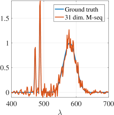
C.1.2. M-sequences
Maximal length sequences, or M-sequences for short, are optimal codes when using circular convolution. Their PSD is flat and hence is desirable as blur functions. However, since our convolution is linear, M-sequences are not necessarily the optimal choice.
C.2. Performance comparison
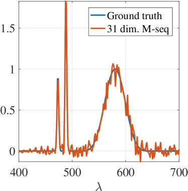
We compare optimized codes, spatially compact codes and M-sequ- ences for their performance in spatial deconvolution and spectral deconvolution. To test spectral deconvolution, we created a spectrum with two closely spaced narrowband peaks and a broadband peak, and blurred them with various codes. Readout noise and shot noise were added to adhere to real world measurements. Finally, deconvolution was done with wiener filter. To test spatial deconvolution, we used Airforce target and blurred with the scaled PSD of the pupil codes, and added noise. Deconvolution was done with a TV prior in all cases.
Figure 21 shows a comparison of performance for spectral and spatial deconvolution. As expected, optimized codes perform the best for spectral deconvolution, while spatially compact codes perform worse. Spatially compact codes perform the best in this case, while optimized codes come close. Since hyperspectral imaging requires good spatial as well as spectral resolution, we chose optimized codes.
C.3. Spectral deconvolution
Recall that our optical setup measures a blurred version of the true spectrum. Specifically, if the aperture code is and the spectrum to be measured is , our optical setup measures , where is additive white gaussian noise. The addition of noise prevents us from simply dividing in Fourier domain. Fortunately, since the aperture code was designed to be invertible, it is fairly robust to noise. A naive solution, such as Wiener deconvolution, hence, works very well. If the noise is too high, or the spectra is known to be smooth, we can impose an penalty on the difference and solve the following optimization problem:
| (29) |
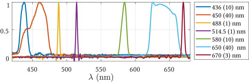
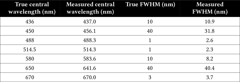
where is the measured spectrum, is the aperture code, is the spectrum to be recovered, and is the first difference of . Further priors, such as positivity constrains give better results as well. Figure 23 shows a comparison of spectra of various commonly available light sources, as well as a comparison with spectrometric measurements. We showed results for three forms of deconvolution, namely, Wiener deconvolution, regularized deconvolution, and positivity constrained deconvolution. Figure 22 shows results for some narrowband filters. We computed the central wavelength and Full Width Half Max (FWHM) for each filter and compared it against the numbers provided by the company. As expected, the FWHM of 1nm filters is between 2nm and 3nm, as the FWHM of our optical setup is 3nm. FWHM for 10nm filters and 40nm filters is close to the ground truth values.
C.4. Spatial deconvolution
The presence of a coded aperture introduces a blur in spatial domain, which is the scaled power spectral density of the coded aperture. Our optimization procedure accounts for invertible spectral blur as well as invertible spatial blur. Hence, deconvolution is stable even in the presence of noise. While naive deconvolution procedures such as Wiener deconvolution or Richardson-Lucy work well, we imposed total variance (TV) penalty on the edges to get more accurate results. Figure 24 shows blurred image of Siemen star, and deconvolution with TV-prior, Wiener and Richardson-Lucy algorithms. As with spectral deconvolution, spatial deconvolution is fairly robust to choice of algorithm. We chose TV-prior, as it returned the sharpest results. Figure 25 shows MTF before and after deconvolution, with TV-prior. Deconvolution signficantly improves the MTF30 value, which jumps from 20 line pairs/mm to 90 line pairs/mm.
Appendix D List of components
Figure 26 shows an annotated image of the optical setup we built along with a list of components along with their company and item number. The system was optimized for a central wavelength of 580nm and hence the relay arm till the diffraction grating has been tilted at with respect to the diffraction grating to correct for schiempflug. Lenses in the relay arm are tilted by with respect to the diffraction grating so that the objective can be aligned with the relay arm without any further tilt. The first beamsplitter (component 8) and the second turning mirror (component 10) have been placed on a kinematic platform to correct for misalignments in the cage system. It is of importance that we chose an LCoS instead of a DMD for spatial light modulation. The reasons:
-
•
Since the output after modulation by DMD is not rectilinear to the DMD plane, it introduces further scheimpflug, which is hard to correct.
-
•
DMD acts as a diffraction grating with Littrow configuration, as it is formed of extremely small mirror facets. This will introduce artifacts in measurements which are non-linear.
Some more design considerations are enumerated below:
-
(1)
Lenses. We used 100mm achromats for all lenses except the last lens before cameras. Achromats were the most compact and economical choice for our optical setup, while offering low spatial and spectral distortion.
-
(2)
Polarizing beam splitters. We used wire grid polarizing beamsplitters everywhere to ensure low dependence of spectral distortion on angle of incidence, and increase the contrast ratio.
-
(3)
Using an objective lens for measurement camera. Note that a lens is placed between the LCoS and measurement sensor which converts spatially-coded image to spectrum and coded spectrum to spatial image. Instead of using another achromat, we used an objective lens set to focus at infinity. Since objective lenses are free of any distortions, and are optimized to focus at infinity, this significantly improves resolution of measurements.
-
(4)
Diffraction grating. We used an off-the-shelf transmissive diffraction grating with 300 groves/mm, which offered most compact spectral dispersion without any overlap with higher orders. This ensured that there would be no spectral vignetting at any point in the setup. Further discussion about the choice of grove density is provided in section E
-
(5)
Polarization rotators. We bought off-the-shelf Liquid Crystal (LC) shutters and peeled off the polarizers on either sides to construct polarization rotators. This is the most economic option, while offering contrast ratios as high as 400:1. The key drawback is that the settling time is 330ms, which prevents their usage at very high rate. A natural workaround is to incorporate binary Ferroelectric shutters which have a low latency rate of 1ms. However, since ours was only a lab prototype, we decided to go with the cheaper option.
Appendix E Design considerations
We outline some design choices we made and the rationale behind them in this section.
E.1. Choice of code size
The pupil code has two free parameters, the length of the code and the pitch size . The two parameters control the invertibility of spectrum and imperceptibility of spatial images. To understand our design choices, we present constrains and physical dimensions of various measurements. Let each lens in the optical setup have a focal length and aperture diameter . Let pixel pitch of measurement camera be . This implies that the camera can capture all spatial frequencies up to . Let the size of grating be in each dimension and its grove density be .
We capture wavelengths from to . The grating equation is given by, , where is the groves spacing and is the order of diffraction, 1 in our case. Solving for angular spread of spectrum, we get, The size of spectrum then is . The minimum resolvable wavelength is . To avoid vignetting in a system, we require that the pupil plane be no larger than , giving us .
Recall that the pupil code is , where is the binary pupil code and . Using the formula for PSF of an incoherent system, we know that the Fourier transform of the PSF is , where is the linear autocorrelation of and is spatial frequency in . To capture all spatial frequencies, we need to be non-zero for , which gives us .
In our optical setup, we have , , , and , which leaves us , and as free variables. To prevent vignetting, we need to be less than , which means that N increases as decreases. Increasing increases resolution of images, but the optimization problem for optimal binary code becomes lengthy. On the other hand, increasing can increase spatial resolution, but the spectral resolution reduces. Keeping practical considerations in mind, we set , which took close to a day to optimize. Further, was the smallest grove density we obtained as off-the-shelf component.
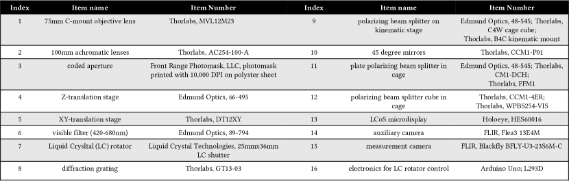
E.2. Handling positive/negative data
When computing singular vectors, the data to be measured, as well as the data to be displayed on the LCoS contains negative values. Since our optical devices cannot handle negative data, we make two positive measurements and combine them. We split the data to be displayed on the LCoS into positive and negative parts. Then, we capture positive data with positive part on the LCoS, and then repeat the process for negative data. By taking the difference of the positive and negative data, we obtain the required measurement. Figure 27 shows an example of capture of data with positive/negative data. The data in (a) shows the positive/negative image to be displayed on the LCoS, which is split into positive (b) and negative (c) halves, which are separately displayed on the LCoS, to capture positive (e) and negative (f) data. The final required measurement is then obtained by appropriately weighing and subtracting the two measurements.
Appendix F Calibration
We now outline calibration steps for the proposed optical setup. Firstly, we need a mapping between the captured image and the image displayed on the SLM. Secondly, we need calibration of wavelengths, and finally, we need spectral response calibration of the system for high-fidelity measurements.
Camera-SLM calibration.
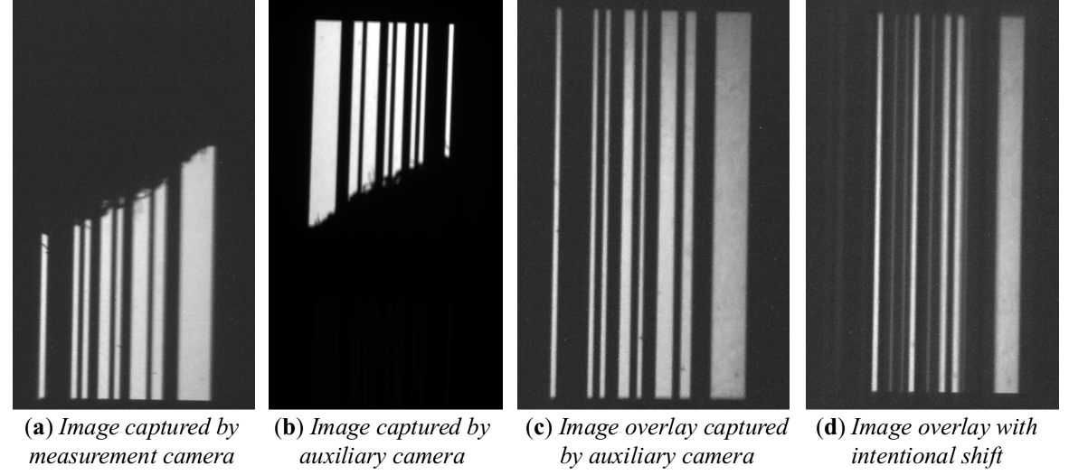
Recall that the power method for estimating eigen vectors requires the multiplication , where is a spatial measurement, displayed on the SLM and is the measurement made by the camera. Hence, we need a one-to-one mapping between the measured image and the LCoS. To do this, we added a second, calibration camera, henceforth called the auxiliary camera, which directly sees the image on the LCoS. The calibration steps are:
-
(1)
Find pixel to pixel correspondence between LCoS and auxiliary camera using gray or binary codes.
-
(2)
Place known target in front of the camera.
-
(3)
Capture the image of the target using the primary camera. Let this image be .
-
(4)
Capture the image of the target on the LCoS using second camera. Let this image be .
-
(5)
Register and using a similarity transform.
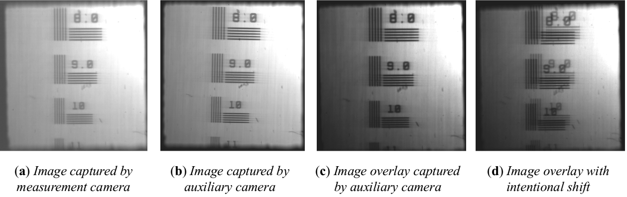
The steps are then repeated for the spectrum. Instead of placing a known target image, a narrow band filter is placed. This creates the coded aperture pattern on both the cameras. The image of the coded aperture for the narrow band filters can be used for registering the cameras for spectral measurements. For robustness, we combined images of two narrow band filters, namely 514.5nm with an FWHM of 1nm and 670nm with an FWHM of 3nm, which helped registration of the camera and LCoS over a larger field of view.
Figure 28 shows spatial and spectral calibration results. (a) shows the images of target captured by auxiliary camera and (b) shows capture by measurement camera. The calibration process was verified by displaying the captured target image back on the SLM and then capturing the image of LCoS by auxiliary camera. The result is shown in (c). (d) shows the result if the registration were not successful, showing ghosting of the two images. (e) and (f) show image of spectrum of a narrowband filter. Since the pupil code is vertically symmetric, we stuck a piece of tape at the bottom, creating a trapezoidal shape, which was then easy to register. (g) shows the overlay image captured by the auxiliary camera, for verification. A good registration results in an image that looks like the aperture code itself. (h) shows the result of an intentional shift, to show the effect of a bad registration. In both cases, we used Matlab’s built in SURF based automatic image registration technique for estimating a similarity transform between the two captured images.
Wavelength calibration.
Wavelength calibration requires two steps – 1) Estimating the binary code of the coded aperture and 2) Estimating locations of wavelengths. We found thresholding the measured spectrum to be a robust way of estimating the binary code of the coded aperture. To calibrate wavelength locations, we use three filters of known spectral response. Specifically, we use 488nm, 514.5nm and 670nm spectral filters with FWHM of 1nm, 1nm and 3nm respectively. Since spectral spread is linear, two known wavelengths are sufficient. However, for robustness, we use a third filter and then linearly interpolate to get the wavelength positions.
Figure 29 shows the image for wavelength calibration pipeline. We first obtain image of spectrum of a narrow band filter. After correcting for rotation, we obtain spectrum by summing the image vertically. This helps estimate the binary code, which is then used to deconvolve the observed spectrum to get spectrum of the narrow band filter. The peak of the narrow band filter is used as a known location. The process is then repeated for 488nm and 670nm filters to get wavelengths.
Spectral response of camera / Radiometric calibration.
The measured image and specturm on the camera plane is given by
where is the spectral response of the camera. For true spectrometric readings, contribution of needs to be removed. This can be achieved by calibrating the spectrometric measurements with a known light source. The tungsten-halogen light source, “SL1-CAL” from Stellarnet was used for this purpose. To compute , we assumed that the true spectrum, of the light source is known. We then measured spectrum of the light source, with our optical setup. The spectral response of the system was then computed as . This procedure is illustrated in Figure 30.
Appendix G Real experiments
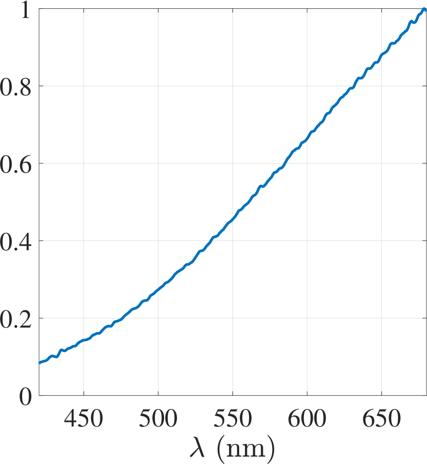
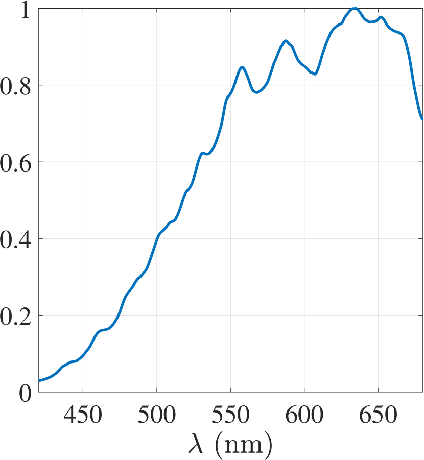
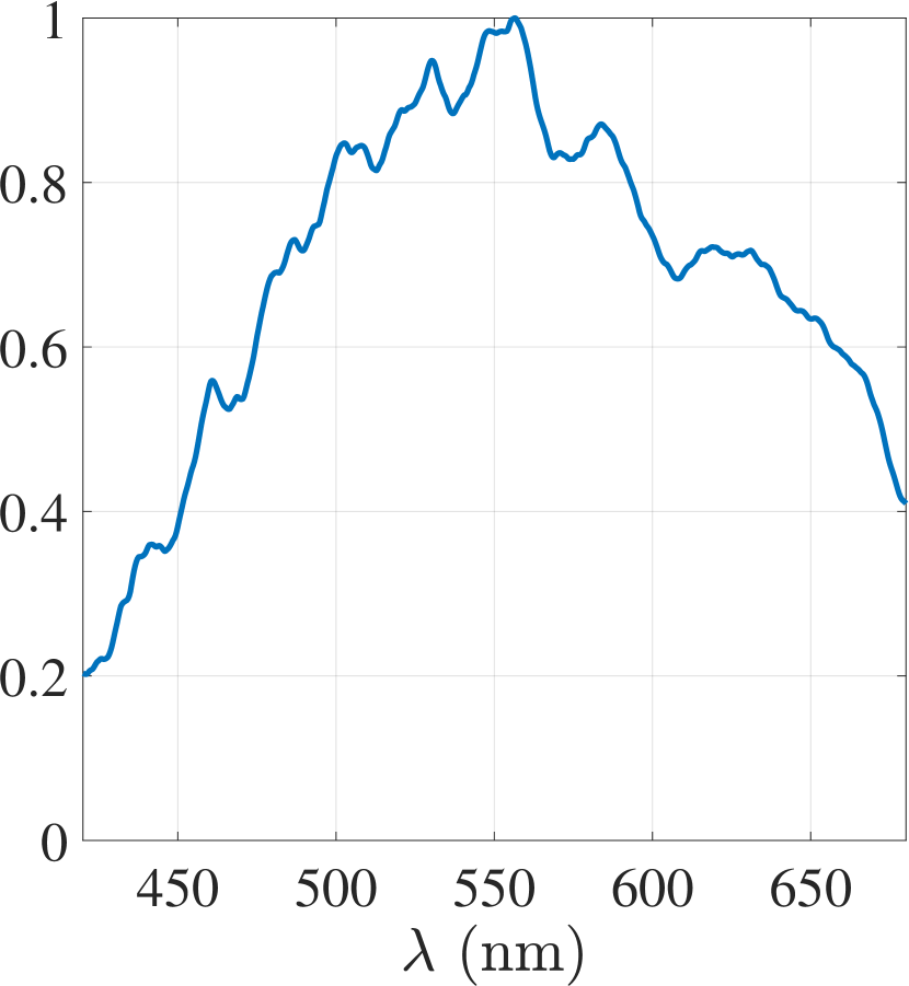
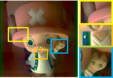
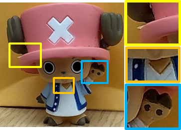
We provide visualizations for some of the real experiments presented in the main paper. Specifically, we compare the captured singular vectors for two scenes with spectrally Hadamard multiplexed measurements. We also show spectral band images for Macbeth chart and crayons chart, showing the intensity variation of various colors.
G.1. Visualizing spatial images
Figure 33 shows images across various wavelengths for the “color checker” scene and “crayons” scene. In particular, The images show the variation of intensity of each color swatch/crayon across wavelengths, with blur objects being brighter initially, green objects in the middle and red objects finally. Figure 31 shows RGB image captured by our lab prototype as well as a cellphone camera for the Chopper scene. The insets shows textured areas which show high spatial resolution of our prototype.
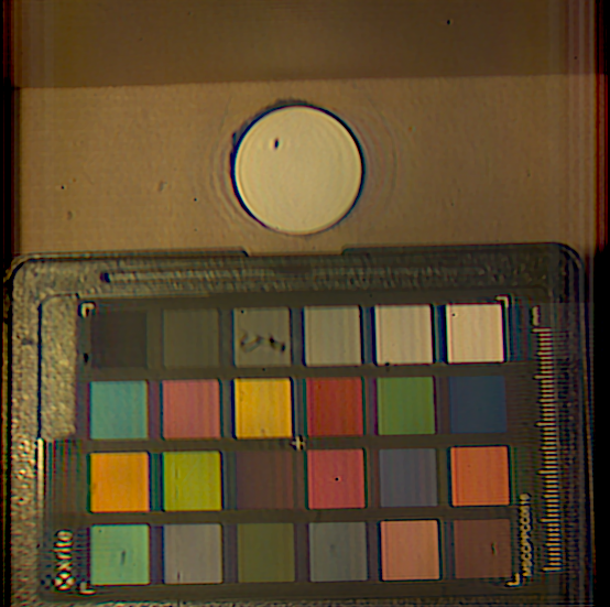
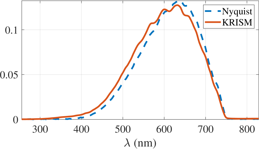
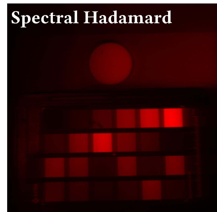

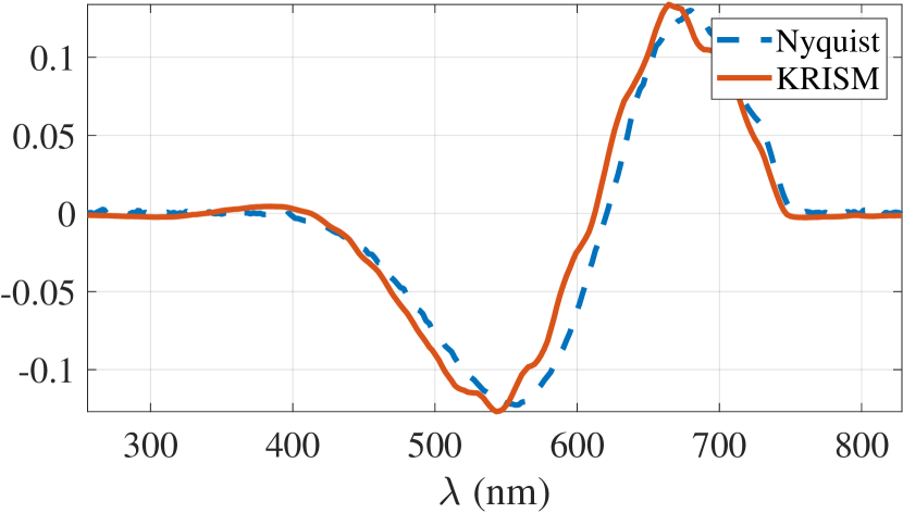
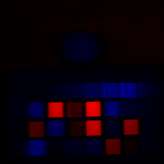
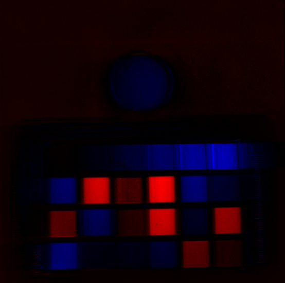
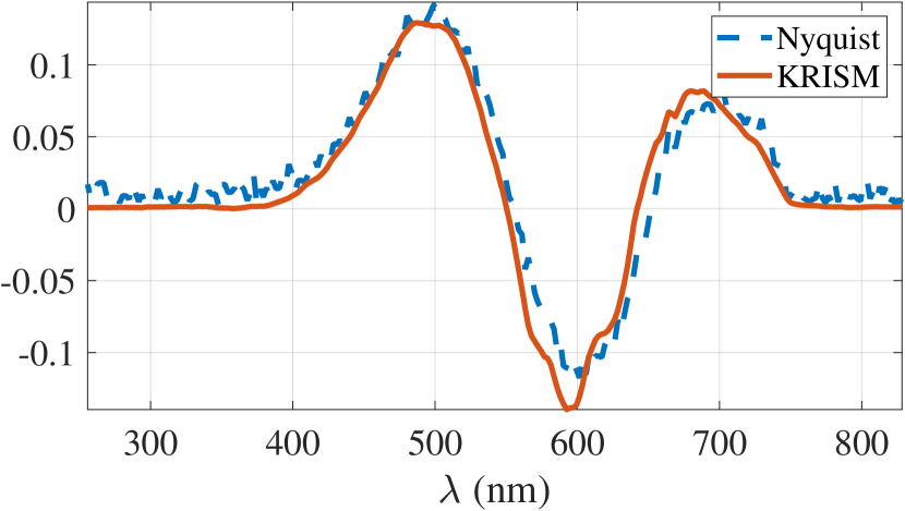
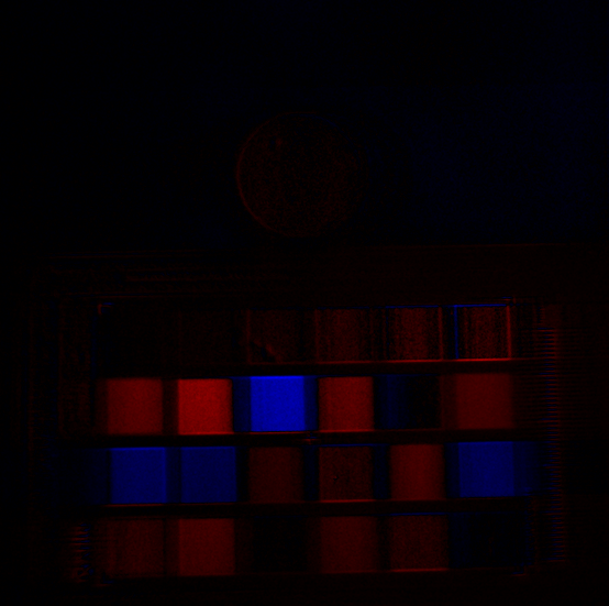
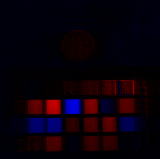

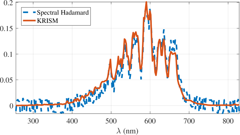


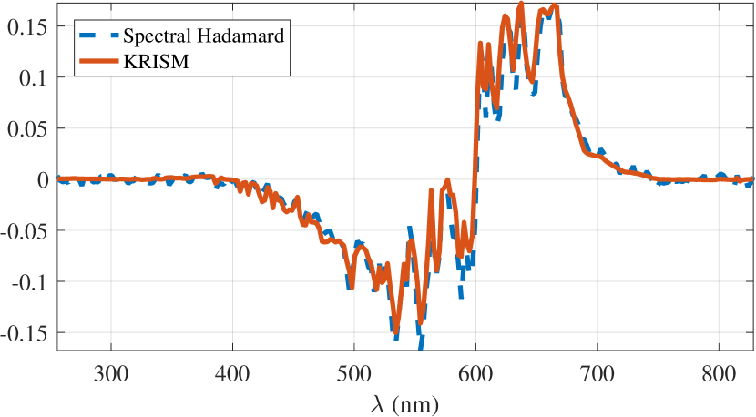
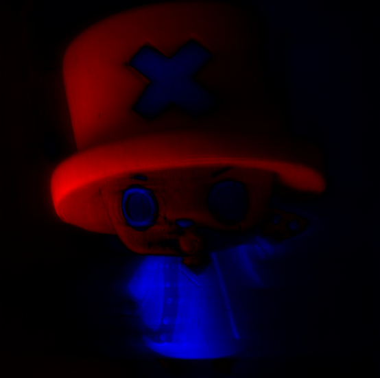
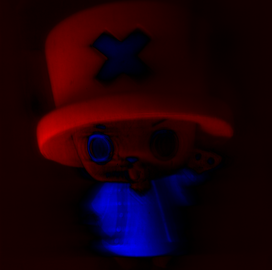
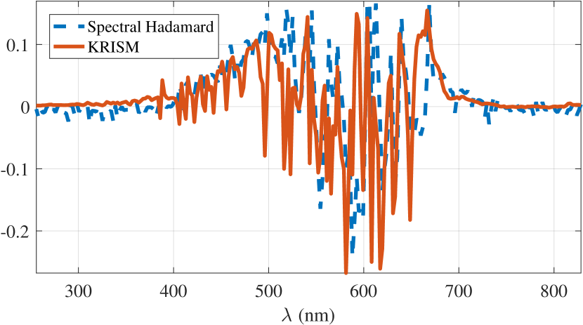
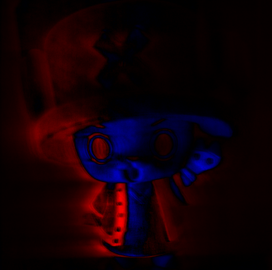
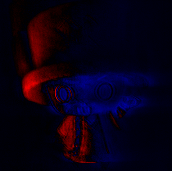
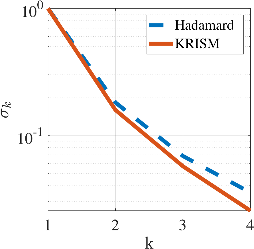
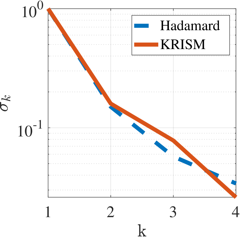
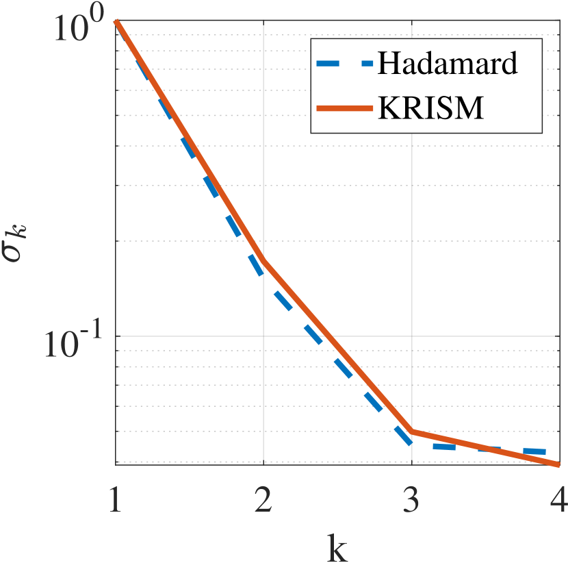
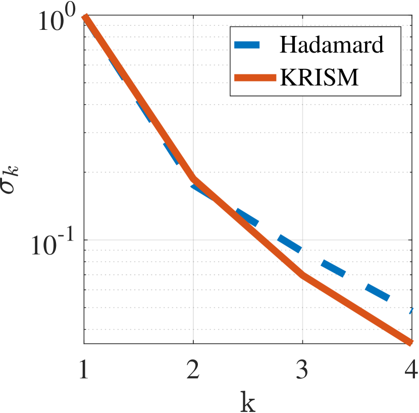
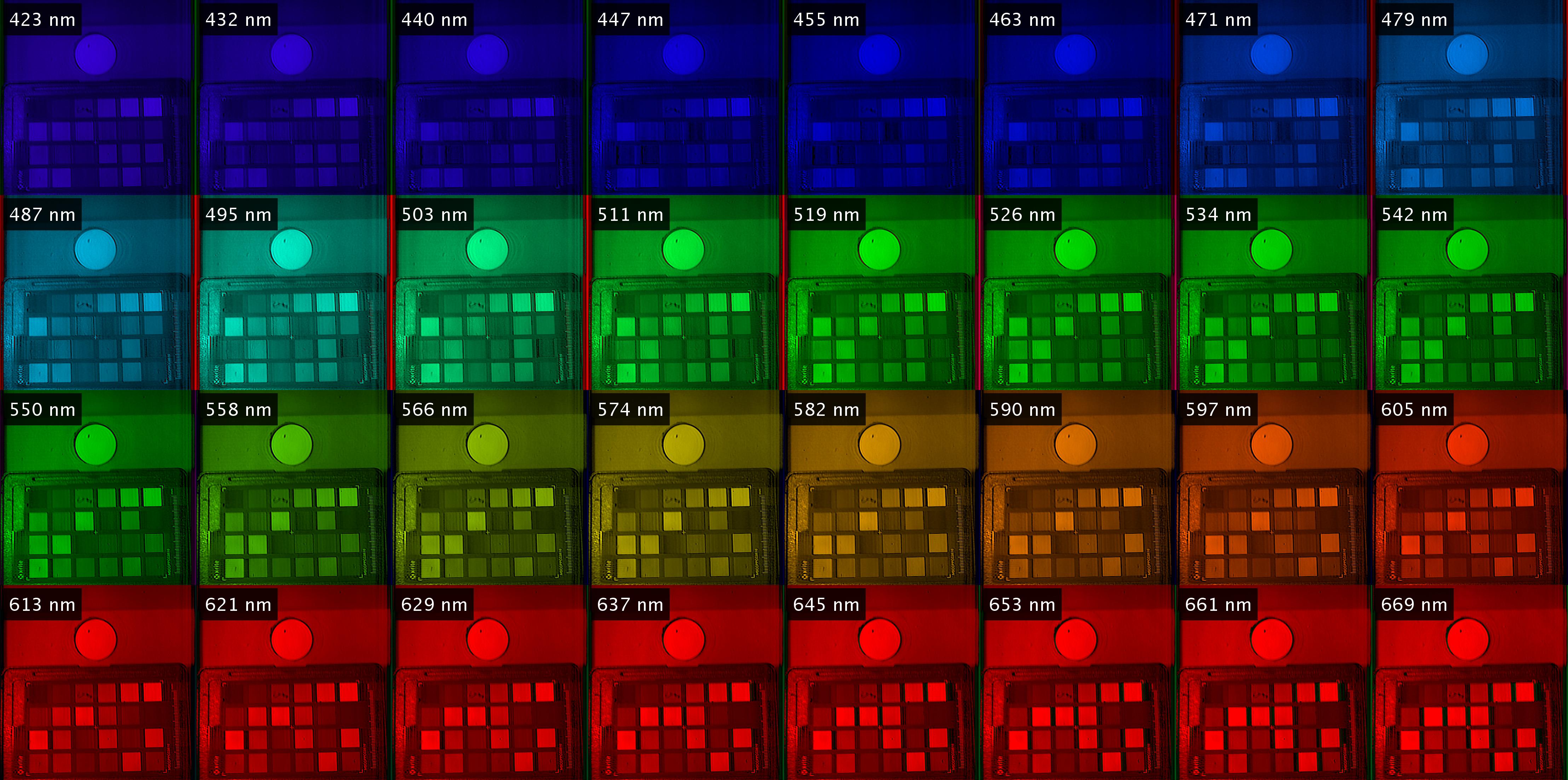
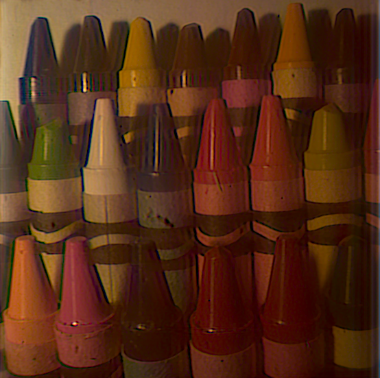
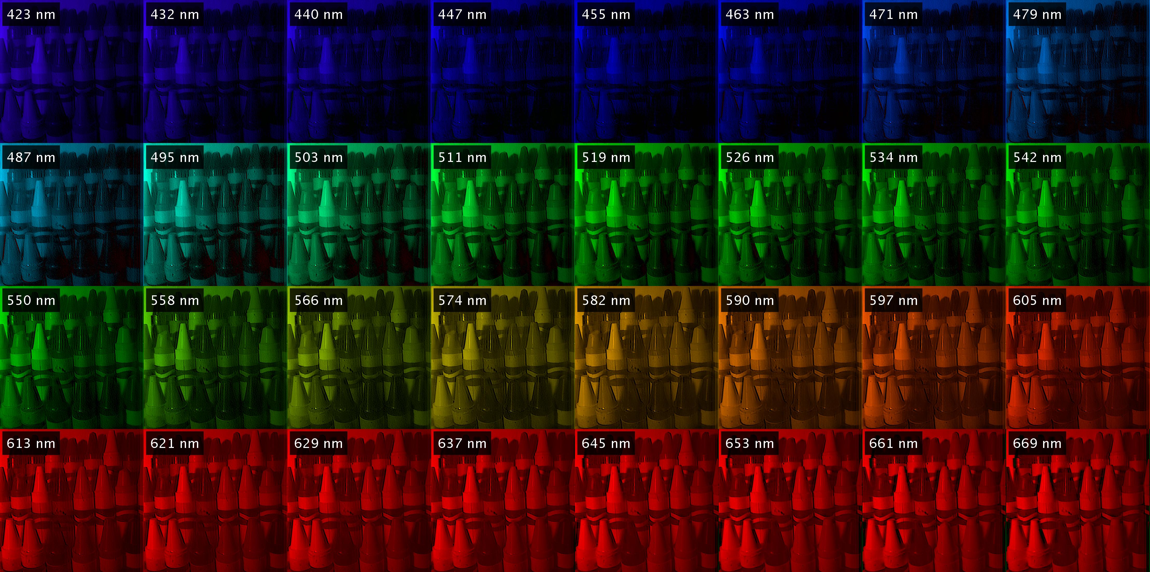
G.2. Comparison of singular values and singular vectors
The ability of KRISM to accurately compute singular vectors has been presented in the main paper. Here, we present two more experimental measurements to show how KRISM is applicable across various settings. Comparison is done against spectrally Hadamard multiplexed data, and then computing singular vectors on computer. We evaluate three metrics, namely, SNR between singular values, SAM between spectral singular vectors and SAM between spatial singular vectors. “Color checker” experiment (first row in Figure 32) was captured by placing the Macbeth chart in front of the camera, and illuminating with a tungsten-halogen light source. The PSNR between singular values was dB, average SAM between spectral singular vectors and that between spatial singular vectors was . “Chopper” experiment (second row in Figure 32) was captured by placing the Chopper toy in front of the camera, and illuminating it with CFL, a peaky illuminant. The PSNR between singular values was dB, average SAM between spectral singular vectors and that between spatial singular vectors was . Finally, the last row shows a comparison between singular values from Hadamard multiplexing and singular values from KRISM for some scenes presented in the main paper. Across the board, KRISM computes the low-rank approximation with very high accuracy, as is evident from the experiments.
Appendix H Synthetic experiments
We showed some simulation results in the main paper. We show several more examples here, with emphasis on diversity of datasets. We tested KRISM via simulations on four different datasets and compared it against competing techniques for hyperspectral imaging.
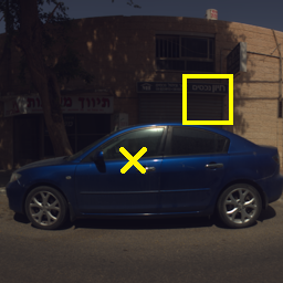
Ben-Shahar
()


PSNR: 38.6dB,

PSNR: 41.1dB,

PSNR: 40.3dB,

PSNR: 49.1dB,
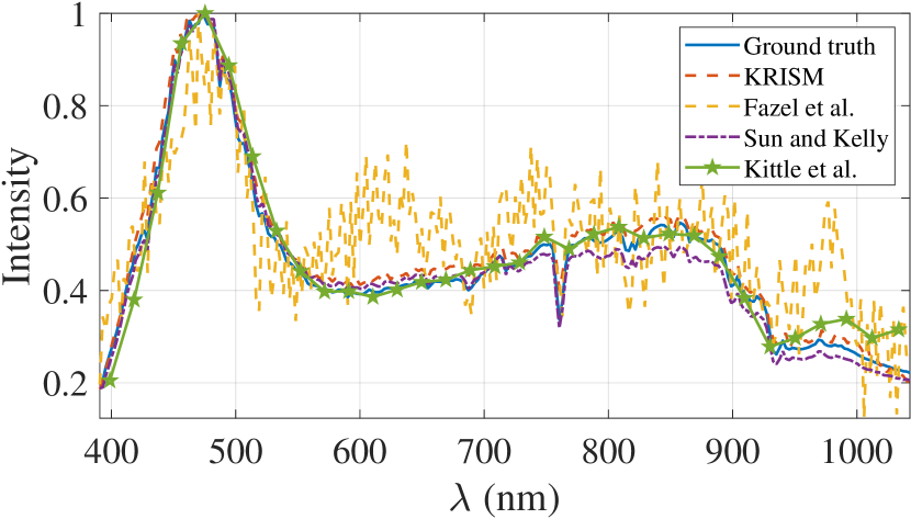
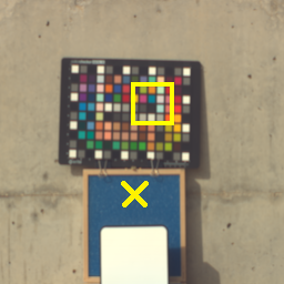
()


PSNR: 33.3dB,

PSNR: 34.0dB,

PSNR: 35.4dB,

PSNR: 39.9dB,
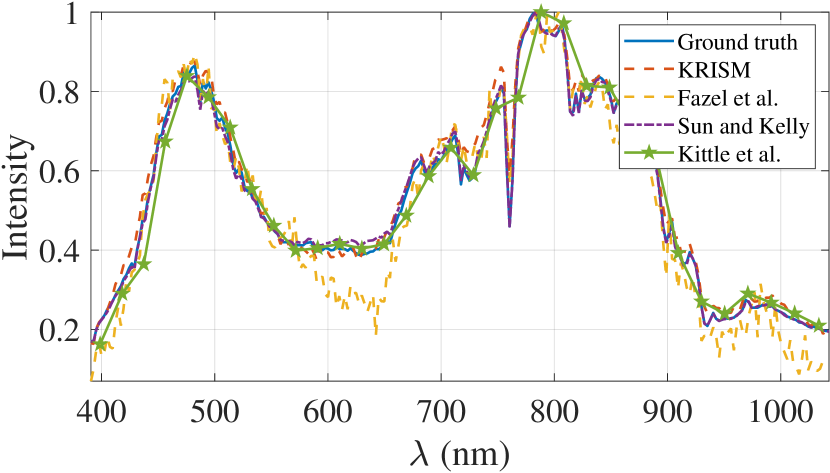
()


PSNR: 27.1dB,

PSNR: 30.1dB,

PSNR: 36.8dB,

PSNR: 44.1dB,
Datasets.
We used the hyperspectral data set by Arad and Ben-Shahar [2016] (ICVL dataset), which consists of several high spatial and spectral resolution hyperspectral images covering 519 bands in visible and near IR wavelengths. We downsampled the HSI to to keep computation with CASSI-type simulations tractable. We also used datasets from Choi et al. [2017]; Yasuma et al. [2010] and Chakrabarti and Zickler [2011] with 31 spectral bands to compare with learning-based techniques. Finally, we present one example from NASA AVIRIS to compare KRISM against Row/Column CS proposed in [Fazel et al., 2008].
Competing methods.
We compared KRISM against four competing CS hyperspectral imaging techniques. All methods were simulated with 60dB readout and photon noise and 12-bit quantization. Specifics of each simulation model are given below:
-
(1)
KRISM: We performed a rank-4 approximation of the HSI with 6 spatial and 6 spectral measurements. Diffraction blur due to coded aperture was introduced both in spectral and spatial profiles. Deconvolution was then done using Wiener deconvolution in both spectral and spatial domains.
-
(2)
Fazel et al. [2008]: As with KRISM, we performed a rank-4 approximation of the HSI by computing random Gaussian projections with 6 spatial and 6 spectral measurements. Diffraction blur due to coded aperture was introduced as well.
- (3)
- (4)
-
(5)
Kittle et al. [2010]: We used the multi-frame CASSI architecture for obtaining coded images, and recovered the HSI with sparsity prior in wavelet domain. We reduced the number of spectral bands for ICVL dataset to 31 to keep computations tractable.
-
(6)
Sun and Kelly [2009]: We obtained spatially-multiplexed spectral measurements with random permuted Hadamard matrix and recovered the HSI with sparsity in wavelet domain.
We define reconstruction SNR as , where is the Frobenius norm and is the recovered version of .

dB

dB

dB
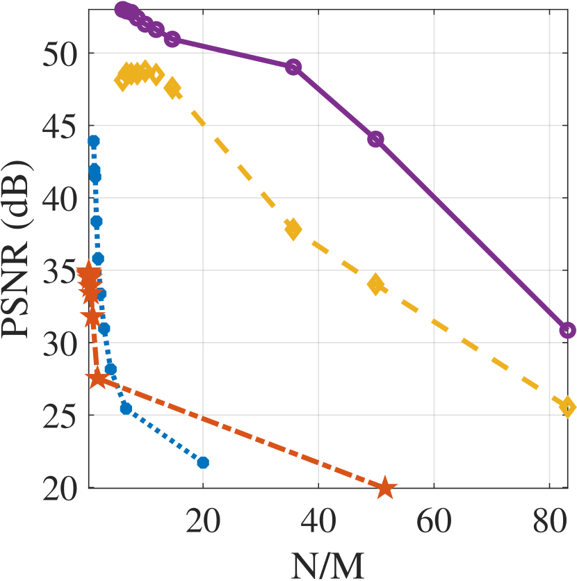
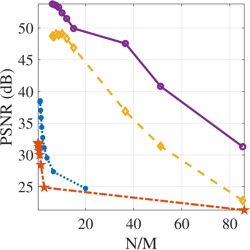
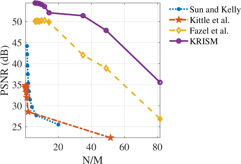

(25.9dB, )

(47.8dB, )
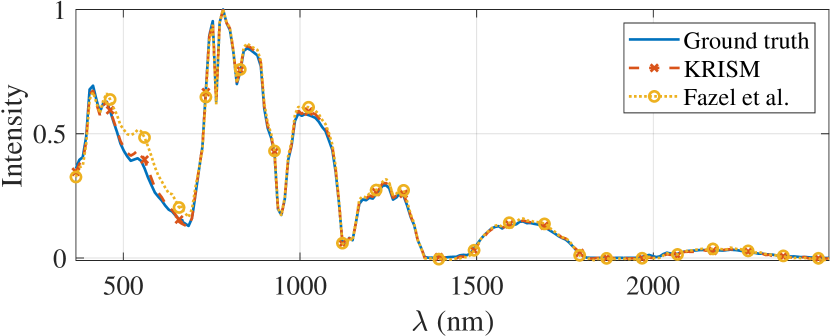
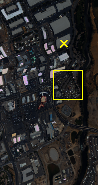

(41.3dB, )

(46.5dB, )
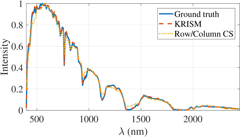
H.1. Performance with high spectral resolution
The true potential of KRISM can be exploited when there are a large number of spectral bands, such as the ones in the dataset by Arad and Ben-Shahar [2016]. We keep compression low for competing methods as the accuracy scaled poorly with higher compressions (see Figure 35) Results on some representative examples have been show in Figure 34. Qualitatively, the reconstructed spatial images as well as the spectral signatures are very close to ground truth. Figure 36 shows a comparison of reconstruction SNR as a function of compression ratios. As is evident, KRISM works significantly better than other methods despite very high compression ratios. The closes competitor to KRISM is the Row/Column CS approach by [Fazel et al., 2008]. We show comparison between KRISM and Row/Column CS on one example from NASA’s AVIRIS dataset consisting of of 224 spectral bands between 400-2400nm, and on SpecTIR [2019] dataset consisting of 178 spectral bands, making it a good example to test our method. Results are shown in Figure 38. For the same compression ration, KRISM offers a 10dB higher accuracy, and is qualitatively more accurate in both spatial images and spectral profiles.
H.2. Performance with low spectral resolution
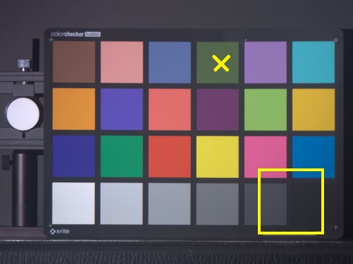
()

PSNR: 36.9dB,

PSNR: 32.9dB,
PSNR: 31.6dB,

PSNR: 32.5dB,

PSNR: 41.8dB,
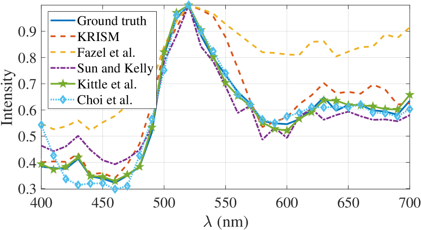
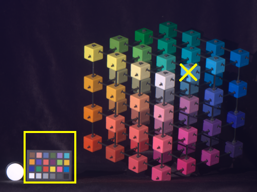
()

PSNR: 35.0dB,

PSNR: 32.4dB,
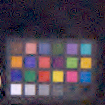
PSNR: 31.2dB,

PSNR: 30.6dB,

PSNR: 37.5dB,
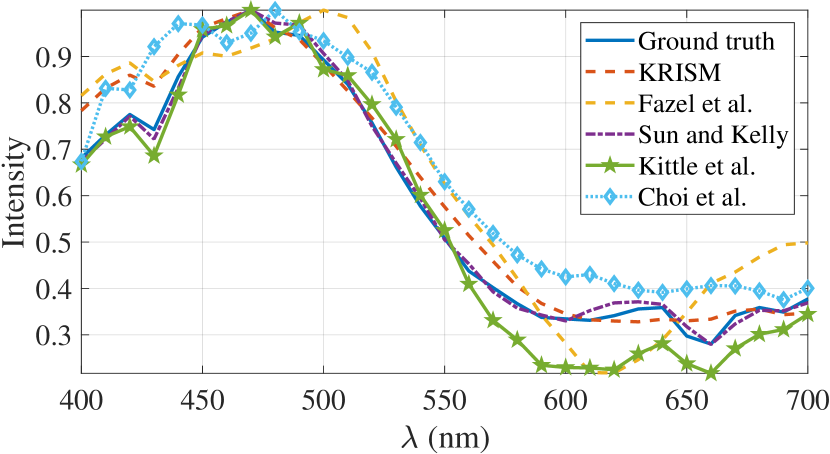
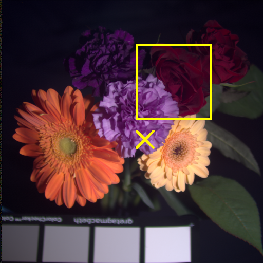
()

PSNR: 37.7dB,
PSNR: 35.2dB,
PSNR: 31.6dB,

PSNR: 40.6dB,

PSNR: 48.2dB,
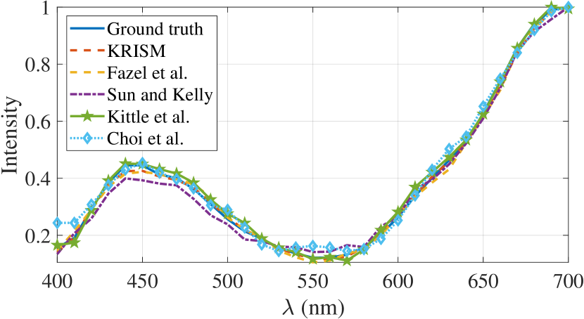
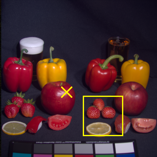
()
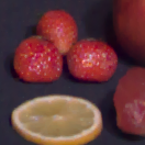
PSNR: 37.6dB,
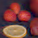
PSNR: 36.4dB,
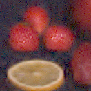
PSNR: 32.2dB,
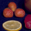
PSNR: 32.8dB,

PSNR: 41.2dB,
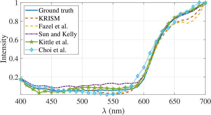
()
PSNR: 42.0dB,
PSNR: 38.9dB,

PSNR: 44.5dB,

PSNR: 45.6dB,

PSNR: 50.7dB,
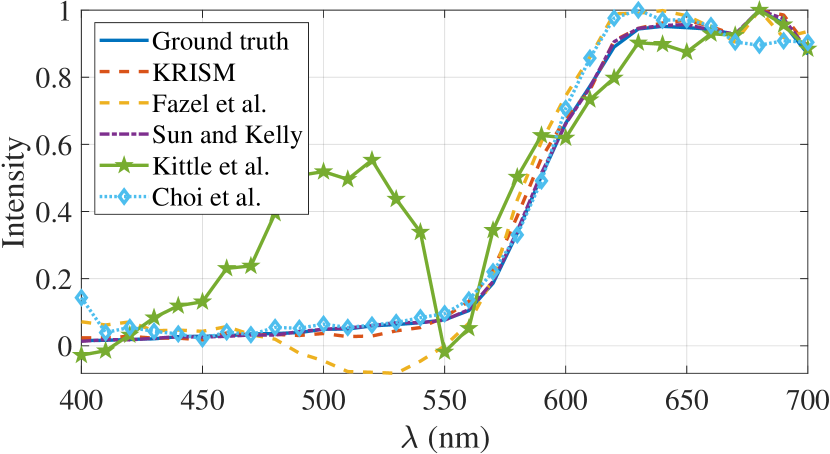
()

PSNR: 41.3dB,
PSNR: 36.0dB,
PSNR: 46.9dB,

PSNR: 47.9dB,

PSNR: 50.2dB,
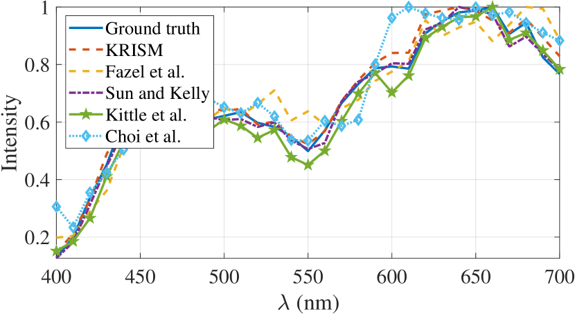
Most of the visible HSI datasets contains 31-33 spectral bands between 400 - 700nm. In this regime, learning-based snapshot techniques such as Choi et al. [2017] and [Lin et al., 2014a] have better performance. We used the dataset by Chakrabarti and Zickler [2011], Choi et al. [2017] and Yasuma et al. [2010] for simulations with 31 spectral bands. Spatial resolution has been specified for individual images in Figure 39. We compare KRISM with varying number of measurements against snapshot techniques [Choi et al., 2017; Lin et al., 2014a] in Figure 40. We observe that in the setting closest to snapshot mode, Choi et al. [2017] and Lin et al. [2014a] do outperform KRISM; this is to be expected since after a single iteration, KRISM provides only a rank-1 approximation. As the number of KRISM iterations are increased (which allows approximations of higher ranks), KRISM performance improves. We note that simulations for [Lin et al., 2014a] were performed with downsampled dataset and only on a select set of scenes as the recovery required several days for each scene even with parallelization. Figure 41 shows recovery SNR as a function of compression for multi-frame techniques. As was discussed in the main paper, KRISM is particularly effective for high resolution imaging. However, even with small number of bands, performance is superior in terms of spatial and spectral resolutions. It is worth noting that learning-based snapshot technique by [Choi et al., 2017] outperforms [Kittle et al., 2010] with fewer measurements. This is expected, as it exploits the smooth nature of underlying spectra.
()


,
PSNR: dB

,
PSNR: dB

,
PSNR: dB

,
PSNR: dB

,
PSNR: dB

,
PSNR: dB