Uncertainty Estimation in Functional Linear Models

Abstract Functional data analysis is proved to be useful in many scientific applications. The physical process is observed as curves and often there are several curves observed due to multiple subjects, providing the replicates in statistical sense. The recent literature develops several techniques for registering the curves and associated model estimation. However, very little has been investigated for statistical inference, specifically uncertainty estimation. In this article, we consider functional linear mixed modeling approach to combine several curves. We concentrate measuring uncertainty when the functional linear mixed models are used for prediction. Although measuring the uncertainty is paramount interest in any statistical prediction, there is no closed form expression available for functional mixed effects models. In many real life applications only a finite number of curves can be observed. In such situations it is important to asses the error rate for any valid statistical statement. We derive theoretically valid approximation of uncertainty measurements that are suitable along with modified estimation techniques. We illustrate our methods by numerical examples and compared with other existing literature as appropriate. Our method is computationally simple and often outperforms the other methods.

keywords Basis functions; B-splines; Bias correction; Estimating equations; Functional mixed models; Karhunen-Lo$\grave{e}$ve expansion; Prediction interval; Random effects;

1 Introduction

Functional data analysis received considerable attention in last couple of decades due to its applicability in various scientific studies (Ramsay and Silverman, 1997, 2010). A functional data consists of several functions or curves that are observed on a sufficiently large number of grid points. The dual characteristics of functional data, namely, maintaining the smoothness of individual curves through repeated observations and combining several curves poses the main challenge in functional data analysis (Morris and Carroll, 2006). In relatively simple situations where the curves could be represented by simple parametric models, this data characteristics can easily be handled by well established parametric mixed models (Laird and Ware, 1982, Verbeke and Molenbergs, 2000, Demidenko, 2013, McCulloch and Searle, 2001, Jiang 2007). In complex biological or physical processes, the parametric mixed models are not appropriate and thus modern functional mixed model techniques are developed. For a complete description and comparisons, instead of repeating the literature, we suggest Guo (2002a), Morris and Carroll (2006), Antoniadis and Sapatinas (2007), Chen and Wang (2011), Liu and Guo (2011), Maiti, Sinha and Zhong (2016) for recent developments in functional mixed linear models and their applications. Some of the related works, but not a complete list includes Brumback and Rice (1998), Goldsmith, Crainiceanu, Caffo and Reich (2011), Greven, Crainiceanu, Caffo and Reich (2011), Krafty, Hall and Guo (2011) and Staicu, Crainiceanu and Carroll (2010).

As noted by Antoniadis and Sapatinas (2007), much of the work done in this area is on estimation and only limited attention has been paid for inference. Morris and Carroll (2006) provided a comprehensive account of functional mixed models from Bayesian perspective. In Bayesian approach, the inference is automatic along with the estimation. However, this is not the case in frequentist perspective. Antoniadis and Sapatinas (2007) developed testing of random effects and fixed effects when a wavelet decomposition is used for smoothing the functional curves. They also observed the theoretical limitations of the procedures developed for functional mixed models, for example, Guo (2002a,b). Thus research developing theoretically valid inferential techniques for functional mixed models is important.

Prediction is one of the main objectives in functional data analysis in many applications. For example, one may like to predict the number of CD4 cells in HIV patients or thai circumference (related to body weight) for obese children in a future time point. The mixed effect, combination of fixed and random effects are typically used for such prediction. For statistical inference, standard error estimation of the mixed effects is an integral part of data analysis. However, this is a non trivial problem even in simple parametric random effect models. See, Kackar and Harville (1984), Rao and Molina (2015) and Jiang (2007) for various developments. We developed the approximation theory for standard error estimation as a measure of uncertainty for mixed effects in a functional linear mixed models. Our approach is frequentist. To our knowledge, the prediction error estimation in this sense for a functional mixed model is new. Guo (2002a) reported subject (curve) specific 95% confidence intervals in his applications. However, like Antoniadis and Sapatinas (2007) we were unable to verify the development with theoretical validation. We believe, Guo’s primary goal was in developing the functional mixed models and user friendly estimation rather than prediction interval estimation. This work, in this sense, is complementary to Guo (2002a) and an important contribution to the functional mixed model methodology.

In this paper we consider a functional mixed model similar to Chen and Wang (2011). We also follow the penalized spline smoothing technique similar to them. Of course there are other possible smoothing techniques, such as wavelet (Morris and Carroll, 2006, Antoniadis and Sapatinas (2007), functional principal components (Yao, Müller and Wang, 2005), Kauermann and Wegener, 2011 and Staicu, Crainiceanu and Carroll, 2010). For comparison, contrasts, computation and further literature review of various smoothing techniques in this context we refer to Chen and Wang (2011). The section 2 introduces the models and model estimation. The section also develops the approximation theory of prediction error. The simulation study and real data examples are given in Section 3. We conclude the development in Section 4. The proofs are deferred to Appendix.

2 Models and Estimation

We consider a functional mixed-effect model as

$$Y(t)=X(t)^{T}\beta(t)+Z(t)^{T}\nu(t)+e(t)$$ (2.1)

where $t\in(0,1)$, $\beta(t)$ is a $p$-dimensional fixed coefficient function, $\nu(t)$ is a $q$-dimensional subject-specific random coefficient functions and $e(t)$ is a Gaussian noise process with $e(t)\sim N(0,\sigma_{e}^{2})$ and $\hbox{cov}(e(t),e(s))=0$. We also assume that $e(t)$ and $\nu(t)$ are independent.

Let the data $\{Y(t_{ij}),X(t_{ij}),Z(t_{ij})\}$ are collected/designed at time points $t_{ij}$ for $i$-th subject, $i=1,\cdots,n$ and $j$-th time point, $j=1,\cdots,m_{i}$. Then the model (2.1) for this data is

$$Y(t_{ij})=X(t_{ij})^{T}\beta(t_{ij})+Z(t_{ij})^{T}\nu_{i}(t_{ij})+e_{ij}$$ (2.2)

where $X(t_{ij})=(X_{1}(t_{ij}),\cdots,X_{p}(t_{ij}))^{T}$ is the covariates, $Z(t)=(Z_{1}(t),\cdots,Z_{q}(t))^{T}$ known design for random effects $\nu_{i}(t)=(\nu_{i1}(t),\cdots,\nu_{iq}(t))^{T}$. These are zero mean Gaussian process with $Cov(\nu_{i}(t),\nu_{i}(s))=\gamma(t,s)$, a $q\times q$ positive definite matrix. We assume $\nu_{ik}(t)$ and $\nu_{jl}(t)$ are independent for $i\neq j$ or $k\neq l$. The objective is to obtain the mean square error for predicting the mixed effect $A=l^{T}_{0}\beta(t)+d^{T}_{0}\nu(t)$, where $l_{0}$ and $d_{0}$ are $p$ and $q$ dimensional known vectors.

Assume that $\beta_{k}(t),k=1,\cdots,p$ belongs to the normed space of continuous functions with finite second derivatives and the covariance $\gamma(s,t)$ can be decomposed by

$$\gamma(t,s)=B_{\nu k}(s)^{T}\Omega_{k}B_{\nu k}(s).$$

Then we can approximate $\beta_{k}(t)$ by

$$\beta_{k}(t)=B_{k}(t)^{T}\theta_{k}$$

where $B_{k}(t)=(B_{k1}(t),B_{k2}(t),\cdots,B_{kL}(t))^{T}$ is the vector of $L$ basis functions and $\theta_{k}=(\theta_{k1},\cdots,\theta_{kL})^{T}$ is the corresponding coefficients. By Karhunen-Lo$\grave{e}$ve expansion (Ash and Gardner, 1975), the random functions $\nu_{ik}(t)$ can be approximated by

$$\nu_{ik}(t)=B_{\nu k}(t)^{T}\alpha_{ik}$$

where $B_{\nu k}(t)=(B_{\nu k1}(t),\cdots,B_{\nu kL}(t))^{T}$, $\alpha_{ik}=(\alpha_{ik1},\cdots,\alpha_{ikL})^{T}$ and $\alpha_{i}$ are random coefficients with $\mbox{Var}(\alpha_{ik})=\Omega_{k}$. In this paper, we consider B-spline basis functions for $B_{k}(t)$ and $B_{\nu k}(t)$. Let $0=\tau_{0}<\tau_{1}<\cdots<\tau_{L_{0}}<\tau_{L_{0}+1}=1$ be a set of knot points and $\tau_{i}=\tau_{\min\{\max(i,0),L_{0}+1\}}$ for any $i=1-r,\cdots,L$, where $L=L_{0}+r$. Using these knots, we can define $L$ normalized B-spline basis function of order $r$. The B-spline basis is defined by

$$B_{ki}(t)=(\tau_{i}-\tau_{i-r})[\tau_{i-r},\cdots,\tau_{i}](\tau-t)_{+}^{r-1}\quad\mbox{for $i=1,\cdots,L$}$$

where

$$[\tau_{i-r},\cdots,\tau_{i}]\phi(\tau)=\frac{[\tau_{i-r+1},\cdots,\tau_{i}]\phi(\tau)-[\tau_{i-r},\cdots,\tau_{i-1}]\phi(\tau)}{\tau_{i}-\tau_{i-r}}$$

denotes the $r$-th order divided difference for $r+1$ distinct points $\tau_{i-r},\cdots,\tau_{i}$ of function $\phi$ and

$$[\tau_{j},\tau_{j+1}]\phi(\tau)=\frac{\phi(\tau_{j+1})-\phi(\tau_{j})}{\tau_{j+1}-\tau_{j}}.$$

If $\tau_{i}=\tau_{i+1}=\cdots=\tau_{i+m}$, then $[\tau_{i},\cdots,\tau_{i+m}]\phi(\tau)=\frac{\phi^{(m)}(\tau)}{m!}$ for some integer $m$. We also used B-spline for the $B_{\nu k}(t)$.

Then the model (2.2) is represented as a linear mixed effect model

$$Y_{i}=W_{i}\theta+U_{i}\alpha_{i}+e_{i}$$ (2.3)

where $Y_{i}=(Y(t_{i1}),\cdots,Y(t_{im}))^{T}_{m\times 1}$, $W_{i}=(W_{i1},\cdots,W_{im})^{T}_{m\times pL}$, $\theta=(\theta_{1}^{T},\theta_{2}^{T},\cdots,\theta_{p}^{T})^{T}_{pL\times 1}$, $U_{i}=(U_{i1},\cdots,U_{im})^{T}_{m\times qL}$ and $\alpha_{i}=(\alpha_{i1}^{T},\alpha_{i2}^{T},\cdots,\alpha_{iq}^{T})^{T}_{qL\times 1}$ with $W_{ij}=(W_{1}(t_{ij})^{T},\cdots,W_{p}(t_{ij})^{T})^{T}_{pL\times 1}$ and $U_{ij}=(U_{1}(t_{ij})^{T},\cdots,U_{q}(t_{ij})^{T})^{T}_{qL\times 1}$ where $W_{k}(t)=(X_{k}(t)B_{k1}(t),\cdots,X_{k}(t)B_{kL}(t))^{T}_{L\times 1}$ and $U_{k}(t)=(Z_{k}(t)B_{\nu k1}(t),\cdots,Z_{k}(t)B_{\nu kL}(t))^{T}_{L\times 1}.$ For convenience, denote $R_{i}=\mbox{Diag}(\sigma_{e}^{2},\cdots,\sigma_{e}^{2})$ as the variance of $e_{i}=(e_{i1},\cdots,e_{im})^{T}$. Define $\Omega=\mbox{Diag}\{\Omega_{1},\cdots,\Omega_{q}\}$. It follows that $\mbox{Var}(\alpha_{i})=\Omega$. Then, $\Sigma_{i}=U_{i}\Omega U_{i}^{T}+R_{i}$ is the variance of $Y_{i}$. Hence, we can write the mixed effect $A$ into a function of $\theta$ and $\alpha$, which is

$$A=l^{T}\theta+\sum_{i=1}^{n}d^{T}_{i}\alpha_{i}=l^{T}\theta+d^{T}\alpha$$ (2.4)

where $d=(d_{1}^{T},\cdots,d_{n}^{T})^{T}$ and

$$l=l_{0}^{T}\left(\begin{array}[]{ccc}B_{1}^{T}(t)&0&0\\ 0&\ddots&0\\ 0&0&B_{p}^{T}(t)\end{array}\right)\quad\mbox{and}\quad d_{i}=d_{i0}^{T}\left(\begin{array}[]{ccc}B_{\nu 1}^{T}(t)&0&0\\ 0&\ddots&0\\ 0&0&B_{\nu q}^{T}(t)\end{array}\right).$$

2.1 Estimation of the fixed parameter and random effects

Following Chen and Wang (2007), treating the random effect $\alpha_{i}$ as missing value, define the penalized joint log-likelihood for $Y_{i}$ and $\alpha_{i}$ as

$$\ell(\theta,\alpha) =\sum_{i=1}^{n}\{(Y_{i}-W_{i}\theta-U_{i}\alpha_{i})^{T}R_{i}^{-1}(Y_{i}-W_{i}\theta-U_{i}\alpha_{i})+\alpha_{i}^{T}\Omega^{-1}\alpha_{i}\}$$ (2.5)

$$\quad+\sum_{k=1}^{p}\lambda_{k}\theta_{k}^{T}\Delta_{\beta k}\theta_{k}+\sum_{k=1}^{q}\eta_{k}\sum_{i=1}^{n}\alpha_{ik}^{T}\Delta_{\nu ik}\alpha_{ik}$$

where $\Delta_{\beta k}=\int_{0}^{1}B_{k}^{(2)}(t)B^{(2)^{T}}_{k}(t)dt$, $B_{k}^{(2)}(t)$ is the second derivative of $B_{k}(t)$ with respect to $t$ and $\Delta_{\nu ik}$ are defined similarly based on the B-spline basis functions $B_{\nu k}(t)$.

Then (2.5) can be written as

$$\ell(\theta,\alpha) =\sum_{i=1}^{n}\{(Y_{i}-W_{i}\theta-U_{i}\alpha_{i})^{T}R_{i}^{-1}(Y_{i}-W_{i}\theta-U_{i}\alpha_{i})$$ (2.6)

$$+\alpha_{i}^{T}\Omega^{-1}\alpha_{i}\}+\theta^{T}\Delta_{\beta}\theta+\sum_{i=1}^{n}\alpha_{i}^{T}\Delta_{\nu i}\alpha_{i}.$$

where $\Delta_{\beta}=\mbox{Diag}\{\lambda_{1}\Delta_{\beta 1},\cdots,\lambda_{p}\Delta_{\beta p}\}$ and $\Delta_{\nu i}=\mbox{Diag}\{\eta_{1}\Delta_{\nu i1},\cdots,\eta_{q}\Delta_{\nu iq}\}$,

Given $\Omega$, the minimization of $\ell(\theta,\alpha)$ provides

$$\tilde{\theta} =(\sum_{i=1}^{n}W_{i}^{T}R_{i}^{-1}D_{i}W_{i}+\Delta_{\beta})^{-1}\sum_{i=1}^{n}W_{i}^{T}R_{i}^{-1}D_{i}Y_{i}$$

$$\tilde{\alpha}_{i} =(U_{i}^{T}R_{i}^{-1}U_{i}+\Omega^{-1}+\Delta_{\nu i})^{-1}U_{i}^{T}R_{i}^{-1}(Y_{i}-W_{i}\tilde{\theta}).$$

By some algebra, we then have

$$\tilde{\theta} = (\sum_{i=1}^{n}W_{i}^{T}\Sigma_{i}^{*}W_{i}+\Delta_{\beta})^{-1}\sum_{i=1}^{n}W_{i}^{T}{\Sigma_{i}^{*}}^{-1}Y_{i}$$ (2.7)

$$\tilde{\alpha} = \Omega^{*}U^{T}{\Sigma^{*}}^{-1}(Y-W\tilde{\theta})$$ (2.8)

where $\Sigma_{i}^{*}=U_{i}(\Omega^{-1}+\Delta_{\nu i})^{-1}U_{i}^{T}+R_{i}$ and $\Omega^{*}=\mbox{Diag}((\Omega^{-1}+\Delta_{\nu 1})^{-1},\cdots,(\Omega^{-1}+\Delta_{\nu n})^{-1})$.

Because $\Sigma^{*}$ involves some unknown parameters, we estimate the variance component $\sigma$ in $\Sigma^{*}$ by solving the following estimating equation

$$\mathcal{Q}_{VC,k}(\sigma):=-tr\{P\Sigma P\frac{\partial\Sigma^{*}}{\partial\sigma_{k}}\}+Y^{T}P\frac{\partial\Sigma^{*}}{\partial\sigma_{k}}PY=0\quad\mbox{for $k=1,\cdots,g$.}$$ (2.9)

where $P={\Sigma^{*}}^{-1}-{\Sigma^{*}}^{-1}W(W^{T}{\Sigma^{*}}^{-1}W+\Delta_{\beta})^{-1}W^{T}{\Sigma^{*}}^{-1}$. Notice that $\mathcal{Q}_{VC,k}(\sigma)$ contains $g$ estimating equations. Denote the estimate of $\sigma$ by $\hat{\sigma}$.

Note that the above estimating equation is bias-corrected score function from the score function of the restricted log-likelihood function. To see this point, we observe that restricted log-likelihood function is the following

$$\ell_{V}(\sigma) := -\hbox{log}|W{\Sigma^{*}}^{-1}W|-\hbox{log}(|\Sigma^{*}|)-(Y-W\tilde{\theta}-U\tilde{\alpha})^{T}R^{-1}(Y-W\tilde{\theta}-U\tilde{\alpha})$$ (2.10)

$$-\tilde{\alpha}^{T}\Omega^{-1}\tilde{\alpha}-\tilde{\theta}^{T}\Delta_{\beta}\tilde{\theta}-\tilde{\alpha}^{T}\Delta_{\nu}\tilde{\alpha}$$

$$= -\hbox{log}|W{\Sigma^{*}}^{-1}W|-\hbox{log}(|\Sigma^{*}|)-(Y-W\tilde{\theta})^{T}{\Sigma^{*}}^{-1}(Y-W\tilde{\theta})-\tilde{\theta}^{T}\Delta_{\beta}\tilde{\theta}$$

$$= -\hbox{log}|W{\Sigma^{*}}^{-1}W|-\hbox{log}(|\Sigma^{*}|)-Y^{T}PY.$$

Then the derivative of $\ell_{V}(\sigma)$ is

$$\frac{\partial\ell_{V}(\sigma)}{\partial\sigma}=-tr(P\frac{\partial\Sigma^{*}}{\partial\sigma_{k}})+Y^{T}P\frac{\partial\Sigma^{*}}{\partial\sigma_{k}}PY$$ (2.11)

But $E\{\frac{\partial\ell_{V}(\sigma)}{\partial\sigma}\}\neq 0$ unless $\Sigma^{*}=\Sigma$. To make the score equation to be unbiased, we modified the score function $\frac{\partial\ell_{V}(\sigma)}{\partial\sigma)}$ to be (2.9) such that it is unbiased.

2.2 Prediction and Prediction Mean Square Error

A naive prediction of $A$ given in (2.4) is $\tilde{A}(\sigma)=l^{\prime}\tilde{\theta}+d^{\prime}\tilde{\alpha},$ where $\sigma$ is an unknown vector of variance components in $\Sigma$. The $k$-th component of $\sigma$ will be denoted as $\sigma_{k}$ and $\sigma=(\sigma_{1},\cdots,\sigma_{g})^{T}$. Unlike the simple linear mixed models, this prediction is biased as stated in the following theorem.

Theorem 1

The prediction is biased and the bias of the prediction of $\tilde{A}(\sigma)$ is

$$\mbox{Bias}\{\tilde{A}(\sigma)\}=-l^{\prime}(W^{T}{\Sigma^{*}}^{-1}W+\Delta_{\beta})^{-1}\Delta_{\beta}\theta+d^{\prime}\Omega^{*}U^{T}{\Sigma^{*}}^{-1}W(W^{T}{\Sigma^{*}}^{-1}W+\Delta_{\beta})^{-1}\Delta_{\beta}\theta.$$ (2.12)

To reduce the order of bias, we propose a bias-corrected prediction for $A(\sigma)$ as

$$\tilde{A}_{c}(\sigma) =l^{\prime}\tilde{\theta}+d^{\prime}\tilde{\alpha}+l^{\prime}(W^{T}{\Sigma^{*}}^{-1}W+\Delta_{\beta})^{-1}\Delta_{\beta}\tilde{\theta}$$ (2.13)

$$\quad-d^{\prime}\Omega^{*}U^{T}{\Sigma^{*}}^{-1}W(W^{T}{\Sigma^{*}}^{-1}W+\Delta_{\beta})^{-1}\Delta_{\beta}\tilde{\theta}.$$

The proof is deferred to the Appendix.

Theorem 2

If $d=(d_{1}^{\prime},\cdots,d_{n}^{\prime})^{\prime}$ is sparse, namely only a finite number of $d_{j}$’s are non-zeros ($j=1,\cdots,n$). Then the bias of $\tilde{A}_{c}(\sigma)$ is of order $n^{-2}$, which is negligible in comparing to $n^{-1}$.

The proof is deferred to the Appendix.

Now we will derive the prediction error formula. Let $Q=\mbox{Diag}(Q_{1},\cdots,Q_{n})$ and $D=(W^{T}\Sigma^{-1}W)^{-1}(I+B(W^{T}\Sigma^{-1}W)^{-1})^{-1}B(W^{T}\Sigma^{-1}W)^{-1}$ where $Q_{i}=\Sigma_{i}^{-1}U_{i}\Omega(I+\Delta_{\nu i}\Omega-\Delta_{\nu i}\Omega U_{i}\Sigma_{i}^{-1}U_{i}\Omega)\Delta_{\nu i}\Omega U_{i}\Sigma_{i}^{-1}$ and $B=W^{T}QW+\Delta_{\beta}$. Define $\Delta_{1}=(W^{T}\Sigma^{-1}W)^{-1}W^{T}Q-DW^{T}(\Sigma^{-1}+Q)$. Then it can be shown that

$$E\{(\tilde{A}_{c}(\sigma)-A(\sigma))^{2}\} =(l-W^{T}s)^{T}(W^{T}\Sigma^{-1}W)^{-1}(l-W^{T}s)+d^{\prime}(\Omega-\Omega U^{\prime}\Sigma^{-1}U\Omega)d$$ (2.14)

$$+(l^{\prime}-s^{\prime}W)\Delta_{1}\Sigma\Delta_{1}^{T}(l^{\prime}-s^{\prime}W)^{T}$$

$$+2(l^{\prime}-s^{\prime}W)\Delta_{1}\Sigma(s^{\prime}+(l^{\prime}-s^{\prime}W)(W^{T}\Sigma^{-1}W)^{-1}W^{T}\Sigma^{-1})^{T}$$

$$-2(l^{\prime}-s^{\prime}W)\Delta_{1}U\Omega d^{\prime}+O(n^{-2})$$

where $s=d^{\prime}\Omega^{*}U^{T}{\Sigma^{*}}^{-1}$.

Let $B=(B_{1},\cdots,B_{g})$ and $J=(J_{1},\cdots,J_{g})^{T}$ where

$$B_{k}^{T} = -(s^{\prime}W-l^{\prime})(W^{T}{\Sigma^{*}}^{-1}W+\Delta_{\beta})^{-1}W^{T}{\Sigma^{*}}^{-1}\frac{\partial\Sigma^{*}}{\partial\sigma_{k}}{\Sigma^{*}}^{-1}W(W^{T}{\Sigma^{*}}^{-1}W+\Delta_{\beta})^{-1}W{\Sigma^{*}}$$

$$+(s^{\prime}W-l^{\prime})(W^{T}{\Sigma^{*}}^{-1}W+\Delta_{\beta})^{-1}W^{T}{\Sigma^{*}}^{-1}\frac{\partial\Sigma^{*}}{\partial\sigma_{k}}{\Sigma^{*}}^{-1}$$

$$-s^{\prime}\frac{\partial\Sigma^{*}}{\partial\sigma_{k}}{\Sigma^{*}}^{-1}(I-W(W^{T}{\Sigma^{*}}^{-1}W+\Delta_{\beta})^{-1}W{\Sigma^{*}}),$$

and $J_{k}^{T}=\theta^{T}\Delta_{\beta}(W^{T}{\Sigma^{*}}^{-1}W+\Delta_{\beta})^{-1}W^{T}{\Sigma^{*}}^{-1}\frac{\partial\Sigma^{*}}{\partial\sigma_{k}}+\theta^{T}WP\frac{\partial\Sigma^{*}}{\partial\sigma_{k}}P.$ Further, denote $(\lambda_{1},\cdots,\lambda_{g})^{T}:=D^{-1}B$ and $G_{i}=P\frac{\partial\Sigma^{*}}{\partial\sigma_{i}}P$. The following theorem states a practical formula for the $MSE\{\hat{A}_{c}(\hat{\sigma})\}$.

Theorem 3

The MSE of prediction $\hat{A}_{c}(\hat{\sigma})$ for $A(\sigma)$ is

$$MSE\{\hat{A}_{c}(\hat{\sigma})\}$$

$$=(l-W^{T}s)^{T}(W^{T}\Sigma^{-1}W)^{-1}(l-W^{T}s)+d^{\prime}(\Omega-\Omega U^{\prime}\Sigma^{-1}U\Omega)d+(l^{\prime}-s^{\prime}W)\Delta_{1}\Sigma\Delta_{1}^{T}(l^{\prime}-s^{\prime}W)^{T}$$

$$+2(l^{\prime}-s^{\prime}W)\Delta_{1}\Sigma(s^{\prime}+(l^{\prime}-s^{\prime}W)(W^{T}\Sigma^{-1}W)^{-1}W^{T}\Sigma^{-1})^{T}-2(l^{\prime}-s^{\prime}W)\Delta_{1}U\Omega d^{\prime}+2tr\{(BD^{-1}J\Sigma)^{2}\}$$

$$+tr^{2}(\Sigma BD^{-1}J)+tr(D^{-1}B^{T}\Sigma BD^{-1}\Sigma_{w})+4\sum_{j=1}^{g}\sum_{l=1}^{g}\lambda_{j}^{T}\Sigma(G_{j}\Sigma G_{j}+G_{l}\Sigma G_{j})\Sigma\lambda_{l}+o(n^{-1}),$$

where $D=\left(\frac{\partial\mathcal{Q}_{VC,k}(\sigma)}{\partial\sigma_{l}}\right)_{kl}$, $\tilde{e}=(e_{1},e_{2},\cdots,e_{g})^{T}$ and $e_{k}=Y^{T}P\frac{\partial\Sigma^{*}}{\partial\sigma_{k}}PY-tr(P\Sigma P\frac{\partial\Sigma^{*}}{\partial\sigma_{k}})$, and $\Sigma_{w}=(2tr(G_{i}\Sigma G_{j}\Sigma))_{i,j}$.

Therefore, an estimation of the $MSE\{\hat{A}_{c}(\hat{\sigma})\}$ can be obtained by plugging in the variance components estimate $\hat{\sigma}$ from (2.9) into the MSE expression.

2.3 Choice of smoothing parameters

As mentioned earlier, the basic modeling framework considered in this article is similar to Chen and Wang (2011), however, there is differences in smoothing procedure of fixed and random effects and in parameter estimation. We followed their smoothing parameter choices. For completeness we explained the procedure here briefly.

Chen and Wang (2011) proposed to estimate the variance component in $R$ by minimizing the following penalized log-likelihood, for given $\theta$ and $\alpha$,

$$\ell_{v}(\sigma)=\hbox{log}|R|+(Y-W\theta-U\alpha)^{T}R^{-1}(Y-W\theta-U\alpha)+\theta^{T}\Delta_{\beta}\theta+\alpha^{T}\Delta_{\nu}\alpha.$$ (2.15)

Decomposing each $W_{k}^{T}(t)=(W_{k(1)}^{T}(t),W_{k(2)}^{T}(t))^{T}$ and let $W_{k(1)}^{T}(t)$ be the first $r$ component of the $W_{k}^{T}(t)$ and $W_{k(2)}^{T}(t)$ be the rest $L_{0}$ component of $W_{k}^{T}(t)$. Now collecting $W_{(1)}^{T}(t)=(W_{1(1)}^{T}(t),\cdots,W_{p(1)}^{T}(t))$ be a $pr$ components vector and $\theta_{(1)}$ be the corresponding coefficients. The smoothing parameter $\lambda=(\lambda_{1},\cdots,\lambda_{p})^{T}$ are chosen by minimizing the following marginal REML

$$\ell_{m}(\lambda)=\hbox{log}|\Sigma_{\lambda}|+(Y-W_{(1)}\theta_{(1)})^{T}\Sigma^{-1}_{\lambda}(Y-W_{(1)}\theta_{(1)})+\hbox{log}|W_{(1)}^{T}\Sigma^{-1}_{\lambda}W_{(1)}|$$ (2.16)

where $\Sigma_{\lambda}$ is the marginal covariance of $Y$, which is

$$\Sigma_{\lambda}=R+U\Omega U+V_{(2)}$$

where $V_{(2)}=\sum_{k=1}^{p}V_{k(2)}$, $V_{k(2)}=\lambda_{k}^{-1}W_{k(2)}^{T}W_{k(2)}$ and $W_{k(2)}=(W_{k(2)}(t_{11}),\cdots,W_{k(2)}(t_{nm}))^{T}$.

The smoothing parameters $\eta=(\eta_{1},\cdots,\eta_{q})^{T}$ are chosen by minimizing the following marginal log-likelihood, for given $\alpha=\hat{\alpha}$

$$\ell_{m}(\eta)=\hbox{log}|R|+(Y-W\theta-U\alpha)^{T}R^{-1}(Y-W\theta-U\alpha)+\alpha^{T}\Delta_{\nu}\alpha+\hbox{log}|H|-\hbox{log}|\Delta_{\nu}|.$$

where

$$H=\frac{1}{2}\frac{\partial^{2}\ell_{v}(\sigma)}{\partial\alpha\partial\alpha^{T}}=U^{T}R^{-1}U+\Delta_{\nu}$$

for any symmetric matrix $\Delta_{\nu}$. Because $|\Delta_{\nu}|=\prod_{i=1}^{n}\prod_{k=1}^{q}\eta_{k}^{L}|\Delta_{\nu ik}|$, taking derivative of $\ell_{m}(\eta)$ with respect to $\eta_{k}$, gives

$$\sum_{i=1}^{n}\alpha_{ik}^{T}\Delta_{\nu ik}\alpha_{ik}+tr(H^{-1}\tilde{\Delta}_{\nu}^{(k)})-\frac{L}{\eta_{k}}=0$$

where $\tilde{\Delta}_{\nu}^{(k)}=\mbox{Diag}\{\tilde{\Delta}_{\nu 1}^{(k)},\cdots,\tilde{\Delta}_{\nu n}^{(k)}\}$ and $\tilde{\Delta}_{\nu i}^{(k)}=\mbox{Diag}\{0,0,\cdots,\Delta_{\nu ik},\cdots,0\}$ for $i=1,\cdots,n$. Then

$$\hat{\eta}_{k}=L\,{\left(\sum_{i=1}^{n}\alpha_{ik}^{T}\Delta_{\nu ik}\alpha_{ik}+tr(H^{-1}\tilde{\Delta}_{\nu}^{(k)})\right)}^{-1}.$$

3 Numerical Findings

We investigated the finite sample performance of the proposed method through simulation and real data examples. The simulation study is also designed to verify the asymptotic behavior of the approximated prediction error formula and and related coverage errors.

3.1 Simulation Study

We considered the following mixed model setup

$$Y(t_{ij})=X(t_{ij})\beta(t_{ij})+Z(t_{ij})\nu(t_{ij})+\epsilon(t_{ij})\quad\mbox{$i=1,\cdots,n$ and $j=1,\cdots,m_{i}$}$$ (3.17)

where $m_{i}=1$ for all $i=1,...,n$. Three different values of $n$ was chosen, 50, 100 and 200. We generated the time points $t_{ij}$ independently from Uniform(0,1). Let $X(t_{ij})=1+0.5t_{ij}+e_{ij},Z(t_{ij})=(0.1)\,\left(-(0.8415/2)+\sin(t_{ij})+u_{ij}\right),\beta(t_{ij})=2\,\cos(t_{ij})$. Set $e_{ij}\sim N(0,0.5^{2})$ and $u_{ij}\sim N(0,0.4^{2})$. We simulated $\nu(t)$ from a Gaussian process with mean 0 and covariance $\hbox{cov}(\nu(t_{i}),\nu(t_{j}))=B^{T}_{t_{i}}\,\rho^{|i-j|}\,B_{t_{j}}$ where $\rho=0.4$, and $\epsilon(t_{ij})$ from a Gaussian process with mean zero and $\hbox{cov}(\epsilon(t),\epsilon(s))=\sigma_{\epsilon}^{2}\,\delta_{st}$, where $\delta_{st}=1$ if $s=t$, and $0$ otherwise. We set $\sigma_{\epsilon}=1$. We call this set up as Case I. As a second case, we kept everything same except the covariance structure of the random effects. Specifically, we took $\hbox{cov}(\nu(s),\nu(t))=\rho^{|s-t|}$ with $\rho=0.4$. We call this as Case II. We also examined the performance for more fluctuated mean function where $\beta(t_{ij})=\cos(2\pi t_{ij})$. We call this as case III.

The main purpose of this simulation study is to evaluate the performance of mean square error of the predictor of mixed effects that measuring subject (curve) specific means. For example, we considered $A_{i}=\bar{X}_{i}\beta(t_{0})+\bar{Z}_{i}\nu_{i}(t_{0}),i=1,\cdots,n$ where $t_{0}$ is one of the time points $t_{ij}$ (for example $t_{11}$), and $\bar{X}_{i}$ and $\bar{Z}_{i}$ are means of $X_{ij}$ and $Z_{ij}$ respectively. In particular, here $p=1$ and $q=1$, $l_{0}=\bar{X}_{i}$ and $d_{i0}=\bar{Z}_{i}$ and rest of $d_{j0}=0$ for $j\neq i$. Similar to Chen and Wang (2007), we used the following algorithm to estimate $\beta,\alpha,\Omega$ and $\sigma$. We fixed the tuning parameters $\lambda$ and $\eta$ and set an initial value of $\Omega_{(0)}=\mbox{Diag}\{1,\cdots,1\}$, $\sigma^{2}_{\epsilon(0)}=1$, $\Omega^{*}_{(0)}=(\Omega_{(0)}^{-1}+\Delta_{\nu})^{-1}$ and $\Sigma_{i(0)}^{*}=U_{i}(\Omega^{-1}_{(0)}+\Delta_{\nu i})^{-1}U_{i}^{T}+\sigma^{2}_{\epsilon}I$. Then the initial estimates of $\alpha$ and $\theta$ are

$$\tilde{\alpha}_{(0)}=\Omega^{*}_{(0)}U^{T}{\Sigma^{*}}^{-1}_{(0)}(Y-W\tilde{\theta}_{(0)})\;\;\mbox{and}\;\;\tilde{\theta}_{(0)}=(\sum_{i=1}^{n}W_{i}^{T}\Sigma_{i(0)}^{*}W_{i}+\Delta_{\beta})^{-1}\sum_{i=1}^{n}W_{i}^{T}{\Sigma_{i}^{*}}^{-1}_{(0)}Y_{i}.$$

respectively. We then repeat the following steps until all the parameter estimates converge

• Step 1: estimate $\sigma^{2}_{\epsilon}$ through the estimating equation given in (2.9).

• Step 2: estimate $\tilde{\theta}$ and $\tilde{\alpha}$ through (2.7) and (2.8), and $\hat{\Omega}$ by

  $$\hat{\Omega}=\frac{1}{n}\sum_{i=1}^{n}\left\{\tilde{\alpha}_{i}\tilde{\alpha}_{i}^{T}+\hat{\Omega}^{*}-\hat{\Omega}^{*}U_{i}^{T}M_{i}U_{i}\hat{\Omega}^{*}\right\}$$

  where $M_{i}=\hat{\Sigma}_{i}^{-1}-\hat{\Sigma}_{i}^{-1}W_{i}(\sum_{i=1}^{n}W_{i}^{T}\hat{\Sigma}_{i}^{-1}W_{i}+\Delta_{\beta})^{-1}W_{i}\hat{\Sigma}_{i}^{-1}$.

Plugging in the estimates of $\theta,\alpha,\sigma_{\epsilon}$ and $\Omega$ from the previous algorithm, obtain a biased corrected estimation of $\hat{A}$ by $\tilde{A}_{c}(\sigma)$ given in (2.13).

We then compute the following three quantities:

• The true MSE: computed by $\frac{1}{K}\sum_{k=1}^{K}(\hat{A}_{i}^{(k)}-A_{i}^{(k)})^{2},i=1,\cdots,n$ where $K$ is the number of replicated data sets and $\hat{A}_{i}^{(k)}$ is the prediction of $A_{i}^{(k)}$ in the $k$-th replicate. In all cases we took $K=600$ replication.

• Estimate MSE with estimated variance components: computed by the formula given in (2.14) using estimated $\sigma$ and $\Omega$.

Along with the mean square prediction errors, we calculated 95% prediction coverage error where the prediction interval was calculated as $\widehat{A}\,\pm\,2\,{(\mbox{estimated}\,\,\mbox{MSE})}^{1/2}$.

The reported values in the table 1 are the averages of the prediction coverage over all the individuals. The relative bias is the relative difference between the true MSE and the estimated MSE, averaged over replications and then averaged over the individuals. Numbers in the bracket are the standard errors averaged over all the subjects.

Table 1: Output under the proposed method. The computation time for cases I, II and III are 37498, 52698 and 42659 sec respectively.

n	$\widehat{\sigma_{\epsilon}}$	Prediction Coverage	Relative Bias	True MSE
Case I:
50	0.9915(0.1034)	0.9454(0.0044)	0.0509(0.0325)	0.1015(0.0215)
100	0.9936(0.0732)	0.9488(0.0051)	0.0749(0.0365)	0.0599(0.0126)
200	0.9968(0.0521)	0.9558(0.0062)	0.0460(0.0332)	0.0222(0.0048)
Case II:
50	0.9918(0.1043)	0.9431(0.0058)	0.0560(0.0342)	0.1024(0.0217)
100	0.9937(0.0733)	0.9453(0.0059)	0.0859(0.0385)	0.0608(0.0129)
200	0.9971(0.0521)	0.9503(0.0067)	0.0383(0.0312)	0.0229(0.0050)
Case III:
50	0.9919(0.1042)	0.9426(0.0067)	0.0599(0.0356)	0.1029(0.0218)
100	0.9941(0.0734)	0.9575(0.0057)	0.0969(0.0392)	0.0616(0.0131)
200	0.9974(0.0521)	0.9660(0.0064)	0.0431(0.0345)	0.0236(0.0051)

In summarizing the tables, the performance of prediction error estimation is very satisfactory. The relative bias in prediction error is less than 10%. Both the prediction coverage and confidence coverage are fairly close to the nominal level.

3.2 Comparison with Guo (2002a)

Guo (2002a) reported prediction intervals based on Wahba (1983). In this section, we compare the numerical performance of the proposed method with Guo (2002a) in terms of subject specific prediction intervals. For this purpose, we considered the same model (3.17) with $m_{i}=6$ for all $i=1,...,n$, and $n$ was chosen as 25 and 50. We took, $X(t_{ij})=(4.5)e^{i/n},Z(t_{ij})=(0.1)e^{-i/n},\beta(t_{ij})=\cos(2\pi t_{ij})$. We set $\sigma_{\epsilon}=0.14$ for $n=25$ but changed to $0.12$ for $n=50$ to keep the signal-to-noise ratio comparable. Then we predicted the response at the time points $t_{ij}$ and calculated coverage and length of the prediction intervals under both the methods. For Guo (2002a), we used the SAS code provided by Liu and Guo (2011). Since the SAS code takes considerable longer time compared to our MATLAB code, we used only $K=100$ replicates in this comparison. The table (2) reported numerical values that were averaged over all individuals.

The 3rd and 4-th column correspond to the proposed method where as the 5-th and 6-th columns are correspond to Guo (2002a). The proposed method clearly outperform both the coverage and length of the prediction intervals. The coverage under proposed method is closed to the nominal level whereas that is about only 50% under Guo (2002a). The length of prediction interval under Guo (2002a) is about twice compared to the proposed method. However, in terms of prediction bias, both the methods are nicely comparable. Although the performance of the proposed method is remarkable in terms of prediction error, we like to re-iterate Guo (2002a)’s original development was not meant for prediction error, rather model estimation. Thus the result is not completely unexpected. Furthermore, the numerical study indicates the importance of the development of uncertainty measures under the frequentist approach. Since the numerical difference is remarkable, we explain below how the quantities are calculated, for clarification.

For fixed time point $t$, we wish to predict the quantity $A_{ij}$ for individual $i$ in replication $j$. Note that the number of individuals and replications here are denoted by $n$ and $K$, respectively. Denote the predicted value by $\widehat{A_{ij}}$. Then we derived the prediction intervals under each methods as described above. Denote this intervals by $I_{ij}$. Then for a time point $t$, we calculated the following:

$$\mbox{Prediction Coverage}(t) = \frac{1}{nK}\sum_{i=1}^{n}\sum_{j=1}^{K}\delta_{I_{ij}}(A_{ij})$$

$$\mbox{Length}(t) = \frac{1}{nK}\sum_{i=1}^{n}\sum_{j=1}^{K}\mbox{length}(I_{ij})$$

$$\mbox{Prediction Bias}(t) = \frac{1}{nK}\sum_{i=1}^{n}\sum_{j=1}^{K}\left|{\displaystyle{A_{ij}-\widehat{A_{ij}}\over A_{ij}}}\right|$$

where $\delta_{A}(b)=1$ if $b\in A$, and $0$ otherwise.

Table 2: Comparison of the proposed method with Guo (2002a) in terms of prediction intervals

n	time	Pred Cov	Length	PredBias	PredCov(Guo2002a)	Length(Guo2002a)	PredBias(Guo02a)
25	0.9420	0.9000	0.0850	0.0152	0.4919	0.1677	0.0150
	0.4491	0.9464	0.0893	0.0151	0.4238	0.1495	0.0153
	0.5752	0.9536	0.0912	0.0164	0.4119	0.1491	0.0166
	0.0965	0.9572	0.0871	0.0171	0.507	0.1837	0.0173
	0.9437	0.9124	0.0865	0.0150	0.5065	0.1684	0.0150
	0.7573	0.9664	0.0911	0.8821	0.4508	0.1520	1.0050
50	0.9420	0.9706	0.0705	0.0130	0.4624	0.138	0.0269
	0.4491	0.9740	0.0675	0.0124	0.38	0.112	0.0269
	0.5752	0.9780	0.0769	0.0134	0.38	0.111	0.0279
	0.0965	0.972	0.0688	0.0144	0.48	0.146	0.0284
	0.9437	0.9680	0.0714	0.0129	0.45	0.138	0.0265
	0.7573	0.9710	0.0693	0.7034	0.39	0.115	0.8857

3.3 Real Data Examples

In this section, we apply the proposed method to two real data sets for illustration.

Example 1. We considered the case study of lung function (FEV1) from a longitudinal epidemiologic study (Fitzmaurice, Laird and Ware, 2012). 1 to 7 seven repeated measurements on FEV1 were taken on each of the 133 (sampled) subjects aged 36 or older. Fitzmaurice et al. (2012) argued for a cubic polynomial mean model for regressing FEV1 on smoking behaviors. An appropriateness of a varying coefficient model can be tested by comparing the following two models.

$$H_{0} : Y(t)=X(t)\theta_{0}+Z(t)v(t)+\epsilon(t)$$

$$H_{1} : Y(t)=X(t)\theta_{0}+\sum_{l=1}^{L}X(t)B_{l}(t)\theta_{l}+Z(t)v(t)+\epsilon(t)$$

This equivalently testing the hypothesis

$$H_{0}:\theta_{1}=...=\theta_{L}=0$$

The test statistics here is

$$T_{n}=2\,\hbox{log}{\displaystyle{\mbox{likelihood }H_{1}\over\mbox{likelihood }H_{0}}}$$

This is asymptotically a Chi squared random variable with $L$ degrees of freedom under $H_{0}$. For our case $T_{n}=700.5114-684.0968=16.4146$, which gives the p–value $0.0116934$ when $L=6$. This justifies a functional model such as (3.17).

The Figure (1) presented the predicted curves and their 95% prediction intervals for the first 25 individuals. The fit seems reasonable. The table (3) reported the prediction coverage of the proposed method compared to Guo (2002a) in all the time points. For a fixed time point, the prediction coverages were calculated by checking the proportion of subject specific intervals cover the true value.

Table 3: Prediction coverage and length for FEV1 data

time points	PredCov	PredCov(Guo)	Length	Length(Guo)	PredBias	PredBias(Guo)
1	1	0.9167	0.7033	0.5242	0.0004	0.0361
2	0.8115	0.7705	0.2902	0.4183	0.0001	0.0411
3	0.8974	0.7692	0.4480	0.3730	0.0003	0.0418
4	0.9739	0.8000	0.6778	0.3700	0.0001	0.0496
5	0.9273	0.8455	0.4547	0.3892	0	0.0407
6	0.9278	0.8969	0.4210	0.4200	0.0001	0.0404
7	1	0.9510	0.7400	0.5559	0.0009	0.0395
averages	0.934	0.85	0.5335	0.4358	0.0003	0.0413

Figure 1: FEV1 data: red and green: prediction band by Guo2002a. purple and light blue: proposed prediction band

Example 2. We consider another data example of modeling blood concentrations of cortisol as considered by (Guo, 2002a). There were 22 patients, 11 with fibromyalgia (FM) and 11 normal (the plot in Guo (2002a) showed 24 patients, 12 on each group) and their blood samples were observed every hours over a 24 hours period of time. The objective is to model concentration of cortisol on FM patients. Guo (2002a) argued for a functional model for this data set. We fit our model and came to the similar conclusion that the FM group has significantly higher cortisol. Figure (4) shows the subject specific prediction along with the prediction intervals.

Figure 2: Cortisol data: top: patient group. down: control group. 12 graphs for each.

Figure 3: Cortisol data with prediction bands: top: patient group. down: control group.

Table 4: prediction coverage for Cortisol data

t	PredCov	PredCov(Guo2002a)	Length	Length(Guo2002a)	PredBias	PredBias(Guo2002a)
1	0.9167	0.625	8.4782	4.9302	0.0369	0.1469
2	0.8333	0.75	7.1589	4.0079	0.0372	0.1729
3	0.7500	0.5417	7.0751	3.5531	0.0358	0.2998
4	0.7500	0.5	7.2737	3.2912	0.0381	0.1999
5	0.9167	0.625	7.2601	3.1525	0.0347	0.1960
6	0.8750	0.7083	7.1888	3.0972	0.0356	0.1976
7	0.8750	0.5417	7.3709	3.0870	0.0294	0.3102
8	0.8750	0.6667	7.7112	3.0953	0.0327	0.2156
9	0.9167	0.6667	7.8958	3.1079	0.0335	0.2630
10	0.8750	0.6667	7.8527	3.1186	0.0371	0.2315
11	0.8750	0.4583	7.6627	3.1258	0.0334	0.5396
12	0.9583	0.875	7.4458	3.1293	0.0357	0.2083
13	0.8750	0.7083	7.2942	3.1293	0.0300	0.4598
14	0.9167	0.8333	7.1945	3.1257	0.0319	0.2549
15	0.8750	0.75	7.0657	3.1185	0.0251	0.6692
16	0.8750	0.7083	6.8582	3.1079	0.0253	0.3263
17	0.7083	0.7083	6.6018	3.0956	0.0120	0.8806
18	0.8333	0.5417	6.4041	3.0880	0.0326	0.9020
19	0.8333	0.625	6.3144	3.0996	0.0368	0.5168
20	0.8750	0.5833	6.2544	3.1571	0.0362	0.2335
21	0.8333	0.7083	6.1151	3.2987	0.0355	0.2823
22	0.7917	0.4167	5.9236	3.5648	0.0386	0.2051
23	0.8333	0.625	6.1485	4.0283	0.0369	0.2029
24	0.9130	0.4783	7.9552	4.9665	0.0355	0.1972
averages	0.8575	0.6380	7.104	3.395	0.03319	0.3380

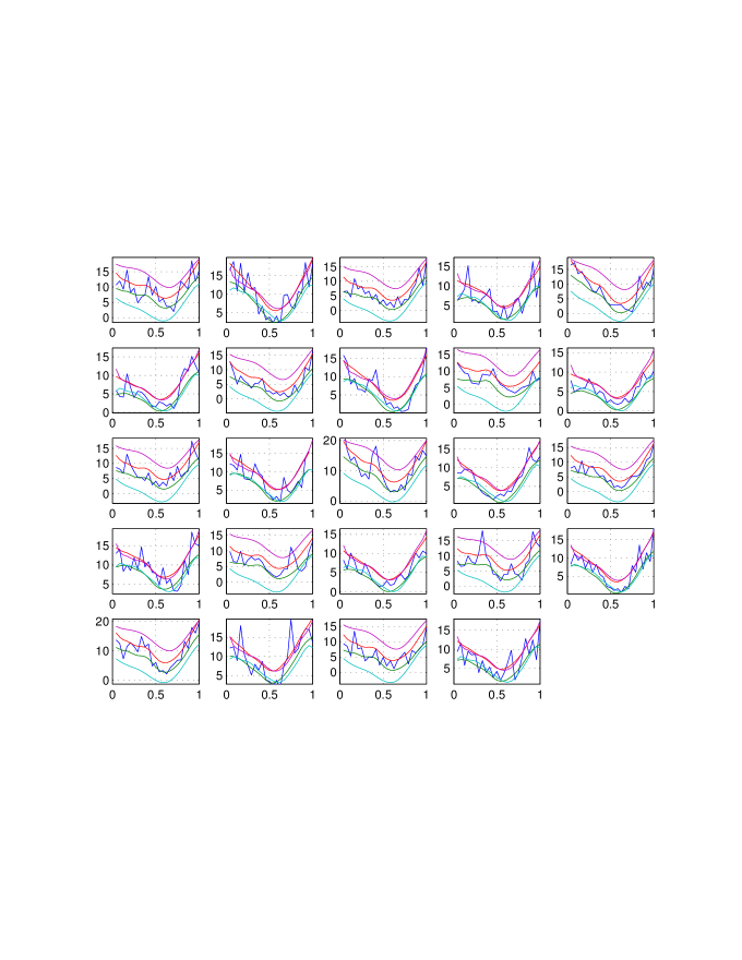
Figure 4: Cortisol data: red and green: prediction band by Guo2002a. purple and light blue: proposed prediction band

4 Discussion

The main motivation of this paper is to develop computationally simple yet theoretically valid uncertainty estimation in the context of individualized prediction using functional data. Although our approach is bias-corrected plug-in method, there could be additional bias due to plug-in the estimated parameters. It is possible to achieve further accuracy, however, that might introduce additional variability on the estimated uncertainty, thus the resulting formulas may loose their practicality. Nevertheless, the corrections we develop here are highly satisfactory as the maximum relative bias is less than 10%. The theoretically valid calculation of prediction intervals could be a dunting task in this context. However, if we simply apply the naive $\pm$ two standard type formula where the standard error formula is theoretically validated, the empirical coverage probabilities and the prediction lengths are much more improved than previously reported values.

The proposed method is implemented in MATLAB. Most of the computations of the proposed method can be handled easily due to the closed form solutions derived here. However, there are two parts which need numerical approximations, and high percentage of computation time in the method is due to these two optimization components. The first one is estimating the variance components $\sigma$ in the $Q$ function by finding its root as mentioned in the equation (2.9). This part is programmed in MATLAB using the function “fzero”. The second part is to estimate the tuning parameters $\lambda$ as the minimizer of the function $\l_{m}(\lambda)$ stated in the equation (2.16). The optimization function “fminbnd” in MATLAB is utilized to perform this numerical approximation. In contrast, Liu and Guo (2011) have developed a SAS code to implement their method. The computation time for their developed macro “fmixed” is considerably higher than our MATLAB code. This might be due to the differences between the optimization method used in our code and the ones utilized in “PROC MIXED”.

Appendix A

A.1 Proofs

In this Appendix, we provide technical proofs to Theorems in the paper.

Proof of Theorem 1: By definition, $\tilde{\theta}=(\sum_{i=1}^{n}W_{i}^{T}\Sigma_{i}^{*}W_{i}+\Delta_{\beta})^{-1}\sum_{i=1}^{n}W_{i}^{T}{\Sigma_{i}^{*}}^{-1}Y_{i}$ and $\tilde{\alpha}=\Omega^{*}U^{T}{\Sigma^{*}}^{-1}(Y-W\tilde{\theta})$ Then

$$\tilde{\theta}-\theta =-(\sum_{i=1}^{n}W_{i}^{T}\Sigma_{i}^{*}W_{i}+\Delta_{\beta})^{-1}\Delta_{\beta}W_{i}\theta+(\sum_{i=1}^{n}W_{i}^{T}\Sigma_{i}^{*}W_{i}+\Delta_{\beta})^{-1}\sum_{i=1}^{n}W_{i}^{T}{\Sigma_{i}^{*}}^{-1}(U_{i}\alpha_{i}+e_{i})$$

and

$$\tilde{A}(\sigma)-(l^{T}\theta+d^{T}\alpha) =-l^{\prime}(\sum_{i=1}^{n}W_{i}^{T}\Sigma_{i}^{*}W_{i}+\Delta_{\beta})^{-1}\Delta_{\beta}\theta$$

$$\quad+l^{\prime}(\sum_{i=1}^{n}W_{i}^{T}\Sigma_{i}^{*}W_{i}+\Delta_{\beta})^{-1}\sum_{i=1}^{n}W_{i}^{T}{\Sigma_{i}^{*}}^{-1}(U_{i}\alpha_{i}+e_{i})$$

$$\quad+d^{\prime}\Omega^{*}U^{T}{\Sigma^{*}}^{-1}(Y-W{\theta})+d^{\prime}\Omega^{*}U^{T}{\Sigma^{*}}^{-1}W(\theta-\tilde{\theta})-d^{T}\alpha.$$

After taking expectation, it is easy to see the conclusion.

Proof of Theorem 2: From the derivation in Theorem 1, it is easy to see that the bias of $\tilde{A}_{c}(\sigma)$ is

$$E\{\tilde{A}_{c}(\sigma)-\tilde{A}(\sigma)\} =l^{\prime}(\sum_{i=1}^{n}W_{i}^{T}\Sigma_{i}^{*}W_{i}+\Delta_{\beta})^{-1}\Delta_{\beta}E(\tilde{\theta}-\theta)$$

$$-d^{\prime}\Omega^{*}U^{T}{\Sigma^{*}}^{-1}W(W^{T}{\Sigma^{*}}^{-1}W+\Delta_{\beta})^{-1}\Delta_{\beta}E(\tilde{\theta}-\theta).$$

$$=-l^{\prime}(\sum_{i=1}^{n}W_{i}^{T}\Sigma_{i}^{*}W_{i}+\Delta_{\beta})^{-1}\Delta_{\beta}(\sum_{i=1}^{n}W_{i}^{T}\Sigma_{i}^{*}W_{i}+\Delta_{\beta})^{-1}\Delta_{\beta}W_{i}\theta$$

$$+d^{\prime}\Omega^{*}U^{T}{\Sigma^{*}}^{-1}W(W^{T}{\Sigma^{*}}^{-1}W+\Delta_{\beta})^{-1}\Delta_{\beta}(\sum_{i=1}^{n}W_{i}^{T}\Sigma_{i}^{*}W_{i}+\Delta_{\beta})^{-1}\Delta_{\beta}W_{i}\theta.$$

It then can be checked that the order of the above bias is $O(n^{-2})$.

Proof of Theorem 3: To prove Theorem 3, we fist show (2.14). Let $s^{\prime}=m^{\prime}\Omega^{*}U^{T}{\Sigma^{*}}^{-1}$. Then

$$\tilde{A}_{c}(\sigma)-A(\sigma) =l^{\prime}(W^{T}{\Sigma^{*}}^{-1}W+\mbox{P}^{\beta})^{-1}W^{T}DY+m^{\prime}\Omega^{*}U^{T}{\Sigma^{*}}^{-1}(Y-Wb^{\beta})$$

$$+l^{\prime}(W^{T}{\Sigma^{*}}^{-1}W+\mbox{P}^{\beta})^{-1}\mbox{P}^{\beta}(W^{T}{\Sigma^{*}}^{-1}W+\mbox{P}^{\beta})^{-1}W^{T}{\Sigma^{*}}^{-1}Y$$

$$-s^{\prime}W(W^{T}{\Sigma^{*}}^{-1}W+\mbox{P}^{\beta})^{-1}\mbox{P}^{\beta}(W^{T}{\Sigma^{*}}^{-1}W+\mbox{P}^{\beta})^{-1}W^{T}{\Sigma^{*}}^{-1}Y-l^{\prime}b^{\beta}-m^{\prime}b^{\nu}$$

$$=s^{\prime}(I-W(W^{T}{\Sigma^{*}}^{-1}W+\mbox{P}^{\beta})^{-1}W^{T}{\Sigma^{*}}^{-1})(Ub^{\nu}+\varepsilon)$$

$$+l^{\prime}(W^{T}{\Sigma^{*}}^{-1}W+\mbox{P}^{\beta})^{-1}W^{T}{\Sigma^{*}}^{-1}(Ub^{\nu}+\varepsilon)-m^{\prime}b^{\nu}$$

$$+s^{\prime}W(W^{T}{\Sigma^{*}}^{-1}W+\mbox{P}^{\beta})^{-1}W^{T}{\Sigma^{*}}^{-1}(Ub^{\nu}+\varepsilon).$$

where ${\Sigma^{*}}=U_{i}(\Omega+P_{\nu_{i}})^{-1}U_{i}^{T}+R_{i}$ and $\Omega_{i}^{*}=(\Omega^{-1}+P_{\nu_{i}})^{-1}$. Let $m=(m_{1}^{\prime},\cdots,m_{n}^{\prime})^{\prime}$. Then we have

$$s^{\prime}W=m^{\prime}\Omega^{*}U^{T}{\Sigma^{*}}^{-1}W=(m_{1}^{\prime}\Omega_{1}^{*}U_{1}^{T}{\Sigma^{*}}_{1}^{-1}W_{1},\cdots,m_{n}^{\prime}\Omega_{n}^{*}U_{n}^{T}{\Sigma^{*}}_{n}^{-1}W_{n})^{T}.$$

Thus if $m$ is sparse, then $s^{\prime}W$ is also sparse. This implies that

$$s^{\prime}W(W^{T}{\Sigma^{*}}^{-1}W+\mbox{P}^{\beta})^{-1}W^{T}{\Sigma^{*}}^{-1}=O(n^{-2}).$$

Therefore, we have

$$\tilde{t}_{c}(\sigma)-t(\sigma) =l^{\prime}(W^{T}{\Sigma^{*}}^{-1}W+\mbox{P}^{\beta})^{-1}W^{T}DY+m^{\prime}\Omega^{*}U^{T}{\Sigma^{*}}^{-1}(Y-Wb^{\beta})$$

$$+l^{\prime}(W^{T}{\Sigma^{*}}^{-1}W+\mbox{P}^{\beta})^{-1}\mbox{P}^{\beta}(W^{T}{\Sigma^{*}}^{-1}W+\mbox{P}^{\beta})^{-1}W^{T}{\Sigma^{*}}^{-1}Y$$

$$-s^{\prime}W(W^{T}{\Sigma^{*}}^{-1}W+\mbox{P}^{\beta})^{-1}\mbox{P}^{\beta}(W^{T}{\Sigma^{*}}^{-1}W+\mbox{P}^{\beta})^{-1}W^{T}{\Sigma^{*}}^{-1}Y-l^{\prime}b^{\beta}-m^{\prime}b^{\nu}$$

$$=s^{\prime}(I-W(W^{T}{\Sigma^{*}}^{-1}W+\mbox{P}^{\beta})^{-1}W^{T}{\Sigma^{*}}^{-1})(Ub^{\nu}+\varepsilon)$$

$$+l^{\prime}(W^{T}{\Sigma^{*}}^{-1}W+\mbox{P}^{\beta})^{-1}W^{T}{\Sigma^{*}}^{-1}(Ub^{\nu}+\varepsilon)-m^{\prime}b^{\nu}+O_{p}(n^{-2})$$

Using the matrix block inverse formula, we have

$${\Sigma^{*}}_{i}^{-1}={\Sigma}_{i}^{-1}+A_{i}$$

where $A_{i}={\Sigma}_{i}^{-1}U_{i}\Omega(I+P_{\nu_{i}}\Omega-P_{\nu_{i}}\Omega U_{i}\Sigma^{-1}U_{i}\Omega P_{\nu_{i}})\Omega U_{i}{\Sigma}_{i}^{-1}$. Let $A=\mbox{diag}(A_{1},\cdots,A_{n})$. We then have

$$(W^{T}{\Sigma^{*}}^{-1}W+\mbox{P}^{\beta})^{-1}=(W^{T}\Sigma^{-1}W)^{-1}-D$$

where $D=(W^{T}\Sigma^{-1}W)^{-1}(I+B(W^{T}\Sigma^{-1}W)^{-1})^{-1}B(W^{T}\Sigma^{-1}W)^{-1}$ and $B=W^{T}AW+\mbox{P}^{\beta}$. It then follows that we have

$$\tilde{t}_{c}(\sigma)-t(\sigma) =s^{\prime}(I-W((W^{T}\Sigma^{-1}W)^{-1}-D)W^{T}({\Sigma}^{-1}+A))(Ub^{\nu}+\varepsilon)$$

$$\quad+l^{\prime}((W^{T}{\Sigma}^{-1}W)^{-1}-D)W^{T}({\Sigma}^{-1}+A)(Ub^{\nu}+\varepsilon)-m^{\prime}b^{\nu}+O_{p}(n^{-2})$$

$$:=I_{1}+I_{2}+O_{p}(n^{-2})$$

where

$$I_{1} =s^{\prime}(I-W(W^{T}\Sigma^{-1}W)^{-1}W^{T}{\Sigma}^{-1})(Ub^{\nu}+\varepsilon)+l^{\prime}(W^{T}{\Sigma}^{-1}W)^{-1}W^{T}{\Sigma}^{-1}(Ub^{\nu}+\varepsilon)-m^{\prime}b^{\nu},$$

$I_{2}=(l^{\prime}-s^{\prime}W)\Delta_{1}(Ub^{\nu}+\varepsilon)$ and $\Delta_{1}$ is defined before equation (2.14). Using the above expression, we compute the second moment of $\tilde{t}_{c}(\sigma)-t(\sigma)$, which is equivalent to

$$E\{(\tilde{A}_{c}(\sigma)-A(\sigma))^{2}\} =(l-W^{T}s)^{T}(W^{T}\Sigma^{-1}W)^{-1}(l-W^{T}s)+m^{\prime}(\Omega-\Omega U^{\prime}\Sigma^{-1}U\Omega)d$$

$$+(l^{\prime}-s^{\prime}W)\Delta_{1}\Sigma\Delta_{1}^{T}(l^{\prime}-s^{\prime}W)^{T}$$

$$+2(l^{\prime}-s^{\prime}W)\Delta_{1}\Sigma(s^{\prime}+(l^{\prime}-s^{\prime}W)(W^{T}\Sigma^{-1}W)^{-1}W^{T}\Sigma^{-1})^{T}$$

$$-2(l^{\prime}-s^{\prime}W)\Delta_{1}U\Omega m^{\prime}+O(n^{-2}).$$ (A.18)

This finishes the proof of (2.14).

Let $\hat{\sigma}$ be the solution to (2.9). Then it can be shown that

$$MSE\{\hat{A}_{c}(\hat{\sigma})\} =E\{(\hat{A}_{c}(\hat{\sigma})-A(\sigma))^{2}\}$$ (A.19)

$$=E\{(\hat{A}_{c}(\hat{\sigma})-\tilde{A}_{c}(\sigma))^{2}\}+E\{(\tilde{A}_{c}({\sigma})-A(\sigma))^{2}\}+O(n^{-2}).$$

Applying Taylor expansion on (2.9), it can be shown that

$$\hat{\sigma}-\sigma=D^{-1}\tilde{e}+o_{p}(n^{-1/2})$$ (A.20)

where $D=\left(\frac{\partial\mathcal{Q}_{VC,k}(\sigma)}{\partial\sigma_{l}}\right)_{kl}$, $\tilde{e}=(e_{1},e_{2},\cdots,e_{g})^{T}$ and $e_{k}=Y^{T}P\frac{\partial\Sigma^{*}}{\partial\sigma_{k}}PY-tr(P\Sigma P\frac{\partial\Sigma^{*}}{\partial\sigma_{k}})$.

Next, we want to show (A.19). Note that

$$\hat{A}_{c}(\hat{\sigma})-A(\sigma)=\hat{A}_{c}(\hat{\sigma})-\tilde{A}_{c}(\sigma)+\tilde{A}_{c}(\sigma)-A(\sigma)=\tilde{A}_{c}(\hat{\sigma})-\tilde{A}_{c}(\sigma)+I_{1}+I_{2}.$$

Also notice that $I_{1}=E\{\tilde{A}(\sigma)-A(\sigma)|Y\}$. It follows that

$$E\{(\tilde{A}_{c}(\hat{\sigma})-A(\sigma))^{2}\} =E\{(\hat{A}_{c}(\hat{\sigma})-\tilde{A}_{c}(\sigma))^{2}\}+E\{(\tilde{A}_{c}(\sigma)-{A}(\sigma))^{2}\}$$

$$\quad+2E\{(\hat{A}_{c}(\hat{\sigma})-\tilde{A}_{c}(\sigma))I_{1}\}+2E\{(\hat{A}_{c}(\hat{\sigma})-\tilde{A}_{c}(\sigma))I_{2}\}.$$

Using the result in Kackar and Harville (1980), we have $E\{(\hat{A}_{c}(\hat{\sigma})-\tilde{A}_{c}(\sigma))I_{1}\}=0$. Moreover, by Cauchy-Swartcz inequality, we have

$$E\{(\hat{A}_{c}(\hat{\sigma})-\tilde{A}_{c}(\sigma))I_{2}\}\leq(E\{(\hat{A}_{c}(\hat{\sigma})-\tilde{A}_{c}(\sigma))^{2}\})^{1/2}(E(I_{2}^{2}))^{1/2}.$$

It can be checked that $E\{(\hat{A}_{c}(\hat{\sigma})-\tilde{A}_{c}(\sigma))^{2}\}=O(n^{-1})$ and

$$E(I_{2}^{2}) =(l-s^{\prime}W)^{\prime}(W^{T}\Sigma^{-1}W)^{-1}(I+\mbox{P}^{\beta}(W^{T}\Sigma^{-1}W)^{-1})^{-1}$$

$$\quad+(W^{T}\Sigma^{-1}W)^{-1}(I+(W^{T}\Sigma^{-1}W)^{-1}\mbox{P}^{\beta})^{-1}(W^{T}\Sigma^{-1}W)^{-1}(l-W^{T}s)=O(n^{-3}).$$

Hence, $E\{(\hat{A}_{c}(\hat{\sigma})-\tilde{A}_{c}(\sigma))I_{2}\}=O(n^{-2})$. Therefore, we have

$$E\{(\tilde{A}_{c}(\hat{\sigma})-A(\sigma))^{2}\} =E\{(\hat{A}_{c}(\hat{\sigma})-\tilde{A}_{c}(\sigma))^{2}\}+E\{(\tilde{A}_{c}(\sigma)-{A}(\sigma))^{2}\}+O(n^{-2}).$$ (A.21)

This finishes the proof of (A.19).

Then

$$E\{(\hat{A}_{c}(\hat{\sigma})-\tilde{A}_{c}(\sigma))^{2}\} = 2tr\{(BD^{-1}J\Sigma)^{2}\}+tr^{2}(\Sigma BD^{-1}J)+tr(D^{-1}B^{T}\Sigma BD^{-1}\Sigma_{w})$$ (A.22)

$$+4\sum_{j=1}^{q}\sum_{l=1}^{q}\lambda_{j}^{T}\Sigma(G_{j}\Sigma G_{j}+G_{l}\Sigma G_{j})\Sigma\lambda_{l}+o(n^{-1})$$

where $\Sigma_{w}=(2tr(G_{i}\Sigma G_{j}\Sigma))_{i,j}$.

To show (A.22), using the notation before Theorem 1, we have

$$e_{k}=J_{k}^{T}(U\alpha+\epsilon)+(U\alpha+\epsilon)^{T}P\frac{\partial\Sigma^{*}}{\partial\sigma_{k}}P(U\alpha+\epsilon)-tr(P\Sigma P\frac{\partial\Sigma^{*}}{\partial\sigma_{k}})+o_{p}(n^{-1}).$$

Let $\bar{\mathbf{U}}_{\epsilon}=(\bar{U}_{\epsilon,1},\cdots,\bar{U}_{\epsilon,q})$ where $\bar{U}_{\epsilon,k}=(U\alpha+\epsilon)^{T}P\frac{\partial\Sigma^{*}}{\partial\sigma_{k}}P(U\alpha+\epsilon)-tr(P\Sigma P\frac{\partial\Sigma^{*}}{\partial\sigma_{k}})$ Then

$$E\{(\hat{A}_{c}(\hat{\sigma})-\tilde{A}_{c}(\sigma))^{2}\}:=V_{1}+V_{2}+V_{3}$$ (A.23)

where $V_{1}=E\{[(U\alpha+\epsilon)^{T}BD^{-1}J(U\alpha+\epsilon)]^{2}\}$, $V_{2}=E\{[(U\alpha+\epsilon)^{T}BD^{-1}\bar{\mathbf{U}}_{\epsilon}]^{2}\}$ and $V_{3}=2E\{(U\alpha+\epsilon)^{T}BD^{-1}J(U\alpha+\epsilon)(U\alpha+\epsilon)^{T}BD^{-1}\bar{\mathbf{U}}_{\epsilon}\}$. Applying the standard result regarding the moments of quadratic forms of normally distributed random vectors, we have $V_{3}=0$ and

$$V_{1}=2tr\{(BD^{-1}J\Sigma)^{2}\}+tr^{2}(\Sigma BD^{-1}J)$$

and

$$V_{2}=tr(D^{-1}B^{T}\Sigma BD^{-1}\Sigma_{w})+4\sum_{j=1}^{q}\sum_{l=1}^{q}\lambda_{j}^{T}\Sigma(G_{j}\Sigma G_{j}+G_{l}\Sigma G_{j})\Sigma\lambda_{l}.$$

In summary of (A.18), (A.21) and (A.23), we conclude the result in Theorem 3. This finishes the proof of Theorem 3.

References

• [1] Antoniadis, A., and Sapatinas, T. (2007). Estimation and inference in functional mixed–effects models. Computational statistics $\&$ data analysis 51, 4793–4813.
• [2] Ash, R. B. and Gardner, M. F (1975). Topics in Stochastic Processes, Academic Press, New York.
• [3] Brumback, B. A., and Rice, J. A. (1998). Smoothing spline models for the analysis of nested and crossed samples of curves. Journal of the American Statistical Association 93, 961–976.
• [4] Chen, H., and Wang, Y. (2011). A penalized spline approach to functional mixed effects model analysis. Biometrics 67, 861–870.
• [5] Demidenko, E. (2013). Mixed Models: Theory and Applications with R, John Wiley $\&$ Sons.
• [6] Fitzmaurice, G. M., Laird, N. M., and Ware, J. H. (2012). Applied longitudinal analysis, (Vol. 998). John Wiley $\&$ Sons.
• [7] Goldsmith, J., Bobb, J., Crainiceanu, C. M., Caffo, B., and Reich, D. (2011). Penalized functional regression. Journal of Computational and Graphical Statistics 20.
• [8] Greven, S., Crainiceanu, C., Caffo, B., and Reich, D. (2011). Longitudinal functional principal component analysis. Recent Advances in Functional Data Analysis and Related Topics, 149–154.
• [9] Guo, W. (2002a). Functional mixed effects models. Biometrics 58, 121–128.
• [10] Guo, W. (2002b). Inference in smoothing spline analysis of variance. Journal of the Royal Statistical Society: Series B (Statistical Methodology) 64(4), 887–898.
• [11] Jiang, J. (2007). Linear and generalized linear mixed models and their applications, Springer.
• [12] Kackar, R. N., and Harville, D. A. (1984). Approximations for standard errors of estimators of fixed and random effects in mixed linear models. Journal of the American Statistical Association 79, 853–862.
• [13] Kauermann, G., and Wegener, M. (2011). Functional variance estimation using penalized splines with principal component analysis. Statistics and Computing 21, 159–171.
• [14] Krafty, R. T., Hall, M., and Guo, W. (2011). Functional mixed effects spectral analysis. Biometrika 98, 583–598.
• [15] Laird, N. M., and Ware, J. H. (1982). Random–effects models for longitudinal data. Biometrics 963–974.
• [16] Liu, Z., and Guo, W. (2011). fmixed: A SAS Macro for Smoothing-Spline-Based Functional Mixed Effects Models. Journal of Statistical Software 43.
• [17] Maiti, T., Sinha, S., and Zhong, P. S. (2016). Functional Mixed Effects Model for Small Area Estimation. Scandinavian Journal of Statistics 43(3), 886–903.
• [18] McCulloch, C. E., Searle, S. R., and Neuhaus, J. M. (2001). Generalized, linear, and mixed models, Second edNew York: Wiley.
• [19] Morris, J. S., and Carroll, R. J. (2006). Wavelet–based functional mixed models. Journal of the Royal Statistical Society: Series B 68, 179–199.
• [20] Ramsay, J. O., and Silverman, B. W. (1997). Functional Data Analysis, Spring, New York.
• [21] Rao, J. N., Molina, I. (2015). Small–Area Estimation, John Wiley & Sons, Ltd.
• [22] Staicu, A. M., Crainiceanu, C. M., and Carroll, R. J. (2010). Fast methods for spatially correlated multilevel functional data. Biostatistics 11, 177–194.
• [23] Verbeke, G., and Molenbergs, G. (2000). Linear mixed models for longitudinal data, New York: Springer–Verlag.
• [24] Wahba, G. (1983). Bayesian β€œconfidence intervals” for the cross-validated smoothing spline. Journal of the Royal Statistical Society: Series B 133–150.
• [25] Yao, F., MΓΌller, H. G., and Wang, J. L. (2005). Functional data analysis for sparse longitudinal data. Journal of the American Statistical Association 100, 577–590.