Optimizing Reweighted Belief Propagation for Distributed Likelihood Fusion Problems

Christopher Lindberg, Julien M. Hendrickx, and Henk Wymeersch Christopher Lindberg is with Zenuity AB, Gothenburg, Sweden. email: christopher.lindberg@zenuity.com. Julien M. Hendrickx is with ICTEAM Institute/CORE, Université Catholique de Louvain, Louvain-la-Neuve, Belgium. email: julien.hendrickx@uclouvain.be. Henk Wymeersch is with the Electrical Engineering Department, Chalmers University of Technology, Gothenburg, Sweden. email: henkw@chalmers.se. This work was supported, in part, by the European Research Council under Grant No. 258418 (COOPNET), and by the DYSCO (dynamical systems, control, and optimization) network, funded by the Interuniversity Attraction Poles Programme, initiated by the Belgian Federal Science Policy Office, and by the Concerted Research Action (ARC) of the French Community of Belgium.
Abstract

Belief propagation (BP) is a powerful tool to solve distributed inference problems, though it is limited by short cycles in the corresponding factor graph. Such cycles may lead to incorrect solutions or oscillatory behavior. Only for certain types of problems are convergence properties understood. We extend this knowledge by investigating the use of reweighted BP for distributed likelihood fusion problems, which are characterized by equality constraints along possibly short cycles. Through a linear formulation of BP, we are able to analytically derive convergence conditions for certain types of graphs and optimize the convergence speed. We compare with standard belief consensus and observe significantly faster convergence.

I Introduction

Belief propagation (BP) [1, 2] is a message-passing algorithm for approximate inference on graphs of problems that arise in many different fields such as statistical physics, computer vision, artificial intelligence, optimization, behavioral modeling in social networks, and wireless communications [3, 4, 5, 6]. Examples of applications to wireless communications include detection problems, localization and tracking, and decoding [7, 8, 9, 10]. One of the more notable applications is iterative decoding algorithms for capacity-approaching error-correcting codes, including LDPC and turbo codes. Since BP is a message-passing algorithm, it is also suitable for solving distributed problems in networks of cooperating nodes. Examples include distributed cooperative decision making in cognitive radio [11], distributed cooperative localization and/or tracking [8, 12], network synchronization [13], distributed joint source channel decoding [14], and distributed compressed sensing [15].

While BP generally works well in practice, convergence can in general not be guaranteed. This phenomenon is especially apparent on graphs that have cycles with strong interactions, with extreme case equality constraints, which force variables to maintain the same value along a cycle in the graph. An example of such a setting is the distributed likelihood fusion problem, where nodes in a network must agree on a global likelihood function, based on locally available, mutually independent observations. To mitigate the convergence issues for such problems, one can apply a variation of BP [16, 17, 18, 19, 20, 21] or apply methods from the field of distributed consensus [22, 23]. In the first class, [16, 17] introduced the tree-reweighted BP (TRW-BP), which optimizes convex combinations of cycle-free graphs (tree-graphs) to represent the original graph problem, leading to promising performance at a cost of solving of a high-dimensional optimization problem over spanning trees. The uniformly reweighted BP (URW-BP) algorithm [18, 19] is a special case of TRW-BP that involves optimization over one parameter, lending itself well for implementation in network settings, or where computational efficiency is prioritized. URW-BP variations were applied to improve decoding performance of LDPC codes in [20, 21]. In the second class, distributed likelihood fusion is solved using distributed consensus methods, leading to approaches commonly termed belief consensus: [22] proposes a distributed consensus method, whereby the convergence speed depends on a single scalar parameter, which depends on the maximum node degree. A fast version of such belief consensus was proposed in [23] using Metropolis-type weights, which can be locally computed. However, such consensus methods are generally slow on tree graphs for which BP works well.

In this paper, we cast URW-BP as a linear system (similar to the linear BP expressions in [24]), allowing eigen-analysis. Our contributions are summarized in three parts as follows: (i) We show that for a certain class of network inference problems (i.e., likelihood fusion problems) and certain network topologies (i.e., trees, k𝑘k-regular graphs, and variations of the latter), both belief consensus and URW-BP can achieve convergence to the correct beliefs; (ii) In such cases, we can analytically optimize the URW-BP parameter to maximize the convergence rate, outperforming belief consensus; (iii) As a side-result, we recover a new way to prove the finite-time convergence of BP on trees.

The remainder of the paper is organized as follows: In Section II we formalize the distributed likelihood fusion problem. Section III introduces the algorithms which are used to solve the problem. Section IV deals with the tools we use to analyze the convergence behavior of these algorithms. In Section V, we present the convergence analysis of the algorithms on tree graphs and k𝑘k-regular graphs respectively. In Section VI we present results from numerical simulations, and some discussion of those. We conclude the paper in Section VII.

Notation

We use boldface lowercase letters 𝒙𝒙\boldsymbol{x} for column vectors, and boldface uppercase letters 𝑿𝑿\boldsymbol{X} for matrices. In particular, 𝑰Msubscript𝑰𝑀\boldsymbol{I}_{M} denotes an M×M𝑀𝑀M\times M identity matrix, 𝑶Msubscript𝑶𝑀\bm{O}_{M} denotes an M×M𝑀𝑀M\times M all zero matrix, 𝟏1\boldsymbol{1} is the all one vector of appropriate size, and 𝟎0\boldsymbol{0} is the all zero vector of appropriate size. Sets are described by calligraphic letters 𝒳𝒳\mathcal{X} and the cardinality of a set is denoted by |𝒳|𝒳|\mathcal{X}|. The transpose of a vector is denoted by []𝖳superscriptdelimited-[]𝖳[\cdot]^{\mathsf{T}}. The indicator function of a statement 𝖯𝖯\mathsf{P} is written as 𝕀{𝖯}{0,1}subscript𝕀𝖯01\mathbb{I}_{\left\{\mathsf{P}\right\}}\in\{0,1\}. We denote by xif(𝐱)subscriptsimilar-toabsentsubscript𝑥𝑖𝑓𝐱\sum_{\sim x_{i}}f(\mathbf{x}) the summation over all elements in 𝐱𝐱\mathbf{x}, except xisubscript𝑥𝑖x_{i}.

II Problem Formulation

We consider a network consisting of N𝑁N connected nodes which we model by an undirected graph 𝒢=(𝒱,)𝒢𝒱\mathcal{G}=(\mathcal{V},\mathcal{E}), where 𝒱𝒱\mathcal{V} is the set of nodes and \mathcal{E} is the set of edges connecting the nodes. Associated with the graph 𝒢𝒢\mathcal{G} is the adjacency matrix 𝑨𝑨\bm{A} with entries Aij=𝕀{(i,j)}subscript𝐴𝑖𝑗subscript𝕀𝑖𝑗A_{ij}=\mathbb{I}_{\left\{(i,j)\in\mathcal{E}\right\}}, the degree matrix 𝑫=diag(𝑨𝟏)𝑫diag𝑨1\bm{D}=\mathrm{diag}(\bm{A1}), and the Laplacian matrix 𝑳=𝑫𝑨𝑳𝑫𝑨\bm{L}=\bm{D}-\bm{A}. For later use, let μ1,,μNsubscript𝜇1subscript𝜇𝑁\mu_{1},\dots,\mu_{N} be the eigenvalues of 𝑨𝑨\bm{A} sorted such that |μ1||μ2||μN|subscript𝜇1subscript𝜇2subscript𝜇𝑁\left|\mu_{1}\right|\geq\left|\mu_{2}\right|\geq\dots\geq\left|\mu_{N}\right|. We consider three types of graphs:

  1. (i)

    Tree-graphs: The set of edges \mathcal{E} connects all the vertices (nodes) in 𝒱𝒱\mathcal{V} such that there are no cycles. Nodes connected to exactly one node are called leaves.

  2. (ii)

    k𝑘k-regular graphs: All nodes are connected to exactly k𝑘k other nodes.

  3. (iii)

    General connected graphs: There is no constraint on the edge set, provided the graph is connected.

The aim of the network is to determine the posterior distribution over a variable θ𝜃\theta given independent local observations ynsubscript𝑦𝑛y_{n}, at each node n𝑛n. Hence, each node has access to a local likelihood function p(yn|θ)𝑝conditionalsubscript𝑦𝑛𝜃p(y_{n}|\theta) where the likelihood functions are conditionally independent given θ𝜃\theta, and it is also assumed that each node knows the prior distribution p(θ)𝑝𝜃p(\theta). The posterior distribution can be factorized as

p(θ|y1,,yN)p(θ)m=1Np(ym|θ),proportional-to𝑝conditional𝜃subscript𝑦1subscript𝑦𝑁𝑝𝜃superscriptsubscriptproduct𝑚1𝑁𝑝conditionalsubscript𝑦𝑚𝜃p(\theta|y_{1},\dots,y_{N})\propto p(\theta)\prod_{m=1}^{N}p(y_{m}|\theta), (1)

or equivalently in the log-domain as

logp(θ|y1,,yN)logp(θ)+m=1Nlogp(ym|θ).proportional-to𝑝conditional𝜃subscript𝑦1subscript𝑦𝑁𝑝𝜃superscriptsubscript𝑚1𝑁𝑝conditionalsubscript𝑦𝑚𝜃\log p(\theta|y_{1},\dots,y_{N})\propto\log p(\theta)+\sum_{m=1}^{N}\log p(y_{m}|\theta). (2)

We assume that θ𝜃\theta is a discrete random variable that can only take on K𝐾K distinct values.

III Two Solution Approaches

In this section, we describe techniques that can be used to compute the posterior distribution from the local likelihood functions at each node in a distributed manner: belief consensus and belief propagation.

III-A Belief Consensus

The problem in (2) can be solved by reaching consensus on the average of the log-likelihood functions, and multiplying the consensus value by the number of nodes. The belief consensus algorithm aims to compute the consensus value by letting the nodes iteratively exchange information with their neighbors and updating their state according to an update rule specified by the algorithm. Let the initial state of the consensus algorithm of node n𝑛n be its local likelihood function, i.e., xn(0)(θ)=logp(yn|θ)superscriptsubscript𝑥𝑛0𝜃𝑝conditionalsubscript𝑦𝑛𝜃x_{n}^{(0)}(\theta)=\log p(y_{n}|\theta). The network updating dynamics are described by

𝒙()(θ)=𝑾𝒙(1)(θ),superscript𝒙𝜃𝑾superscript𝒙1𝜃\bm{x}^{(\ell)}(\theta)=\bm{W}\bm{x}^{(\ell-1)}(\theta), (3)

where 𝑾𝑾\bm{W} is an appropriately chosen matrix, with Wnm=0subscript𝑊𝑛𝑚0W_{nm}=0 when (m,n)𝑚𝑛(m,n)\notin\mathcal{E}. Examples include Metropolis weighting, where weighting is decided by all nodes determining its outgoing weights and self-weight by

Wnm={1/(max{|𝒩n|,|𝒩m|}+1)(n,m)1u𝒩nWnum=n0otherwise.subscript𝑊𝑛𝑚cases1subscript𝒩𝑛subscript𝒩𝑚1𝑛𝑚1subscript𝑢subscript𝒩𝑛subscript𝑊𝑛𝑢𝑚𝑛0otherwiseW_{nm}=\begin{cases}1/\left(\max\left\{\left|\mathcal{N}_{n}\right|,\left|\mathcal{N}_{m}\right|\right\}+1\right)&(n,m)\in\mathcal{E}\\ 1-\sum_{u\in\mathcal{N}_{n}}W_{nu}&m=n\\ 0&\mathrm{otherwise}.\end{cases} (4)

or uniform-weight consensus, where

Wnm={ξ(n,m)1ξ|𝒩n|m=n0otherwise.subscript𝑊𝑛𝑚cases𝜉𝑛𝑚1𝜉subscript𝒩𝑛𝑚𝑛0otherwiseW_{nm}=\begin{cases}\xi&(n,m)\in\mathcal{E}\\ 1-\xi\left|\mathcal{N}_{n}\right|&m=n\\ 0&\mathrm{otherwise}.\end{cases} (5)

If ξ𝜉\xi is chosen as 0<ξ<1/maxm|𝒩m|0𝜉1subscript𝑚subscript𝒩𝑚0<\xi<1/\max_{m}|\mathcal{N}_{m}| , then 𝑾𝑾\bm{W} in either (4) or (5) is a doubly stochastic matrix with one eigenvalue 111 (with corresponding normalized eigenvector 𝟏/N1𝑁\bm{1}/\sqrt{N}), while all other eigenvalues are strictly smaller than 1 in absolute value. Hence, the convergence rate of belief consensus is determined by the second largest eigenvalue of 𝑾𝑾\bm{W}. Moreover, it can be shown that for any node n𝑛n

limxn()(θ)=1Nm=1Nxm(0)(θ)=1Nm=1Nlogp(ym|θ),subscriptsuperscriptsubscript𝑥𝑛𝜃1𝑁superscriptsubscript𝑚1𝑁superscriptsubscript𝑥𝑚0𝜃1𝑁superscriptsubscript𝑚1𝑁𝑝conditionalsubscript𝑦𝑚𝜃\lim_{\ell\rightarrow\infty}x_{n}^{(\ell)}(\theta)=\frac{1}{N}\sum_{m=1}^{N}x_{m}^{(0)}(\theta)=\frac{1}{N}\sum_{m=1}^{N}\log p(y_{m}|\theta), (6)

from which after multiplication with N𝑁N, adding logp(θ)𝑝𝜃\log p(\theta) and taking exponentials, p(θ|𝒚)𝑝conditional𝜃𝒚p(\theta|\bm{y}) can be determined at each node.

III-B Uniformly Reweighted Belief Propagation Consensus
Refer to caption
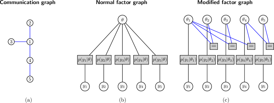
Figure 1: This figure shows how the original factor graph structure of the centralized problem (the left of the factor graphs), with one θ𝜃\theta, is transformed into the factor graph of its corresponding distributed problem (the graph on the right side), as described in Section III-B, with factor vertices as gray boxes and variable vertices as light gray circles. Note that the connections between the equality factors and the θnsubscript𝜃𝑛\theta_{n}’s are decided by the edge set \mathcal{E}. The communication links are highlighted in blue to show how these edges map to edges in the modified factor graph.

When expressing (1) as a factor graph, we obtain a graph with a star topology, irrespective of the network graph. This is shown in Fig. 1: Fig. 1–(a) shows a network graph and Fig. 1–(b) shows the corresponding factor graph. Thus the structure of the factor graph does not match the node graph 𝒢𝒢\mathcal{G}. In order to obtain a factor graph that matches the topology of the graph in Fig. 1–(a), we introduce

f(θ1,,θN)=m=1Np(ym|θm)(m,n)𝕀{θm=θn},𝑓subscript𝜃1subscript𝜃𝑁superscriptsubscriptproduct𝑚1𝑁𝑝conditionalsubscript𝑦𝑚subscript𝜃𝑚subscriptproduct𝑚𝑛subscript𝕀subscript𝜃𝑚subscript𝜃𝑛f(\theta_{1},\dots,\theta_{N})=\prod_{m=1}^{N}p(y_{m}|\theta_{m})\prod_{(m,n)\in\mathcal{E}}\mathbb{I}_{\{\theta_{m}=\theta_{n}\}}, (7)

which is shown in Fig. 1–(c). The marginal of this function with respect to θmsubscript𝜃𝑚\theta_{m} is given by

fm(θm)subscript𝑓𝑚subscript𝜃𝑚\displaystyle f_{m}(\theta_{m}) =θmf(θ1,,θN)=l=1Np(yl|θm),absentsubscriptsimilar-toabsentsubscript𝜃𝑚𝑓subscript𝜃1subscript𝜃𝑁superscriptsubscriptproduct𝑙1𝑁𝑝conditionalsubscript𝑦𝑙subscript𝜃𝑚\displaystyle=\sum_{\sim\theta_{m}}f(\theta_{1},\dots,\theta_{N})=\prod_{l=1}^{N}p(y_{l}|\theta_{m}), (8)

so that for any θ𝜃\theta, fm(θ)=fn(θ)subscript𝑓𝑚𝜃subscript𝑓𝑛𝜃f_{m}(\theta)=f_{n}(\theta), allowing every node to determine the posterior by multiplying fm(θ)subscript𝑓𝑚𝜃f_{m}(\theta) with p(θ)𝑝𝜃p(\theta). The functions fm(θ)subscript𝑓𝑚𝜃f_{m}\left(\theta\right) can be computed using message-passing algorithms, such as BP or URW-BP. The initial belief of node n𝑛n in the log-domain is xn(0)(θ)=logp(yn|θ)superscriptsubscript𝑥𝑛0𝜃𝑝conditionalsubscript𝑦𝑛𝜃x_{n}^{(0)}(\theta)=\log p(y_{n}|\theta). By applying the URW-BP rules in the log-domain, we find (see Appendix A)

xn(1)(θ)superscriptsubscript𝑥𝑛1𝜃\displaystyle x_{n}^{(1)}(\theta) =xn(0)(θ)+ρm𝒩nxm(0)(θ)absentsuperscriptsubscript𝑥𝑛0𝜃𝜌subscript𝑚subscript𝒩𝑛superscriptsubscript𝑥𝑚0𝜃\displaystyle=x_{n}^{(0)}(\theta)+\rho\sum_{m\in\mathcal{N}_{n}}x_{m}^{(0)}(\theta) (9)
xn()(θ)superscriptsubscript𝑥𝑛𝜃\displaystyle x_{n}^{(\ell)}(\theta) =xn(2)(θ)+ρm𝒩n(xm(1)(θ)xn(2)(θ)),absentsuperscriptsubscript𝑥𝑛2𝜃𝜌subscript𝑚subscript𝒩𝑛superscriptsubscript𝑥𝑚1𝜃superscriptsubscript𝑥𝑛2𝜃\displaystyle=x_{n}^{(\ell-2)}(\theta)+\rho\sum_{m\in\mathcal{N}_{n}}(x_{m}^{(\ell-1)}(\theta)-x_{n}^{(\ell-2)}(\theta)), (10)

for >11\ell>1, where ρ(0,1)𝜌01\rho\in(0,1) is the reweighting parameter of URW-BP (where standard BP corresponds to ρ=1𝜌1\rho=1). We call the resulting algorithm uniformly reweighted belief propagation consensus (URW-BPC), due to its linear update resembling a consensus algorithm. Defining the 2N×2N2𝑁2𝑁2N\times 2N URW-BPC matrix

𝑷ρ=[ρ𝑨𝑰Nρ𝑫𝑰N𝑶N],subscript𝑷𝜌delimited-[]𝜌𝑨subscript𝑰𝑁𝜌𝑫subscript𝑰𝑁subscript𝑶𝑁\bm{P}_{\rho}=\left[\begin{array}[]{cc}\rho\bm{A}&\bm{I}_{N}-\rho\bm{D}\\ \bm{I}_{N}&\bm{O}_{N}\end{array}\right], (11)

the update rule in matrix form for URW-BPC for >11\ell>1 is

𝒙()(θ)superscript𝒙𝜃\displaystyle\bm{x}^{(\ell)}(\theta) =[𝑰N𝑶N]𝑷ρ[𝒙(1)(θ)𝒙(2)(θ)]absentdelimited-[]subscript𝑰𝑁subscript𝑶𝑁subscript𝑷𝜌delimited-[]superscript𝒙1𝜃superscript𝒙2𝜃\displaystyle=\left[\begin{array}[]{cc}\bm{I}_{N}&\bm{O}_{N}\end{array}\right]\bm{P}_{\rho}\left[\begin{array}[]{c}\bm{x}^{(\ell-1)}(\theta)\\ \bm{x}^{(\ell-2)}(\theta)\end{array}\right] (15)
=[𝑰N𝑶N]𝑷ρ1[𝒙(1)(θ)𝒙(0)(θ)].absentdelimited-[]subscript𝑰𝑁subscript𝑶𝑁superscriptsubscript𝑷𝜌1delimited-[]superscript𝒙1𝜃superscript𝒙0𝜃\displaystyle=\left[\begin{array}[]{cc}\bm{I}_{N}&\bm{O}_{N}\end{array}\right]\bm{P}_{\mathbf{\rho}}^{\ell-1}\left[\begin{array}[]{c}\bm{x}^{(1)}(\theta)\\ \bm{x}^{(0)}(\theta)\end{array}\right]. (19)

The convergence behavior depends on the power series of the update matrix 𝑷ρsubscript𝑷𝜌\bm{P}_{\rho}.

Remark 1.

We note that, due to (9), it holds that

𝒙()(θ)=[𝑰N𝑶N]𝑷ρ1[ρ𝑨+𝑰N𝑰N]𝒙(0)(θ),superscript𝒙𝜃delimited-[]subscript𝑰𝑁subscript𝑶𝑁superscriptsubscript𝑷𝜌1delimited-[]𝜌𝑨subscript𝑰𝑁subscript𝑰𝑁superscript𝒙0𝜃\bm{x}^{(\ell)}(\theta)=\left[\begin{array}[]{cc}\bm{I}_{N}&\bm{O}_{N}\end{array}\right]\bm{P}_{\rho}^{\ell-1}\left[\begin{array}[]{c}\rho\bm{A}+\bm{I}_{N}\\ \bm{I}_{N}\end{array}\right]\bm{x}^{(0)}(\theta), (20)

which can equivalently be expressed as

𝒙()(θ)=[𝑰N𝑶N]𝑷ρ1(𝑷ρ+𝑰2N)[𝒙(0)(θ)𝟎].superscript𝒙𝜃delimited-[]subscript𝑰𝑁subscript𝑶𝑁superscriptsubscript𝑷𝜌1subscript𝑷𝜌subscript𝑰2𝑁delimited-[]superscript𝒙0𝜃0\bm{x}^{(\ell)}(\theta)=\left[\begin{array}[]{cc}\bm{I}_{N}&\bm{O}_{N}\end{array}\right]\bm{P}_{\rho}^{\ell-1}\left(\bm{P}_{\rho}+\bm{I}_{2N}\right)\left[\begin{array}[]{c}\bm{x}^{(0)}(\theta)\\ \bm{0}\end{array}\right]. (21)

IV General Convergence Results for URW-BPC

Since URW-BPC results in an update rule that can be described in terms of a matrix-vector multiplication, the convergence behavior depends on how the power series 𝑷ρsuperscriptsubscript𝑷𝜌\bm{P}_{\rho}^{\ell} behaves as \ell grows large, which will here be analyzed. First, we establish the fact that λ1=1subscript𝜆11\lambda_{1}=1 is an eigenvalue of any 𝑷ρsubscript𝑷𝜌\bm{P}_{\rho}, and give its corresponding right and left eigenvectors.

Proposition 2.

For any URW-BPC matrix 𝐏ρsubscript𝐏𝜌\bm{P}_{\rho} there is one eigenvalue λ1=1subscript𝜆11\lambda_{1}=1 with geometric multiplicity 111. Its corresponding right and left eigenvectors are 𝐛1=𝟏subscript𝐛11\bm{b}_{1}=\bm{1}, and 𝐜1𝖳=[𝟏𝖳,𝟏𝖳ρ𝟏𝖳𝐃]superscriptsubscript𝐜1𝖳superscript1𝖳superscript1𝖳𝜌superscript1𝖳𝐃\bm{c}_{1}^{\mathsf{T}}=\left[\bm{1}^{\mathsf{T}},\bm{1}^{\mathsf{T}}-\rho\bm{1}^{\mathsf{T}}\bm{D}\right], respectively.

Proof:

See Appendix B-A. ∎

Hence, if all other eigenvalues are strictly less than 1, the convergence of URW-BPC is guaranteed. In contrast to the 𝑾𝑾\bm{W} matrix in belief consensus, the matrix 𝑷ρsubscript𝑷𝜌\bm{P}_{\rho} may not be diagonalizable. Hence, we must consider two cases before providing general convergence conditions.

IV-A Case 1: Diagonalizable 𝐏ρsubscript𝐏𝜌\bm{P}_{\rho}

If 𝑷ρsubscript𝑷𝜌\bm{P}_{\rho} is a diagonalizable matrix, then by eigendecomposition we have that 𝑷ρ=𝑩𝚲𝑩1superscriptsubscript𝑷𝜌𝑩superscript𝚲superscript𝑩1\bm{P}_{\rho}^{\ell}=\bm{B}\bm{\Lambda}^{\ell}\bm{B}^{-1}, where the columns of 𝑩𝑩\bm{B} form an eigenbasis of 𝑷ρsubscript𝑷𝜌\bm{P}_{\rho} and 𝚲𝚲\bm{\Lambda} is a matrix with the eigenvalues of 𝑷ρsubscript𝑷𝜌\bm{P}_{\rho} on the diagonal. Let

𝒛(0)(θ)=[ρ𝑨+𝑰N𝑰N]𝒙(0)(θ),superscript𝒛0𝜃delimited-[]𝜌𝑨subscript𝑰𝑁subscript𝑰𝑁superscript𝒙0𝜃\bm{z}^{(0)}(\theta)=\left[\begin{array}[]{c}\rho\bm{A}+\bm{I}_{N}\\ \bm{I}_{N}\end{array}\right]\bm{x}^{(0)}(\theta), (22)

and express 𝒛(0)(θ)superscript𝒛0𝜃\bm{z}^{(0)}(\theta) in the eigenbasis of 𝑷ρsubscript𝑷𝜌\bm{P}_{\rho} as 𝒛(0)(θ)=𝑩𝜶superscript𝒛0𝜃𝑩𝜶\bm{z}^{(0)}(\theta)=\bm{B}\bm{\alpha}. Now we see that

𝒛()(θ)=𝑷ρ𝒛(0)(θ)=𝑩𝚲𝑩1𝑩𝜶=𝑩𝚲𝜶.superscript𝒛𝜃superscriptsubscript𝑷𝜌superscript𝒛0𝜃𝑩superscript𝚲superscript𝑩1𝑩𝜶𝑩superscript𝚲𝜶\bm{z}^{(\ell)}(\theta)=\bm{P}_{\rho}^{\ell}\bm{z}^{(0)}(\theta)=\bm{B}\bm{\Lambda}^{\ell}\bm{B}^{-1}\bm{B}\bm{\alpha}=\bm{B}\bm{\Lambda}^{\ell}\bm{\alpha}. (23)

We can also express this as

𝒛()(θ)=i=12Nλi𝒃iαi,superscript𝒛𝜃superscriptsubscript𝑖12𝑁superscriptsubscript𝜆𝑖subscript𝒃𝑖subscript𝛼𝑖\bm{z}^{(\ell)}(\theta)=\sum_{i=1}^{2N}\lambda_{i}^{\ell}\bm{b}_{i}\alpha_{i}, (24)

where λisubscript𝜆𝑖\lambda_{i} is the i𝑖ith eigenvalue of 𝑷ρsubscript𝑷𝜌\bm{P}_{\rho}, 𝒃isubscript𝒃𝑖\bm{b}_{i} is the i𝑖ith eigenvector of 𝑷ρsubscript𝑷𝜌\bm{P}_{\rho} (and the i𝑖ith column of 𝑩𝑩\bm{B}), and αisubscript𝛼𝑖\alpha_{i} is the i𝑖ith element of 𝜶𝜶\bm{\alpha}. Since according to Proposition 2, λ1=1subscript𝜆11\lambda_{1}=1, so that

𝒛()(θ)superscript𝒛𝜃\displaystyle\bm{z}^{(\ell)}(\theta) =𝒃1α1+i=22Nλi𝒃iαiabsentsubscript𝒃1subscript𝛼1superscriptsubscript𝑖22𝑁superscriptsubscript𝜆𝑖subscript𝒃𝑖subscript𝛼𝑖\displaystyle=\bm{b}_{1}\alpha_{1}+\sum_{i=2}^{2N}\lambda_{i}^{\ell}\bm{b}_{i}\alpha_{i} (25)
=𝒃1α1+ε.absentsubscript𝒃1subscript𝛼1𝜀\displaystyle=\bm{b}_{1}\alpha_{1}+\varepsilon. (26)

Later, in Proposition 3 we will establish that α1subscript𝛼1\alpha_{1} is the sought value, therefore we consider ε𝜀\varepsilon to be an error term.

IV-B Case 2. Nondiagonalizable 𝐏ρsubscript𝐏𝜌\bm{P}_{\rho}

If 𝑷ρsubscript𝑷𝜌\bm{P}_{\rho} is not diagonalizable, it can be decomposed in its Jordan normal form. Then, 𝑷ρ=𝑩𝑱𝑩1subscript𝑷𝜌𝑩𝑱superscript𝑩1\bm{P}_{\rho}=\bm{B}\bm{J}\bm{B}^{-1}, where the columns of 𝑩𝑩\bm{B} are the generalized eigenvectors of 𝑷ρsubscript𝑷𝜌\bm{P}_{\rho} forming a Jordan basis, and 𝑱𝑱\bm{J} is a Jordan matrix, which is a block diagonal matrix with M<2N𝑀2𝑁M<2N Jordan blocks on its diagonal, i.e.,

𝑱=[𝑱1000000𝑱M].𝑱delimited-[]subscript𝑱1000000subscript𝑱𝑀\bm{J}=\left[\begin{array}[]{ccc}\bm{J}_{1}&0&0\\ 0&\ddots&0\\ 0&0&\bm{J}_{M}\end{array}\right]. (27)

Each Jordan block corresponds to a certain eigenvalue and its generalized eigenvectors. For example, if the eigenvalue λmsubscript𝜆𝑚\lambda_{m} has three generalized eigenvectors, 𝒃m,1subscript𝒃𝑚1\bm{b}_{m,1}, 𝒃m,2subscript𝒃𝑚2\bm{b}_{m,2} and 𝒃m,3subscript𝒃𝑚3\bm{b}_{m,3}, then

𝑱m=[λm100λm100λm].subscript𝑱𝑚delimited-[]subscript𝜆𝑚100subscript𝜆𝑚100subscript𝜆𝑚\bm{J}_{m}=\left[\begin{array}[]{ccc}\lambda_{m}&1&0\\ 0&\lambda_{m}&1\\ 0&0&\lambda_{m}\end{array}\right].

Note that if 𝑷ρsubscript𝑷𝜌\bm{P}_{\rho} is diagonalizable, its Jordan normal form is equal to its eigendecomposition. By expressing 𝒛(0)(θ)=𝑩𝜶superscript𝒛0𝜃𝑩𝜶\bm{z}^{(0)}(\theta)=\bm{B}\bm{\alpha} in the Jordan basis of 𝑷ρsubscript𝑷𝜌\bm{P}_{\rho} and decomposing 𝑷ρsubscript𝑷𝜌\bm{P}_{\rho} in Jordan normal form, we can write

𝒛()(θ)=𝑷ρ𝒛(0)(θ)=𝑩𝑱𝜶,superscript𝒛𝜃superscriptsubscript𝑷𝜌superscript𝒛0𝜃𝑩superscript𝑱𝜶\bm{z}^{(\ell)}(\theta)=\bm{P}_{\rho}^{\ell}\bm{z}^{(0)}(\theta)=\bm{B}\bm{J}^{\ell}\bm{\alpha}, (28)

which we can also express as

𝒛()(θ)=m=1Mj=1rm(i=0min(,rmj)(i)λmi)𝒃m,jαm,j,superscript𝒛𝜃superscriptsubscript𝑚1𝑀superscriptsubscript𝑗1subscript𝑟𝑚superscriptsubscript𝑖0subscript𝑟𝑚𝑗𝑖superscriptsubscript𝜆𝑚𝑖subscript𝒃𝑚𝑗subscript𝛼𝑚𝑗\bm{z}^{(\ell)}(\theta)=\sum_{m=1}^{M}\sum_{j=1}^{r_{m}}\left(\sum_{i=0}^{\min(\ell,r_{m}-j)}\left(\begin{array}[]{c}\ell\\ i\end{array}\right)\lambda_{m}^{\ell-i}\right)\bm{b}_{m,j}\alpha_{m,j}, (29)

where rmsubscript𝑟𝑚r_{m} is the size of the m𝑚mth Jordan block, 𝒃m,jsubscript𝒃𝑚𝑗\bm{b}_{m,j} is the j𝑗jth generalized eigenvector of λmsubscript𝜆𝑚\lambda_{m}, and αm,jsubscript𝛼𝑚𝑗\alpha_{m,j} the corresponding entry in 𝜶𝜶\bm{\alpha}. With λ1=1subscript𝜆11\lambda_{1}=1 and denoting 𝒃1,1α1,1subscript𝒃11subscript𝛼11\bm{b}_{1,1}\alpha_{1,1} by 𝒃1α1subscript𝒃1subscript𝛼1\bm{b}_{1}\alpha_{1}, we can break the sum into three parts

𝒛()(θ)superscript𝒛𝜃\displaystyle\bm{z}^{(\ell)}(\theta) =𝒃1α1+j=2r1i=0min(,r1j)(i)𝒃1,jα1,jabsentsubscript𝒃1subscript𝛼1superscriptsubscript𝑗2subscript𝑟1superscriptsubscript𝑖0subscript𝑟1𝑗𝑖subscript𝒃1𝑗subscript𝛼1𝑗\displaystyle=\bm{b}_{1}\alpha_{1}+\sum_{j=2}^{r_{1}}\sum_{i=0}^{\min(\ell,r_{1}-j)}\left(\begin{array}[]{c}\ell\\ i\end{array}\right)\bm{b}_{1,j}\alpha_{1,j} (32)
+m=2Mj=1rm(i=0min(,rmj)(i)λmi)𝒃m,jαm,jsuperscriptsubscript𝑚2𝑀superscriptsubscript𝑗1subscript𝑟𝑚superscriptsubscript𝑖0subscript𝑟𝑚𝑗𝑖superscriptsubscript𝜆𝑚𝑖subscript𝒃𝑚𝑗subscript𝛼𝑚𝑗\displaystyle+\sum_{m=2}^{M}\sum_{j=1}^{r_{m}}\left(\sum_{i=0}^{\min(\ell,r_{m}-j)}\left(\begin{array}[]{c}\ell\\ i\end{array}\right)\lambda_{m}^{\ell-i}\right)\bm{b}_{m,j}\alpha_{m,j} (35)
=𝒃1α1+ε~+ε.absentsubscript𝒃1subscript𝛼1~𝜀𝜀\displaystyle=\bm{b}_{1}\alpha_{1}+\tilde{\varepsilon}+\varepsilon. (36)

Following the reasoning of the case with a diagonalizable 𝑷ρsubscript𝑷𝜌\bm{P}_{\rho}, any quantity that is not α1subscript𝛼1\alpha_{1} is considered an error term. For the nondiagonalizable case, we split it up into ε𝜀\varepsilon and ε~~𝜀\tilde{\varepsilon}, since these two terms behave fundamentally different with respect to the eigenvalues of 𝑷ρsubscript𝑷𝜌\bm{P}_{\rho}.

IV-C General Convergence Conditions

We are now able to provide insights into α1subscript𝛼1\alpha_{1} as well as the error terms ε~~𝜀\tilde{\varepsilon} and ε𝜀\varepsilon.

Proposition 3.

The quantity α1()=𝐜1𝖳𝐳()(θ)/(𝐜1𝖳𝐛1)superscriptsubscript𝛼1superscriptsubscript𝐜1𝖳superscript𝐳𝜃superscriptsubscript𝐜1𝖳subscript𝐛1\alpha_{1}^{(\ell)}=\bm{c}_{1}^{\mathsf{T}}\bm{z}^{(\ell)}(\theta)/(\bm{c}_{1}^{\mathsf{T}}\bm{b}_{1}) is preserved by the URW-BPC algorithm at each iteration \ell. If URW-BPC converges, then the consensus value is the preserved quantity, and it is equal to

α1=2𝒄1𝖳𝒃1𝟏𝖳𝒙(0)(θ).subscript𝛼12superscriptsubscript𝒄1𝖳subscript𝒃1superscript1𝖳superscript𝒙0𝜃\alpha_{1}=\frac{2}{\bm{c}_{1}^{\mathsf{T}}\bm{b}_{1}}\bm{1}^{\mathsf{T}}\bm{x}^{(0)}\left(\theta\right). (37)
Proof:

See Appendix B-B. ∎

Note according to Proposition 2

𝒄1𝖳𝒃1=2Nρtrace(𝑫).superscriptsubscript𝒄1𝖳subscript𝒃12𝑁𝜌trace𝑫\bm{c}_{1}^{\mathsf{T}}\bm{b}_{1}=2N-\rho\,\mathrm{trace}(\bm{D}). (38)

Hence, what remains is to establish sufficient conditions for URW-BPC to converge and then to establish the corresponding convergence rate. We note the following:

  1. (i)

    When 𝑷ρsubscript𝑷𝜌\bm{P}_{\rho} has an eigenvalue λ=1𝜆1\lambda=-1 with equal geometric and algebraic multiplicities, the corresponding value αisubscript𝛼𝑖\alpha_{i} in (25) or αm,jsubscript𝛼𝑚𝑗\alpha_{m,j} in (29) is zero, since the eigenvector of λ=1𝜆1\lambda=-1 is in the null space of 𝑷ρ+𝑰2Nsubscript𝑷𝜌subscript𝑰2𝑁\bm{P}_{\rho}+\bm{I}_{2N} and is thus canceled out by the initialization (21).

  2. (ii)

    When 𝑷ρsubscript𝑷𝜌\bm{P}_{\rho} is diagonalizable, there is only one eigenvalue λ1=1subscript𝜆11\lambda_{1}=1. If all other eigenvalues are strictly inside the unit circle, or equal to 11-1 with equal geometric and algebraic multiplicities, then ε0𝜀0\varepsilon\to 0 and convergence of URW-BPC (20) is guaranteed to (37) by Proposition 3.

  3. (iii)

    When 𝑷ρsubscript𝑷𝜌\bm{P}_{\rho} is not diagonalizable, if λ1subscript𝜆1\lambda_{1} has a Jordan block of size 1×1111\times 1 and all other eigenvalues are strictly inside the unit circle, or equal to 11-1 with equal geometric and algebraic multiplicities, then ε~=0~𝜀0\tilde{\varepsilon}=0, ε0𝜀0\varepsilon\to 0, and convergence of URW-BPC (20) is guaranteed to (37) by Proposition 3.

Finally, the convergence rate is defined as

r(𝑷ρ)=sup𝒙(0)(θ)c𝟏lim(𝒙()(θ)c𝟏2𝒙(0)(θ)c𝟏2)1/,𝑟subscript𝑷𝜌subscriptsupremumsuperscript𝒙0𝜃𝑐1subscriptsuperscriptsubscriptnormsuperscript𝒙𝜃𝑐12subscriptnormsuperscript𝒙0𝜃𝑐121r\left(\bm{P}_{\rho}\right)=\sup_{\bm{x}^{(0)}(\theta)\neq c\bm{1}}\lim_{\ell\to\infty}\left(\frac{\left\|\bm{x}^{(\ell)}(\theta)-c\bm{1}\right\|_{2}}{\left\|\bm{x}^{(0)}(\theta)-c\bm{1}\right\|_{2}}\right)^{1/\ell}, (39)

provided that the algorithm is convergent, and at least one eigenvalue strictly inside the unit circle is nonzero. For such cases, we consider the eigenvalues of 𝑷ρsubscript𝑷𝜌\bm{P}_{\rho} to be sorted such that |λ1||λ2||λ2N|subscript𝜆1subscript𝜆2subscript𝜆2𝑁\left|\lambda_{1}\right|\geq\left|\lambda_{2}\right|\geq\dots\geq\left|\lambda_{2N}\right|. The convergence rate is determined by |λ~|~𝜆|\tilde{\lambda}| where λ~=maxi|λi|~𝜆subscript𝑖subscript𝜆𝑖\tilde{\lambda}=\max_{i}|\lambda_{i}| for i𝑖i such that |λi|<1subscript𝜆𝑖1|\lambda_{i}|<1, such that a smaller |λ~|~𝜆|\tilde{\lambda}| gives a faster convergence.

V Convergence on Specific Graph Types

In this section, we analyze the convergence properties of URW-BPC for three specific types of graphs. We first consider tree-graphs, recovering the well-known finite-time BP convergence result via the formulation (21). Then, we consider the regular graphs, for which BP is generally not guaranteed to converge. Finally, we consider general connected graphs, for which we can build on the results from regular graphs.

V-A Tree Graphs

For trees, the following proposition establishes the possible eigenvalues of 𝑷1subscript𝑷1\bm{P}_{1}.

Proposition 4.

The URW-BPC matrix 𝐏1subscript𝐏1\bm{P}_{1} of any tree-graph has three distinct eigenvalues: λ1=1subscript𝜆11\lambda_{1}=1, λ2=1subscript𝜆21\lambda_{2}=-1, and λi=0subscript𝜆𝑖0\lambda_{i}=0 for i=3,,2N𝑖32𝑁i=3,\dots,2N.

Proof:

See Appendix B-C. ∎

We then immediately find the following well-known results for trees, that BP converges in a finite number of iterations.

Theorem 5.

If 𝒢𝒢\mathcal{G} is a tree graph of N𝑁N nodes, then URW-BPC with 𝐏1subscript𝐏1\bm{P}_{1} converges to consensus after at most 2N32𝑁32N-3 iterations. Moreover, with the initialization as in (20), the consensus value after κ𝜅\kappa iterations (κ𝜅\kappa such that consensus is reached) is

𝒙(κ)(θ)=m=1Nxm(0)(θ)𝟏.superscript𝒙𝜅𝜃superscriptsubscript𝑚1𝑁superscriptsubscript𝑥𝑚0𝜃1\bm{x}^{(\kappa)}(\theta)=\sum_{m=1}^{N}x_{m}^{(0)}(\theta)\bm{1}. (40)
Proof:

Due to Proposition 4, 𝑷1subscript𝑷1\bm{P}_{1} has 2N22𝑁22N-2 eigenvalues λ=0𝜆0\lambda=0. Hence, the largest possible size of its corresponding Jordan block, denoted by 𝑱0subscript𝑱0\bm{J}_{0}, is 2N22𝑁22N-2. Since 𝑱02N2=𝑶superscriptsubscript𝑱02𝑁2𝑶\bm{J}_{0}^{2N-2}=\bm{O}, the error contribution from the eigenvalues equal to zero is zero after at most 2N32𝑁32N-3 iterations. Furthermore, applying the results from Propositions 2 and 3, and using the fact that the sum of the degrees trace(𝑫)=2N2trace𝑫2𝑁2\mathrm{trace}(\bm{D})=2N-2 for undirected tree-graphs in (38), the consensus value α1subscript𝛼1\alpha_{1} is given by (40). ∎

V-B Regular Graphs

In order to understand when URW-BPC converges, we first show how to choose the weighting parameter ρ𝜌\rho in order to guarantee convergence. Then we proceed to optimize ρ𝜌\rho for a given graph 𝒢𝒢\mathcal{G} such that the magnitude of the largest eigenvalue inside the unit circle, |λ~|~𝜆|\tilde{\lambda}|, is minimized. We recall that for k𝑘k-regular graphs, the largest eigenvalue of the adjacency matrix is μ1=ksubscript𝜇1𝑘\mu_{1}=k for non-bipartite graphs, while for bipartite graphs, eigenvalues come in symmetric pairs, so that both μ1=ksubscript𝜇1𝑘\mu_{1}=k and μ2=ksubscript𝜇2𝑘\mu_{2}=-k are eigenvalues [25, Prop.2.3].

V-B1 Convergence

To find for which ρ𝜌\rho URW-BPC converges on k𝑘k-regular graphs, we first show how the eigenvalues of 𝑷ρsubscript𝑷𝜌\bm{P}_{\rho} and 𝑨𝑨\bm{A} are connected in terms of magnitudes. Note, that the eigenvalues of 𝑷ρsubscript𝑷𝜌\bm{P}_{\rho} and 𝑨𝑨\bm{A} are sorted such that |λ1||λ2||λ2N|subscript𝜆1subscript𝜆2subscript𝜆2𝑁|\lambda_{1}|\geq|\lambda_{2}|\geq\dots\geq|\lambda_{2N}| and |μ1||μ2||μN|subscript𝜇1subscript𝜇2subscript𝜇𝑁|\mu_{1}|\geq|\mu_{2}|\geq\dots\geq|\mu_{N}|.

Lemma 6.

Let ρ(0,1]𝜌01\rho\in(0,1]. Then the eigenvalue λisubscript𝜆𝑖\lambda_{i} of 𝐏ρsubscript𝐏𝜌\bm{P}_{\rho}, λi0subscript𝜆𝑖0\lambda_{i}\neq 0, can be expressed in terms of μisubscript𝜇𝑖\mu_{i}, and its magnitude is

|λi|=12|μiρ+μi2ρ24kρ+4|.subscript𝜆𝑖12subscript𝜇𝑖𝜌superscriptsubscript𝜇𝑖2superscript𝜌24𝑘𝜌4\left|\lambda_{i}\right|=\frac{1}{2}\left|\mu_{i}\rho+\sqrt{\mu_{i}^{2}\rho^{2}-4k\rho+4}\right|. (41)
Proof:

See Appendix C-A. ∎

Note that for λi=0subscript𝜆𝑖0\lambda_{i}=0 with eigenvector [𝒗𝖳,𝒘𝖳]𝖳superscriptsuperscript𝒗𝖳superscript𝒘𝖳𝖳[\bm{v}^{\mathsf{T}},\bm{w}^{\mathsf{T}}]^{\mathsf{T}}, we have that

ρ𝑨𝒗+𝒘ρ𝑫𝒘𝜌𝑨𝒗𝒘𝜌𝑫𝒘\displaystyle\rho\bm{A}\bm{v}+\bm{w}-\rho\bm{D}\bm{w} =0absent0\displaystyle=0 (42)
𝒗𝒗\displaystyle\bm{v} =0.absent0\displaystyle=0. (43)

We conclude that for λi=0subscript𝜆𝑖0\lambda_{i}=0, we must have that kρ=1𝑘𝜌1k\rho=1. Note however, that this does not mean that all eigenvalues are equal to 0 for ρ=1/k𝜌1𝑘\rho=1/k.

Now, since μ1=ksubscript𝜇1𝑘\mu_{1}=k, the magnitude of λ1subscript𝜆1\lambda_{1} of 𝑷ρsubscript𝑷𝜌\bm{P}_{\rho} is either 111 or |ρk1|𝜌𝑘1\left|\rho k-1\right|. Thus, we can prove the following result regarding the convergence conditions of URW-BPC.

Theorem 7.

For any k𝑘k-regular graph, URW-BPC is convergent if and only if ρ(0,2/k)𝜌02𝑘\rho\in(0,2/k), and the asymptotic consensus value is

lim𝒙()(θ)=1N(1ρk/2)m=1Nxm(0)(θ)𝟏.subscriptsuperscript𝒙𝜃1𝑁1𝜌𝑘2superscriptsubscript𝑚1𝑁superscriptsubscript𝑥𝑚0𝜃1\lim_{\ell\to\infty}\bm{x}^{(\ell)}\left(\theta\right)=\frac{1}{N(1-\rho k/2)}\sum_{m=1}^{N}x_{m}^{(0)}\left(\theta\right)\bm{1}. (44)
Proof:

See Appendix C-B. ∎

This result provides the interval for ρ𝜌\rho within which we can guarantee convergence, and to which value the algorithm converges.

V-B2 Optimizing the Convergence Rate

In order to maximize convergence rate, we show which ρ𝜌\rho minimizes the largest eigenvalue within the unit circle, denoted by |λ~|<1~𝜆1|\tilde{\lambda}|<1.

Theorem 8.

The choice of ρ𝜌\rho that minimizes |λ~|~𝜆|\tilde{\lambda}| is

ρopt=2μ~2(kk2μ~2),\rho_{\mathrm{opt}}=\frac{2}{\tilde{\mu}{}^{2}}\left(k-\sqrt{k^{2}-\tilde{\mu}^{2}}\right), (45)

where μ~=maxi|μi|~𝜇subscript𝑖subscript𝜇𝑖\tilde{\mu}=\max_{i}\left|\mu_{i}\right| for i𝑖i such that |μi|<ksubscript𝜇𝑖𝑘\left|\mu_{i}\right|<k. The magnitude of the second largest eigenvalue of 𝐏ρoptsubscript𝐏subscript𝜌opt\bm{P}_{\rho_{\mathrm{opt}}} is

|λ~|~𝜆\displaystyle|\tilde{\lambda}| =|1μ~(kk2μ~2)|.absent1~𝜇𝑘superscript𝑘2superscript~𝜇2\displaystyle=\left|\frac{1}{\tilde{\mu}}\left(k-\sqrt{k^{2}-\tilde{\mu}^{2}}\right)\right|. (46)
Proof:

See Appendix C-C. ∎

Remark 9.

For any k𝑘k-regular non-bipartite graph 𝒢𝒢\mathcal{G}, μ~=μ2~𝜇subscript𝜇2\tilde{\mu}=\mu_{2}. However, for a k𝑘k-regular bipartite graph we have that μ2=μ1=ksubscript𝜇2subscript𝜇1𝑘\mu_{\mathrm{2}}=-\mu_{1}=-k. Hence, choosing ρoptsubscript𝜌opt\rho_{\mathrm{opt}} with μ2subscript𝜇2\mu_{2} instead of μ~~𝜇\tilde{\mu} in this case would yield ρopt=2/ksubscript𝜌opt2𝑘\rho_{\mathrm{opt}}=2/k, which in turn gives (see (41)), |λi|2=1/k2|μ±μ2k2|2=1superscriptsubscript𝜆𝑖21superscript𝑘2superscriptplus-or-minus𝜇superscript𝜇2superscript𝑘221\left|\lambda_{i}\right|^{2}=1/k^{2}\left|\mu\pm\sqrt{\mu^{2}-k^{2}}\right|^{2}=1, for every eigenvalue λisubscript𝜆𝑖\lambda_{i} of 𝑷ρsubscript𝑷𝜌\bm{P}_{\rho}. Hence, the optimal reweighting for k𝑘k-regular bipartite graphs is achieved with μ~=μ3~𝜇subscript𝜇3\tilde{\mu}=\mu_{3}. Another consequence of μ2=ksubscript𝜇2𝑘\mu_{2}=-k is that there is always an eigenvalue λ=1𝜆1\lambda=-1 for bipartite graphs. This remark also applies to tree-graphs, which is a class of bipartite graphs, where 𝑷1subscript𝑷1\bm{P}_{1} of a tree-graph has an eigenvalue λ=1𝜆1\lambda=-1. However, the component associated with this eigenvalue is irrelevant, as it is removed by the initialization procedure. This relies on the following result.

Proposition 10.

For a URW-BPC matrix 𝐏ρsubscript𝐏𝜌\bm{P}_{\rho}, the algebraic and geometric multiplicites of λ=±1𝜆plus-or-minus1\lambda=\pm 1 are equal.

Proof:

See Appendix C-D.

V-B3 Limit Results for k𝑘k-regular Graphs

Due to their structure, the eigenvalue distribution of 𝑨𝑨\bm{A} for large k𝑘k-regular graphs is given by [26] (with 𝒢𝒢\mathcal{G} satisfying certain properties regarding the number of cycles in the graph, for details see [26])

f(μ)={k(4(k1)μ2)1/22π(k2μ2),|μ|2k10,|μ|>2k1.𝑓𝜇cases𝑘superscript4𝑘1superscript𝜇2122𝜋superscript𝑘2superscript𝜇2𝜇2𝑘10𝜇2𝑘1f(\mu)=\begin{cases}\frac{k\left(4\left(k-1\right)-\mu^{2}\right)^{1/2}}{2\pi\left(k^{2}-\mu^{2}\right)},&\left|\mu\right|\leq 2\sqrt{k-1}\\ 0,&\left|\mu\right|>2\sqrt{k-1}.\end{cases} (47)

This means that limN|μ2|=2k1subscript𝑁subscript𝜇22𝑘1\lim_{N\to\infty}\left|\mu_{2}\right|=2\sqrt{k-1}, and thus

limNρopt=12(k1)(kk24(k1)),subscript𝑁subscript𝜌opt12𝑘1𝑘superscript𝑘24𝑘1\lim_{N\to\infty}\rho_{\mathrm{opt}}=\frac{1}{2(k-1)}\left(k-\sqrt{k^{2}-4(k-1)}\right), (48)

so that the second largest eigenvalue of 𝑷ρsubscript𝑷𝜌\bm{P}_{\rho} for non-bipartite graphs tends to

limN|λ2,BPC|=12k1(kk24(k1)).subscript𝑁subscript𝜆2BPC12𝑘1𝑘superscript𝑘24𝑘1\lim_{N\to\infty}\left|\lambda_{2,\mathrm{BPC}}\right|=\frac{1}{2\sqrt{k-1}}\left(k-\sqrt{k^{2}-4\left(k-1\right)}\right). (49)

For the belief consensus, |λ2,Metr|subscript𝜆2Metr\left|\lambda_{2,\mathrm{Metr}}\right| of 𝑾=𝑰Nξ𝑳𝑾subscript𝑰𝑁𝜉𝑳\bm{W}=\bm{I}_{N}-\xi\bm{L} tends to

limN|λ2,Metr|=1+2k1k+1>limN|λ2,BPC|,subscript𝑁subscript𝜆2Metr12𝑘1𝑘1subscript𝑁subscript𝜆2BPC\lim_{N\to\infty}\left|\lambda_{2,\mathrm{Metr}}\right|=\frac{1+2\sqrt{k-1}}{k+1}>\lim_{N\to\infty}\left|\lambda_{2,\mathrm{BPC}}\right|, (50)

so that BPC always converges faster than belief consensus on large k𝑘k-regular graph.

V-C General Graphs

For general graphs, it is not obvious how to render BPC convergent. A possible approach is to determine a spanning tree of the network graph and then running BPC with finite-time convergence [27]. However, we can also build on the results from regular graphs. We outline two procedures to convert a general graph to a regular graph.

  1. (i)

    Edge addition: The simplest way to make a graph into a k𝑘k-regular graph, is to first determine the maximum node degree dmaxsubscript𝑑maxd_{\mathrm{max}} (this can be done through max-consensus). Then a node i𝑖i with degree disubscript𝑑𝑖d_{i} adds dmaxdisubscript𝑑maxsubscript𝑑𝑖d_{\mathrm{max}}-d_{i} self-loops. Then BPC with ρoptsubscript𝜌opt\rho_{\mathrm{opt}} set based on k=dmax𝑘subscript𝑑maxk=d_{\mathrm{max}} and μ~~𝜇\tilde{\mu} of the new 𝑨𝑨\bm{A}, is applied.

  2. (ii)

    Edge deletion: A more complex way to create a k𝑘k-regular graph is by selectively deleting edges from those nodes with maximum degree, while maintaining connectivity. This procedure can be applied until a certain minimal value for dmaxsubscript𝑑maxd_{\mathrm{max}} is attained.

VI Numerical Results and Discussion

VI-A Simulation Parameters

We present numerical results comparing the URW-BPC algorithms with Metropolis weighted belief consensus. The simulations were performed with the number of nodes N=100𝑁100N=100, with a fixed 𝒢𝒢\mathcal{G} for tree-graphs and random 𝒢𝒢\mathcal{G} for k𝑘k-regular graphs. The node degree for the k𝑘k-regular graphs was fixed to k=4𝑘4k=4. The elements of the initial data 𝒙(0)(θ)superscript𝒙0𝜃\bm{x}^{(0)}(\theta) were generated according to a standard normal distribution. We calculated the averaged (over instances of 𝒙(0)(θ)superscript𝒙0𝜃\bm{x}^{(0)}(\theta) for tree-graphs, and over both 𝒙(0)(θ)superscript𝒙0𝜃\bm{x}^{(0)}(\theta) and 𝒢𝒢\mathcal{G} for k𝑘k-regular graphs) and normalized mean squared error (MSE), with the MSE being normalized with respect to the initial consensus error. The simulations were performed over 100 Monte Carlo runs.

VI-B Results for Tree-graphs
Refer to caption
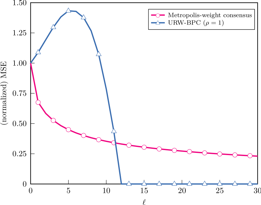
Figure 2: The normalized MSE of URW-BPC vs. BC with Metropolis-type weights over a random tree-graph, with diameter 121212 and N=100𝑁100N=100. The error is averaged over 100100100 instances of random initial data 𝒙(0)(θ)superscript𝒙0𝜃\bm{x}^{(0)}(\theta), but with a fixed graph 𝒢𝒢\mathcal{G}.

The simulated error of URW-BPC on a tree-graph is shown in Fig. 2. We observe that the algorithm indeed reaches consensus in a finite number of steps. However, before reaching consensus, the error of URW-BPC behaves differently from that of the other consensus algorithm. The increasing error we see can be explained by ε1subscript𝜀1\varepsilon_{1} in (36). It takes a few iterations for the Jordan blocks of the eigenvalues λi=0subscript𝜆𝑖0\lambda_{i}=0 to become zero, and until they do, the error they contribute with increases as k𝑘k increases.

VI-C Results for k𝑘k-regular Graphs

Refer to caption
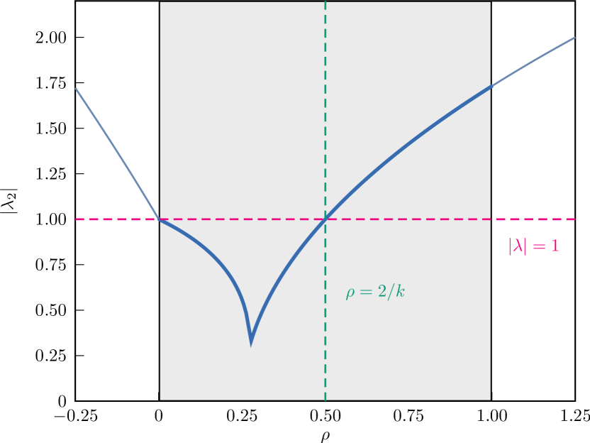
Figure 3: The magnitude of the eigenvalue λ2subscript𝜆2\lambda_{2} of 𝑷ρsubscript𝑷𝜌\bm{P}_{\rho} generated from the eigenvalue μ2subscript𝜇2\mu_{2} of 𝑨𝑨\bm{A} plotted as a function of the weighting parameter ρ𝜌\rho, for the k𝑘k-regular small-world graph with k=4𝑘4k=4 and N=10𝑁10N=10 described in the example in Section VI-C.
Refer to caption
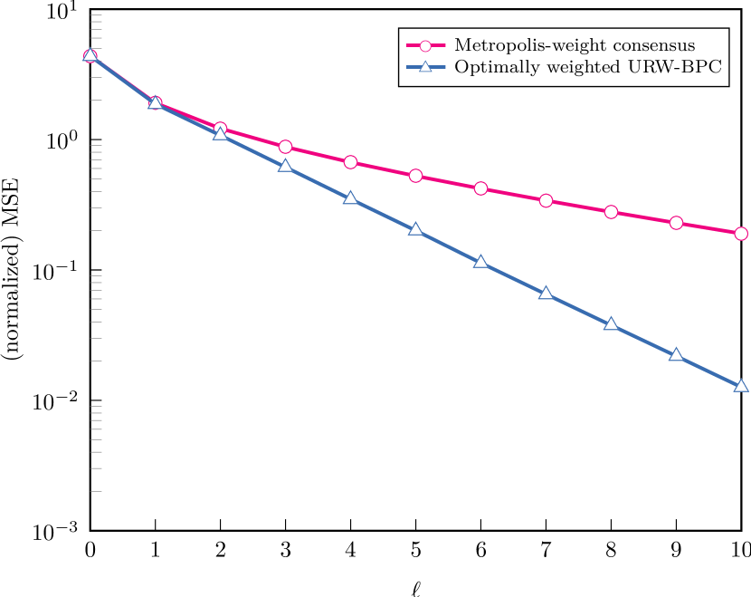
Figure 4: The normalized MSE of URW-BPC with ρ=ρopt𝜌subscript𝜌opt\rho=\rho_{\mathrm{opt}} vs. BC with Metropolis-type weights over random regular graphs with N=100𝑁100N=100 and k=4𝑘4k=4, plotted in log scale as a function of iterations. The error is averaged over 100100100 instances of random initial data 𝒙(0)(θ)superscript𝒙0𝜃\bm{x}^{(0)}(\theta), and graphs 𝒢𝒢\mathcal{G}.
Refer to caption
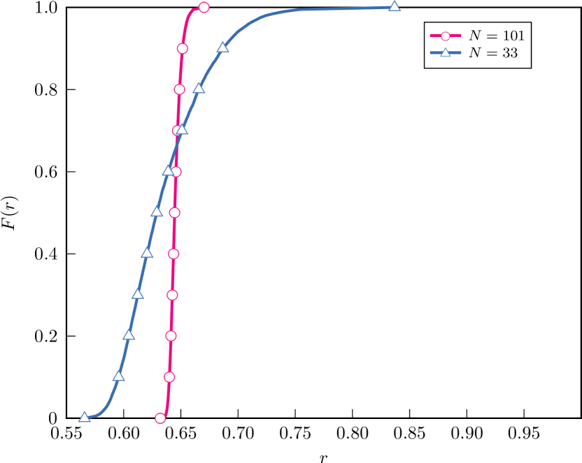
Figure 5: Empirical cdf’s of r=|λ2,BPC|/|λ2,Metr|𝑟subscript𝜆2BPCsubscript𝜆2Metrr=\left|\lambda_{2,\mathrm{BPC}}\right|/\left|\lambda_{2,\mathrm{Metr}}\right| for two types of k𝑘k-regular graphs with N=101𝑁101N=101 (red) and N=33𝑁33N=33 (blue), and k=4𝑘4k=4. The empirical cdf is from 100010001000 instances of random graphs.

To illustrate the benefit of URW-BPC on k𝑘k-regular graphs, we provide the following example of URW-BPC on a so called small-world graph [28]. Let 𝒢𝒢\mathcal{G} be of the type detailed in [28, Appendix A]. For this type of graph, there exist closed-form expressions for the eigenvalues of 𝑨𝑨\bm{A}. In particular, if we let 𝒢𝒢\mathcal{G} be such a graph with N=10𝑁10N=10 and k=4𝑘4k=4, we have that μ22.23subscript𝜇22.23\mu_{2}\approx 2.23. Hence, using (45) to calculate the optimal ρ𝜌\rho, we get from (46) that |λ2|0.31subscript𝜆20.31\left|\lambda_{2}\right|\approx 0.31. On the other hand, using BC on this graph with step-size ε=0.25𝜀0.25\varepsilon=0.25 yields |λ2|0.56subscript𝜆20.56\left|\lambda_{2}\right|\approx 0.56.

In Fig. 4 we show how the average error of optimally weighted URW-BPC and belief consensus compare. The error is averaged over instances of the graph 𝒢𝒢\mathcal{G} as well as the initial data 𝒙(0)(θ)superscript𝒙0𝜃\bm{x}^{(0)}(\theta). Clearly, URW-BPC outperforms belief consensus in terms of convergence rate.

In Fig. 5 we compare the magnitude of λ2subscript𝜆2\lambda_{2} for the two consensus algorithms by taking the ratio r=|λ2,BPC|/|λ2,Metr|𝑟subscript𝜆2BPCsubscript𝜆2Metrr=\left|\lambda_{2,\mathrm{BPC}}\right|/\left|\lambda_{2,\mathrm{Metr}}\right|, plotting the empirical cumulative distribution function (cdf) over 10,000 Monte Carlo runs. Clearly, URW-BPC always outperforms belief consensus, since the ratio stays well below one. Moreover, as we increase the network size, we see that the ratio converges to the specific limit value discussed in Section V-B3.

VI-D Results for a General Graph
Refer to caption
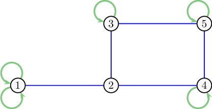
Figure 6: Example of nonregular graph made k𝑘k-regular by adding self loops. In this case k=3𝑘3k=3. The original communication graph is indicated by the blue edges, while the added self-loops are indicated in green.
Refer to caption
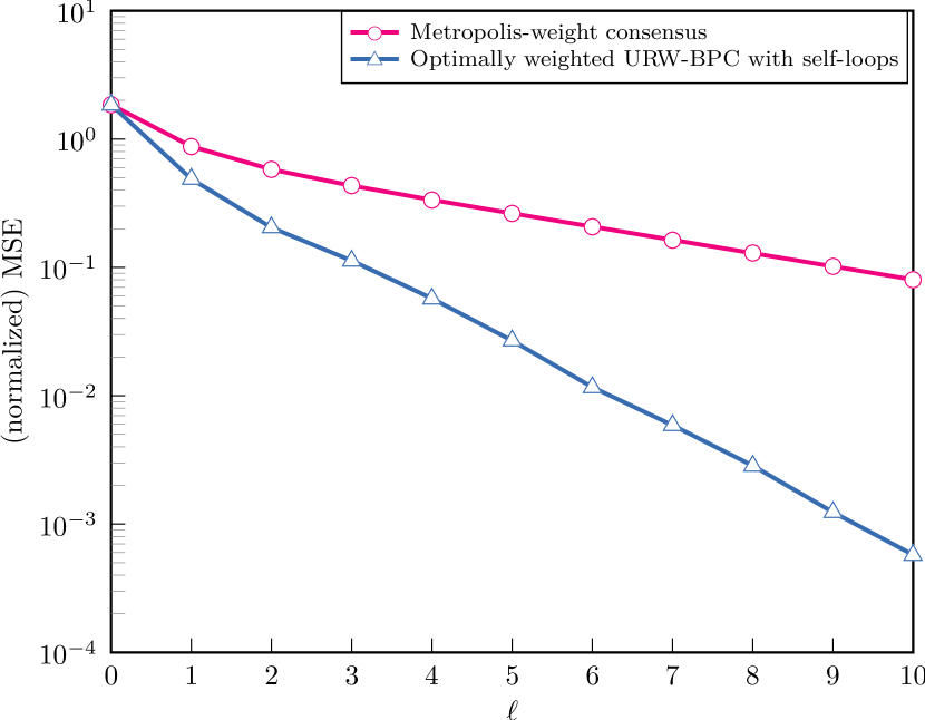
Figure 7: The normalized MSE of URW-BPC with ρ=ρopt𝜌subscript𝜌opt\rho=\rho_{\mathrm{opt}} with added self-loops to make the graph k𝑘k-regular vs. BC with Metropolis-type weights, with N=100𝑁100N=100 and k=3𝑘3k=3, plotted in log scale as a function of iterations. The error is averaged over 100100100 instances of random initial data 𝒙(0)(θ)superscript𝒙0𝜃\bm{x}^{(0)}(\theta).

To illustrate the method for general graphs discussed in Section V-C, we perform numerical simulations for the graph shown in Fig. 6, both without self-loops and Metropolis weight consensus, and with added self-loops and optimally weighted (according to the result of Theorem 8) URW-BPC. The results are shown in Fig. 7. We see that the strategy of adding self-loops and running URW-BPC on the resulting k=3𝑘3k=3 regular graph indeed works well, and asymptotically outperforms belief consensus on the original graph.

VII Conclusion

We studied the uniformly reweighted belief propagation algorithm for distributed likelihood fusion, which was described by a factor graph with strong interactions, generally considered a challenging case for belief propagation. The belief propagation consensus algorithm resulted in a linear update rule much like a consensus algorithm with memory. By eigenvalue analysis we were able to prove a collection of results on several types of graphs: (i) we recovered the classical finite-time convergence of belief propagation on tree graphs for the likelihood fusion problem; (ii) we provided conditions on the reweighting parameter necessary and sufficient for convergence, and (iii) we found an analytical expression for the reweighting parameter optimizing convergence rate, on k𝑘k-regular graphs, and on general graphs artificially transformed into k𝑘k-regular graphs by adding self-loops or removing edges. Based on both numerical results, and eigenvalue limits on large k𝑘k-regular graphs, belief propagation consensus outperformed consensus with Metropolis-type weights. Open issues include analytically comparing the performance of belief propagation consensus to other algorithms for distributed likelihood fusion, and to investigate how it compares to consensus algorithms with memory.

Appendix A Derivation of the URW-BPC algorithm

According to the message-passing equations of the uniformly reweighted BP [19], we can write the marginal belief of some variable θnsubscript𝜃𝑛\theta_{n} of node n𝑛n at iteration \ell as

bn()(θn)p(yn|θn)m𝒩n(μmn()(θn))ρ,proportional-tosuperscriptsubscript𝑏𝑛subscript𝜃𝑛𝑝conditionalsubscript𝑦𝑛subscript𝜃𝑛subscriptproduct𝑚subscript𝒩𝑛superscriptsuperscriptsubscript𝜇𝑚𝑛subscript𝜃𝑛𝜌b_{n}^{(\ell)}(\theta_{n})\propto p(y_{n}|\theta_{n})\prod_{m\in\mathcal{N}_{n}}\left(\mu_{m\rightarrow n}^{(\ell)}(\theta_{n})\right)^{\rho}, (51)

for ρ(0,1]𝜌01\rho\in(0,1], where the message from node m𝑚m to node n𝑛n at iteration \ell is computed by

μmn()(θn)superscriptsubscript𝜇𝑚𝑛subscript𝜃𝑛\displaystyle\mu_{m\rightarrow n}^{(\ell)}(\theta_{n}) θm𝕀{θm=θn}p(ym|θm)u𝒩m\n(μum(1)(θm))ρ(μnm(1)(θm))1ρproportional-toabsentsubscriptsubscript𝜃𝑚subscript𝕀subscript𝜃𝑚subscript𝜃𝑛𝑝conditionalsubscript𝑦𝑚subscript𝜃𝑚subscriptproduct𝑢\subscript𝒩𝑚𝑛superscriptsuperscriptsubscript𝜇𝑢𝑚1subscript𝜃𝑚𝜌superscriptsuperscriptsubscript𝜇𝑛𝑚1subscript𝜃𝑚1𝜌\displaystyle\propto\sum_{\theta_{m}}\mathbb{I}_{\{\theta_{m}=\theta_{n}\}}p(y_{m}|\theta_{m})\frac{\prod_{u\in\mathcal{N}_{m}\backslash n}\left(\mu_{u\rightarrow m}^{(\ell-1)}(\theta_{m})\right)^{\rho}}{\left(\mu_{n\rightarrow m}^{(\ell-1)}(\theta_{m})\right)^{1-\rho}} (52)
=θm𝕀{θm=θn}bm(1)(θm)(μnm(1)(θm))1ρ(μnm(1)(θm))ρabsentsubscriptsubscript𝜃𝑚subscript𝕀subscript𝜃𝑚subscript𝜃𝑛superscriptsubscript𝑏𝑚1subscript𝜃𝑚superscriptsuperscriptsubscript𝜇𝑛𝑚1subscript𝜃𝑚1𝜌superscriptsuperscriptsubscript𝜇𝑛𝑚1subscript𝜃𝑚𝜌\displaystyle=\sum_{\theta_{m}}\mathbb{I}_{\{\theta_{m}=\theta_{n}\}}\frac{b_{m}^{(\ell-1)}(\theta_{m})}{\left(\mu_{n\rightarrow m}^{(\ell-1)}(\theta_{m})\right)^{1-\rho}\left(\mu_{n\rightarrow m}^{(\ell-1)}(\theta_{m})\right)^{\rho}} (53)
=bm(1)(θn)μnm(1)(θn).absentsuperscriptsubscript𝑏𝑚1subscript𝜃𝑛superscriptsubscript𝜇𝑛𝑚1subscript𝜃𝑛\displaystyle=\frac{b_{m}^{(\ell-1)}(\theta_{n})}{\mu_{n\rightarrow m}^{(\ell-1)}(\theta_{n})}. (54)

We note that θn=θm=θsubscript𝜃𝑛subscript𝜃𝑚𝜃\theta_{n}=\theta_{m}=\theta, and plug (54) into (51)

bn()(θ)superscriptsubscript𝑏𝑛𝜃\displaystyle b_{n}^{(\ell)}(\theta) p(yn|θ)m𝒩n(bm(1)(θ)μnm(1)(θ))ρproportional-toabsent𝑝conditionalsubscript𝑦𝑛𝜃subscriptproduct𝑚subscript𝒩𝑛superscriptsuperscriptsubscript𝑏𝑚1𝜃superscriptsubscript𝜇𝑛𝑚1𝜃𝜌\displaystyle\propto p(y_{n}|\theta)\prod_{m\in\mathcal{N}_{n}}\left(\frac{b_{m}^{(\ell-1)}(\theta)}{\mu_{n\rightarrow m}^{(\ell-1)}(\theta)}\right)^{\rho} (55)
=p(yn|θ)m𝒩n(bm(1)(θ)bn(2)(θ)μmn(2)(θ))ρabsent𝑝conditionalsubscript𝑦𝑛𝜃subscriptproduct𝑚subscript𝒩𝑛superscriptsuperscriptsubscript𝑏𝑚1𝜃superscriptsubscript𝑏𝑛2𝜃superscriptsubscript𝜇𝑚𝑛2𝜃𝜌\displaystyle=p(y_{n}|\theta)\prod_{m\in\mathcal{N}_{n}}\left(\frac{b_{m}^{(\ell-1)}(\theta)}{b_{n}^{(\ell-2)}(\theta)}\mu_{m\rightarrow n}^{(\ell-2)}(\theta)\right)^{\rho} (56)
=bn(2)(θ)m𝒩n(bm(1)(θ)bn(2)(θ))ρ.absentsuperscriptsubscript𝑏𝑛2𝜃subscriptproduct𝑚subscript𝒩𝑛superscriptsuperscriptsubscript𝑏𝑚1𝜃superscriptsubscript𝑏𝑛2𝜃𝜌\displaystyle=b_{n}^{(\ell-2)}(\theta)\prod_{m\in\mathcal{N}_{n}}\left(\frac{b_{m}^{(\ell-1)}(\theta)}{b_{n}^{(\ell-2)}(\theta)}\right)^{\rho}. (57)

For the initial values of the marginals, we assume that μmn(0)(θ)=1superscriptsubscript𝜇𝑚𝑛0𝜃1\mu_{m\rightarrow n}^{(0)}(\theta)=1 for all nodes n𝑛n, all m𝒩n𝑚subscript𝒩𝑛m\in\mathcal{N}_{n}. Hence, by (51) we have that bn(0)(θ)=p(yn|θ)superscriptsubscript𝑏𝑛0𝜃𝑝conditionalsubscript𝑦𝑛𝜃b_{n}^{(0)}(\theta)=p(y_{n}|\theta). Now we can compute the marginals at iteration =11\ell=1 by using (55), which gives bn(2)(θ)=p(yn|θ)m𝒩n(p(ym|θ))ρsuperscriptsubscript𝑏𝑛2𝜃𝑝conditionalsubscript𝑦𝑛𝜃subscriptproduct𝑚subscript𝒩𝑛superscript𝑝conditionalsubscript𝑦𝑚𝜃𝜌b_{n}^{(2)}(\theta)=p(y_{n}|\theta)\prod_{m\in\mathcal{N}_{n}}\left(p(y_{m}|\theta)\right)^{\rho}.

Appendix B Proofs of Propositions

B-A Proof of Proposition 2

Proof:

Let 𝒃1=[𝒗𝖳,𝒘𝖳]𝖳subscript𝒃1superscriptsuperscript𝒗𝖳superscript𝒘𝖳𝖳\bm{b}_{1}=[\bm{v}^{\mathsf{T}},\bm{w}^{\mathsf{T}}]^{\mathsf{T}} be a right eigenvector corresponding to the eigenvalue λ1=1subscript𝜆11\lambda_{1}=1. Then, it holds that

𝒗𝒗\displaystyle\bm{v} =ρ𝑨𝒗+(𝑰Nρ𝑫)𝒘absent𝜌𝑨𝒗subscript𝑰𝑁𝜌𝑫𝒘\displaystyle=\rho\bm{A}\bm{v}+(\bm{I}_{N}-\rho\bm{D})\bm{w} (58)
𝒘𝒘\displaystyle\bm{w} =𝒗,absent𝒗\displaystyle=\bm{v}, (59)

which boils down to 𝑳𝒗=𝟎𝑳𝒗0\bm{L}\bm{v}=\bm{0}, where 𝑳=𝑫𝑨𝑳𝑫𝑨\bm{L}=\bm{D}-\bm{A} is the graph Laplacian. The graph Laplacian 𝑳𝑳\bm{L} of a connected graph has an eigenvalue ν=0𝜈0\nu=0 with algebraic multiplicity equal to 1, and its right eigenvector is 𝒗=𝟏𝒗1\bm{v}=\bm{1}. Thus, λ1=1subscript𝜆11\lambda_{1}=1 has geometric multiplicity equal to 1. Since (59) states that 𝒘=𝒗𝒘𝒗\bm{w}=\bm{v}, we see that 𝒃1=𝟏subscript𝒃11\bm{b}_{1}=\bm{1}. Now, let 𝒄1𝖳=[𝒗𝖳,𝒘𝖳]superscriptsubscript𝒄1𝖳superscript𝒗𝖳superscript𝒘𝖳\bm{c}_{1}^{\mathsf{T}}=\left[\bm{v}^{\mathsf{T}},\bm{w}^{\mathsf{T}}\right] be a left eigenvector corresponding to the eigenvalue λ1=1subscript𝜆11\lambda_{1}=1. Then, we know that

𝒗𝖳superscript𝒗𝖳\displaystyle\bm{v}^{\mathsf{T}} =ρ𝒗𝖳𝑨+𝒘𝖳absent𝜌superscript𝒗𝖳𝑨superscript𝒘𝖳\displaystyle=\rho\bm{v}^{\mathsf{T}}\bm{A}+\bm{w}^{\mathsf{T}} (60)
𝒘𝖳superscript𝒘𝖳\displaystyle\bm{w}^{\mathsf{T}} =𝒗𝖳ρ𝒗𝖳𝑫.absentsuperscript𝒗𝖳𝜌superscript𝒗𝖳𝑫\displaystyle=\bm{v}^{\mathsf{T}}-\rho\bm{v}^{\mathsf{T}}\bm{D}. (61)

Plugging (61) into (60) gives us that

ρ𝒗𝖳𝑨+𝒗𝖳ρ𝒗𝖳𝑫=𝒗𝖳,𝜌superscript𝒗𝖳𝑨superscript𝒗𝖳𝜌superscript𝒗𝖳𝑫superscript𝒗𝖳\rho\bm{v}^{\mathsf{T}}\bm{A}+\bm{v}^{\mathsf{T}}-\rho\bm{v}^{\mathsf{T}}\bm{D}=\bm{v}^{\mathsf{T}}, (62)

which implies that 𝒗𝖳𝑳=𝟎superscript𝒗𝖳𝑳0\bm{v}^{\mathsf{T}}\bm{L}=\bm{0}, and in turn that 𝒗𝖳=𝟏𝖳superscript𝒗𝖳superscript1𝖳\bm{v}^{\mathsf{T}}=\bm{1}^{\mathsf{T}}. Using this result in (61) we immediately get that 𝒄1𝖳=[𝟏𝖳,𝟏𝖳ρ𝟏𝖳𝑫]superscriptsubscript𝒄1𝖳superscript1𝖳superscript1𝖳𝜌superscript1𝖳𝑫\bm{c}_{1}^{\mathsf{T}}=\left[\bm{1}^{\mathsf{T}},\bm{1}^{\mathsf{T}}-\rho\bm{1}^{\mathsf{T}}\bm{D}\right]. ∎

B-B Proof of Proposition 3

Proof:

Denote by 𝑪~𝖳=𝑩1superscript~𝑪𝖳superscript𝑩1\tilde{\bm{C}}^{\mathsf{T}}=\bm{B}^{-1} the matrix whose rows are the scaled left eigenvectors, such that 𝒄~i𝖳𝒃i=1superscriptsubscript~𝒄𝑖𝖳subscript𝒃𝑖1\tilde{\bm{c}}_{i}^{\mathsf{T}}\bm{b}_{i}=1. In particular this means that 𝒄~1𝖳=𝒄1𝖳/(𝒄1𝖳𝒃1)superscriptsubscript~𝒄1𝖳superscriptsubscript𝒄1𝖳superscriptsubscript𝒄1𝖳subscript𝒃1\tilde{\bm{c}}_{1}^{\mathsf{T}}=\bm{c}_{1}^{\mathsf{T}}/(\bm{c}_{1}^{\mathsf{T}}\bm{b}_{1}). Now, since

𝜶𝜶\displaystyle\bm{\alpha} =𝑩1𝒛(0)(θ)absentsuperscript𝑩1superscript𝒛0𝜃\displaystyle=\bm{B}^{-1}\bm{z}^{(0)}(\theta) (63)
=𝑪~𝖳𝒛(0)(θ),absentsuperscript~𝑪𝖳superscript𝒛0𝜃\displaystyle=\tilde{\bm{C}}^{\mathsf{T}}\bm{z}^{(0)}(\theta), (64)

and the first row of 𝑪~𝖳superscript~𝑪𝖳\tilde{\bm{C}}^{\mathsf{T}} is 𝒄~1𝖳superscriptsubscript~𝒄1𝖳\tilde{\bm{c}}_{1}^{\mathsf{T}}, then clearly α1(0)=𝒄1𝖳𝒛(0)(θ)/(𝒄1𝖳𝒃1)superscriptsubscript𝛼10superscriptsubscript𝒄1𝖳superscript𝒛0𝜃superscriptsubscript𝒄1𝖳subscript𝒃1\alpha_{1}^{(0)}=\bm{c}_{1}^{\mathsf{T}}\bm{z}^{(0)}(\theta)/(\bm{c}_{1}^{\mathsf{T}}\bm{b}_{1}). Furthermore, since α1()superscriptsubscript𝛼1\alpha_{1}^{(\ell)} is the coordinate of 𝒛()(θ)superscript𝒛𝜃\bm{z}^{(\ell)}(\theta) in the basis 𝑩𝑩\bm{B} corresponding the eigenvalue λ1=1subscript𝜆11\lambda_{1}=1, the part of 𝒛()(θ)superscript𝒛𝜃\bm{z}^{(\ell)}(\theta) (in 𝑩𝑩\bm{B}) preserved at each iteration is α1()superscriptsubscript𝛼1\alpha_{1}^{(\ell)}. Moreover, if URW-BPC converges then from (25) and (35) we observe that α1subscript𝛼1\alpha_{1} (which is the preserved value) is the consensus value, and since 𝒄1𝖳𝒛(0)=2𝟏𝖳𝒙(0)(θ)superscriptsubscript𝒄1𝖳superscript𝒛02superscript1𝖳superscript𝒙0𝜃\bm{c}_{1}^{\mathsf{T}}\bm{z}^{(0)}=2\bm{1}^{\mathsf{T}}\bm{x}^{(0)}(\theta) the consensus value is given by

α1=2𝒄1𝖳𝒃1𝟏𝖳𝒙(0)(θ).subscript𝛼12superscriptsubscript𝒄1𝖳subscript𝒃1superscript1𝖳superscript𝒙0𝜃\alpha_{1}=\frac{2}{\bm{c}_{1}^{\mathsf{T}}\bm{b}_{1}}\bm{1}^{\mathsf{T}}\bm{x}^{(0)}(\theta). (65)

B-C Proof of Proposition 4

Proof:

The eigenvalues of 𝑷1subscript𝑷1\bm{P}_{1} are given by the roots of the polynomial

det(𝑷1λ𝑰2N)=(a)det(λ2𝑰Nλ𝑨+𝑫𝑰N)=0,subscript𝑷1𝜆subscript𝑰2𝑁asuperscript𝜆2subscript𝑰𝑁𝜆𝑨𝑫subscript𝑰𝑁0\det\left(\bm{P}_{1}-\lambda\bm{I}_{2N}\right)\overset{\mathrm{(a)}}{=}\det\left(\lambda^{2}\bm{I}_{N}-\lambda\bm{A}+\bm{D}-\bm{I}_{N}\right)=0, (66)

where the equality (a)a\mathrm{(a}) holds due to the four N×N𝑁𝑁N\times N-blocks of 𝑷1λ𝑰2Nsubscript𝑷1𝜆subscript𝑰2𝑁\bm{P}_{1}-\lambda\bm{I}_{2N} being mutually commutative [29, Theorem 3]. For brevity, denote 𝚿=λ2𝑰Nλ𝑨+𝑫𝑰N𝚿superscript𝜆2subscript𝑰𝑁𝜆𝑨𝑫subscript𝑰𝑁\bm{\Psi}=\lambda^{2}\bm{I}_{N}-\lambda\bm{A}+\bm{D}-\bm{I}_{N}. Consider now the case where we add a leaf node to 𝒢𝒢\mathcal{G}. Without loss of generality, we assume that the leaf node is node 111, and its parent node is node 222. Then, the eigenvalues of 𝑷~1subscript~𝑷1\tilde{\bm{P}}_{1} are given by the roots of

det(𝚿~)~𝚿\displaystyle\det\left(\tilde{\bm{\Psi}}\right) =det([λ2λ𝟎𝖳λΨ1,1+1𝚿1,2:N𝟎𝚿2:N,1𝚿2:N,2:N])absentdelimited-[]superscript𝜆2𝜆superscript0𝖳𝜆subscriptΨ111subscript𝚿:12𝑁0subscript𝚿:2𝑁1subscript𝚿:2𝑁2:𝑁\displaystyle=\det\left(\left[\begin{array}[]{ccc}\lambda^{2}&-\lambda&\bm{0}^{\mathsf{T}}\\ -\lambda&\Psi_{1,1}+1&\bm{\Psi}_{1,2:N}\\ \bm{0}&\bm{\Psi}_{2:N,1}&\bm{\Psi}_{2:N,2:N}\end{array}\right]\right) (70)
=λ2det([Ψ1,1+1𝚿1,2:N𝚿2:N,1𝚿2:N,2:N])absentsuperscript𝜆2delimited-[]subscriptΨ111subscript𝚿:12𝑁subscript𝚿:2𝑁1subscript𝚿:2𝑁2:𝑁\displaystyle=\lambda^{2}\det\left(\left[\begin{array}[]{cc}\Psi_{1,1}+1&\bm{\Psi}_{1,2:N}\\ \bm{\Psi}_{2:N,1}&\bm{\Psi}_{2:N,2:N}\end{array}\right]\right) (73)
+λdet([λ𝚿1,2:N𝟎𝚿2:N,2:N])𝜆delimited-[]𝜆subscript𝚿:12𝑁0subscript𝚿:2𝑁2:𝑁\displaystyle+\lambda\det\left(\left[\begin{array}[]{cc}-\lambda&\bm{\Psi}_{1,2:N}\\ \bm{0}&\bm{\Psi}_{2:N,2:N}\end{array}\right]\right) (76)
=λ2(det(𝚿)+det([1𝚿1,2:N𝟎𝚿2:N,2:N]))absentsuperscript𝜆2𝚿delimited-[]1subscript𝚿:12𝑁0subscript𝚿:2𝑁2:𝑁\displaystyle=\lambda^{2}\left(\det\left(\bm{\Psi}\right)+\det\left(\left[\begin{array}[]{cc}1&\bm{\Psi}_{1,2:N}\\ \bm{0}&\bm{\Psi}_{2:N,2:N}\end{array}\right]\right)\right) (79)
λ2det([1𝚿1,2:N𝟎𝚿2:N,2:N])superscript𝜆2delimited-[]1subscript𝚿:12𝑁0subscript𝚿:2𝑁2:𝑁\displaystyle-\lambda^{2}\det\left(\left[\begin{array}[]{cc}1&\bm{\Psi}_{1,2:N}\\ \bm{0}&\bm{\Psi}_{2:N,2:N}\end{array}\right]\right) (82)
=λ2det(𝚿).absentsuperscript𝜆2𝚿\displaystyle=\lambda^{2}\det\left(\bm{\Psi}\right). (83)

Hence, adding a leaf node only adds two extra roots λ=0𝜆0\lambda=0 to the eigenvalue generating polynomial. By exchanging 𝒢𝒢\mathcal{G} for 𝒢~~𝒢\tilde{\mathcal{G}} and vice versa, we see that by removing a leaf node, we remove two roots λ=0𝜆0\lambda=0 instead. Consequently, the nonzero eigenvalues of 𝑷~1subscript~𝑷1\tilde{\bm{P}}_{1} are the same as those of 𝑷1subscript𝑷1\bm{P}_{1}. Starting from a graph with only one node, with URW-BPC matrix

𝑷1=[0110],subscript𝑷1delimited-[]0110\bm{P}_{1}=\left[\begin{array}[]{cc}0&1\\ 1&0\end{array}\right], (84)

and thus eigenvalues λ1=1subscript𝜆11\lambda_{1}=1 and λ2=1subscript𝜆21\lambda_{2}=-1, we see that any tree graph with N2𝑁2N\geq 2 has eigenvalues λ1=1subscript𝜆11\lambda_{1}=1, λ2=1subscript𝜆21\lambda_{2}=-1, and λi=0subscript𝜆𝑖0\lambda_{i}=0 for i=3,,2N𝑖32𝑁i=3,\dots,2N. ∎

Appendix C Proofs related to Section V-B

First, we prove a few results regarding the behavior of the eigenvalues of the URW-BPC matrix of a k𝑘k-regular graph, with respect to the eigenvalues of the adjacency matrix. After these useful results are obtained, we proceed to prove the main results.

Lemma 11.

The roots of the polynomial λ2μρλ+ρk1=0superscript𝜆2𝜇𝜌𝜆𝜌𝑘10\lambda^{2}-\mu\rho\lambda+\rho k-1=0 are given by

λa,b(μ)=12(μρ±μ2ρ24kρ+4).subscript𝜆𝑎𝑏𝜇12plus-or-minus𝜇𝜌superscript𝜇2superscript𝜌24𝑘𝜌4\lambda_{a,b}(\mu)=\frac{1}{2}\left(\mu\rho\pm\sqrt{\mu^{2}\rho^{2}-4k\rho+4}\right). (85)

For k2𝑘2k\geq 2, μ[k,k]𝜇𝑘𝑘\mu\in\left[-k,k\right] and ρ>0𝜌0\rho>0 they have the following properties:

  1. (i)

    If λa(μ)subscript𝜆𝑎𝜇\lambda_{a}(\mu) and λb(μ)subscript𝜆𝑏𝜇\lambda_{b}(\mu) are complex-valued, then |λa(μ)|=|λb(μ)|=|ρk1|subscript𝜆𝑎𝜇subscript𝜆𝑏𝜇𝜌𝑘1\left|\lambda_{a}(\mu)\right|=\left|\lambda_{b}(\mu)\right|=\sqrt{\left|\rho k-1\right|}.

  2. (ii)

    Let μ=k𝜇𝑘\mu=k, then λb(k)=1subscript𝜆𝑏𝑘1\lambda_{b}\left(k\right)=1 and λa(k)=ρk1subscript𝜆𝑎𝑘𝜌𝑘1\lambda_{a}\left(k\right)=\rho k-1.

  3. (iii)

    |λa(μ)|=|λb(μ)|subscript𝜆𝑎𝜇subscript𝜆𝑏𝜇\left|\lambda_{a}(\mu)\right|=\left|\lambda_{b}(-\mu)\right|.

  4. (iv)

    |λa(μ)|subscript𝜆𝑎𝜇\left|\lambda_{a}\left(\mu\right)\right| is a nondecreasing function of μ𝜇\mu; |λb(μ)|subscript𝜆𝑏𝜇\left|\lambda_{b}(\mu)\right| is a nonincreasing function of μ𝜇\mu.

Proof:

When the roots λa(μ),λb(μ)subscript𝜆𝑎𝜇subscript𝜆𝑏𝜇\lambda_{a}(\mu),\lambda_{b}(\mu) are complex-valued, the squared absolute values are given by

|λa,b(μ)|2superscriptsubscript𝜆𝑎𝑏𝜇2\displaystyle\left|\lambda_{a,b}(\mu)\right|^{2} =14|μρ±i|4kρ4|μ2ρ2|2absent14superscriptplus-or-minus𝜇𝜌𝑖4𝑘𝜌4superscript𝜇2superscript𝜌22\displaystyle=\frac{1}{4}\left|\mu\rho\pm i\sqrt{\left|4k\rho-4\right|-\mu^{2}\rho^{2}}\right|^{2} (86)
=14(μ2ρ2+|4kρ4|μ2ρ2)absent14superscript𝜇2superscript𝜌24𝑘𝜌4superscript𝜇2superscript𝜌2\displaystyle=\frac{1}{4}\left(\mu^{2}\rho^{2}+\left|4k\rho-4\right|-\mu^{2}\rho^{2}\right) (87)
=|kρ1|,absent𝑘𝜌1\displaystyle=\left|k\rho-1\right|, (88)

where i=1𝑖1i=\sqrt{-1}. Hence, for complex-valued λa,b(μ)subscript𝜆𝑎𝑏𝜇\lambda_{a,b}(\mu) we have |λa(μ)|=|λb(μ)|=|kρ1|subscript𝜆𝑎𝜇subscript𝜆𝑏𝜇𝑘𝜌1\left|\lambda_{a}(\mu)\right|=\left|\lambda_{b}(\mu)\right|=\sqrt{\left|k\rho-1\right|}.

For property (ii), suppose first that kρ2𝑘𝜌2k\rho\geq 2. We plug in μ=k𝜇𝑘\mu=k

|λa(k)|subscript𝜆𝑎𝑘\displaystyle\left|\lambda_{a}\left(k\right)\right| =12|kρ+k2ρ24kρ+4|absent12𝑘𝜌superscript𝑘2superscript𝜌24𝑘𝜌4\displaystyle=\frac{1}{2}\left|k\rho+\sqrt{k^{2}\rho^{2}-4k\rho+4}\right| (89)
=12|kρ+(kρ2)|absent12𝑘𝜌𝑘𝜌2\displaystyle=\frac{1}{2}\left|k\rho+\left(k\rho-2\right)\right| (90)
=kρ1.absent𝑘𝜌1\displaystyle=k\rho-1. (91)
|λb(k)|subscript𝜆𝑏𝑘\displaystyle\left|\lambda_{b}\left(k\right)\right| =12|kρkρ+2|absent12𝑘𝜌𝑘𝜌2\displaystyle=\frac{1}{2}\left|k\rho-k\rho+2\right| (92)
=1.absent1\displaystyle=1. (93)

For kρ<2𝑘𝜌2k\rho<2, the roots are interchanged.

For (iii) we have that

|λb(μ)|subscript𝜆𝑏𝜇\displaystyle\left|\lambda_{b}\left(-\mu\right)\right| =|μρμ2ρ24kρ+4|absent𝜇𝜌superscript𝜇2superscript𝜌24𝑘𝜌4\displaystyle=\left|-\mu\rho-\sqrt{\mu^{2}\rho^{2}-4k\rho+4}\right| (94)
=|(μρ+μ2ρ24kρ+4)|absent𝜇𝜌superscript𝜇2superscript𝜌24𝑘𝜌4\displaystyle=\left|-\left(\mu\rho+\sqrt{\mu^{2}\rho^{2}-4k\rho+4}\right)\right| (95)
=|μρ+μ2ρ24kρ+4|absent𝜇𝜌superscript𝜇2superscript𝜌24𝑘𝜌4\displaystyle=\left|\mu\rho+\sqrt{\mu^{2}\rho^{2}-4k\rho+4}\right| (96)
=|λa(μ)|.absentsubscript𝜆𝑎𝜇\displaystyle=\left|\lambda_{a}\left(\mu\right)\right|. (97)

To show (iv), we focus on the case when λa(μ)subscript𝜆𝑎𝜇\lambda_{a}(\mu) is real, since for complex λa(μ)subscript𝜆𝑎𝜇\lambda_{a}(\mu), |λa(μ)|subscript𝜆𝑎𝜇\left|\lambda_{a}(\mu)\right| is constant in μ𝜇\mu. We check that the derivative of λa2(μ)superscriptsubscript𝜆𝑎2𝜇\lambda_{a}^{2}\left(\mu\right) wrt. μ𝜇\mu is positive, and since λa(μ)subscript𝜆𝑎𝜇\lambda_{a}\left(\mu\right) is assumed to be real this holds for |λa(μ)|subscript𝜆𝑎𝜇\left|\lambda_{a}\left(\mu\right)\right| as well. The derivative of λa2(μ)superscriptsubscript𝜆𝑎2𝜇\lambda_{a}^{2}\left(\mu\right) wrt. μ𝜇\mu is given by

μλa2(μ)𝜇superscriptsubscript𝜆𝑎2𝜇\displaystyle\frac{\partial}{\partial\mu}\lambda_{a}^{2}\left(\mu\right) =2λa(μ)μλa(μ)absent2subscript𝜆𝑎𝜇𝜇subscript𝜆𝑎𝜇\displaystyle=2\lambda_{a}\left(\mu\right)\frac{\partial}{\partial\mu}\lambda_{a}\left(\mu\right) (98)
=2λa2(μ)ρμ2ρ24kρ+4.absent2superscriptsubscript𝜆𝑎2𝜇𝜌superscript𝜇2superscript𝜌24𝑘𝜌4\displaystyle=\frac{2\lambda_{a}^{2}\left(\mu\right)\rho}{\sqrt{\mu^{2}\rho^{2}-4k\rho+4}}. (99)

Since ρ>0𝜌0\rho>0, the derivative of λa2(μ)superscriptsubscript𝜆𝑎2𝜇\lambda_{a}^{2}\left(\mu\right) is clearly positive, and thus so is the derivative of |λa(μ)|subscript𝜆𝑎𝜇\left|\lambda_{a}\left(\mu\right)\right|. We conclude that |λa(μ)|subscript𝜆𝑎𝜇\left|\lambda_{a}(\mu)\right| is nondecreasing in μ𝜇\mu, and due to (iii) that |λb(μ)|subscript𝜆𝑏𝜇\left|\lambda_{b}(\mu)\right| is nonincreasing in μ𝜇\mu. Note that the functions are not necessarily monotonic since they are constant for complex eigenvalues. ∎

C-A Proof of Lemma 6

Proof:

Let λ0𝜆0\lambda\neq 0 be an eigenvalue of 𝑷ρsubscript𝑷𝜌\bm{P}_{\rho} and [𝒗𝖳,𝒘𝖳]𝖳𝟎superscriptsuperscript𝒗𝖳superscript𝒘𝖳𝖳0\left[\bm{v}^{\mathsf{T}},\bm{w}^{\mathsf{T}}\right]^{\mathsf{T}}\neq\bm{0} the corresponding eigenvector. By definition, it holds that

λ𝒗𝜆𝒗\displaystyle\lambda\bm{v} =ρ𝑨𝒗+(𝑰Nρ𝑫)𝒘absent𝜌𝑨𝒗subscript𝑰𝑁𝜌𝑫𝒘\displaystyle=\rho\bm{A}\bm{v}+(\bm{I}_{N}-\rho\bm{D})\bm{w} (100)
λ𝒘𝜆𝒘\displaystyle\lambda\bm{w} =𝒗.absent𝒗\displaystyle=\bm{v}. (101)

Substituting 𝒗𝒗\bm{v} by λ𝒘𝜆𝒘\lambda\bm{w} in (100) gives

λ2𝒘=ρ𝑨λ𝒘+(𝑰Nρ𝑫)𝒘.superscript𝜆2𝒘𝜌𝑨𝜆𝒘subscript𝑰𝑁𝜌𝑫𝒘\lambda^{2}\bm{w}=\rho\bm{A}\lambda\bm{w}+(\bm{I}_{N}-\rho\bm{D})\bm{w}. (102)

Since 𝒢𝒢\mathcal{G} is a k𝑘k-regular graph, we have that 𝑫=k𝑰N𝑫𝑘subscript𝑰𝑁\bm{D}=k\bm{I}_{N}, and since λ0𝜆0\lambda\neq 0, this is equivalent to

𝑨𝒘=λ2+ρk1ρλ𝒘.𝑨𝒘superscript𝜆2𝜌𝑘1𝜌𝜆𝒘\bm{Aw}=\frac{\lambda^{2}+\rho k-1}{\rho\lambda}\bm{w}. (103)

This means that the eigenvalues of 𝑷ρsubscript𝑷𝜌\bm{P}_{\rho} are given by the roots of the polynomial

λ=12(μρ±μ2ρ24kρ+4),𝜆12plus-or-minus𝜇𝜌superscript𝜇2superscript𝜌24𝑘𝜌4\lambda=\frac{1}{2}\left(\mu\rho\pm\sqrt{\mu^{2}\rho^{2}-4k\rho+4}\right), (104)

where μ𝜇\mu is an eigenvalue of 𝑨𝑨\bm{A} with eigenvector 𝒘𝒘\bm{w}. Suppose that μi>0subscript𝜇𝑖0\mu_{i}>0. Then, Lemma 11, which says that λa(μ)subscript𝜆𝑎𝜇\lambda_{a}\left(\mu\right) is a nondecreasing function in μ𝜇\mu, implies that λi=λa(μi)subscript𝜆𝑖subscript𝜆𝑎subscript𝜇𝑖\lambda_{i}=\lambda_{a}\left(\mu_{i}\right) and thus its magnitude is given by

|λi|=12|μiρ+μiρ4kρ+4|.subscript𝜆𝑖12subscript𝜇𝑖𝜌subscript𝜇𝑖𝜌4𝑘𝜌4\left|\lambda_{i}\right|=\frac{1}{2}\left|\mu_{i}\rho+\sqrt{\mu_{i}\rho-4k\rho+4}\right|. (105)

Since |λa(μ)|=|λb(μ)|subscript𝜆𝑎𝜇subscript𝜆𝑏𝜇\left|\lambda_{a}\left(\mu\right)\right|=\left|\lambda_{b}\left(-\mu\right)\right| by Lemma 11, we observe that we achieve the same result should μi<0subscript𝜇𝑖0\mu_{i}<0. ∎

C-B Proof of Theorem 7

Proof:

Let μ~=maxi|μi|~𝜇subscript𝑖subscript𝜇𝑖\tilde{\mu}=\max_{i}\left|\mu_{i}\right| for i𝑖i such that |μi|<ksubscript𝜇𝑖𝑘\left|\mu_{i}\right|<k. Note that for a non-bipartite 𝒢𝒢\mathcal{G}, μ~=μ2~𝜇subscript𝜇2\tilde{\mu}=\mu_{2}, whereas for a bipartite 𝒢𝒢\mathcal{G} we have that μ2=ksubscript𝜇2𝑘\mu_{2}=-k, and hence μ~=μ3~𝜇subscript𝜇3\tilde{\mu}=\mu_{3}. Since |λa(μ)|subscript𝜆𝑎𝜇\left|\lambda_{a}\left(\mu\right)\right| is a nondecreasing function in μ𝜇\mu (due to Lemma 11) and μ~<k~𝜇𝑘\tilde{\mu}<k, and if kρ<2𝑘𝜌2k\rho<2 we have that

|λ~|~𝜆\displaystyle|\tilde{\lambda}| =12|μ~ρ+μ~2ρ24kρ+4|absent12~𝜇𝜌superscript~𝜇2superscript𝜌24𝑘𝜌4\displaystyle=\frac{1}{2}\left|\tilde{\mu}\rho+\sqrt{\tilde{\mu}^{2}\rho^{2}-4k\rho+4}\right| (106)
<12|kρ+k2ρ24kρ+4|absent12𝑘𝜌superscript𝑘2superscript𝜌24𝑘𝜌4\displaystyle<\frac{1}{2}\left|k\rho+\sqrt{k^{2}\rho^{2}-4k\rho+4}\right| (107)
=12|kρ+(2kρ)|absent12𝑘𝜌2𝑘𝜌\displaystyle=\frac{1}{2}\left|k\rho+\left(2-k\rho\right)\right| (108)
=1.absent1\displaystyle=1. (109)

Hence, |λi|<1subscript𝜆𝑖1\left|\lambda_{i}\right|<1 for i=2,,2N𝑖22𝑁i=2,\dots,2N. On the other hand, if kρ>2𝑘𝜌2k\rho>2, we have that

|λ1|subscript𝜆1\displaystyle\left|\lambda_{1}\right| =12|kρ+k2ρ24kρ+4|absent12𝑘𝜌superscript𝑘2superscript𝜌24𝑘𝜌4\displaystyle=\frac{1}{2}\left|k\rho+\sqrt{k^{2}\rho^{2}-4k\rho+4}\right| (110)
=12|kρ+kρ2|absent12𝑘𝜌𝑘𝜌2\displaystyle=\frac{1}{2}\left|k\rho+k\rho-2\right| (111)
=kρ1absent𝑘𝜌1\displaystyle=k\rho-1 (112)
>1.absent1\displaystyle>1. (113)

So, in that case URW-BPC is not convergent. In particular for ρ=2/k𝜌2𝑘\rho=2/k we have that

λ𝜆\displaystyle\lambda =12(μ2k±μ24k24),absent12plus-or-minus𝜇2𝑘superscript𝜇24superscript𝑘24\displaystyle=\frac{1}{2}\left(\mu\frac{2}{k}\pm\sqrt{\mu^{2}\frac{4}{k^{2}}-4}\right), (114)

so all eigenvalues are complex-valued except the ones generated from μ=k𝜇𝑘\mu=k or μ=k𝜇𝑘\mu=-k (the smallest eigenvalue of 𝑨𝑨\bm{A} for bipartite 𝒢𝒢\mathcal{G} is μ=k𝜇𝑘\mu=-k [25]), which are equal to λ=1𝜆1\lambda=1 or λ=1𝜆1\lambda=-1. Thus, using property (i) we find that |λi|=1subscript𝜆𝑖1\left|\lambda_{i}\right|=1 for all i=1,,2N𝑖12𝑁i=1,\dots,2N. Moreover, for ρ=0𝜌0\rho=0 we clearly see that |λi|=1subscript𝜆𝑖1\left|\lambda_{i}\right|=1 for all i=1,,2N𝑖12𝑁i=1,\dots,2N. For ρ<0𝜌0\rho<0 it is obvious that |λ1|>1subscript𝜆11\left|\lambda_{1}\right|>1.

Using the results from Propositions 2 and 3, and that the sum of the degrees for undirected k𝑘k-regular graphs is i=1NDii=Nksuperscriptsubscript𝑖1𝑁subscript𝐷𝑖𝑖𝑁𝑘\sum_{i=1}^{N}D_{ii}=Nk, the consensus value α1subscript𝛼1\alpha_{1} is given

α1=22NρNkm=1Nxm(0)(θ).subscript𝛼122𝑁𝜌𝑁𝑘superscriptsubscript𝑚1𝑁superscriptsubscript𝑥𝑚0𝜃\alpha_{1}=\frac{2}{2N-\rho Nk}\sum_{m=1}^{N}x_{m}^{(0)}(\theta). (115)

C-C Proof of Theorem 8

Proof:

We want to find the ρ𝜌\rho that minimizes the magnitude of the largest eigenvalue inside the unit circle, i.e., |λ~|~𝜆|\tilde{\lambda}|. Let μ~~𝜇\tilde{\mu} be the eigenvalue of 𝑨𝑨\bm{A} that generates λ~~𝜆\tilde{\lambda}. Then, we minimize |λ~|~𝜆|\tilde{\lambda}| by

minρ(0,1]12|μ~ρ+μ~2ρ24kρ+4|,subscript𝜌0112~𝜇𝜌superscript~𝜇2superscript𝜌24𝑘𝜌4\min_{\rho\in(0,1]}\frac{1}{2}\left|\tilde{\mu}\rho+\sqrt{\tilde{\mu}^{2}\rho^{2}-4k\rho+4}\right|, (116)

First we get the roots with respect to ρ𝜌\rho of the polynomial under the square-root

ρ𝜌\displaystyle\rho =2kμ~2±4k2μ~44absentplus-or-minus2𝑘superscript~𝜇24superscript𝑘2superscript~𝜇44\displaystyle=\frac{2k}{\tilde{\mu}^{2}}\pm\sqrt{\frac{4k^{2}}{\tilde{\mu}^{4}}-4} (117)
=2μ~2(k±k2μ~2).absent2superscript~𝜇2plus-or-minus𝑘superscript𝑘2superscript~𝜇2\displaystyle=\frac{2}{\tilde{\mu}^{2}}\left(k\pm\sqrt{k^{2}-\tilde{\mu}^{2}}\right). (118)

Since k2μ~2>0superscript𝑘2superscript~𝜇20\sqrt{k^{2}-\tilde{\mu}^{2}}>0 and k>k2μ~2𝑘superscript𝑘2superscript~𝜇2k>\sqrt{k^{2}-\tilde{\mu}^{2}}, we see that the smallest ρ𝜌\rho is given by

ρ=2μ~2(kk2μ~2).superscript𝜌2superscript~𝜇2𝑘superscript𝑘2superscript~𝜇2\rho^{\star}=\frac{2}{\tilde{\mu}^{2}}\left(k-\sqrt{k^{2}-\tilde{\mu}^{2}}\right). (119)

This value of ρ𝜌\rho will make the second term inside the absolute value in (116) equal to zero, yielding

|λ~|=|μ~ρ|.~𝜆~𝜇superscript𝜌|\tilde{\lambda}|=\left|\tilde{\mu}\rho^{\star}\right|. (120)

However, it is still not clear that this is the global minimum, since there is a linear term in the expression too. First, since μ~~𝜇\tilde{\mu} is positive, ρ>ρ𝜌superscript𝜌\rho>\rho^{\star} cannot give smaller |λ~|~𝜆|\tilde{\lambda}| than the one given by ρsuperscript𝜌\rho^{\star}. But, there might be a ρ<ρ𝜌superscript𝜌\rho<\rho^{\star} that gives a smaller |λ~|~𝜆|\tilde{\lambda}|. So, consider using ρϵ=ρϵsubscript𝜌italic-ϵsuperscript𝜌italic-ϵ\rho_{\epsilon}=\rho^{\star}-\epsilon, where ϵ>0italic-ϵ0\epsilon>0. Then we get

|λ~ϵ|=12|μ~ρμ~ϵ+μ~2ϵ2+4ϵk2μ~2|.subscript~𝜆italic-ϵ12~𝜇superscript𝜌~𝜇italic-ϵsuperscript~𝜇2superscriptitalic-ϵ24italic-ϵsuperscript𝑘2superscript~𝜇2|\tilde{\lambda}_{\epsilon}|=\frac{1}{2}\left|\tilde{\mu}\rho^{\star}-\tilde{\mu}\epsilon+\sqrt{\tilde{\mu}^{2}\epsilon^{2}+4\epsilon\sqrt{k^{2}-\tilde{\mu}^{2}}}\right|. (121)

Since 4ϵk2μ~2>04italic-ϵsuperscript𝑘2superscript~𝜇204\epsilon\sqrt{k^{2}-\tilde{\mu}^{2}}>0, we have that

μ~2ϵ2+4ϵk2μ~2>μ~ϵ,superscript~𝜇2superscriptitalic-ϵ24italic-ϵsuperscript𝑘2superscript~𝜇2~𝜇italic-ϵ\sqrt{\tilde{\mu}^{2}\epsilon^{2}+4\epsilon\sqrt{k^{2}-\tilde{\mu}^{2}}}>\tilde{\mu}\epsilon, (122)

and hence |λ~ϵ|>|λ~|subscript~𝜆italic-ϵ~𝜆|\tilde{\lambda}_{\epsilon}|>|\tilde{\lambda}|. Consequently, the optimal ρ𝜌\rho is

ρopt=2μ~2(kk2μ~2),subscript𝜌opt2superscript~𝜇2𝑘superscript𝑘2superscript~𝜇2\rho_{\mathrm{opt}}=\frac{2}{\tilde{\mu}^{2}}\left(k-\sqrt{k^{2}-\tilde{\mu}^{2}}\right), (123)

and, plugging this value into (120) gives

|λ~|~𝜆\displaystyle|\tilde{\lambda}| =12|2μ~(kk2μ~2)|absent122~𝜇𝑘superscript𝑘2superscript~𝜇2\displaystyle=\frac{1}{2}\left|\frac{2}{\tilde{\mu}}\left(k-\sqrt{k^{2}-\tilde{\mu}^{2}}\right)\right| (124)
=|1μ~(kk2μ~2)|.absent1~𝜇𝑘superscript𝑘2superscript~𝜇2\displaystyle=\left|\frac{1}{\tilde{\mu}}\left(k-\sqrt{k^{2}-\tilde{\mu}^{2}}\right)\right|. (125)

C-D Proof of Proposition 10

Proof:

Denote by α(λ)𝛼𝜆\alpha(\lambda) and γ(λ)𝛾𝜆\gamma(\lambda) the algebraic and geometric multiplicities of an eigenvalue λ𝜆\lambda of a URW-BPC matrix 𝑷ρsubscript𝑷𝜌\bm{P}_{\rho}. Suppose that α(λ)γ(λ)𝛼𝜆𝛾𝜆\alpha(\lambda)\neq\gamma(\lambda), i.e., α(λ)>γ(λ)𝛼𝜆𝛾𝜆\alpha(\lambda)>\gamma(\lambda). Then, there exist vectors 𝒗𝒗\bm{v} and 𝒘𝒘\bm{w} such that

𝑷ρ[𝒗𝒘]=λ[𝒗𝒘]+[𝒗~𝒘~],subscript𝑷𝜌delimited-[]𝒗𝒘𝜆delimited-[]𝒗𝒘delimited-[]~𝒗~𝒘\bm{P}_{\rho}\left[\begin{array}[]{c}\bm{v}\\ \bm{w}\end{array}\right]=\lambda\left[\begin{array}[]{c}\bm{v}\\ \bm{w}\end{array}\right]+\left[\begin{array}[]{c}\tilde{\bm{v}}\\ \tilde{\bm{w}}\end{array}\right], (126)

where [𝒗~𝖳,𝒘~𝖳]𝖳superscriptsuperscript~𝒗𝖳superscript~𝒘𝖳𝖳[\tilde{\bm{v}}^{\mathsf{T}},\tilde{\bm{w}}^{\mathsf{T}}]^{\mathsf{T}} is an eigenvector of 𝑷ρsubscript𝑷𝜌\bm{P}_{\rho} with eigenvalue λ𝜆\lambda. As established in (100)–(103), if λ0𝜆0\lambda\neq 0

[𝒗~𝒘~]=[λ𝒛𝒛],delimited-[]~𝒗~𝒘delimited-[]𝜆𝒛𝒛\left[\begin{array}[]{c}\tilde{\bm{v}}\\ \tilde{\bm{w}}\end{array}\right]=\left[\begin{array}[]{c}\lambda\bm{z}\\ \bm{z}\end{array}\right], (127)

for some 𝒛𝒛\bm{z} such that

𝑨𝒛𝑨𝒛\displaystyle\bm{A}\bm{z} =μ𝒛absent𝜇𝒛\displaystyle=\mu\bm{z} (128)
μ𝜇\displaystyle\mu =λ2+ρk1ρλ.absentsuperscript𝜆2𝜌𝑘1𝜌𝜆\displaystyle=\frac{\lambda^{2}+\rho k-1}{\rho\lambda}. (129)

Using (127) in (126), we get that

ρ𝑨𝒗+(1ρk)𝒘𝜌𝑨𝒗1𝜌𝑘𝒘\displaystyle\rho\bm{A}\bm{v}+(1-\rho k)\bm{w} =λ𝒗+λ𝒛absent𝜆𝒗𝜆𝒛\displaystyle=\lambda\bm{v}+\lambda\bm{z} (130)
𝒗𝒗\displaystyle\bm{v} =λ𝒘+𝒛.absent𝜆𝒘𝒛\displaystyle=\lambda\bm{w}+\bm{z}. (131)

Substituting 𝒗𝒗\bm{v} in (130), we have

ρ𝑨λ𝒘+ρ𝑨𝒛+(1ρk)𝒘=λ2𝒘+2λ𝒛,𝜌𝑨𝜆𝒘𝜌𝑨𝒛1𝜌𝑘𝒘superscript𝜆2𝒘2𝜆𝒛\rho\bm{A}\lambda\bm{w}+\rho\bm{A}\bm{z}+(1-\rho k)\bm{w}=\lambda^{2}\bm{w}+2\lambda\bm{z}, (132)

which in turn, using (128), becomes

ρλ𝑨𝒘=ρμ𝒛+(ρk1)𝒘+λ2𝒘+2λ𝒛.𝜌𝜆𝑨𝒘𝜌𝜇𝒛𝜌𝑘1𝒘superscript𝜆2𝒘2𝜆𝒛\rho\lambda\bm{A}\bm{w}=-\rho\mu\bm{z}+(\rho k-1)\bm{w}+\lambda^{2}\bm{w}+2\lambda\bm{z}. (133)

Rearranging the terms, we have that

𝑨𝒘𝑨𝒘\displaystyle\bm{A}\bm{w} =λ2+ρk1ρλ𝒘+2λρμρλ𝒛absentsuperscript𝜆2𝜌𝑘1𝜌𝜆𝒘2𝜆𝜌𝜇𝜌𝜆𝒛\displaystyle=\frac{\lambda^{2}+\rho k-1}{\rho\lambda}\bm{w}+\frac{2\lambda-\rho\mu}{\rho\lambda}\bm{z} (134)
=μ𝒘+2λρμρλ𝒛.absent𝜇𝒘2𝜆𝜌𝜇𝜌𝜆𝒛\displaystyle=\mu\bm{w}+\frac{2\lambda-\rho\mu}{\rho\lambda}\bm{z}. (135)

Left-multiplying by 𝒛𝖳superscript𝒛𝖳\bm{z}^{\mathsf{T}} and using the symmetry of 𝑨𝑨\bm{A} (so that 𝒛𝖳𝑨=𝒛𝖳μsuperscript𝒛𝖳𝑨superscript𝒛𝖳𝜇\bm{z}^{\mathsf{T}}\bm{A}=\bm{z}^{\mathsf{T}}\mu), we get

μ𝒛𝖳𝒘=μ𝒛𝖳𝒘+2λρμρλ𝒛2.𝜇superscript𝒛𝖳𝒘𝜇superscript𝒛𝖳𝒘2𝜆𝜌𝜇𝜌𝜆superscriptnorm𝒛2\mu\bm{z}^{\mathsf{T}}\bm{w}=\mu\bm{z}^{\mathsf{T}}\bm{w}+\frac{2\lambda-\rho\mu}{\rho\text{$\lambda$}}\left\|\bm{z}\right\|^{2}. (136)

This implies that (2λρμ)/ρλ=02𝜆𝜌𝜇𝜌𝜆0(2\lambda-\rho\mu)/\rho\lambda=0, and thus that

2λ2𝜆\displaystyle 2\lambda =ρμabsent𝜌𝜇\displaystyle=\rho\mu (137)
=λ2+ρk1λ.absentsuperscript𝜆2𝜌𝑘1𝜆\displaystyle=\frac{\lambda^{2}+\rho k-1}{\lambda}. (138)

Hence, we have that λ2=ρk1superscript𝜆2𝜌𝑘1\lambda^{2}=\rho k-1. For λ=±1𝜆plus-or-minus1\lambda=\pm 1, this implies that ρk=2𝜌𝑘2\rho k=2. But, ρ(0,2/k)𝜌02𝑘\rho\in(0,2/k), hence the original claim is false. We conclude that α(λ)=γ(λ)𝛼𝜆𝛾𝜆\alpha(\lambda)=\gamma(\lambda) for λ=±1𝜆plus-or-minus1\lambda=\pm 1.

References

  • [1] J. Pearl, “Fusion, propagation, and structuring in belief networks,” Artificial intelligence, vol. 29, no. 3, pp. 241–288, Sep. 1986.
  • [2] F. R. Kschischang, B. J. Frey, and H.-A. Loeliger, “Factor graphs and the sum-product algorithm,” IEEE Transactions on Information Theory, vol. 47, no. 2, pp. 498–519, Feb. 2001.
  • [3] J. S. Yedidia, W. T. Freeman, and Y. Weiss, “Constructing free-energy approximations and generalized belief propagation algorithms,” IEEE Transactions on Information Theory, vol. 51, no. 7, pp. 2282–2312, Jul. 2005.
  • [4] J. Sun, N.-N. Zheng, and H.-Y. Shum, “Stereo matching using belief propagation,” IEEE Transactions on Pattern Analysis and Machine Intelligence, vol. 25, no. 7, pp. 787–800, Jul. 2003.
  • [5] C. C. Moallemi and B. Van Roy, “Convergence of min-sum message passing for quadratic optimization,” IEEE Transactions on Information Theory, vol. 55, no. 5, pp. 2413–2423, May 2009.
  • [6] C. Chamley, A. Scaglione, and L. Li, “Models for the diffusion of beliefs in social networks: An overview,” IEEE Signal Processing Magazine, vol. 30, no. 3, pp. 16–29, May 2013.
  • [7] Y. Kabashima, “A CDMA multiuser detection algorithm on the basis of belief propagation,” Journal of Physics A: Mathematical and General, vol. 36, no. 43, p. 11111, Oct. 2003.
  • [8] H. Wymeersch, J. Lien, and M. Z. Win, “Cooperative localization in wireless networks,” Proceedings of the IEEE, vol. 97, no. 2, pp. 427–450, Feb. 2009.
  • [9] M. P. Fossorier, M. Mihaljević, and H. Imai, “Reduced complexity iterative decoding of low-density parity check codes based on belief propagation,” IEEE Transactions on Communications, vol. 47, no. 5, pp. 673–680, May 1999.
  • [10] R. J. McEliece, D. J. C. MacKay, and J.-F. Cheng, “Turbo decoding as an instance of Pearl’s "belief propagation" algorithm,” IEEE Journal on Selected Areas in Communications, vol. 16, no. 2, pp. 140–152, Feb. 1998.
  • [11] S. Zarrin and T. J. Lim, “Belief propagation on factor graphs for cooperative spectrum sensing in cognitive radio,” in Proceedings of the 3rd IEEE Symposium on New Frontiers in Dynamic Spectrum Access Networks, Oct. 2008.
  • [12] F. Meyer, E. Riegler, O. Hlinka, and F. Hlawatsch, “Simultaneous distributed sensor self-localization and target tracking using belief propagation and likelihood consensus,” in Conference Record of the 46th Asilomar Conference on Signals, Systems and Computers, Mar. 2013, pp. 1212–1216.
  • [13] B. Etzlinger, H. Wymeersch, and A. Springer, “Cooperative synchronization in wireless networks.” IEEE Transactions on Signal Processing, vol. 62, no. 11, pp. 2837–2849, Jun. 2014.
  • [14] W. Zhong and J. Garcia-Frias, “LDGM codes for channel coding and joint source-channel coding of correlated sources,” EURASIP Journal on Applied Signal Processing, vol. 2005, pp. 942–953, Jan. 2005.
  • [15] Z. Zhang, Z. Han, H. Li, D. Yang, and C. Pei, “Belief propagation based cooperative compressed spectrum sensing in wideband cognitive radio networks,” IEEE Transactions on Wireless Communications, vol. 10, no. 9, pp. 3020–3031, Jul. 2011.
  • [16] M. J. Wainwright, T. S. Jaakkola, and A. S. Willsky, “Tree-reweighted belief propagation algorithms and approximate ml estimation by pseudo-moment matching,” in Proceedings of the 9th International Workshop on Artificial Intelligence and Statistics, Jan. 2003.
  • [17] ——, “A new class of upper bounds on the log partition function,” IEEE Transactions on Information Theory, vol. 51, no. 7, pp. 2313–2335, Jun. 2005.
  • [18] H. Wymeersch, F. Penna, and V. Savić, “Uniformly reweighted belief propagation: A factor graph approach,” in Proceedings of the IEEE International Symposium on Information Theory, Oct. 2011, pp. 2000–2004.
  • [19] ——, “Uniformly reweighted belief propagation for estimation and detection in wireless networks,” IEEE Transactions on Wireless Communications, vol. 11, no. 4, pp. 1587–1595, Feb. 2012.
  • [20] J. Liu and R. C. de Lamare, “Knowledge-aided reweighted belief propagation decoding for regular and irregular ldpc codes with short blocks,” in Proceedings of the International Symposium on Wireless Communication Systems, Oct. 2012, pp. 984–988.
  • [21] ——, “Low-latency reweighted belief propagation decoding for ldpc codes,” IEEE Communications Letters, vol. 16, no. 10, pp. 1660–1663, Aug. 2012.
  • [22] R. Olfati-Saber, J. A. Fax, and R. M. Murray, “Consensus and cooperation in networked multi-agent systems,” Proceedings of the IEEE, vol. 95, no. 1, pp. 215–233, Mar. 2007.
  • [23] L. Xiao, S. Boyd, and S. Lall, “Distributed average consensus with time-varying metropolis weights,” 2006. [Online]. Available: http://web.stanford.edu/~boyd/papers/pdf/avg_metropolis.pdf
  • [24] H. Dai and Y. Zhang, “Consensus estimation via belief propagation,” in Proceedings of the 41st Annual Conference on Information Sciences and Systems, Sep. 2007, pp. 277–281.
  • [25] L. Lovász, “Eigenvalues of graphs,” 2007. [Online]. Available: http://www.cs.elte.hu/~lovasz/eigenvals-x.pdf
  • [26] B. D. McKay, “The expected eigenvalue distribution of a large regular graph,” Linear Algebra and its Applications, vol. 40, pp. 203–216, Oct. 1981.
  • [27] V. Savić, A. Población, S. Zazo, and M. García, “Indoor positioning using nonparametric belief propagation based on spanning trees,” EURASIP Journal on Wireless Communications and Networking, vol. 2010, no. 1, Jul. 2010.
  • [28] I. J. Farkas, I. Derényi, A.-L. Barabási, and T. Vicsek, “Spectra of real-world graphs: Beyond the semicircle law,” Physical Review E, vol. 64, no. 2, Jul. 2001.
  • [29] J. R. Silvester, “Determinants of block matrices,” The Mathematical Gazette, vol. 84, no. 501, pp. 460–467, Nov. 2000.